


1 Introduction
Multiphase flows arise in many situations, such as biology, particle transportation in air pollution problems, industrial engineering processes and so on. In such flows, the presence of a disperse phase can affect the flow properties. In space engineering, for example, a compressible multiphase flow appears in the exhaust jets of rocket engines. Also, acoustic waves generated by the exhaust jet are attenuated by the effect of alumina particles and aluminium droplets released from the solid rocket motor, as well as water droplets introduced by water injection.
Accurate prediction of the acoustic level generated by the exhaust jet is important because the acoustic wave may cause critical damage to a payload. Traditionally, the acoustic level has been predicted by a semi-empirical method such as NASA SP-8072 by Eldred (Reference Eldred1971) and subscale tests (e.g. Ishii et al. Reference Ishii, Tsutsumi, Ui, Tokudome, Ishii, Wada and Nakamura2012). However, subscale testing is very expensive. Also, the semi-empirical method is not suitable as a design tool for new launchpads or rockets. Accordingly, in recent years, several studies predicting acoustic level using computational fluid dynamics (CFD) have been conducted. For example, Tsutsumi et al. (Reference Tsutsumi, Ishii, Ui, Tokudome and Wada2015) examined the effects of the launch facility and the frame deflector plate. Also, Nonomura et al. (Reference Nonomura, Morizawa, Obayashi and Fujii2014) examined the effect of differences in the gas component. However, the exhaust gas from rocket engines includes alumina particles and aluminium droplets released from solid rocket motors and water droplets introduced by water injection. Experimental results have shown that these particles and droplets may possibly attenuate the acoustic wave; however, this attenuation mechanism is not understood completely (Fukuda et al. Reference Fukuda, Tsutsumi, Shimizu, Takaki and Ui2011; Ignatius, Sathiyavageeswaran & Chakravarthy Reference Ignatius, Sathiyavageeswaran and Chakravarthy2014).
The diameters of the alumina particles are approximately 1.1–
 $300~\unicode[STIX]{x03BC}$
m (Shimada, Daimon & Sekino Reference Shimada, Daimon and Sekino2006). On the other hand, the exhaust-gas flow is supersonic. As a result, the flow around each particle is in a high-Mach-number and low-Reynolds-number (high-
$300~\unicode[STIX]{x03BC}$
m (Shimada, Daimon & Sekino Reference Shimada, Daimon and Sekino2006). On the other hand, the exhaust-gas flow is supersonic. As a result, the flow around each particle is in a high-Mach-number and low-Reynolds-number (high-
 $M$
and low-Re) condition. However, the characteristics of the flow around those particles and its effects have not been understood in detail until now. Terakado et al. (Reference Terakado, Nagata, Nonomura, Fujii and Yamamoto2016) conducted numerical simulations of a turbulent mixing layer using the Euler–Euler formulation with a simple multiphase flow model. This study suggested that fine-scale vortices are attenuated by particles, and generation of the noise at the shear layer is suppressed. Hence, if accurate consideration of the particle effects became possible, highly accurate prediction of the acoustic environment would be expected. Hence, in our previous study, the flow properties of a stationary adiabatic and heated/cooled sphere under the high-
$M$
and low-Re) condition. However, the characteristics of the flow around those particles and its effects have not been understood in detail until now. Terakado et al. (Reference Terakado, Nagata, Nonomura, Fujii and Yamamoto2016) conducted numerical simulations of a turbulent mixing layer using the Euler–Euler formulation with a simple multiphase flow model. This study suggested that fine-scale vortices are attenuated by particles, and generation of the noise at the shear layer is suppressed. Hence, if accurate consideration of the particle effects became possible, highly accurate prediction of the acoustic environment would be expected. Hence, in our previous study, the flow properties of a stationary adiabatic and heated/cooled sphere under the high-
 $M$
and low-Re condition (
$M$
and low-Re condition (
 $0.3\leqslant M\leqslant 2.0$
,
$0.3\leqslant M\leqslant 2.0$
,
 $50\leqslant Re\leqslant 1000$
) were examined by direct numerical simulation (DNS) with a body-fitted grid (Nagata et al.
Reference Nagata, Nonomura, Takahashi, Mizuno and Fukuda2016, Reference Nagata, Nonomura, Takahashi, Mizuno and Fukuda2018a
,Reference Nagata, Nonomura, Takahashi, Mizuno and Fukuda
b
). Also, a particle-resolved approach using the immersed boundary method for compressible viscous particle-laden flow was proposed by Mizuno et al. (Reference Mizuno, Takahashi, Nonomura, Nagata and Fukuda2015), Schneiders et al. (Reference Schneiders, Günther, Meinke and Schröder2016), Das et al. (Reference Das, Sen, Jacobs and Udaykumar2017) and Riahi et al. (Reference Riahi, Meldi, Favier, Serre and Goncalves2018).
$50\leqslant Re\leqslant 1000$
) were examined by direct numerical simulation (DNS) with a body-fitted grid (Nagata et al.
Reference Nagata, Nonomura, Takahashi, Mizuno and Fukuda2016, Reference Nagata, Nonomura, Takahashi, Mizuno and Fukuda2018a
,Reference Nagata, Nonomura, Takahashi, Mizuno and Fukuda
b
). Also, a particle-resolved approach using the immersed boundary method for compressible viscous particle-laden flow was proposed by Mizuno et al. (Reference Mizuno, Takahashi, Nonomura, Nagata and Fukuda2015), Schneiders et al. (Reference Schneiders, Günther, Meinke and Schröder2016), Das et al. (Reference Das, Sen, Jacobs and Udaykumar2017) and Riahi et al. (Reference Riahi, Meldi, Favier, Serre and Goncalves2018).
Kajishima (Reference Kajishima2004) suggested the influence of wake vortices released from the particles and the lift force due to the particle rotation on particle distribution by particle-resolved DNS using immersed boundary method in incompressible flows. Transversely rotating spheres in incompressible flows have been studied by various researchers. In particular, the Robins–Magnus lift force in low-Re flow has attracted attention for the multiphase flow problem because this force is an important factor in particle transportation.
Rubinow & Keller (Reference Rubinow and Keller1961) derived the lift coefficient,
 $C_{L}$
, of a transversely rotating sphere in the Stokes regime at a low rotation rate (
$C_{L}$
, of a transversely rotating sphere in the Stokes regime at a low rotation rate (
 $Re=\unicode[STIX]{x1D70C}u_{\infty }d/\unicode[STIX]{x1D708}\leqslant 0.1$
and
$Re=\unicode[STIX]{x1D70C}u_{\infty }d/\unicode[STIX]{x1D708}\leqslant 0.1$
and
 $\unicode[STIX]{x1D6FA}^{\ast }=\unicode[STIX]{x1D6FA}d/2u_{\infty }\leqslant 0.1$
). Here, Re and
$\unicode[STIX]{x1D6FA}^{\ast }=\unicode[STIX]{x1D6FA}d/2u_{\infty }\leqslant 0.1$
). Here, Re and
 $\unicode[STIX]{x1D6FA}^{\ast }$
are the Reynolds number and the rotation rate based on the diameter of the sphere
$\unicode[STIX]{x1D6FA}^{\ast }$
are the Reynolds number and the rotation rate based on the diameter of the sphere
 $d$
, the free-stream velocity
$d$
, the free-stream velocity
 $u_{\infty }$
, the free-stream density
$u_{\infty }$
, the free-stream density
 $\unicode[STIX]{x1D70C}_{\infty }$
, the free-stream viscosity coefficient
$\unicode[STIX]{x1D70C}_{\infty }$
, the free-stream viscosity coefficient
 $\unicode[STIX]{x1D707}_{\infty }$
and the angular velocity
$\unicode[STIX]{x1D707}_{\infty }$
and the angular velocity
 $\unicode[STIX]{x1D6FA}$
. Their results show that the lift coefficient is expressed as
$\unicode[STIX]{x1D6FA}$
. Their results show that the lift coefficient is expressed as
 $C_{L}=2\unicode[STIX]{x1D6FA}^{\ast }$
in the Stokes regime. Also, Rubinow & Keller found that the drag coefficient in the Stokes regime under the low-
$C_{L}=2\unicode[STIX]{x1D6FA}^{\ast }$
in the Stokes regime. Also, Rubinow & Keller found that the drag coefficient in the Stokes regime under the low-
 $\unicode[STIX]{x1D6FA}^{\ast }$
condition is not a function of
$\unicode[STIX]{x1D6FA}^{\ast }$
condition is not a function of
 $\unicode[STIX]{x1D6FA}^{\ast }$
, and its value is equal to the Stokes drag on a stationary sphere. In the range
$\unicode[STIX]{x1D6FA}^{\ast }$
, and its value is equal to the Stokes drag on a stationary sphere. In the range
 $Re>1$
, an empirical
$Re>1$
, an empirical
 $C_{L}$
model for a rotating sphere at
$C_{L}$
model for a rotating sphere at
 $Re\leqslant 120$
is derived by force measurement experiments in uniform flow by Bui Dinh, Oesterle & Deneu (Reference Bui Dinh, Oesterle and Deneu1990) and Tanaka, Yamagata & Tsuji (Reference Tanaka, Yamagata and Tsuji1990).
$Re\leqslant 120$
is derived by force measurement experiments in uniform flow by Bui Dinh, Oesterle & Deneu (Reference Bui Dinh, Oesterle and Deneu1990) and Tanaka, Yamagata & Tsuji (Reference Tanaka, Yamagata and Tsuji1990).
Numerical simulations have also been used to investigate the flow properties of transversely rotating spheres. Kurose & Komori (Reference Kurose and Komori1999) examined the drag and lift coefficients of a rotating sphere at
 $1\leqslant Re\leqslant 500$
and
$1\leqslant Re\leqslant 500$
and
 $0\leqslant \unicode[STIX]{x1D6FA}^{\ast }\leqslant 0.25$
using DNS (they also examined the effects of a linear shear using DNS and experiments). They provided the hydrodynamic forces, flow structures and variation frequency of the hydrodynamic force coefficient. Their result shows that the lift coefficient at
$0\leqslant \unicode[STIX]{x1D6FA}^{\ast }\leqslant 0.25$
using DNS (they also examined the effects of a linear shear using DNS and experiments). They provided the hydrodynamic forces, flow structures and variation frequency of the hydrodynamic force coefficient. Their result shows that the lift coefficient at
 $Re=1$
is only half of that theoretically determined by Rubinow & Keller (Reference Rubinow and Keller1961). The lift coefficient at
$Re=1$
is only half of that theoretically determined by Rubinow & Keller (Reference Rubinow and Keller1961). The lift coefficient at
 $Re>1$
provided by Niazmand & Renksizbulut (Reference Niazmand and Renksizbulut2003) is also only half of the theoretical value by Rubinow & Keller (Reference Rubinow and Keller1961). Moreover, You, Qi & Xu (Reference You, Qi and Xu2003) examined this problem at
$Re>1$
provided by Niazmand & Renksizbulut (Reference Niazmand and Renksizbulut2003) is also only half of the theoretical value by Rubinow & Keller (Reference Rubinow and Keller1961). Moreover, You, Qi & Xu (Reference You, Qi and Xu2003) examined this problem at
 $0.5\leqslant Re\leqslant 68.4$
and
$0.5\leqslant Re\leqslant 68.4$
and
 $0\leqslant \unicode[STIX]{x1D6FA}^{\ast }\leqslant 5$
. In contrast to Kurose & Komori (Reference Kurose and Komori1999) and Niazmand & Renksizbulut (Reference Niazmand and Renksizbulut2003), the lift coefficient obtained by You et al. (Reference You, Qi and Xu2003) at
$0\leqslant \unicode[STIX]{x1D6FA}^{\ast }\leqslant 5$
. In contrast to Kurose & Komori (Reference Kurose and Komori1999) and Niazmand & Renksizbulut (Reference Niazmand and Renksizbulut2003), the lift coefficient obtained by You et al. (Reference You, Qi and Xu2003) at
 $Re<1$
shows good agreement with the theoretical value obtained by Rubinow & Keller (Reference Rubinow and Keller1961), and the lift coefficient decreases as Re increases for
$Re<1$
shows good agreement with the theoretical value obtained by Rubinow & Keller (Reference Rubinow and Keller1961), and the lift coefficient decreases as Re increases for
 $Re>100$
. Giacobello, Ooi & Balachandar (Reference Giacobello, Ooi and Balachandar2009) and Poon et al. (Reference Poon, Ooi, Giacobello, Iaccarino and Chung2014) comprehensively provided the flow properties over wide ranges of Re and
$Re>100$
. Giacobello, Ooi & Balachandar (Reference Giacobello, Ooi and Balachandar2009) and Poon et al. (Reference Poon, Ooi, Giacobello, Iaccarino and Chung2014) comprehensively provided the flow properties over wide ranges of Re and
 $\unicode[STIX]{x1D6FA}^{\ast }$
, namely
$\unicode[STIX]{x1D6FA}^{\ast }$
, namely
 $100\leqslant Re\leqslant 300$
,
$100\leqslant Re\leqslant 300$
,
 $0\leqslant \unicode[STIX]{x1D6FA}^{\ast }\leqslant 1.0$
and
$0\leqslant \unicode[STIX]{x1D6FA}^{\ast }\leqslant 1.0$
and
 $500\leqslant Re\leqslant 1000$
, and
$500\leqslant Re\leqslant 1000$
, and
 $0\leqslant \unicode[STIX]{x1D6FA}^{\ast }\leqslant 1.2$
, respectively. Their results show that unsteady vortex shedding is suppressed at medium
$0\leqslant \unicode[STIX]{x1D6FA}^{\ast }\leqslant 1.2$
, respectively. Their results show that unsteady vortex shedding is suppressed at medium
 $\unicode[STIX]{x1D6FA}^{\ast }$
around
$\unicode[STIX]{x1D6FA}^{\ast }$
around
 $Re=300$
, and Kelvin–Helmholtz type instability of the shear layer appears at high
$Re=300$
, and Kelvin–Helmholtz type instability of the shear layer appears at high
 $\unicode[STIX]{x1D6FA}^{\ast }$
. Also, at high Re, the vortex structures become more complex compared with those up to
$\unicode[STIX]{x1D6FA}^{\ast }$
. Also, at high Re, the vortex structures become more complex compared with those up to
 $Re=300$
. Dobson, Ooi & Poon (Reference Dobson, Ooi and Poon2014) provided the flow properties at further high-
$Re=300$
. Dobson, Ooi & Poon (Reference Dobson, Ooi and Poon2014) provided the flow properties at further high-
 $\unicode[STIX]{x1D6FA}^{\ast }$
conditions (
$\unicode[STIX]{x1D6FA}^{\ast }$
conditions (
 $1.25\leqslant \unicode[STIX]{x1D6FA}^{\ast }\leqslant 3$
and
$1.25\leqslant \unicode[STIX]{x1D6FA}^{\ast }\leqslant 3$
and
 $100\leqslant Re\leqslant 300$
).
$100\leqslant Re\leqslant 300$
).
On the other hand, there are a few cases on the study of the Robins–Magnus lift force within compressible flow. Teymourtash & Salimipour (Reference Teymourtash and Salimipour2017) examined the flow around a rotating cylinder under subsonic conditions. Their results show that the compressibility effects appear in the lift coefficient and flow structure behind the cylinder. Volkov (Reference Volkov2011) studied the three-dimensional transitional flow of a rarefied monotonic gas over a spinning sphere using the direct simulation Monte Carlo (DSMC) method at
 $0.03\leqslant M\leqslant 2$
and
$0.03\leqslant M\leqslant 2$
and
 $0.01\leqslant Kn\leqslant 20$
. Here, Kn denotes the Knudsen number based on the ratio of mean free path and the characteristic length. They found that the direction and magnitude of the transverse Magnus effect in rarefied flow depend upon Kn and
$0.01\leqslant Kn\leqslant 20$
. Here, Kn denotes the Knudsen number based on the ratio of mean free path and the characteristic length. They found that the direction and magnitude of the transverse Magnus effect in rarefied flow depend upon Kn and
 $M$
. Also, the torque is a function of
$M$
. Also, the torque is a function of
 $M$
and
$M$
and
 $\unicode[STIX]{x1D6FA}^{\ast }$
. However, the flow properties of a transversely rotating sphere in compressible and low-Re continuum flow have not been studied even though the Robins–Magnus lift force has a large impact on particle-laden flow. Therefore, the examination on the Robins–Magnus lift force in a compressible flow is necessary for modelling of the compressible particle-laden flow such as the exhaust gas of a rocket engine.
$\unicode[STIX]{x1D6FA}^{\ast }$
. However, the flow properties of a transversely rotating sphere in compressible and low-Re continuum flow have not been studied even though the Robins–Magnus lift force has a large impact on particle-laden flow. Therefore, the examination on the Robins–Magnus lift force in a compressible flow is necessary for modelling of the compressible particle-laden flow such as the exhaust gas of a rocket engine.
In this study, we used DNS of the Navier–Stokes equation to investigate the effects of
 $M$
,
$M$
,
 $\unicode[STIX]{x1D6FA}^{\ast }$
and Re upon the hydrodynamic force coefficients and the wake structure of the flow around a transversely rotating sphere, with the aim of constructing an accurate compressible multiphase flow model. The isolated rigid sphere transversely rotates up to
$\unicode[STIX]{x1D6FA}^{\ast }$
and Re upon the hydrodynamic force coefficients and the wake structure of the flow around a transversely rotating sphere, with the aim of constructing an accurate compressible multiphase flow model. The isolated rigid sphere transversely rotates up to
 $\unicode[STIX]{x1D6FA}^{\ast }=1.0$
under conditions at
$\unicode[STIX]{x1D6FA}^{\ast }=1.0$
under conditions at
 $100\leqslant Re\leqslant 300$
and
$100\leqslant Re\leqslant 300$
and
 $0.2\leqslant M\leqslant 2.0$
. The effects of compressibility upon wake structures and hydrodynamic force coefficients are investigated by comparison with the previous incompressible flow studies by Kurose & Komori (Reference Kurose and Komori1999), Niazmand & Renksizbulut (Reference Niazmand and Renksizbulut2003) and Giacobello et al. (Reference Giacobello, Ooi and Balachandar2009). Also, the wake structure under supersonic conditions is very similar to the low-Re pattern in incompressible flows. This effect is described in § 3. Also, the effects of compressibility upon hydrodynamic force and moment coefficients are discussed in § 5 by visualizing the fluid stress distributions on the surface of a sphere.
$0.2\leqslant M\leqslant 2.0$
. The effects of compressibility upon wake structures and hydrodynamic force coefficients are investigated by comparison with the previous incompressible flow studies by Kurose & Komori (Reference Kurose and Komori1999), Niazmand & Renksizbulut (Reference Niazmand and Renksizbulut2003) and Giacobello et al. (Reference Giacobello, Ooi and Balachandar2009). Also, the wake structure under supersonic conditions is very similar to the low-Re pattern in incompressible flows. This effect is described in § 3. Also, the effects of compressibility upon hydrodynamic force and moment coefficients are discussed in § 5 by visualizing the fluid stress distributions on the surface of a sphere.
2 Methodology
2.1 Governing equations
The three-dimensional compressible Navier–Stokes equations are employed as the governing equations. The Navier–Stokes equations in Cartesian coordinates have the following form:
 $$\begin{eqnarray}\displaystyle \frac{\unicode[STIX]{x2202}\boldsymbol{Q}}{\unicode[STIX]{x2202}t}+\frac{\unicode[STIX]{x2202}\boldsymbol{E}}{\unicode[STIX]{x2202}x}+\frac{\unicode[STIX]{x2202}\boldsymbol{F}}{\unicode[STIX]{x2202}y}+\frac{\unicode[STIX]{x2202}\boldsymbol{G}}{\unicode[STIX]{x2202}z}=\frac{\unicode[STIX]{x2202}\boldsymbol{E}_{v}}{\unicode[STIX]{x2202}x}+\frac{\unicode[STIX]{x2202}\boldsymbol{F}_{v}}{\unicode[STIX]{x2202}y}+\frac{\unicode[STIX]{x2202}\boldsymbol{G}_{v}}{\unicode[STIX]{x2202}z}, & & \displaystyle\end{eqnarray}$$
where
 $\boldsymbol{Q}$
contains conservative variables,
$\boldsymbol{Q}$
contains conservative variables,
 $\boldsymbol{E}$
,
$\boldsymbol{E}$
,
 $\boldsymbol{F}$
and
$\boldsymbol{F}$
and
 $\boldsymbol{G}$
are the
$\boldsymbol{G}$
are the
 $x$
,
$x$
,
 $y$
and
$y$
and
 $z$
components of an inviscid flux, respectively, and
$z$
components of an inviscid flux, respectively, and
 $\boldsymbol{E}_{v}$
,
$\boldsymbol{E}_{v}$
,
 $\boldsymbol{F}_{v}$
and
$\boldsymbol{F}_{v}$
and
 $\boldsymbol{G}_{v}$
are the
$\boldsymbol{G}_{v}$
are the
 $x$
,
$x$
,
 $y$
and
$y$
and
 $z$
components of a viscous flux, respectively. These vectors are defined as follows:
$z$
components of a viscous flux, respectively. These vectors are defined as follows:
 $$\begin{eqnarray}\displaystyle & \displaystyle \left.\begin{array}{@{}c@{}}\boldsymbol{Q}=(\begin{array}{@{}ccccc@{}}\unicode[STIX]{x1D70C} & \unicode[STIX]{x1D70C}u & \unicode[STIX]{x1D70C}v & \unicode[STIX]{x1D70C}w & e\\ \end{array})^{\text{T}},\\ \boldsymbol{E}=(\begin{array}{@{}ccccc@{}}\unicode[STIX]{x1D70C}u & \unicode[STIX]{x1D70C}u^{2}+p & \unicode[STIX]{x1D70C}uv & \unicode[STIX]{x1D70C}uw & (e+p)u\end{array})^{\text{T}},\\ \boldsymbol{F}=(\begin{array}{@{}ccccc@{}}\unicode[STIX]{x1D70C}v & \unicode[STIX]{x1D70C}vu & \unicode[STIX]{x1D70C}v^{2}+p & \unicode[STIX]{x1D70C}vw & (e+p)v\end{array})^{\text{T}},\\ \boldsymbol{G}=(\begin{array}{@{}ccccc@{}}\unicode[STIX]{x1D70C}w & \unicode[STIX]{x1D70C}wu & \unicode[STIX]{x1D70C}wv & \unicode[STIX]{x1D70C}w^{2}+p & (e+p)w\end{array})^{\text{T}},\end{array}\right\} & \displaystyle\end{eqnarray}$$
 $$\begin{eqnarray}\displaystyle & \displaystyle \left.\begin{array}{@{}c@{}}\boldsymbol{E}_{v}=(\begin{array}{@{}ccccc@{}}0 & \unicode[STIX]{x1D70F}_{xx} & \unicode[STIX]{x1D70F}_{xy} & \unicode[STIX]{x1D70F}_{xz} & \unicode[STIX]{x1D6FD}_{x}\end{array})^{\text{T}},\\ \boldsymbol{F}_{v}=(\begin{array}{@{}ccccc@{}}0 & \unicode[STIX]{x1D70F}_{yx} & \unicode[STIX]{x1D70F}_{yy} & \unicode[STIX]{x1D70F}_{yz} & \unicode[STIX]{x1D6FD}_{y}\end{array})^{\text{T}},\\ \boldsymbol{G}_{v}=(\begin{array}{@{}ccccc@{}}0 & \unicode[STIX]{x1D70F}_{zx} & \unicode[STIX]{x1D70F}_{zy} & \unicode[STIX]{x1D70F}_{zz} & \unicode[STIX]{x1D6FD}_{z}\end{array})^{\text{T}},\end{array}\right\} & \displaystyle\end{eqnarray}$$
 $$\begin{eqnarray}\displaystyle & \displaystyle \left.\begin{array}{@{}c@{}}\unicode[STIX]{x1D6FD}_{x}=\unicode[STIX]{x1D70F}_{xx}u+\unicode[STIX]{x1D70F}_{xy}v+\unicode[STIX]{x1D70F}_{xz}w-q_{x},\\ \unicode[STIX]{x1D6FD}_{y}=\unicode[STIX]{x1D70F}_{yx}u+\unicode[STIX]{x1D70F}_{yy}v+\unicode[STIX]{x1D70F}_{yz}w-q_{y},\\ \unicode[STIX]{x1D6FD}_{z}=\unicode[STIX]{x1D70F}_{zx}u+\unicode[STIX]{x1D70F}_{zy}v+\unicode[STIX]{x1D70F}_{zz}w-q_{z}.\end{array}\right\} & \displaystyle\end{eqnarray}$$
Here,
 $\unicode[STIX]{x1D70C}$
is the density;
$\unicode[STIX]{x1D70C}$
is the density;
 $u$
,
$u$
,
 $v$
and
$v$
and
 $w$
are the
$w$
are the
 $x$
,
$x$
,
 $y$
and
$y$
and
 $z$
components of velocity, respectively;
$z$
components of velocity, respectively;
 $\unicode[STIX]{x1D749}$
is the component of a viscous stress tensor; and
$\unicode[STIX]{x1D749}$
is the component of a viscous stress tensor; and
 $q$
is the heat flux. The total energy per unit volume
$q$
is the heat flux. The total energy per unit volume
 $e$
is written as follows, constituting an equation of state for ideal gases in this study:
$e$
is written as follows, constituting an equation of state for ideal gases in this study:
 $$\begin{eqnarray}\displaystyle e=\frac{p}{\unicode[STIX]{x1D6FE}-1}+\frac{1}{2}\unicode[STIX]{x1D70C}(u^{2}+v^{2}+w^{2}). & & \displaystyle\end{eqnarray}$$
Here,
 $p$
and
$p$
and
 $\unicode[STIX]{x1D6FE}$
are the pressure and specific heat ratio, respectively.
$\unicode[STIX]{x1D6FE}$
are the pressure and specific heat ratio, respectively.
The three-dimensional Navier–Stokes equations in the curvilinear coordinate system are expressed as
 $$\begin{eqnarray}\displaystyle \frac{\unicode[STIX]{x2202}\tilde{\boldsymbol{Q}}}{\unicode[STIX]{x2202}t}+\frac{\unicode[STIX]{x2202}\tilde{\boldsymbol{E}}}{\unicode[STIX]{x2202}\unicode[STIX]{x1D709}}+\frac{\unicode[STIX]{x2202}\tilde{\boldsymbol{F}}}{\unicode[STIX]{x2202}\unicode[STIX]{x1D702}}+\frac{\unicode[STIX]{x2202}\tilde{\boldsymbol{G}}}{\unicode[STIX]{x2202}\unicode[STIX]{x1D701}}=\frac{\unicode[STIX]{x2202}\tilde{\boldsymbol{E}}_{v}}{\unicode[STIX]{x2202}\unicode[STIX]{x1D709}}+\frac{\unicode[STIX]{x2202}\tilde{\boldsymbol{F}}_{v}}{\unicode[STIX]{x2202}\unicode[STIX]{x1D702}}+\frac{\unicode[STIX]{x2202}\tilde{\boldsymbol{G}}_{v}}{\unicode[STIX]{x2202}\unicode[STIX]{x1D701}}, & & \displaystyle\end{eqnarray}$$
where
 $$\begin{eqnarray}\displaystyle \left.\begin{array}{@{}c@{}}\displaystyle \tilde{\boldsymbol{Q}}=\frac{\boldsymbol{Q}}{J},\\ \displaystyle \tilde{\boldsymbol{E}}=\frac{1}{J}\left(\frac{\unicode[STIX]{x2202}\unicode[STIX]{x1D709}}{\unicode[STIX]{x2202}x}\boldsymbol{E}+\frac{\unicode[STIX]{x2202}\unicode[STIX]{x1D709}}{\unicode[STIX]{x2202}y}\boldsymbol{F}+\frac{\unicode[STIX]{x2202}\unicode[STIX]{x1D709}}{\unicode[STIX]{x2202}z}\boldsymbol{G}\right),\\ \displaystyle \tilde{\boldsymbol{F}}=\frac{1}{J}\left(\frac{\unicode[STIX]{x2202}\unicode[STIX]{x1D702}}{\unicode[STIX]{x2202}x}\boldsymbol{E}+\frac{\unicode[STIX]{x2202}\unicode[STIX]{x1D702}}{\unicode[STIX]{x2202}y}\boldsymbol{F}+\frac{\unicode[STIX]{x2202}\unicode[STIX]{x1D702}}{\unicode[STIX]{x2202}z}\boldsymbol{G}\right),\\ \displaystyle \tilde{\boldsymbol{G}}=\frac{1}{J}\left(\frac{\unicode[STIX]{x2202}\unicode[STIX]{x1D701}}{\unicode[STIX]{x2202}x}\boldsymbol{E}+\frac{\unicode[STIX]{x2202}\unicode[STIX]{x1D701}}{\unicode[STIX]{x2202}y}\boldsymbol{F}+\frac{\unicode[STIX]{x2202}\unicode[STIX]{x1D701}}{\unicode[STIX]{x2202}z}\boldsymbol{G}\right),\end{array}\right\} & & \displaystyle\end{eqnarray}$$
 $$\begin{eqnarray}\displaystyle \left.\begin{array}{@{}c@{}}\displaystyle \tilde{\boldsymbol{E}}_{v}=\frac{1}{J}\left(\frac{\unicode[STIX]{x2202}\unicode[STIX]{x1D709}}{\unicode[STIX]{x2202}x}\boldsymbol{E}_{v}+\frac{\unicode[STIX]{x2202}\unicode[STIX]{x1D709}}{\unicode[STIX]{x2202}y}\boldsymbol{F}_{v}+\frac{\unicode[STIX]{x2202}\unicode[STIX]{x1D709}}{\unicode[STIX]{x2202}z}\boldsymbol{G}_{v}\right),\\ \displaystyle \tilde{\boldsymbol{F}}_{v}=\frac{1}{J}\left(\frac{\unicode[STIX]{x2202}\unicode[STIX]{x1D702}}{\unicode[STIX]{x2202}x}\boldsymbol{E}_{v}+\frac{\unicode[STIX]{x2202}\unicode[STIX]{x1D702}}{\unicode[STIX]{x2202}y}\boldsymbol{F}_{v}+\frac{\unicode[STIX]{x2202}\unicode[STIX]{x1D702}}{\unicode[STIX]{x2202}z}\boldsymbol{G}_{v}\right),\\ \displaystyle \tilde{\boldsymbol{G}}_{v}=\frac{1}{J}\left(\frac{\unicode[STIX]{x2202}\unicode[STIX]{x1D701}}{\unicode[STIX]{x2202}x}\boldsymbol{E}_{v}+\frac{\unicode[STIX]{x2202}\unicode[STIX]{x1D701}}{\unicode[STIX]{x2202}y}\boldsymbol{F}_{v}+\frac{\unicode[STIX]{x2202}\unicode[STIX]{x1D701}}{\unicode[STIX]{x2202}z}\boldsymbol{G}_{v}\right).\end{array}\right\} & & \displaystyle\end{eqnarray}$$
Here,
 $J$
is the Jacobian and
$J$
is the Jacobian and
 $\unicode[STIX]{x1D709}$
,
$\unicode[STIX]{x1D709}$
,
 $\unicode[STIX]{x1D702}$
and
$\unicode[STIX]{x1D702}$
and
 $\unicode[STIX]{x1D701}$
are curvilinear coordinates. Also, the temperature dependence of the viscosity coefficient,
$\unicode[STIX]{x1D701}$
are curvilinear coordinates. Also, the temperature dependence of the viscosity coefficient,
 $\unicode[STIX]{x1D707}$
, is considered using Sutherland’s law (Sutherland Reference Sutherland1893):
$\unicode[STIX]{x1D707}$
, is considered using Sutherland’s law (Sutherland Reference Sutherland1893):
 $$\begin{eqnarray}\displaystyle \unicode[STIX]{x1D707}=\unicode[STIX]{x1D707}_{\infty }\left(\frac{T}{T_{\infty }}\right)^{3/2}\left(\frac{1+C/T_{\infty }}{(T+C)/T_{\infty }}\right), & & \displaystyle\end{eqnarray}$$
where
 $T$
is the temperature of the gas and
$T$
is the temperature of the gas and
 $C=110.4$
is the constant for air in Sutherland’s law.
$C=110.4$
is the constant for air in Sutherland’s law.
2.2 Computational methods
The calculation is carried out by solving the Navier–Stokes equations on a boundary-fitted grid that is non-dimensionalized by the free-stream density, the speed of sound and the diameter of the sphere. The convection and viscous terms are evaluated by the sixth-order adaptive central and upwind-weighted essentially non-oscillatory scheme (WENOCU6-FP) proposed by Nonomura et al. (Reference Nonomura, Terakado, Abe and Fujii2015) and the sixth-order central difference method, respectively. The time integration is conducted by the third-order total-variation-diminishing Runge–Kutta method proposed by Gottlieb & Shu (Reference Gottlieb and Shu1998). In this study, the central difference component of WENOCU6-FP is replaced by one of the splitting type proposed by Pirozzoli (Reference Pirozzoli2011), in order to stabilize the calculation. In particular, the WENO numerical flux,
 $F_{weno}$
, for the convective term can be rewritten as follows:
$F_{weno}$
, for the convective term can be rewritten as follows:
 $$\begin{eqnarray}\displaystyle F_{weno}=F_{central\text{-}div}+F_{weno\text{-}dissipation}. & & \displaystyle\end{eqnarray}$$
Here,
 $F_{central\text{-}div}$
is the numerical flux corresponding to the sixth-order central difference and
$F_{central\text{-}div}$
is the numerical flux corresponding to the sixth-order central difference and
 $F_{weno\text{-}dissipation}$
is the sixth-order dissipation term for the sixth-order WENOCU. Even though
$F_{weno\text{-}dissipation}$
is the sixth-order dissipation term for the sixth-order WENOCU. Even though
 $F_{central}$
is usually written in the form of a divergence, here it is replaced by the splitting form,
$F_{central}$
is usually written in the form of a divergence, here it is replaced by the splitting form,
 $F_{central\text{-}split}$
, of Pirozzoli (Reference Pirozzoli2011). The detailed description of this replacement and computational results by the original WENOCU6-FP are shown in the Appendix. Note that the computation using the original WENOCU6-FP blows up. Therefore, replacing to the splitting form is necessary for this study.
$F_{central\text{-}split}$
, of Pirozzoli (Reference Pirozzoli2011). The detailed description of this replacement and computational results by the original WENOCU6-FP are shown in the Appendix. Note that the computation using the original WENOCU6-FP blows up. Therefore, replacing to the splitting form is necessary for this study.
2.3 Computational grid
The coordinate system and the computational grid are shown in figures 1 and 2. In this study, calculations are conducted on a boundary-fitted grid. The grid size in the
 $\unicode[STIX]{x1D701}$
direction is increased by 1.03 times from the minimum grid size. When the grid size becomes
$\unicode[STIX]{x1D701}$
direction is increased by 1.03 times from the minimum grid size. When the grid size becomes
 $0.05d$
, it is constant until
$0.05d$
, it is constant until
 $15d$
. Also, the computational grid is refined in the downstream region of the sphere for the diameter of
$15d$
. Also, the computational grid is refined in the downstream region of the sphere for the diameter of
 $4d$
. The region of
$4d$
. The region of
 $0.5\,\leqslant \,x\,\leqslant \,15$
and
$0.5\,\leqslant \,x\,\leqslant \,15$
and
 $(y^{2}+z^{2})^{0.5}\leqslant 4$
is the high-resolution region to capture the wake structures. From
$(y^{2}+z^{2})^{0.5}\leqslant 4$
is the high-resolution region to capture the wake structures. From
 $15d$
outwards, the grid size increases by 1.2 times towards the outer boundary as a buffer region to prevent pressure wave reflection. Note that the distance from the sphere to the outer boundary is much larger (the diameter of the analytical region is
$15d$
outwards, the grid size increases by 1.2 times towards the outer boundary as a buffer region to prevent pressure wave reflection. Note that the distance from the sphere to the outer boundary is much larger (the diameter of the analytical region is
 $100d$
) than that in previous incompressible simulations to attenuate the reflection of pressure waves. Here, the minimum grid width is calculated by the following formula used in the previous incompressible study by Johnson & Patel (Reference Johnson and Patel1999):
$100d$
) than that in previous incompressible simulations to attenuate the reflection of pressure waves. Here, the minimum grid width is calculated by the following formula used in the previous incompressible study by Johnson & Patel (Reference Johnson and Patel1999):
 $$\begin{eqnarray}\displaystyle dr_{min}=\frac{1.13}{\sqrt{Re}\times 10.0}. & & \displaystyle\end{eqnarray}$$
Note that the minimum grid width is fixed to the size
 $Re=300$
. The details of the computational grid are provided in Nagata et al. (Reference Nagata, Nonomura, Takahashi, Mizuno and Fukuda2018a
,Reference Nagata, Nonomura, Takahashi, Mizuno and Fukuda
b
). Also, grid resolution and domain size independence were confirmed as shown in the Appendix.
$Re=300$
. The details of the computational grid are provided in Nagata et al. (Reference Nagata, Nonomura, Takahashi, Mizuno and Fukuda2018a
,Reference Nagata, Nonomura, Takahashi, Mizuno and Fukuda
b
). Also, grid resolution and domain size independence were confirmed as shown in the Appendix.
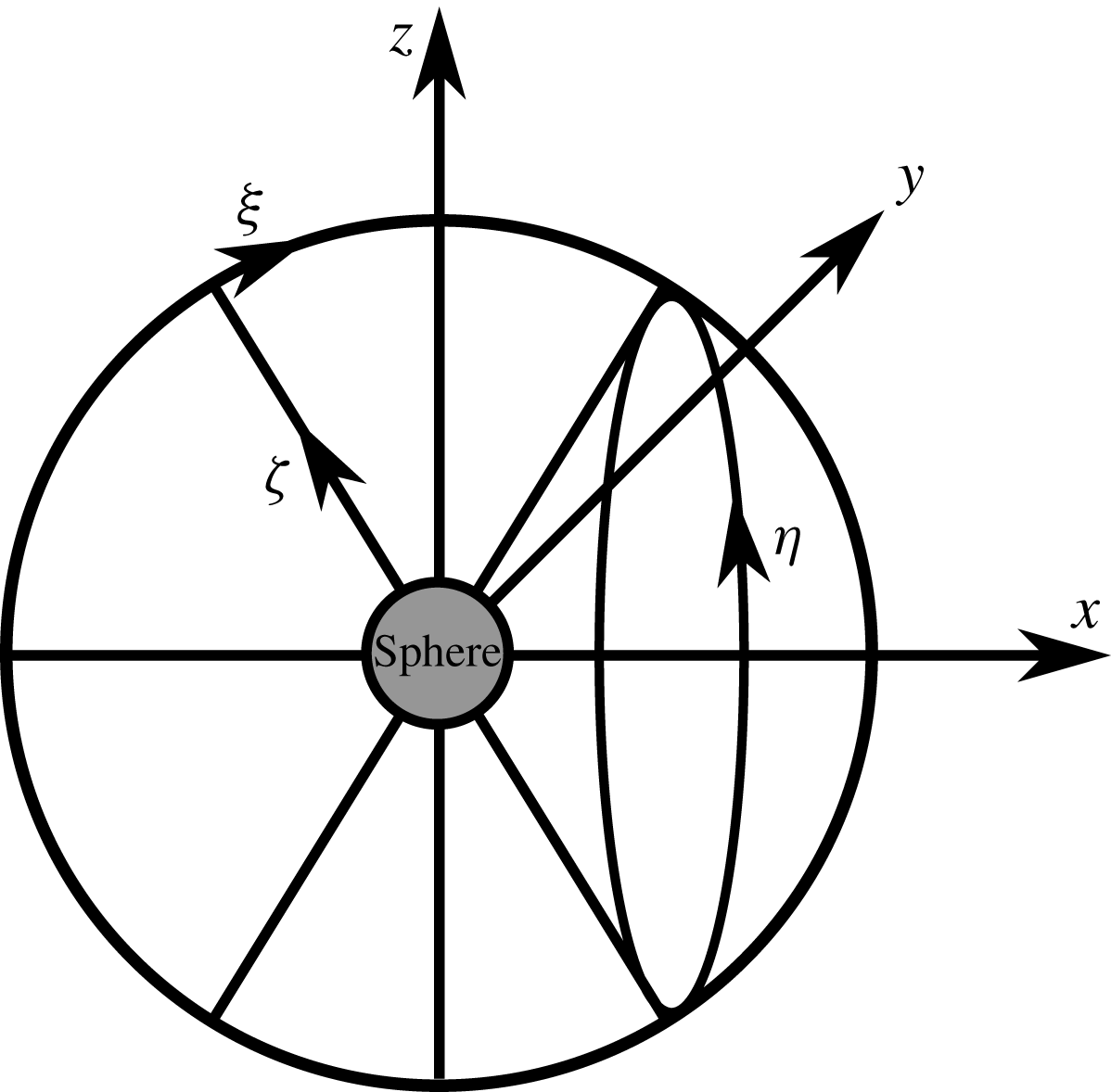
Figure 1. Coordinate system:
 $x$
,
$x$
,
 $y$
and
$y$
and
 $z$
are Cartesian coordinates;
$z$
are Cartesian coordinates;
 $\unicode[STIX]{x1D709}$
,
$\unicode[STIX]{x1D709}$
,
 $\unicode[STIX]{x1D702}$
and
$\unicode[STIX]{x1D702}$
and
 $\unicode[STIX]{x1D701}$
are curvilinear coordinates.
$\unicode[STIX]{x1D701}$
are curvilinear coordinates.
Figure 2. Computational grid: (a) close-up view; (b) far view.
2.4 Boundary conditions and computational conditions
At the boundaries in the
 $\unicode[STIX]{x1D709}$
and
$\unicode[STIX]{x1D709}$
and
 $\unicode[STIX]{x1D702}$
directions, the periodic boundary conditions are imposed on the six overlapped grid points. The boundary condition at the surface of the sphere is adiabatic; also, the velocity on the surface is given as follows to simulate a rotating sphere:
$\unicode[STIX]{x1D702}$
directions, the periodic boundary conditions are imposed on the six overlapped grid points. The boundary condition at the surface of the sphere is adiabatic; also, the velocity on the surface is given as follows to simulate a rotating sphere:
 $$\begin{eqnarray}\displaystyle \left.\begin{array}{@{}c@{}}\displaystyle u_{surf}=\unicode[STIX]{x1D6FA}^{\ast }u_{\infty }\frac{2z}{d},\\ \displaystyle v_{surf}=0,\\ \displaystyle w_{surf}=-\unicode[STIX]{x1D6FA}^{\ast }u_{\infty }\frac{2x}{d},\end{array}\right\} & & \displaystyle\end{eqnarray}$$
where
 $u_{surf}$
,
$u_{surf}$
,
 $v_{surf}$
and
$v_{surf}$
and
 $w_{surf}$
are the
$w_{surf}$
are the
 $x$
,
$x$
,
 $y$
and
$y$
and
 $z$
components of surface velocity, respectively, and
$z$
components of surface velocity, respectively, and
 $x$
and
$x$
and
 $z$
are the position vectors of the
$z$
are the position vectors of the
 $x$
and
$x$
and
 $z$
components. In this study, the axis of rotation is the
$z$
components. In this study, the axis of rotation is the
 $y$
direction. Also, the position and velocity coordinates in polar coordinates along the equator of the sphere are defined in the
$y$
direction. Also, the position and velocity coordinates in polar coordinates along the equator of the sphere are defined in the
 $x$
–
$x$
–
 $z$
plane at
$z$
plane at
 $y=0$
as shown in figure 3 and the flow properties are investigated there. Here,
$y=0$
as shown in figure 3 and the flow properties are investigated there. Here,
 $\unicode[STIX]{x1D703}$
and
$\unicode[STIX]{x1D703}$
and
 $U_{\unicode[STIX]{x1D703}}$
denote the angle from the
$U_{\unicode[STIX]{x1D703}}$
denote the angle from the
 $x$
axis of upstream and the velocity along the equator of the sphere, respectively.
$x$
axis of upstream and the velocity along the equator of the sphere, respectively.

Figure 3. Velocity and position coordinates along the equator of the sphere.
Analysis conditions that are simulated in this study are shown in table 1. In this study, the free-stream Re based on the quantities at the far field and the diameter of the sphere is set between 100 and 300, the free-stream
 $M$
is set between 0.2 and 2.0, and
$M$
is set between 0.2 and 2.0, and
 $\unicode[STIX]{x1D6FA}^{\ast }$
defined by the ratio of the free-stream velocity and the surface velocity above the equator is set between 0.0 and 1.0.
$\unicode[STIX]{x1D6FA}^{\ast }$
defined by the ratio of the free-stream velocity and the surface velocity above the equator is set between 0.0 and 1.0.
Table 1. Analytical conditions.
3 Far-field structure
Under incompressible flows for
 $Re\leqslant 300$
, wake structures are classified into four types (Giacobello et al.
Reference Giacobello, Ooi and Balachandar2009), namely the steady wake, the steady double-threaded wake, the hairpin wake and the one-sided
$Re\leqslant 300$
, wake structures are classified into four types (Giacobello et al.
Reference Giacobello, Ooi and Balachandar2009), namely the steady wake, the steady double-threaded wake, the hairpin wake and the one-sided
 $\unicode[STIX]{x03A9}$
-shaped wake. The flow patterns are changed along with Re and
$\unicode[STIX]{x03A9}$
-shaped wake. The flow patterns are changed along with Re and
 $\unicode[STIX]{x1D6FA}^{\ast }$
. For low-Re and low-
$\unicode[STIX]{x1D6FA}^{\ast }$
. For low-Re and low-
 $\unicode[STIX]{x1D6FA}^{\ast }$
conditions, the flow pattern is the steady wake (e.g.
$\unicode[STIX]{x1D6FA}^{\ast }$
conditions, the flow pattern is the steady wake (e.g.
 $Re=100$
and
$Re=100$
and
 $\unicode[STIX]{x1D6FA}^{\ast }=0.0$
). As Re or
$\unicode[STIX]{x1D6FA}^{\ast }=0.0$
). As Re or
 $\unicode[STIX]{x1D6FA}^{\ast }$
increases, the flow pattern transitions to the steady double-threaded wake (e.g.
$\unicode[STIX]{x1D6FA}^{\ast }$
increases, the flow pattern transitions to the steady double-threaded wake (e.g.
 $Re=100$
and
$Re=100$
and
 $\unicode[STIX]{x1D6FA}^{\ast }=0.3$
). In this flow pattern, two streamwise vortices are generated around the rotation axis of the sphere. For
$\unicode[STIX]{x1D6FA}^{\ast }=0.3$
). In this flow pattern, two streamwise vortices are generated around the rotation axis of the sphere. For
 $Re\geqslant 250$
, the hairpin wake appears. In this flow pattern, the hairpin vortices are periodically released from the recirculation region behind the sphere (e.g.
$Re\geqslant 250$
, the hairpin wake appears. In this flow pattern, the hairpin vortices are periodically released from the recirculation region behind the sphere (e.g.
 $Re=250$
and
$Re=250$
and
 $\unicode[STIX]{x1D6FA}^{\ast }=0.3$
, and
$\unicode[STIX]{x1D6FA}^{\ast }=0.3$
, and
 $Re=300$
and
$Re=300$
and
 $\unicode[STIX]{x1D6FA}^{\ast }=0.3$
). As
$\unicode[STIX]{x1D6FA}^{\ast }=0.3$
). As
 $\unicode[STIX]{x1D6FA}^{\ast }$
further increases, vortex shedding is reduced, and the flow pattern transitions back to the steady double-threaded wake (e.g.
$\unicode[STIX]{x1D6FA}^{\ast }$
further increases, vortex shedding is reduced, and the flow pattern transitions back to the steady double-threaded wake (e.g.
 $Re=300$
and
$Re=300$
and
 $\unicode[STIX]{x1D6FA}^{\ast }=0.6$
). For
$\unicode[STIX]{x1D6FA}^{\ast }=0.6$
). For
 $Re=300$
and
$Re=300$
and
 $\unicode[STIX]{x1D6FA}^{\ast }=0.8$
and 1.0, the flow pattern transitions to the one-sided
$\unicode[STIX]{x1D6FA}^{\ast }=0.8$
and 1.0, the flow pattern transitions to the one-sided
 $\unicode[STIX]{x03A9}$
-shaped wake. In this flow pattern,
$\unicode[STIX]{x03A9}$
-shaped wake. In this flow pattern,
 $\unicode[STIX]{x03A9}$
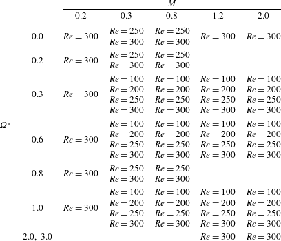
-shaped vortices are generated in the downstream side of the sphere. Figures 4–7 visualize wake structures according to the isosurface of the second invariant value of a velocity gradient tensor (
$\unicode[STIX]{x03A9}$
-shaped vortices are generated in the downstream side of the sphere. Figures 4–7 visualize wake structures according to the isosurface of the second invariant value of a velocity gradient tensor (
 $Q$
-criterion). Here, the
$Q$
-criterion). Here, the
 $Q$
-criterion is calculated by the definition of incompressible flows for visualization except for the shock-wave region, and it is normalized by the free-stream velocity. The
$Q$
-criterion is calculated by the definition of incompressible flows for visualization except for the shock-wave region, and it is normalized by the free-stream velocity. The
 $Q$
-criterion threshold is set at
$Q$
-criterion threshold is set at
 $Q/u^{2}=5.0\times 10^{4}$
. For these figures, the wake structure is influenced not only by Re and
$Q/u^{2}=5.0\times 10^{4}$
. For these figures, the wake structure is influenced not only by Re and
 $\unicode[STIX]{x1D6FA}^{\ast }$
, but also by
$\unicode[STIX]{x1D6FA}^{\ast }$
, but also by
 $M$
. Also, a map of flow pattern type is shown in figure 8.
$M$
. Also, a map of flow pattern type is shown in figure 8.
At
 $Re=300$
and
$Re=300$
and
 $M=0.2$
, the type of flow pattern shows a trend similar to that for incompressible flows. In the case of the one-sided
$M=0.2$
, the type of flow pattern shows a trend similar to that for incompressible flows. In the case of the one-sided
 $\unicode[STIX]{x03A9}$
-shaped wake,
$\unicode[STIX]{x03A9}$
-shaped wake,
 $\unicode[STIX]{x03A9}$
-shaped vortices form downstream of the sphere, and their generation position approaches the sphere as
$\unicode[STIX]{x03A9}$
-shaped vortices form downstream of the sphere, and their generation position approaches the sphere as
 $\unicode[STIX]{x1D6FA}^{\ast }$
increases. The flow pattern clearly transitions from low mode to high mode in the order of the steady flow, the steady double-threaded wake, the hairpin wake, the steady double-threaded wake and the one-sided
$\unicode[STIX]{x1D6FA}^{\ast }$
increases. The flow pattern clearly transitions from low mode to high mode in the order of the steady flow, the steady double-threaded wake, the hairpin wake, the steady double-threaded wake and the one-sided
 $\unicode[STIX]{x03A9}$
-shaped wake as Re and
$\unicode[STIX]{x03A9}$
-shaped wake as Re and
 $\unicode[STIX]{x1D6FA}^{\ast }$
increase for each
$\unicode[STIX]{x1D6FA}^{\ast }$
increase for each
 $M$
.
$M$
.
For
 $Re=300$
and
$Re=300$
and
 $M=0.3$
, the type of flow pattern is similar to that of an incompressible flow for
$M=0.3$
, the type of flow pattern is similar to that of an incompressible flow for
 $\unicode[STIX]{x1D6FA}^{\ast }\leqslant 0.6$
. However, the flow pattern does not transition to the one-sided
$\unicode[STIX]{x1D6FA}^{\ast }\leqslant 0.6$
. However, the flow pattern does not transition to the one-sided
 $\unicode[STIX]{x03A9}$
-shaped wake for
$\unicode[STIX]{x03A9}$
-shaped wake for
 $\unicode[STIX]{x1D6FA}^{\ast }\geqslant 0.8$
. This is thought to be caused by the compressibility effect due to rotation. For high-
$\unicode[STIX]{x1D6FA}^{\ast }\geqslant 0.8$
. This is thought to be caused by the compressibility effect due to rotation. For high-
 $\unicode[STIX]{x1D6FA}^{\ast }$
cases, the fluid velocity at the retreating side (
$\unicode[STIX]{x1D6FA}^{\ast }$
cases, the fluid velocity at the retreating side (
 $y<0$
) and the relative velocity between the free stream and the surface of the sphere at the advancing side (
$y<0$
) and the relative velocity between the free stream and the surface of the sphere at the advancing side (
 $y>0$
) are larger than in stationary cases. Hence, the compressibility effect appears in rotating cases, even in low-
$y>0$
) are larger than in stationary cases. Hence, the compressibility effect appears in rotating cases, even in low-
 $M$
flows. Also, for
$M$
flows. Also, for
 $Re=300$
and
$Re=300$
and
 $M=0.8$
, the hairpin wake appears for
$M=0.8$
, the hairpin wake appears for
 $\unicode[STIX]{x1D6FA}^{\ast }\leqslant 0.8$
, and transitions to the steady double-threaded wake for
$\unicode[STIX]{x1D6FA}^{\ast }\leqslant 0.8$
, and transitions to the steady double-threaded wake for
 $\unicode[STIX]{x1D6FA}^{\ast }=1.0$
. From this result, we believe that the transition of the wake structure to the high mode is suppressed by compressibility effects. This trend has already been reported in the study of the flow past a rotating cylinder under compressible low-Re flows (
$\unicode[STIX]{x1D6FA}^{\ast }=1.0$
. From this result, we believe that the transition of the wake structure to the high mode is suppressed by compressibility effects. This trend has already been reported in the study of the flow past a rotating cylinder under compressible low-Re flows (
 $40\leqslant Re\leqslant 200$
,
$40\leqslant Re\leqslant 200$
,
 $0.05\leqslant M\leqslant 0.4$
and
$0.05\leqslant M\leqslant 0.4$
and
 $0\leqslant \unicode[STIX]{x1D6FA}^{\ast }\leqslant 12$
) by Teymourtash & Salimipour (Reference Teymourtash and Salimipour2017).
$0\leqslant \unicode[STIX]{x1D6FA}^{\ast }\leqslant 12$
) by Teymourtash & Salimipour (Reference Teymourtash and Salimipour2017).
For
 $Re=300$
and
$Re=300$
and
 $M=1.2$
and 2.0 in all cases calculated in this study, the steady wake or steady double-threaded wake appears. In other words, no periodic vortex shedding occurs under supersonic conditions despite
$M=1.2$
and 2.0 in all cases calculated in this study, the steady wake or steady double-threaded wake appears. In other words, no periodic vortex shedding occurs under supersonic conditions despite
 $Re=300$
. This trend is similar to that of low-Re and low-
$Re=300$
. This trend is similar to that of low-Re and low-
 $M$
or incompressible flows. It seems that the flow pattern mode is significantly lower than that in the incompressible or subsonic cases due to the strong compressibility effects. Also, the mode of the flow pattern for
$M$
or incompressible flows. It seems that the flow pattern mode is significantly lower than that in the incompressible or subsonic cases due to the strong compressibility effects. Also, the mode of the flow pattern for
 $M=2.0$
is lower than that of
$M=2.0$
is lower than that of
 $M=1.2$
for the same Re. This trend is similar in the case for
$M=1.2$
for the same Re. This trend is similar in the case for
 $Re\leqslant 250$
as shown in figures 5–7.
$Re\leqslant 250$
as shown in figures 5–7.

Figure 4. Isosurfaces of the second invariant value of the velocity gradient tensor (
 $Q/u_{\infty }^{2}=5.0\times 10^{4}$
) at
$Q/u_{\infty }^{2}=5.0\times 10^{4}$
) at
 $Re=300$
.
$Re=300$
.
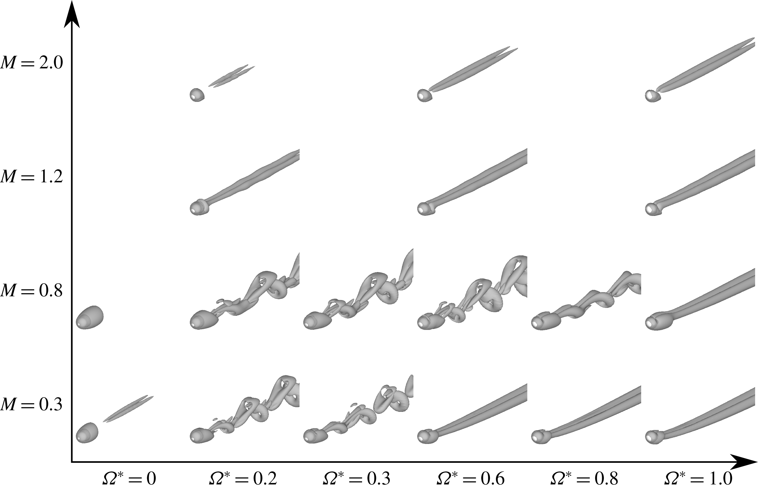
Figure 5. Isosurfaces of the second invariant value of the velocity gradient tensor (
 $Q/u_{\infty }^{2}=5.0\times 10^{4}$
) at
$Q/u_{\infty }^{2}=5.0\times 10^{4}$
) at
 $Re=250$
.
$Re=250$
.
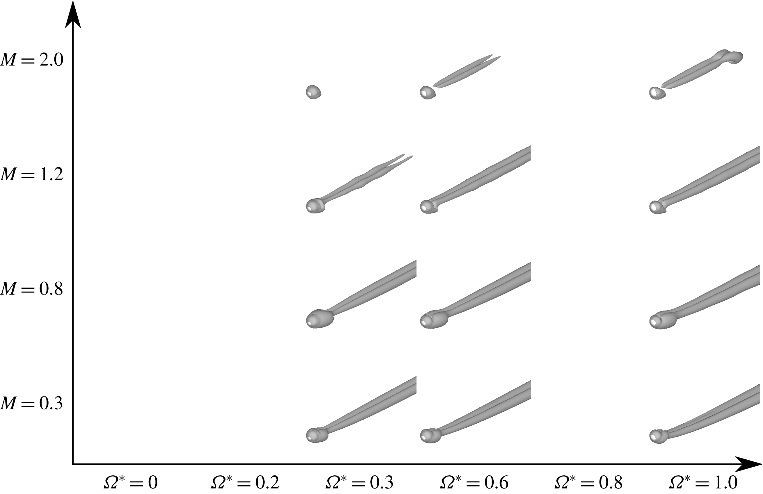
Figure 6. Isosurfaces of the second invariant value of the velocity gradient tensor (
 $Q/u_{\infty }^{2}=5.0\times 10^{4}$
) at
$Q/u_{\infty }^{2}=5.0\times 10^{4}$
) at
 $Re=200$
.
$Re=200$
.
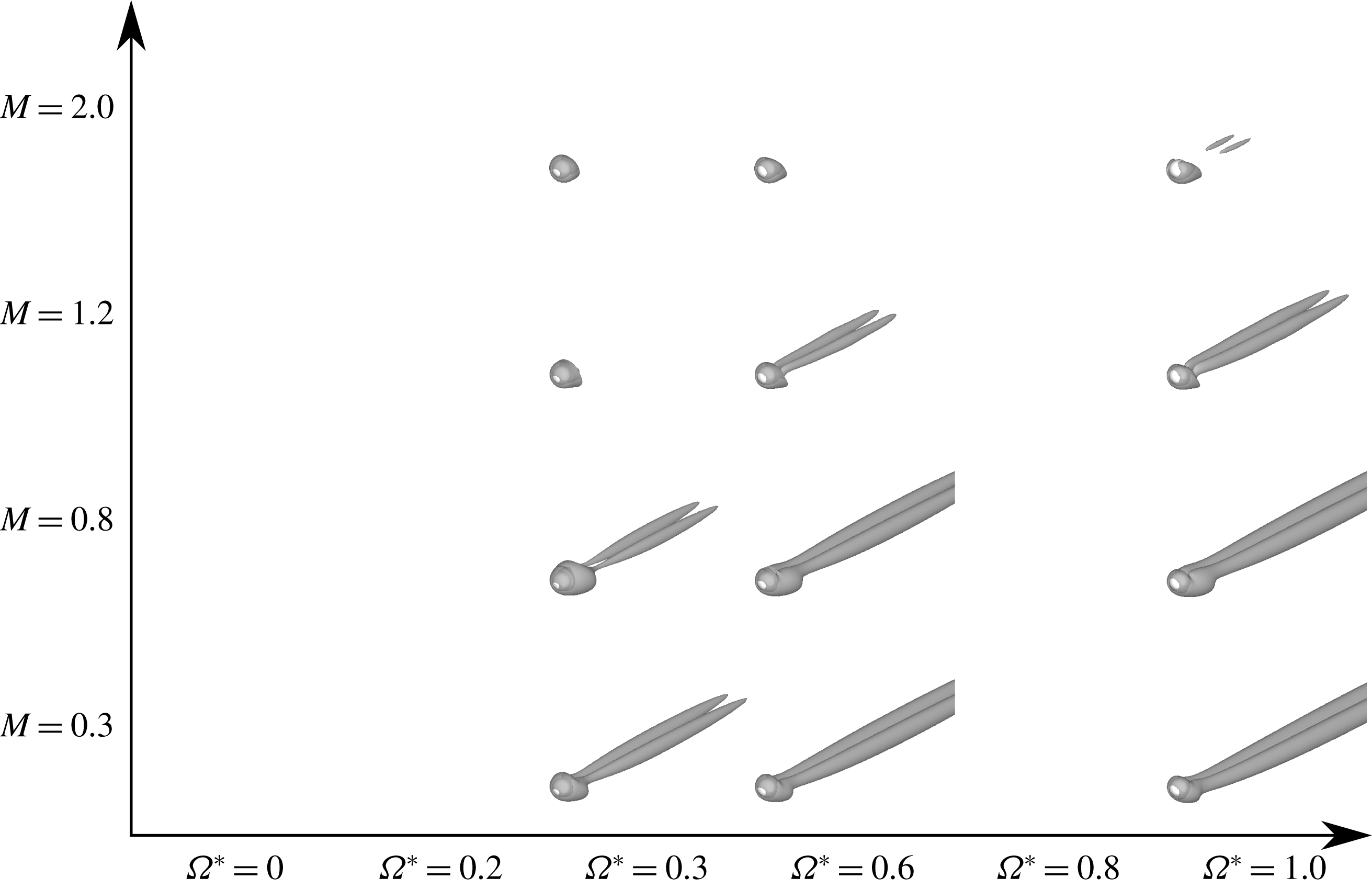
Figure 7. Isosurfaces of the second invariant value of the velocity gradient tensor (
 $Q/u_{\infty }^{2}=5.0\times 10^{4}$
) at
$Q/u_{\infty }^{2}=5.0\times 10^{4}$
) at
 $Re=100$
.
$Re=100$
.
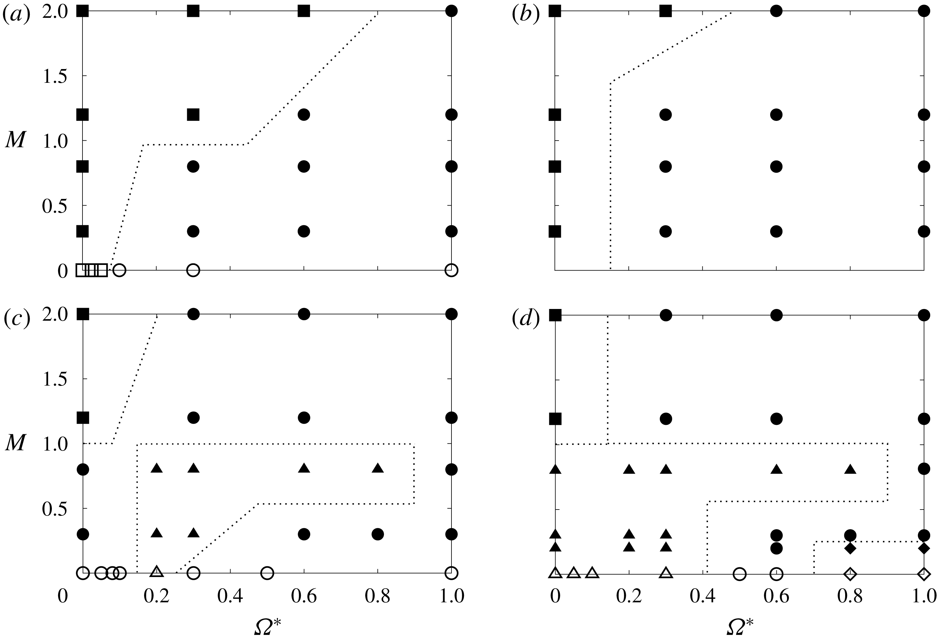
Figure 8. Classification of types of flow pattern: (a)
 $Re=100$
; (b)
$Re=100$
; (b)
 $Re=200$
; (c)
$Re=200$
; (c)
 $Re=250$
; (d)
$Re=250$
; (d)
 $Re=300$
. Results from Giacobello et al. (Reference Giacobello, Ooi and Balachandar2009) (open symbols) and present study (closed symbols). Steady axisymmetric wake (squares); steady double-threaded wake (circles); hairpin wake (triangles); one-sided
$Re=300$
. Results from Giacobello et al. (Reference Giacobello, Ooi and Balachandar2009) (open symbols) and present study (closed symbols). Steady axisymmetric wake (squares); steady double-threaded wake (circles); hairpin wake (triangles); one-sided
 $\unicode[STIX]{x03A9}$
-shaped wake (diamonds).
$\unicode[STIX]{x03A9}$
-shaped wake (diamonds).
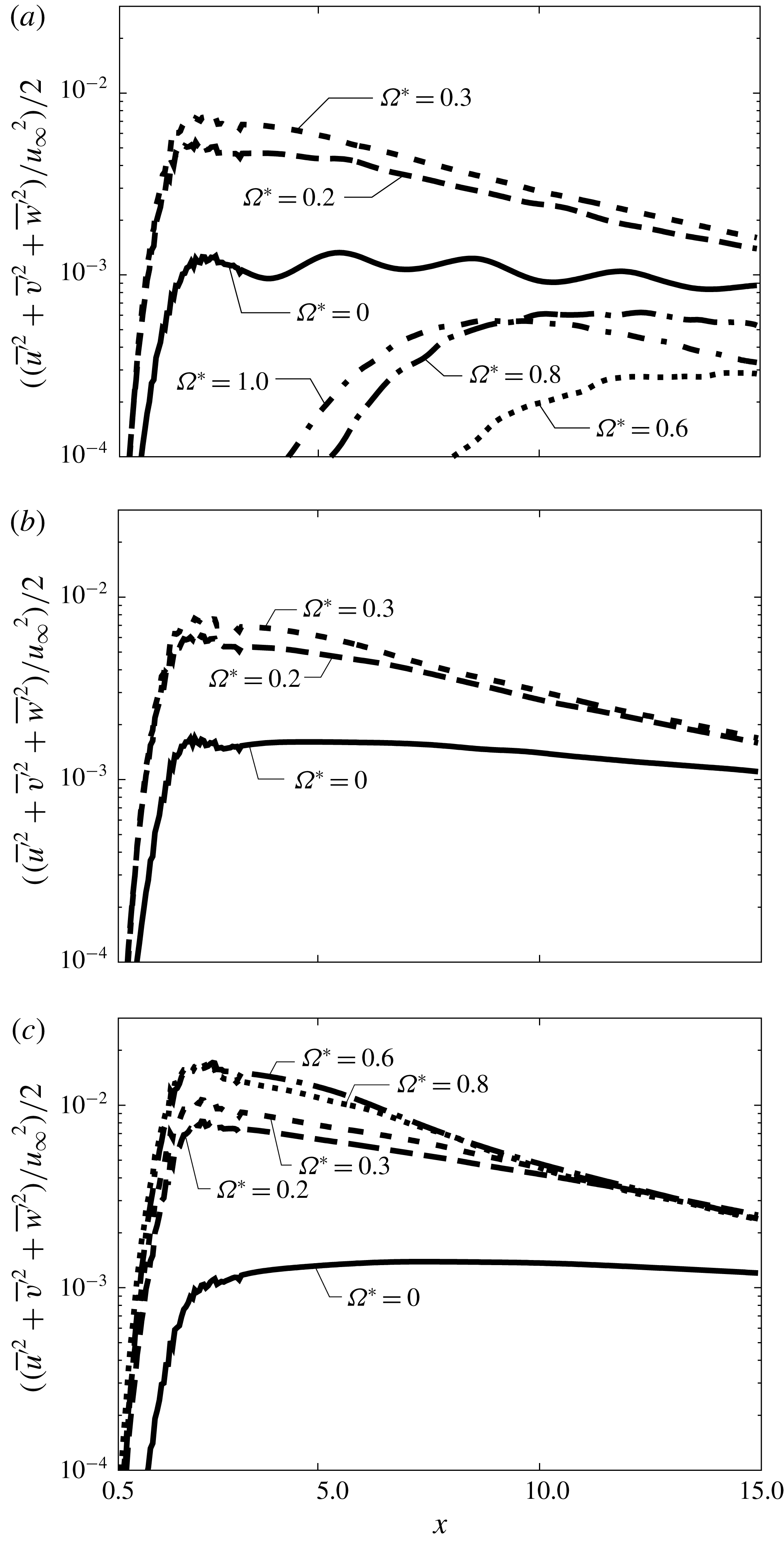
Figure 9. Normalized TKE distribution behind the sphere at
 $Re=300$
: (a)
$Re=300$
: (a)
 $M=0.2$
; (b)
$M=0.2$
; (b)
 $M=0.3$
; (c)
$M=0.3$
; (c)
 $M=0.8$
.
$M=0.8$
.
Figure 9 shows the distribution of volume-averaged turbulent kinetic energy (TKE) normalized by free-stream kinetic energy in the wake. The TKE is calculated in the high-resolution region (
 $0.5\leqslant x\leqslant 15$
and
$0.5\leqslant x\leqslant 15$
and
 $\sqrt{y^{2}+z^{2}}\leqslant 4$
) by the following formula:
$\sqrt{y^{2}+z^{2}}\leqslant 4$
) by the following formula:
 $$\begin{eqnarray}\displaystyle & \displaystyle \overline{\boldsymbol{u}^{\prime }}=\sqrt{\left|\overline{\boldsymbol{u}^{2}}-\bar{\boldsymbol{u}}^{2}\right|}, & \displaystyle\end{eqnarray}$$
 $$\begin{eqnarray}\displaystyle & \displaystyle \text{TKE}=\frac{1}{2}\,\frac{\overline{u}^{\prime 2}+\overline{v}^{\prime 2}+\overline{w}^{\prime 2}}{u_{\infty }^{2}}. & \displaystyle\end{eqnarray}$$
Here, an over-line means time-averaged quantity. It is also volume-averaged for every
 $\text{d}x=0.05$
. In figure 9, the TKE is large in cases that have an unsteady wake. Furthermore, the TKE peak is significantly large in the case of an unsteady wake with rotating cases, even though the wake structure is similar to that of the stationary cases (the hairpin wake). On the other hand, the TKE for the rotating case asymptotically becomes the stationary case in the far field (
$\text{d}x=0.05$
. In figure 9, the TKE is large in cases that have an unsteady wake. Furthermore, the TKE peak is significantly large in the case of an unsteady wake with rotating cases, even though the wake structure is similar to that of the stationary cases (the hairpin wake). On the other hand, the TKE for the rotating case asymptotically becomes the stationary case in the far field (
 $x\approx 15$
). Moreover, the TKE for an
$x\approx 15$
). Moreover, the TKE for an
 $\unicode[STIX]{x03A9}$
-shaped wake (e.g.
$\unicode[STIX]{x03A9}$
-shaped wake (e.g.
 $M=0.2$
and
$M=0.2$
and
 $\unicode[STIX]{x1D6FA}^{\ast }=1.0$
) is relatively small compared with the hairpin wake, even though the wake is unsteady and the TKE peak position occurs farther from the sphere than the hairpin wake. This is due to the difference between the vortex generation processes of the wake in each case. In the case of the hairpin wake, such vortices are generated in the vicinity of the sphere (boundary layer and recirculation region). Therefore, the TKE peak occurs in the vicinity of the sphere. Conversely, for an
$\unicode[STIX]{x1D6FA}^{\ast }=1.0$
) is relatively small compared with the hairpin wake, even though the wake is unsteady and the TKE peak position occurs farther from the sphere than the hairpin wake. This is due to the difference between the vortex generation processes of the wake in each case. In the case of the hairpin wake, such vortices are generated in the vicinity of the sphere (boundary layer and recirculation region). Therefore, the TKE peak occurs in the vicinity of the sphere. Conversely, for an
 $\unicode[STIX]{x03A9}$
-shaped wake, vortices are generated due to the instability of the shear layer. Hence, the TKE peak occurs relatively far downstream compared with the hairpin wake. Furthermore, the TKE peak moves upstream as
$\unicode[STIX]{x03A9}$
-shaped wake, vortices are generated due to the instability of the shear layer. Hence, the TKE peak occurs relatively far downstream compared with the hairpin wake. Furthermore, the TKE peak moves upstream as
 $\unicode[STIX]{x1D6FA}^{\ast }$
increases. In terms of Mach number, for rotating cases of
$\unicode[STIX]{x1D6FA}^{\ast }$
increases. In terms of Mach number, for rotating cases of
 $M=0.8$
, the peak of TKE is larger than
$M=0.8$
, the peak of TKE is larger than
 $M=0.2$
and 0.3. It seems that this is due to the effect of the disturbance caused by the attached shock wave formed at the retreating side, as will be discussed in the next section.
$M=0.2$
and 0.3. It seems that this is due to the effect of the disturbance caused by the attached shock wave formed at the retreating side, as will be discussed in the next section.
Figure 10. Pressure coefficient distributions and streamlines of a time-averaged field at
 $Re=300$
(
$Re=300$
(
 $x$
–
$x$
–
 $z$
plane).
$z$
plane).
4 Near-field structure
Figure 10 shows the pressure coefficient distributions and streamlines in the time-averaged fields obtained over durations longer than 10 vortex-shedding periods in unsteady cases. In stationary cases, the recirculation region in the subsonic and supersonic flows is asymmetric and symmetric, respectively, in the
 $x$
–
$x$
–
 $z$
plane. This asymmetry in the time-averaged field is caused by vortex shedding and the steady non-axisymmetric recirculation region. On the other hand, the symmetric recirculation region appears in supersonic flows because no vortex shedding occurs. Also, the size of the recirculation region expands (shrinks) as
$z$
plane. This asymmetry in the time-averaged field is caused by vortex shedding and the steady non-axisymmetric recirculation region. On the other hand, the symmetric recirculation region appears in supersonic flows because no vortex shedding occurs. Also, the size of the recirculation region expands (shrinks) as
 $M$
increases under subsonic (supersonic) flows. This trend has already been reported by Nagata et al. (Reference Nagata, Nonomura, Takahashi, Mizuno and Fukuda2016). For example, for the stationary sphere at
$M$
increases under subsonic (supersonic) flows. This trend has already been reported by Nagata et al. (Reference Nagata, Nonomura, Takahashi, Mizuno and Fukuda2016). For example, for the stationary sphere at
 $Re=300$
, the recirculation region expands as
$Re=300$
, the recirculation region expands as
 $M$
increases for
$M$
increases for
 $M\leqslant 0.95$
. On the other hand, it shrinks as
$M\leqslant 0.95$
. On the other hand, it shrinks as
 $M$
increases for
$M$
increases for
 $M\geqslant 1.05$
.
$M\geqslant 1.05$
.
In the rotating cases, in subsonic flows, an attached shock wave is formed at the retreating side, and its strength increases along with
 $M$
. As a result, the recirculation region expands as
$M$
. As a result, the recirculation region expands as
 $M$
increases. By the effect of rotation, the flow structure behind the sphere becomes asymmetric under all conditions calculated in this study. For
$M$
increases. By the effect of rotation, the flow structure behind the sphere becomes asymmetric under all conditions calculated in this study. For
 $M=0.3$
, the recirculation region disappears for
$M=0.3$
, the recirculation region disappears for
 $\unicode[STIX]{x1D6FA}^{\ast }\geqslant 0.3$
. However, at
$\unicode[STIX]{x1D6FA}^{\ast }\geqslant 0.3$
. However, at
 $M=0.8$
, this region is retained for
$M=0.8$
, this region is retained for
 $\unicode[STIX]{x1D6FA}^{\ast }\leqslant 0.6$
. This difference is caused by the encouragement of separation due to the disturbance induced by the attached shock wave formed at the retreating side. This effect also appears for
$\unicode[STIX]{x1D6FA}^{\ast }\leqslant 0.6$
. This difference is caused by the encouragement of separation due to the disturbance induced by the attached shock wave formed at the retreating side. This effect also appears for
 $M=1.2$
and
$M=1.2$
and
 $\unicode[STIX]{x1D6FA}^{\ast }=0.3$
. However, for supersonic cases, the recirculation region disappears for
$\unicode[STIX]{x1D6FA}^{\ast }=0.3$
. However, for supersonic cases, the recirculation region disappears for
 $M=1.2$
and
$M=1.2$
and
 $\unicode[STIX]{x1D6FA}^{\ast }\geqslant 0.6$
, and for
$\unicode[STIX]{x1D6FA}^{\ast }\geqslant 0.6$
, and for
 $M=2.0$
and
$M=2.0$
and
 $\unicode[STIX]{x1D6FA}^{\ast }\geqslant 0.3$
, even though the attached shock wave is formed, because the recirculation region in the supersonic flow at the same Re is smaller than that in subsonic cases due to the influence of the expansion wave behind the sphere. It seems that the occurrence of the attached shock has a large impact on the change of the flow properties. Owing to the effect of the attached shock, the flow induced by rotation is decelerated by the shock, and particularly affects the recirculation region. It means that the effect of the rotation is attenuated by the attached shock. For this effect, the transition of the type of flow pattern due to rotation is suppressed by increasing
$\unicode[STIX]{x1D6FA}^{\ast }\geqslant 0.3$
, even though the attached shock wave is formed, because the recirculation region in the supersonic flow at the same Re is smaller than that in subsonic cases due to the influence of the expansion wave behind the sphere. It seems that the occurrence of the attached shock has a large impact on the change of the flow properties. Owing to the effect of the attached shock, the flow induced by rotation is decelerated by the shock, and particularly affects the recirculation region. It means that the effect of the rotation is attenuated by the attached shock. For this effect, the transition of the type of flow pattern due to rotation is suppressed by increasing
 $M$
as discussed in § 3. In addition, as will be discussed in §§ 5.1 and 5.2, the increment of drag and lift coefficients by rotation becomes small as
$M$
as discussed in § 3. In addition, as will be discussed in §§ 5.1 and 5.2, the increment of drag and lift coefficients by rotation becomes small as
 $M$
increases.
$M$
increases.
Figure 11 shows snapshots of the divergences of velocity vectors,
 $\boldsymbol{u}$
, in the time-averaged field. These snapshots are normalized by the free-stream velocity and the diameter of the sphere. For figure 11, the configuration of attached shock waves is significantly influenced by
$\boldsymbol{u}$
, in the time-averaged field. These snapshots are normalized by the free-stream velocity and the diameter of the sphere. For figure 11, the configuration of attached shock waves is significantly influenced by
 $\unicode[STIX]{x1D6FA}^{\ast }$
for each
$\unicode[STIX]{x1D6FA}^{\ast }$
for each
 $M$
. For stationary cases, the attached shock wave appears symmetric under supersonic conditions. For rotating cases, the strength of the attached shock wave formed at the retreating (advancing) side becomes strong (weak) as
$M$
. For stationary cases, the attached shock wave appears symmetric under supersonic conditions. For rotating cases, the strength of the attached shock wave formed at the retreating (advancing) side becomes strong (weak) as
 $\unicode[STIX]{x1D6FA}^{\ast }$
increases. Also, the angle of the attached shock wave formed at the retreating side becomes similar to that under high-
$\unicode[STIX]{x1D6FA}^{\ast }$
increases. Also, the angle of the attached shock wave formed at the retreating side becomes similar to that under high-
 $M$
conditions as
$M$
conditions as
 $\unicode[STIX]{x1D6FA}^{\ast }$
increases. This is due to acceleration and deceleration of fluid on the retreating and advancing sides, respectively. Also, for
$\unicode[STIX]{x1D6FA}^{\ast }$
increases. This is due to acceleration and deceleration of fluid on the retreating and advancing sides, respectively. Also, for
 $M=0.8$
, a normal shock wave is formed at the retreating side and its strength increases along with
$M=0.8$
, a normal shock wave is formed at the retreating side and its strength increases along with
 $\unicode[STIX]{x1D6FA}^{\ast }$
.
$\unicode[STIX]{x1D6FA}^{\ast }$
.
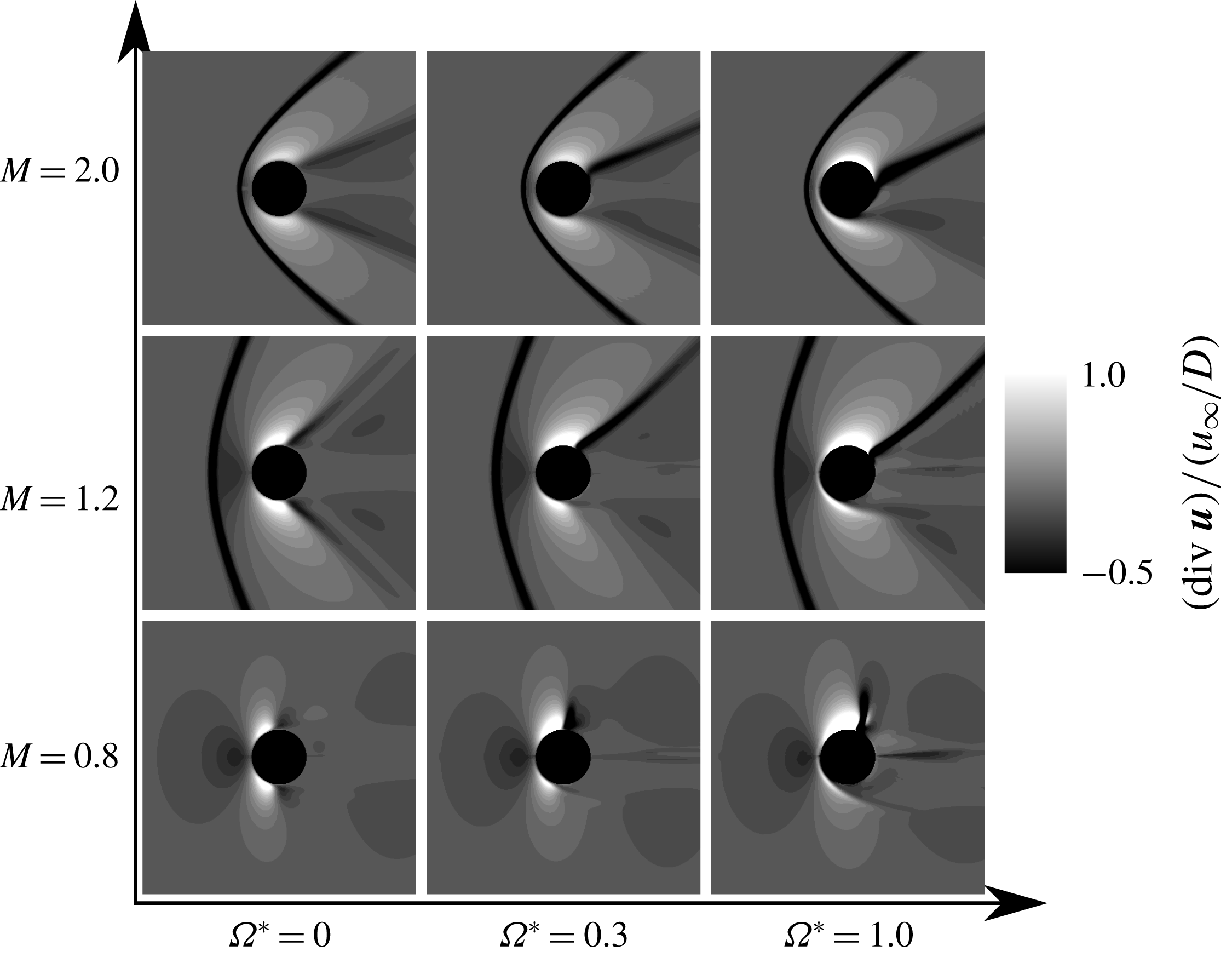
Figure 11. Schlieren-like images over a time-averaged field at
 $Re=300$
(
$Re=300$
(
 $x$
–
$x$
–
 $z$
plane).
$z$
plane).
5 Hydrodynamic force coefficients
5.1 Lift coefficient
Figure 12 shows the relationship between
 $\unicode[STIX]{x1D6FA}^{\ast }$
and
$\unicode[STIX]{x1D6FA}^{\ast }$
and
 $C_{L}$
. In the case of the rotating sphere in incompressible flow, it is well known that the lift force is mainly generated by the pressure difference between the retreating and advancing sides caused by the velocity difference. In figure 12, the results for incompressible flows given by Kurose & Komori (Reference Kurose and Komori1999), Niazmand & Renksizbulut (Reference Niazmand and Renksizbulut2003), Giacobello et al. (Reference Giacobello, Ooi and Balachandar2009) and Dobson et al. (Reference Dobson, Ooi and Poon2014) are shown as grey symbols. From figure 12,
$C_{L}$
. In the case of the rotating sphere in incompressible flow, it is well known that the lift force is mainly generated by the pressure difference between the retreating and advancing sides caused by the velocity difference. In figure 12, the results for incompressible flows given by Kurose & Komori (Reference Kurose and Komori1999), Niazmand & Renksizbulut (Reference Niazmand and Renksizbulut2003), Giacobello et al. (Reference Giacobello, Ooi and Balachandar2009) and Dobson et al. (Reference Dobson, Ooi and Poon2014) are shown as grey symbols. From figure 12,
 $C_{L}$
increases as
$C_{L}$
increases as
 $\unicode[STIX]{x1D6FA}^{\ast }$
increases, and the
$\unicode[STIX]{x1D6FA}^{\ast }$
increases, and the
 $C_{L}$
dependence for
$C_{L}$
dependence for
 $M=0.3$
agrees with the result for the incompressible flows. However, the increment of
$M=0.3$
agrees with the result for the incompressible flows. However, the increment of
 $C_{L}$
due to rotation decreases as
$C_{L}$
due to rotation decreases as
 $M$
increases. This trend is similar even though
$M$
increases. This trend is similar even though
 $Re<300$
, but the increment of
$Re<300$
, but the increment of
 $C_{L}$
becomes larger at low-Re conditions. Those
$C_{L}$
becomes larger at low-Re conditions. Those
 $M$
and Re effects on
$M$
and Re effects on
 $C_{L}$
are similar to the results for a cylinder under compressible flow reported by Teymourtash & Salimipour (Reference Teymourtash and Salimipour2017). In addition, according to the results for incompressible flow at
$C_{L}$
are similar to the results for a cylinder under compressible flow reported by Teymourtash & Salimipour (Reference Teymourtash and Salimipour2017). In addition, according to the results for incompressible flow at
 $1.0<\unicode[STIX]{x1D6FA}^{\ast }\leqslant 3.0$
by Dobson et al. (Reference Dobson, Ooi and Poon2014),
$1.0<\unicode[STIX]{x1D6FA}^{\ast }\leqslant 3.0$
by Dobson et al. (Reference Dobson, Ooi and Poon2014),
 $C_{L}$
due to rotation saturates at approximately
$C_{L}$
due to rotation saturates at approximately
 $\unicode[STIX]{x1D6FA}^{\ast }=1.0$
and
$\unicode[STIX]{x1D6FA}^{\ast }=1.0$
and
 $C_{L}=0.6$
. However, in the case of the supersonic conditions,
$C_{L}=0.6$
. However, in the case of the supersonic conditions,
 $C_{L}$
continuously increases for
$C_{L}$
continuously increases for
 $1.0<\unicode[STIX]{x1D6FA}^{\ast }\leqslant 3.0$
. It is considered that the upper bound of
$1.0<\unicode[STIX]{x1D6FA}^{\ast }\leqslant 3.0$
. It is considered that the upper bound of
 $C_{L}$
due to rotation and its critical
$C_{L}$
due to rotation and its critical
 $\unicode[STIX]{x1D6FA}^{\ast }$
are influenced by
$\unicode[STIX]{x1D6FA}^{\ast }$
are influenced by
 $M$
.
$M$
.
The normalized lift coefficient
 $C_{L}/C_{L_{incomp}}$
is shown in figure 13, where
$C_{L}/C_{L_{incomp}}$
is shown in figure 13, where
 $C_{L}$
monotonically decreases as
$C_{L}$
monotonically decreases as
 $M$
increases. The
$M$
increases. The
 $\unicode[STIX]{x1D6FA}^{\ast }$
dependence on
$\unicode[STIX]{x1D6FA}^{\ast }$
dependence on
 $C_{L}/C_{L_{incomp}}$
is changed around
$C_{L}/C_{L_{incomp}}$
is changed around
 $M=0.8$
. Under rotating highly subsonic conditions,
$M=0.8$
. Under rotating highly subsonic conditions,
 $M\geqslant 0.8$
and
$M\geqslant 0.8$
and
 $\unicode[STIX]{x1D6FA}^{\ast }\geqslant 0.2$
, the normal shock wave is formed on the retreating side because the flow velocity surpasses the sonic speed in a limited region on the retreating side due to rotation. Hence, the lift force caused by the rotation becomes smaller than in incompressible cases because of the decrease of the velocity difference (pressure difference) between the retreating and advancing sides.
$\unicode[STIX]{x1D6FA}^{\ast }\geqslant 0.2$
, the normal shock wave is formed on the retreating side because the flow velocity surpasses the sonic speed in a limited region on the retreating side due to rotation. Hence, the lift force caused by the rotation becomes smaller than in incompressible cases because of the decrease of the velocity difference (pressure difference) between the retreating and advancing sides.
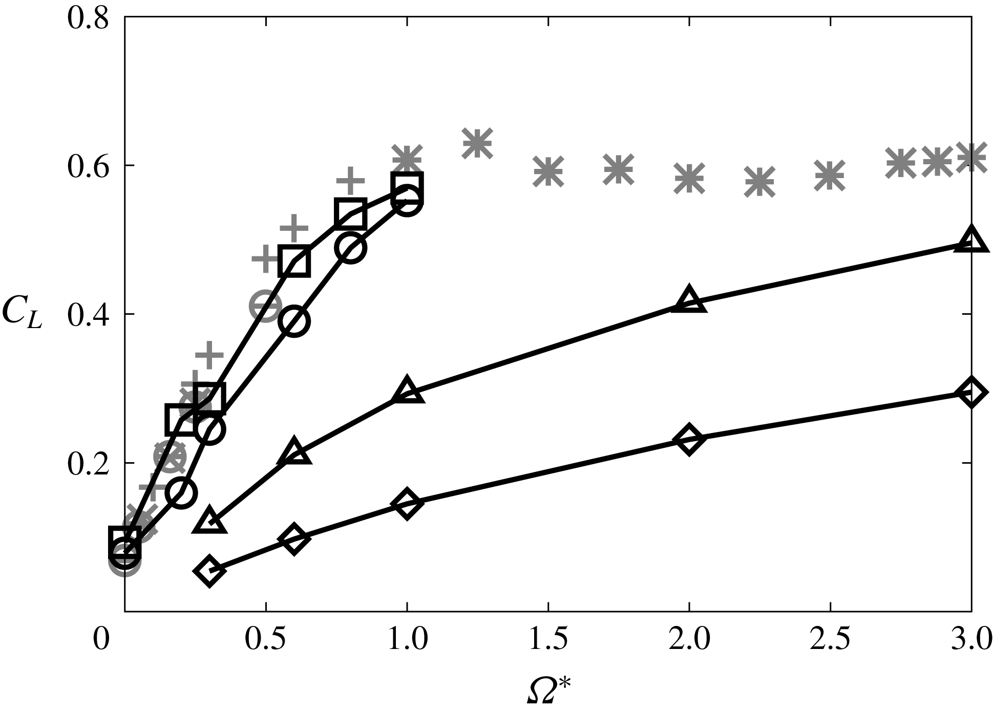
Figure 12. Time-averaged
 $C_{L}$
at
$C_{L}$
at
 $Re=300$
as a function of
$Re=300$
as a function of
 $\unicode[STIX]{x1D6FA}^{\ast }$
. Results for incompressible flows:
$\unicode[STIX]{x1D6FA}^{\ast }$
. Results for incompressible flows:
 $M=0.3$
;
$M=0.3$
;  $M=0.8$
;
$M=0.8$
;  $M=1.2$
;
$M=1.2$
;  $M=2.0$
.
$M=2.0$
.
Figure 13. Dependence of
 $M$
on the increment of
$M$
on the increment of
 $C_{LY}$
at
$C_{LY}$
at
 $Re=300$
:
$Re=300$
:
 $\unicode[STIX]{x1D6FA}^{\ast }=0.3$
;
$\unicode[STIX]{x1D6FA}^{\ast }=0.3$
;  $\unicode[STIX]{x1D6FA}^{\ast }=0.6$
;
$\unicode[STIX]{x1D6FA}^{\ast }=0.6$
;  $\unicode[STIX]{x1D6FA}^{\ast }=1.0$
.
$\unicode[STIX]{x1D6FA}^{\ast }=1.0$
.
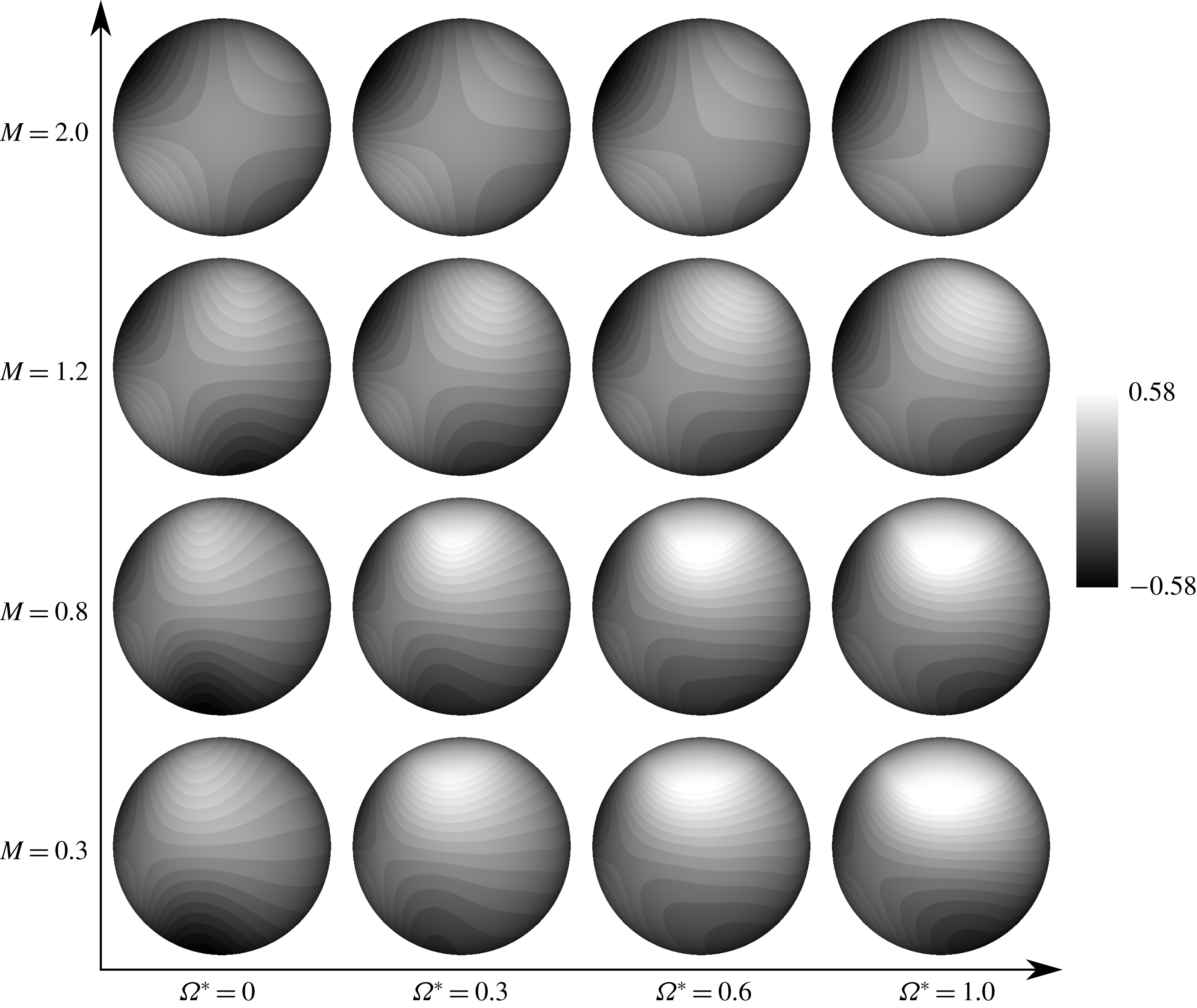
Figure 14. Distribution of the hydrodynamic stress coefficient in the lift force direction for a time-averaged field at
 $Re=300$
(view from
$Re=300$
(view from
 $-y$
).
$-y$
).
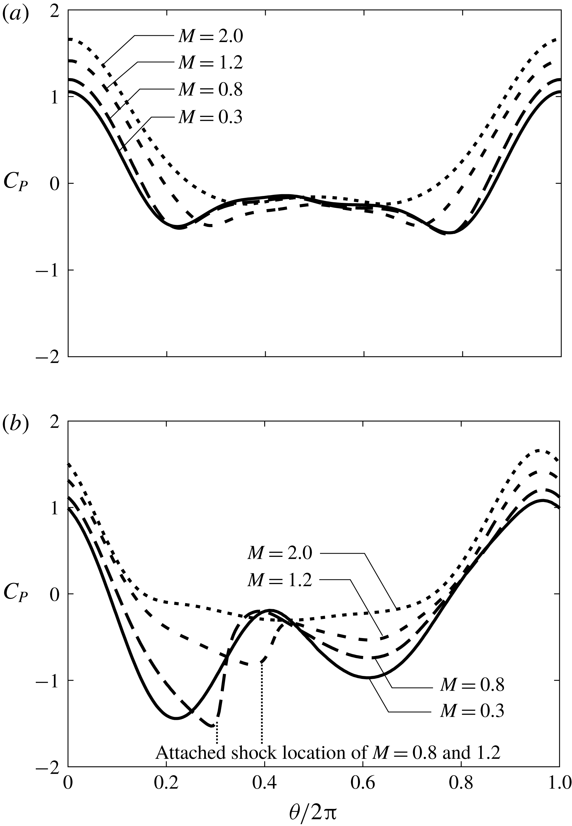
Figure 15. Pressure coefficient distribution at the surface of the sphere above the equator at
 $Re=300$
: (a)
$Re=300$
: (a)
 $\unicode[STIX]{x1D6FA}^{\ast }=0.0$
; (b)
$\unicode[STIX]{x1D6FA}^{\ast }=0.0$
; (b)
 $\unicode[STIX]{x1D6FA}^{\ast }=1.0$
.
$\unicode[STIX]{x1D6FA}^{\ast }=1.0$
.
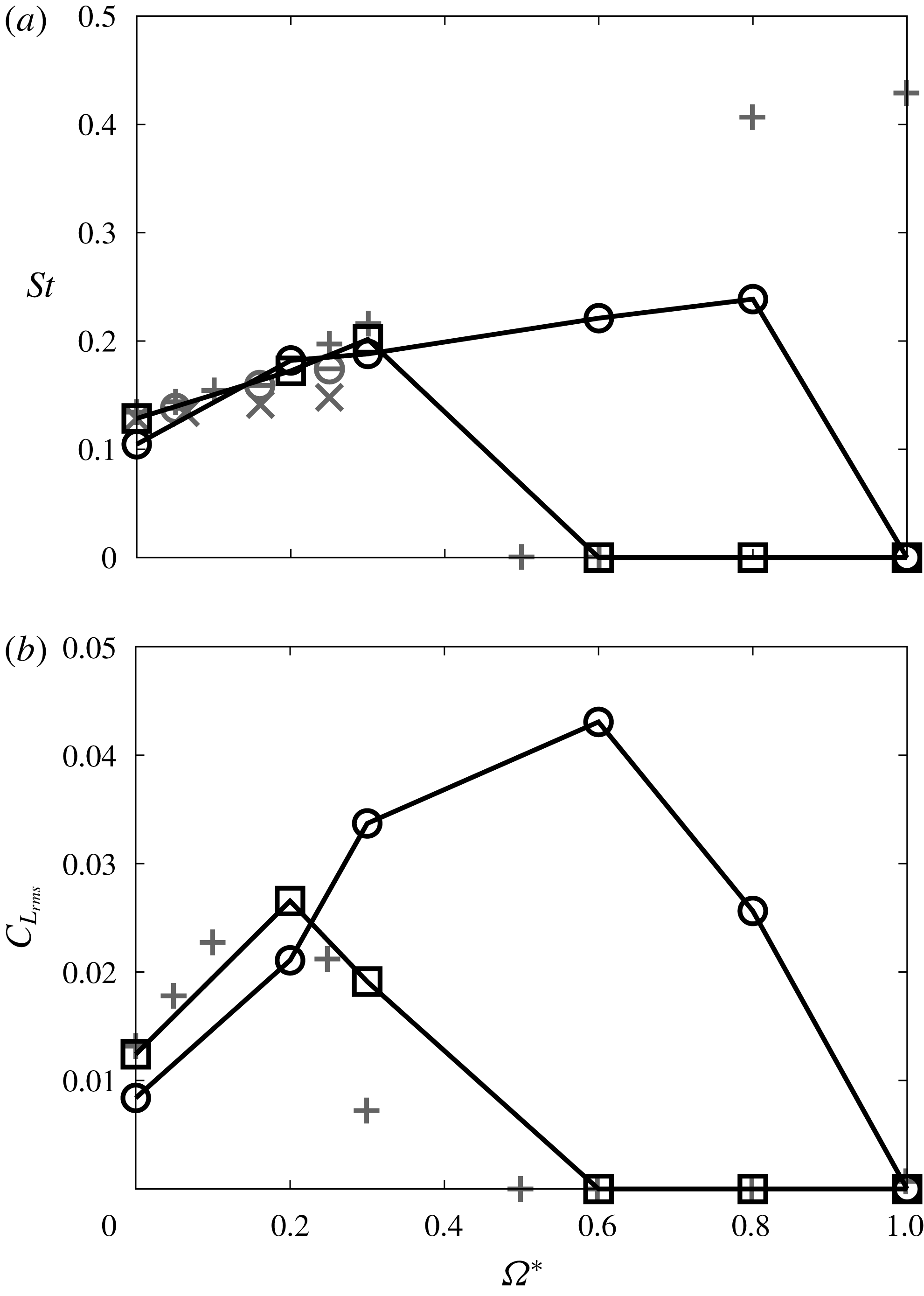
Figure 16. Comparison of the time variation of lift coefficients with the incompressible flow results at
 $Re=300$
: (
$Re=300$
: (
 $a$
) Strouhal number; (
$a$
) Strouhal number; (
 $b$
) r.m.s. amplitude. Incompressible:
$b$
) r.m.s. amplitude. Incompressible:
 $M=0.3$
;
$M=0.3$
;  $M=0.8$
.
$M=0.8$
. Figure 14 shows the hydrodynamic stress distribution for the lift force direction in the time-averaged field. For
 $M=0.3$
, the lift force is generated over a wide area of the retreating side, and its area shrinks and the position moves to the downstream side as
$M=0.3$
, the lift force is generated over a wide area of the retreating side, and its area shrinks and the position moves to the downstream side as
 $M$
increases. On the other hand, the distribution of the hydrodynamic stress in the lift force direction hardly changes with rotation at
$M$
increases. On the other hand, the distribution of the hydrodynamic stress in the lift force direction hardly changes with rotation at
 $M=2.0$
. The lift force by rotation is mainly due to the pressure component. To quantify and analyse the lift force distribution, the pressure coefficient distributions on the surface of the sphere above the equator for
$M=2.0$
. The lift force by rotation is mainly due to the pressure component. To quantify and analyse the lift force distribution, the pressure coefficient distributions on the surface of the sphere above the equator for
 $\unicode[STIX]{x1D6FA}^{\ast }=0.0$
and 1.0 in each
$\unicode[STIX]{x1D6FA}^{\ast }=0.0$
and 1.0 in each
 $M$
are shown in figure 15. For this figure, the pressure coefficient distribution is drastically changed by rotation, and its variation along the equator becomes small as
$M$
are shown in figure 15. For this figure, the pressure coefficient distribution is drastically changed by rotation, and its variation along the equator becomes small as
 $M$
increases. In the case of
$M$
increases. In the case of
 $M=0.3$
, a peak of negative pressure at around
$M=0.3$
, a peak of negative pressure at around
 $\unicode[STIX]{x1D703}/\unicode[STIX]{x03C0}=0.25$
becomes large as
$\unicode[STIX]{x1D703}/\unicode[STIX]{x03C0}=0.25$
becomes large as
 $\unicode[STIX]{x1D6FA}^{\ast }$
increases. On the other hand, the negative pressure region around
$\unicode[STIX]{x1D6FA}^{\ast }$
increases. On the other hand, the negative pressure region around
 $\unicode[STIX]{x1D703}/\unicode[STIX]{x03C0}=0.75$
moves towards
$\unicode[STIX]{x1D703}/\unicode[STIX]{x03C0}=0.75$
moves towards
 $\unicode[STIX]{x1D703}/\unicode[STIX]{x03C0}=0.6$
as
$\unicode[STIX]{x1D703}/\unicode[STIX]{x03C0}=0.6$
as
 $\unicode[STIX]{x1D6FA}^{\ast }$
increases. Also, a stagnation point moves slightly towards the advancing side, and the pressure coefficient around
$\unicode[STIX]{x1D6FA}^{\ast }$
increases. Also, a stagnation point moves slightly towards the advancing side, and the pressure coefficient around
 $\unicode[STIX]{x1D703}/\unicode[STIX]{x03C0}=0.75$
–1.0 increases as
$\unicode[STIX]{x1D703}/\unicode[STIX]{x03C0}=0.75$
–1.0 increases as
 $\unicode[STIX]{x1D6FA}^{\ast }$
increases. Thus, the lift force increases due to rotation. For
$\unicode[STIX]{x1D6FA}^{\ast }$
increases. Thus, the lift force increases due to rotation. For
 $M=0.8$
and 1.2, the negative pressure region around
$M=0.8$
and 1.2, the negative pressure region around
 $\unicode[STIX]{x1D703}/\unicode[STIX]{x03C0}=0.3$
moves to the downstream side and sharply recovers compared with the
$\unicode[STIX]{x1D703}/\unicode[STIX]{x03C0}=0.3$
moves to the downstream side and sharply recovers compared with the
 $M=0.3$
case due to the influence of the attached shock wave. Also, the negative pressure becomes small as
$M=0.3$
case due to the influence of the attached shock wave. Also, the negative pressure becomes small as
 $M$
increases. In addition, there is no large impact of rotation on the pressure coefficient distribution at
$M$
increases. In addition, there is no large impact of rotation on the pressure coefficient distribution at
 $M=2.0$
. For this effect, the increased amount of the lift coefficient due to rotation decreases under high-
$M=2.0$
. For this effect, the increased amount of the lift coefficient due to rotation decreases under high-
 $M$
conditions.
$M$
conditions.
Kajishima (Reference Kajishima2004) suggested that a particle cluster is formed by the influence of the wake vortices released from particles. On the other hand, the lift force due to particle rotation suppresses the formation of particle clusters. The particle rotation is caused by the relative velocity difference inside and outside of the particle cluster at the cluster’s edge. However, for the DNS result, the lift force caused by the particle rotation in the compressible flow is smaller than that of the incompressible flows. Therefore, the particle cluster breakdown due to the particle rotation is suppressed by the compressibility effects. On the other hand, the wake vortices released from the particle are reduced as
 $M$
increases, so that the formation of a particle cluster is suppressed by the compressibility effects. Hence, the effect of the compressibility on the lift force due to the particle rotation and wake vortices released from particles are opposite regarding the formation of a particle cluster. The particle distribution is possibly influenced by the relative
$M$
increases, so that the formation of a particle cluster is suppressed by the compressibility effects. Hence, the effect of the compressibility on the lift force due to the particle rotation and wake vortices released from particles are opposite regarding the formation of a particle cluster. The particle distribution is possibly influenced by the relative
 $M$
of the particles and fluid, but flow simulation using particle-resolved DNS is necessary to discuss the compressibility effect on a particle cluster.
$M$
of the particles and fluid, but flow simulation using particle-resolved DNS is necessary to discuss the compressibility effect on a particle cluster.
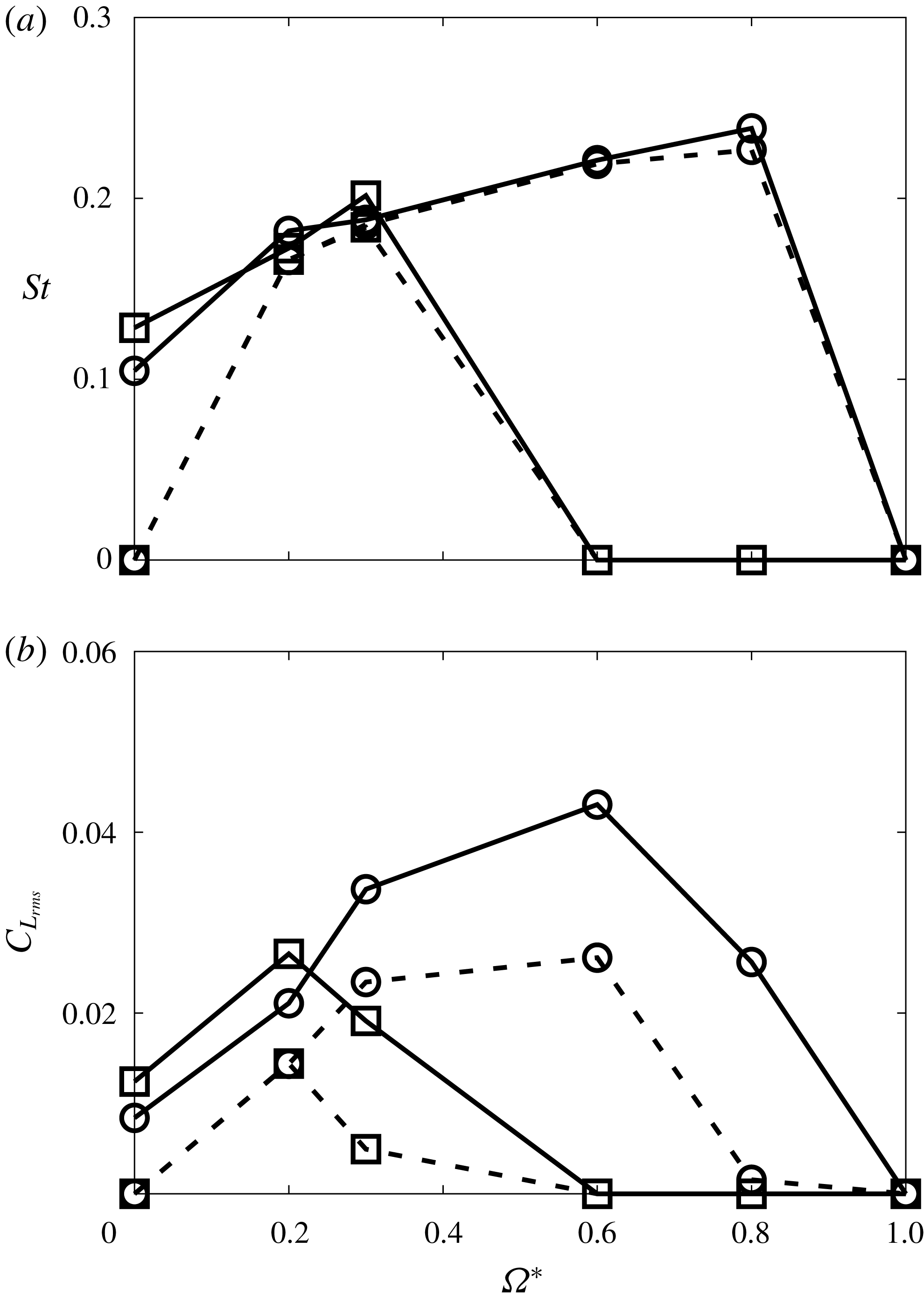
Figure 17. The Re dependence of the time variation of
 $C_{L}$
with (
$C_{L}$
with (
 $a$
) Strouhal number and (
$a$
) Strouhal number and (
 $b$
) r.m.s. amplitude:
$b$
) r.m.s. amplitude:
 $M=0.3$
;
$M=0.3$
;  $M=0.8$
; dotted line,
$M=0.8$
; dotted line,
 $Re=250$
; solid line,
$Re=250$
; solid line,
 $Re=300$
.
$Re=300$
. Figures 16(
 $a$
) and 17(
$a$
) and 17(
 $b$
) show the Strouhal number, St, and the root-mean-square (r.m.s.) amplitude of
$b$
) show the Strouhal number, St, and the root-mean-square (r.m.s.) amplitude of
 $C_{L}$
at
$C_{L}$
at
 $Re=300$
, respectively. The results under the compressible flows are compared with the results under the incompressible flows by Kurose & Komori (Reference Kurose and Komori1999), Niazmand & Renksizbulut (Reference Niazmand and Renksizbulut2003) and Giacobello et al. (Reference Giacobello, Ooi and Balachandar2009). For figure 16(
$Re=300$
, respectively. The results under the compressible flows are compared with the results under the incompressible flows by Kurose & Komori (Reference Kurose and Komori1999), Niazmand & Renksizbulut (Reference Niazmand and Renksizbulut2003) and Giacobello et al. (Reference Giacobello, Ooi and Balachandar2009). For figure 16(
 $a$
), the Strouhal number under incompressible flows and
$a$
), the Strouhal number under incompressible flows and
 $M\leqslant 0.3$
increases with
$M\leqslant 0.3$
increases with
 $\unicode[STIX]{x1D6FA}^{\ast }$
for
$\unicode[STIX]{x1D6FA}^{\ast }$
for
 $\unicode[STIX]{x1D6FA}^{\ast }\leqslant 0.3$
. As
$\unicode[STIX]{x1D6FA}^{\ast }\leqslant 0.3$
. As
 $\unicode[STIX]{x1D6FA}^{\ast }$
further increases, the Strouhal number becomes temporarily zero because the flow regime becomes the steady double-threaded wake (i.e. steady). For
$\unicode[STIX]{x1D6FA}^{\ast }$
further increases, the Strouhal number becomes temporarily zero because the flow regime becomes the steady double-threaded wake (i.e. steady). For
 $\unicode[STIX]{x1D6FA}^{\ast }\geqslant 0.8$
, the flow pattern becomes the one-sided
$\unicode[STIX]{x1D6FA}^{\ast }\geqslant 0.8$
, the flow pattern becomes the one-sided
 $\unicode[STIX]{x03A9}$
-shaped wake in incompressible flow and
$\unicode[STIX]{x03A9}$
-shaped wake in incompressible flow and
 $M=0.2$
. In this flow pattern, vortex shedding occurs more frequently than in the case of the hairpin wake. The Strouhal number ranges from double to four times that for the hairpin wake. On the other hand, in compressible flows, a different trend can be seen. In the case of
$M=0.2$
. In this flow pattern, vortex shedding occurs more frequently than in the case of the hairpin wake. The Strouhal number ranges from double to four times that for the hairpin wake. On the other hand, in compressible flows, a different trend can be seen. In the case of
 $M=0.3$
and
$M=0.3$
and
 $\unicode[STIX]{x1D6FA}^{\ast }=0.6$
, the Strouhal number is zero, as in incompressible flows. However, it remains zero even if
$\unicode[STIX]{x1D6FA}^{\ast }=0.6$
, the Strouhal number is zero, as in incompressible flows. However, it remains zero even if
 $\unicode[STIX]{x1D6FA}^{\ast }=0.8$
and 1.0. Also, for
$\unicode[STIX]{x1D6FA}^{\ast }=0.8$
and 1.0. Also, for
 $M=0.8$
, the Strouhal number is not zero at
$M=0.8$
, the Strouhal number is not zero at
 $\unicode[STIX]{x1D6FA}^{\ast }=0.6$
and 0.8. These different trends are caused by differences in the flow pattern due to compressibility effects. For figure 16(
$\unicode[STIX]{x1D6FA}^{\ast }=0.6$
and 0.8. These different trends are caused by differences in the flow pattern due to compressibility effects. For figure 16(
 $b$
), the r.m.s. amplitude of
$b$
), the r.m.s. amplitude of
 $C_{L}$
for
$C_{L}$
for
 $M=0.3$
has a peak at
$M=0.3$
has a peak at
 $\unicode[STIX]{x1D6FA}^{\ast }=0.2$
similar to incompressible flow. On the other hand, for
$\unicode[STIX]{x1D6FA}^{\ast }=0.2$
similar to incompressible flow. On the other hand, for
 $M=0.8$
, the peak r.m.s. amplitude of
$M=0.8$
, the peak r.m.s. amplitude of
 $C_{L}$
appears at
$C_{L}$
appears at
 $\unicode[STIX]{x1D6FA}^{\ast }=0.6$
and its value is approximately 1.5 times that of the incompressible cases.
$\unicode[STIX]{x1D6FA}^{\ast }=0.6$
and its value is approximately 1.5 times that of the incompressible cases.
Figure 17 compares the Strouhal number and r.m.s. of
 $C_{L}$
calculated at
$C_{L}$
calculated at
 $Re=250$
and 300 and
$Re=250$
and 300 and
 $M=0.3$
and 0.8. For figure 17, the Strouhal number is almost the same for each
$M=0.3$
and 0.8. For figure 17, the Strouhal number is almost the same for each
 $M$
except
$M$
except
 $\unicode[STIX]{x1D6FA}^{\ast }=0.0$
. In other words, for the same flow pattern, Re has no effect upon the Strouhal number of the vortex shedding. On the other hand, the r.m.s. amplitude of
$\unicode[STIX]{x1D6FA}^{\ast }=0.0$
. In other words, for the same flow pattern, Re has no effect upon the Strouhal number of the vortex shedding. On the other hand, the r.m.s. amplitude of
 $C_{L}$
becomes small as Re decreases. Thus, the frequency of vortex shedding is barely not affected by Re, but its strength weakens as Re decreases.
$C_{L}$
becomes small as Re decreases. Thus, the frequency of vortex shedding is barely not affected by Re, but its strength weakens as Re decreases.
5.2 Drag coefficient
Figure 18 shows the relationship between
 $\unicode[STIX]{x1D6FA}^{\ast }$
and drag coefficient,
$\unicode[STIX]{x1D6FA}^{\ast }$
and drag coefficient,
 $C_{D}$
, at
$C_{D}$
, at
 $Re=300$
. From figure 18,
$Re=300$
. From figure 18,
 $C_{D}$
at
$C_{D}$
at
 $M=0.3$
shows a very similar trend to previous incompressible studies. The total drag coefficient basically increases as
$M=0.3$
shows a very similar trend to previous incompressible studies. The total drag coefficient basically increases as
 $\unicode[STIX]{x1D6FA}^{\ast }$
increases. Also, this increment of
$\unicode[STIX]{x1D6FA}^{\ast }$
increases. Also, this increment of
 $C_{D}$
with
$C_{D}$
with
 $\unicode[STIX]{x1D6FA}^{\ast }$
becomes small as
$\unicode[STIX]{x1D6FA}^{\ast }$
becomes small as
 $M$
increases. This trend is similar to the result of a cylinder under compressible flow by Teymourtash & Salimipour (Reference Teymourtash and Salimipour2017). Also, at
$M$
increases. This trend is similar to the result of a cylinder under compressible flow by Teymourtash & Salimipour (Reference Teymourtash and Salimipour2017). Also, at
 $M=0.8$
, the increment of the drag coefficient starts to level off at
$M=0.8$
, the increment of the drag coefficient starts to level off at
 $0.8\leqslant \unicode[STIX]{x1D6FA}^{\ast }\leqslant 1.0$
. It seems that the increment of the drag coefficient is attenuated when the shock becomes strong enough by
$0.8\leqslant \unicode[STIX]{x1D6FA}^{\ast }\leqslant 1.0$
. It seems that the increment of the drag coefficient is attenuated when the shock becomes strong enough by
 $\unicode[STIX]{x1D6FA}^{\ast }$
increases. Hence, the occurrence of the attached shock has a large impact on
$\unicode[STIX]{x1D6FA}^{\ast }$
increases. Hence, the occurrence of the attached shock has a large impact on
 $C_{D}$
.
$C_{D}$
.
For figure 18(
 $b$
), the pressure drag coefficient,
$b$
), the pressure drag coefficient,
 $C_{DP}$
, increases as
$C_{DP}$
, increases as
 $\unicode[STIX]{x1D6FA}^{\ast }$
increases except for the case of
$\unicode[STIX]{x1D6FA}^{\ast }$
increases except for the case of
 $M=2.0$
. A low-pressure region behind the sphere expands and its pressure further decreases at high-
$M=2.0$
. A low-pressure region behind the sphere expands and its pressure further decreases at high-
 $\unicode[STIX]{x1D6FA}^{\ast }$
conditions because of the formation of the streamwise vortices. Owing to this behaviour, the pressure drag coefficient becomes large at high-
$\unicode[STIX]{x1D6FA}^{\ast }$
conditions because of the formation of the streamwise vortices. Owing to this behaviour, the pressure drag coefficient becomes large at high-
 $\unicode[STIX]{x1D6FA}^{\ast }$
conditions. On the other hand, the pressure around the stagnation point on the upstream side decreases and its position moves towards the advancing side due to the stream generated by the rotation of the sphere. This behaviour contributes to a decrease of the pressure drag. Under the subsonic flow,
$\unicode[STIX]{x1D6FA}^{\ast }$
conditions. On the other hand, the pressure around the stagnation point on the upstream side decreases and its position moves towards the advancing side due to the stream generated by the rotation of the sphere. This behaviour contributes to a decrease of the pressure drag. Under the subsonic flow,
 $C_{DP}$
increases along with
$C_{DP}$
increases along with
 $\unicode[STIX]{x1D6FA}^{\ast }$
. Conversely, under supersonic conditions, the stream generated by rotation is more effective than in the subsonic cases because the main free stream around the sphere is decelerated by the detached shock wave. Therefore, the stream generated by rotation of the sphere becomes relatively effective at high-
$\unicode[STIX]{x1D6FA}^{\ast }$
. Conversely, under supersonic conditions, the stream generated by rotation is more effective than in the subsonic cases because the main free stream around the sphere is decelerated by the detached shock wave. Therefore, the stream generated by rotation of the sphere becomes relatively effective at high-
 $M$
conditions. In particular, at
$M$
conditions. In particular, at
 $M=2.0$
,
$M=2.0$
,
 $C_{DP}$
becomes small as
$C_{DP}$
becomes small as
 $\unicode[STIX]{x1D6FA}^{\ast }$
increases because the phenomenon on the upstream side is more effective than that on the downstream side. Additionally, the decrement of the pressure drag caused by the stream generated due to rotation increases at low-Re conditions because the velocity boundary layer thickness becomes thicker.
$\unicode[STIX]{x1D6FA}^{\ast }$
increases because the phenomenon on the upstream side is more effective than that on the downstream side. Additionally, the decrement of the pressure drag caused by the stream generated due to rotation increases at low-Re conditions because the velocity boundary layer thickness becomes thicker.
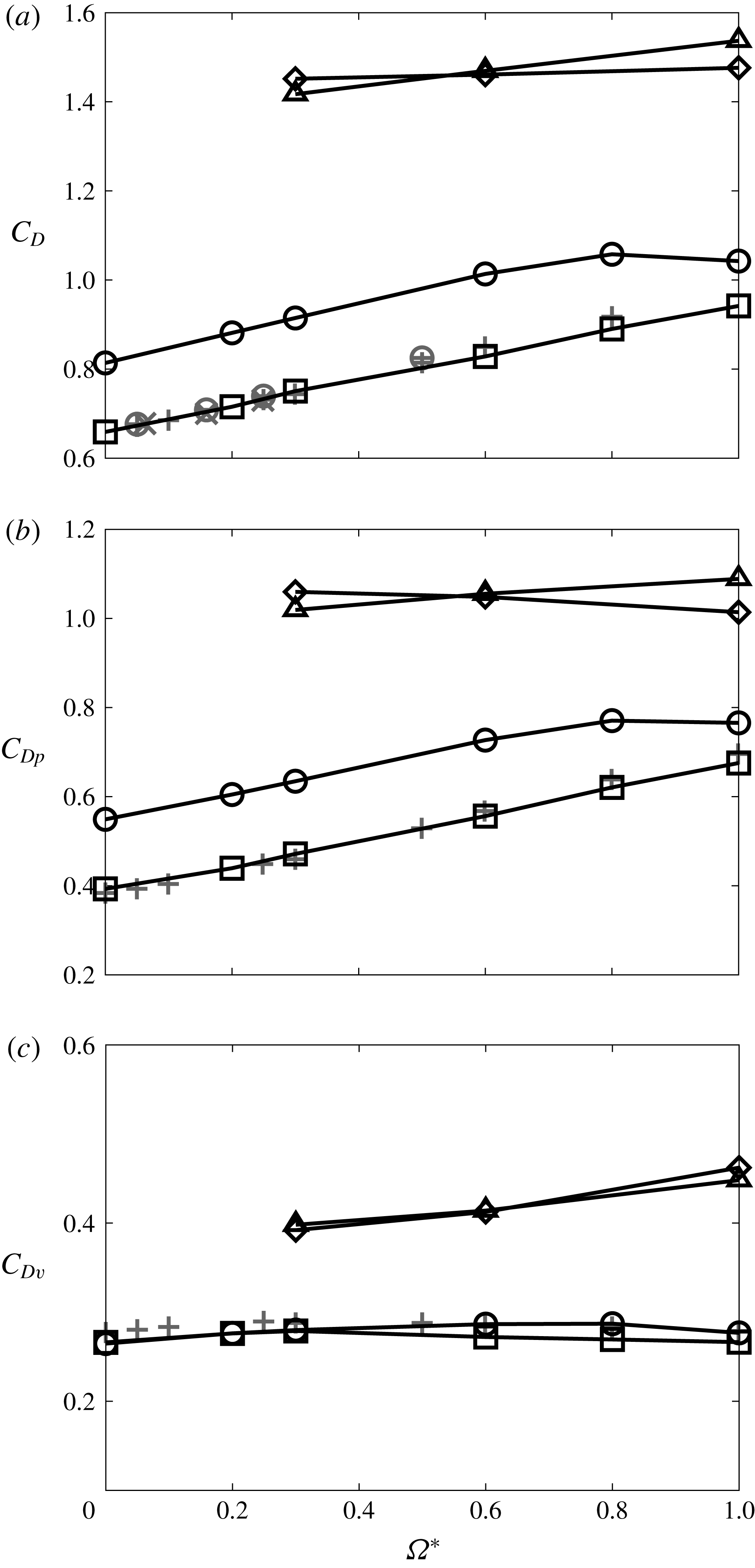
Figure 18. Time-averaged
 $C_{D}$
with respect to
$C_{D}$
with respect to
 $\unicode[STIX]{x1D6FA}^{\ast }$
at
$\unicode[STIX]{x1D6FA}^{\ast }$
at
 $Re=300$
: (
$Re=300$
: (
 $a$
) total; (
$a$
) total; (
 $b$
) pressure component; (
$b$
) pressure component; (
 $c$
) viscous component. Incompressible:
$c$
) viscous component. Incompressible:
 $M=0.3$
;
$M=0.3$
;  $M=0.8$
;
$M=0.8$
;  $M=1.2$
;
$M=1.2$
;  $M=2.0$
.
$M=2.0$
.
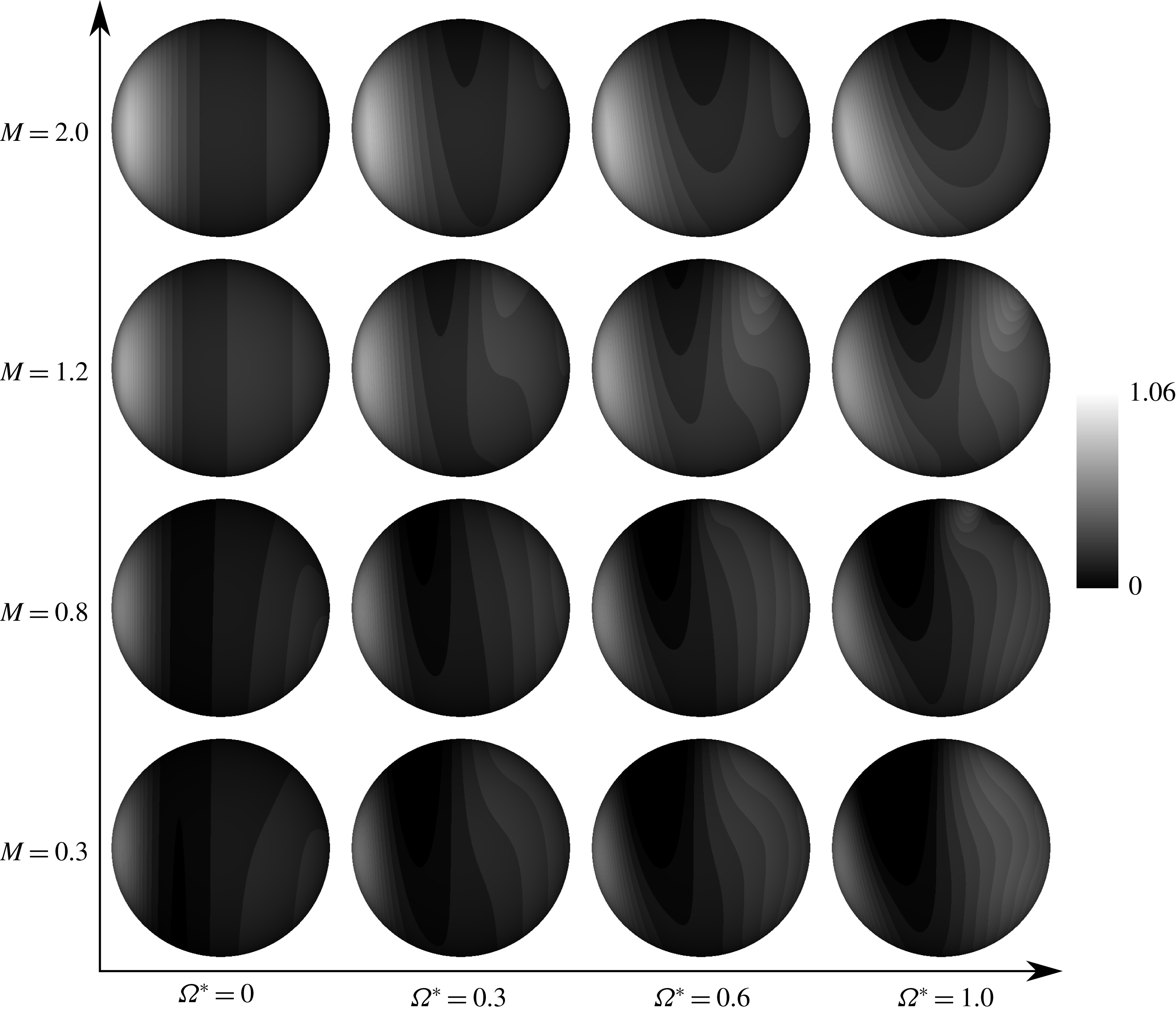
Figure 19. Distribution of the hydrodynamic stress coefficient in the drag force direction of a time-averaged field at
 $Re=300$
(view from
$Re=300$
(view from
 $-y$
).
$-y$
).
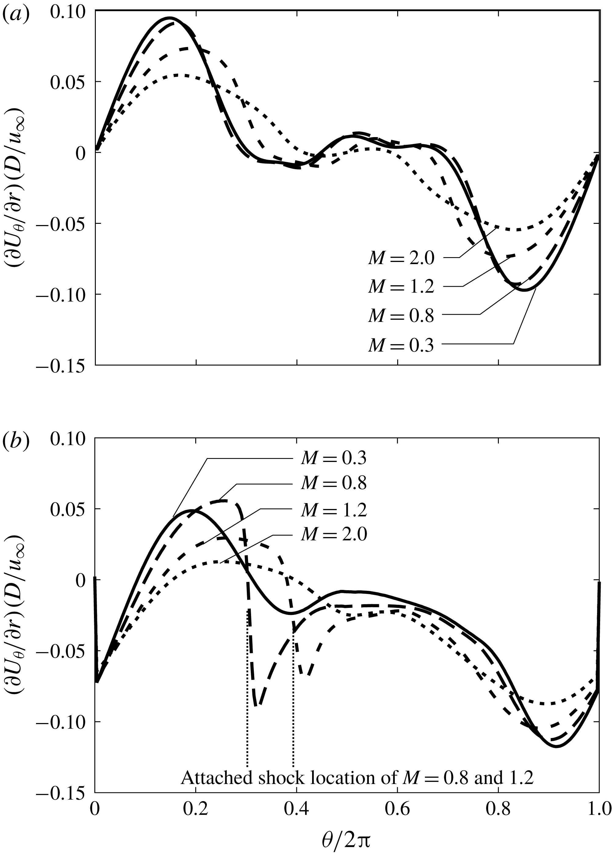
Figure 20. Normalized velocity gradient distribution at the surface of the sphere above the equator at
 $Re=300$
: (
$Re=300$
: (
 $a$
)
$a$
)
 $\unicode[STIX]{x1D6FA}^{\ast }=0.0$
; (
$\unicode[STIX]{x1D6FA}^{\ast }=0.0$
; (
 $b$
)
$b$
)
 $\unicode[STIX]{x1D6FA}^{\ast }=1.0$
.
$\unicode[STIX]{x1D6FA}^{\ast }=1.0$
.
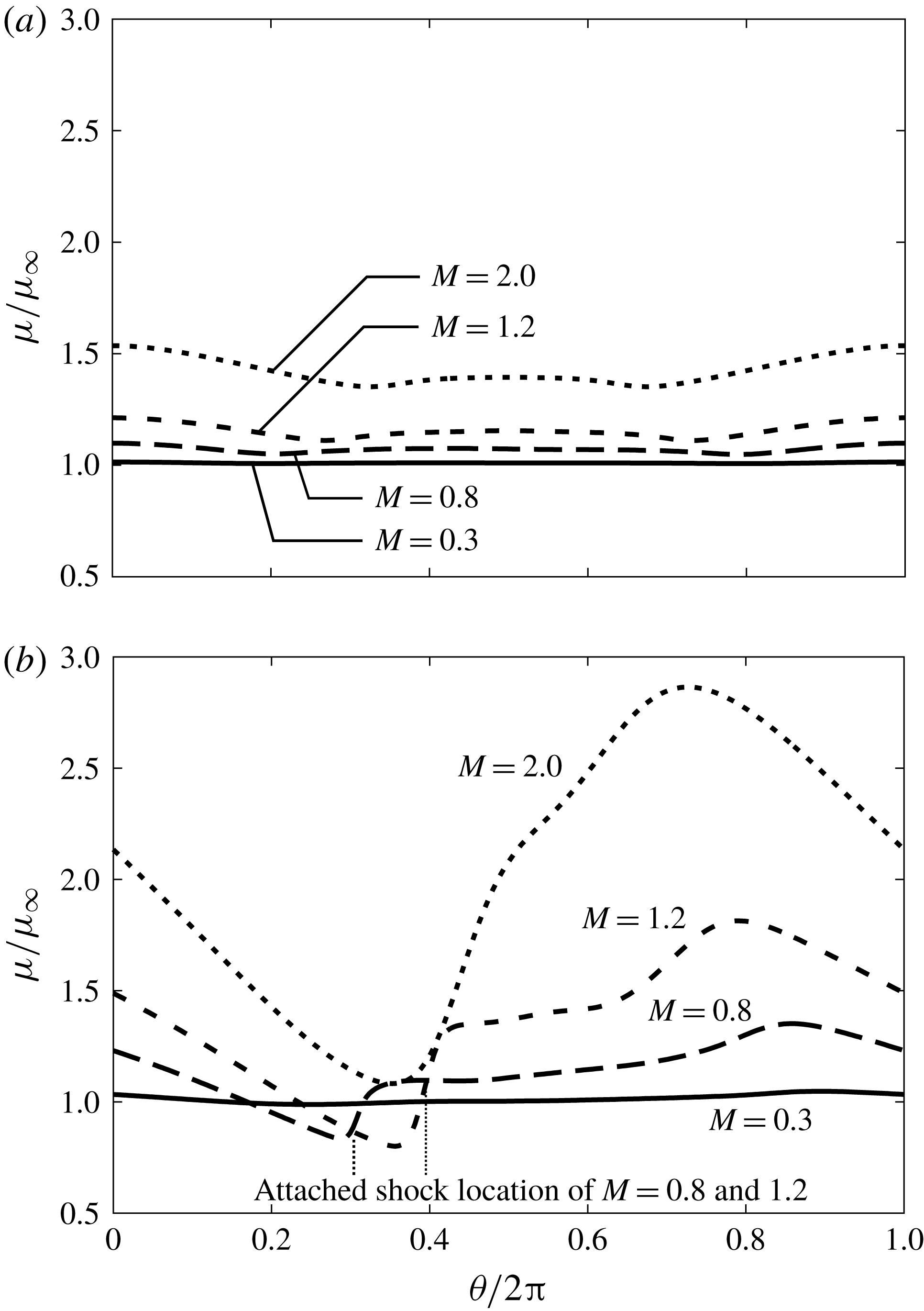
Figure 21. Normalized viscosity coefficient distribution at the surface of the sphere above the equator at
 $Re=300$
: (
$Re=300$
: (
 $a$
)
$a$
)
 $\unicode[STIX]{x1D6FA}^{\ast }=0.0$
; (
$\unicode[STIX]{x1D6FA}^{\ast }=0.0$
; (
 $b$
)
$b$
)
 $\unicode[STIX]{x1D6FA}^{\ast }=1.0$
.
$\unicode[STIX]{x1D6FA}^{\ast }=1.0$
.
Figure 19 shows the hydrodynamic stress distribution for the drag force direction in the time-averaged field. For figure 19, the drag force generated on the downstream side increases as
 $\unicode[STIX]{x1D6FA}^{\ast }$
increases, and its increment decreases as
$\unicode[STIX]{x1D6FA}^{\ast }$
increases, and its increment decreases as
 $M$
increases. On the other hand, the drag force generated on the upstream side decreases as
$M$
increases. On the other hand, the drag force generated on the upstream side decreases as
 $\unicode[STIX]{x1D6FA}^{\ast }$
increases, and its increment increases as
$\unicode[STIX]{x1D6FA}^{\ast }$
increases, and its increment increases as
 $M$
increases. These trends reflect the pressure coefficient distribution shown in figure 15. For supersonic flows, the free stream is decelerated at the detached shock wave. Hence, the effective rotation rate considered in the fluid velocity behind the detached shock wave and the rotation speed of the sphere are relatively fast compared with shock-free flows. The flow in the drag force direction is strongly reduced due to the stream generated by rotation of the sphere under supersonic flows. Also, the drag coefficient increases as
$M$
increases. These trends reflect the pressure coefficient distribution shown in figure 15. For supersonic flows, the free stream is decelerated at the detached shock wave. Hence, the effective rotation rate considered in the fluid velocity behind the detached shock wave and the rotation speed of the sphere are relatively fast compared with shock-free flows. The flow in the drag force direction is strongly reduced due to the stream generated by rotation of the sphere under supersonic flows. Also, the drag coefficient increases as
 $\unicode[STIX]{x1D6FA}^{\ast }$
increases due to the movement of the negative pressure region around
$\unicode[STIX]{x1D6FA}^{\ast }$
increases due to the movement of the negative pressure region around
 $\unicode[STIX]{x1D703}/\unicode[STIX]{x03C0}=0.7$
. These trends are similar, even if
$\unicode[STIX]{x1D703}/\unicode[STIX]{x03C0}=0.7$
. These trends are similar, even if
 $M$
increases, but the effect of
$M$
increases, but the effect of
 $\unicode[STIX]{x1D6FA}^{\ast }$
upon the pressure coefficient distribution is weaker under high-
$\unicode[STIX]{x1D6FA}^{\ast }$
upon the pressure coefficient distribution is weaker under high-
 $M$
conditions. Also, the pressure coefficient distribution itself drastically changes as
$M$
conditions. Also, the pressure coefficient distribution itself drastically changes as
 $M$
increases. In addition, the decrease (increase) of the pressure coefficient in the region around the
$M$
increases. In addition, the decrease (increase) of the pressure coefficient in the region around the
 $\unicode[STIX]{x1D703}/\unicode[STIX]{x03C0}=0.0$
–0.25 (
$\unicode[STIX]{x1D703}/\unicode[STIX]{x03C0}=0.0$
–0.25 (
 $\unicode[STIX]{x1D703}/\unicode[STIX]{x03C0}=0.5$
–0.75) side caused by rotation increases (decreases) as
$\unicode[STIX]{x1D703}/\unicode[STIX]{x03C0}=0.5$
–0.75) side caused by rotation increases (decreases) as
 $M$
increases. For this behaviour, the increase of the drag coefficient due to rotation becomes small under high-
$M$
increases. For this behaviour, the increase of the drag coefficient due to rotation becomes small under high-
 $M$
conditions.
$M$
conditions.
The viscous drag coefficient,
 $C_{Dv}$
, is hardly changed by rotation for subsonic cases. On the other hand,
$C_{Dv}$
, is hardly changed by rotation for subsonic cases. On the other hand,
 $C_{Dv}$
increases as
$C_{Dv}$
increases as
 $\unicode[STIX]{x1D6FA}^{\ast }$
increases because the friction stress increases on the advancing side due to change of the velocity gradient and the viscosity coefficient at the surface of the sphere in the supersonic cases. The viscous drag coefficient increases as
$\unicode[STIX]{x1D6FA}^{\ast }$
increases because the friction stress increases on the advancing side due to change of the velocity gradient and the viscosity coefficient at the surface of the sphere in the supersonic cases. The viscous drag coefficient increases as
 $\unicode[STIX]{x1D6FA}^{\ast }$
increases under supersonic flow. Figure 20 shows the velocity gradient distribution of the
$\unicode[STIX]{x1D6FA}^{\ast }$
increases under supersonic flow. Figure 20 shows the velocity gradient distribution of the
 $\unicode[STIX]{x1D703}$
-direction velocity
$\unicode[STIX]{x1D703}$
-direction velocity
 $U_{\unicode[STIX]{x1D703}}$
for the
$U_{\unicode[STIX]{x1D703}}$
for the
 $r$
direction on the surface of the sphere above the equator, which is normalized by the free-stream velocity and the diameter of the sphere. For figure 20, the velocity gradient decreases as
$r$
direction on the surface of the sphere above the equator, which is normalized by the free-stream velocity and the diameter of the sphere. For figure 20, the velocity gradient decreases as
 $\unicode[STIX]{x1D6FA}^{\ast }$
increases in most areas of the retreating and advancing sides. This trend is similar between subsonic and supersonic flows, but under the supersonic condition, change in the velocity gradient distribution due to rotation is affected by shock waves. For example, the sign of the velocity gradient changes sharply around
$\unicode[STIX]{x1D6FA}^{\ast }$
increases in most areas of the retreating and advancing sides. This trend is similar between subsonic and supersonic flows, but under the supersonic condition, change in the velocity gradient distribution due to rotation is affected by shock waves. For example, the sign of the velocity gradient changes sharply around
 $\unicode[STIX]{x1D703}/\unicode[STIX]{x03C0}=0.25$
by an attached shock wave for
$\unicode[STIX]{x1D703}/\unicode[STIX]{x03C0}=0.25$
by an attached shock wave for
 $M=0.8$
and 1.2. Also, the shock wave moves downstream as
$M=0.8$
and 1.2. Also, the shock wave moves downstream as
 $M$
increases. For
$M$
increases. For
 $M=0.3$
, the velocity gradient in most of the retreating side is positive, so the friction stress at the retreating side acts to promote rotation. Conversely, for
$M=0.3$
, the velocity gradient in most of the retreating side is positive, so the friction stress at the retreating side acts to promote rotation. Conversely, for
 $M\geqslant 0.8$
, the region with a negative velocity gradient on the retreating side is expanded by the effect of attached shock waves. Moreover, for
$M\geqslant 0.8$
, the region with a negative velocity gradient on the retreating side is expanded by the effect of attached shock waves. Moreover, for
 $M\geqslant 1.2$
, the peak velocity gradient on the retreating side becomes small as
$M\geqslant 1.2$
, the peak velocity gradient on the retreating side becomes small as
 $M$
increases. This trend is caused by the influence of the detached shock wave, which decelerates the fluid around the sphere. For this influence, the relative velocity between the surface of the sphere and the free stream becomes small as
$M$
increases. This trend is caused by the influence of the detached shock wave, which decelerates the fluid around the sphere. For this influence, the relative velocity between the surface of the sphere and the free stream becomes small as
 $M$
increases. The viscosity coefficient distribution on the surface of the sphere above the equator is shown in figure 21. Under the influence of rotation, the viscosity coefficient decreases (increases) at the retreating (advancing) side. Also, the velocity gradient at the surface of the sphere on the retreating (advancing) side becomes small (large), due to the influence of rotation. Hence, the viscous drag and moment coefficient are larger than in stationary cases for high-
$M$
increases. The viscosity coefficient distribution on the surface of the sphere above the equator is shown in figure 21. Under the influence of rotation, the viscosity coefficient decreases (increases) at the retreating (advancing) side. Also, the velocity gradient at the surface of the sphere on the retreating (advancing) side becomes small (large), due to the influence of rotation. Hence, the viscous drag and moment coefficient are larger than in stationary cases for high-
 $M$
and high-
$M$
and high-
 $\unicode[STIX]{x1D6FA}^{\ast }$
conditions. The viscous coefficient mainly increases around the stagnation point upstream behind the attached shock wave and the advancing side downstream due to rotation. The effects of the shock waves become strong as
$\unicode[STIX]{x1D6FA}^{\ast }$
conditions. The viscous coefficient mainly increases around the stagnation point upstream behind the attached shock wave and the advancing side downstream due to rotation. The effects of the shock waves become strong as
 $M$
increases. Also, large aerodynamic heating occurs on the advancing side because the relative velocity on the advancing side between fluid and surface is larger than that of the retreating side. Thus, the viscosity coefficient on the advancing side increases remarkably under the high-
$M$
increases. Also, large aerodynamic heating occurs on the advancing side because the relative velocity on the advancing side between fluid and surface is larger than that of the retreating side. Thus, the viscosity coefficient on the advancing side increases remarkably under the high-
 $M$
condition for rotating cases.
$M$
condition for rotating cases.
5.3 Moment coefficient around the rotation axis
Figure 22 shows moment coefficients around the rotation axis: compressibility effects appear in the moment coefficient. In rotating cases, the moment coefficient has a negative value, meaning that moment opposes the rotation of the sphere and its strength increases along with
 $\unicode[STIX]{x1D6FA}^{\ast }$
. Also, the increment of the moment coefficient by rotation becomes large as
$\unicode[STIX]{x1D6FA}^{\ast }$
. Also, the increment of the moment coefficient by rotation becomes large as
 $M$
increases, and this effect increases along with Re.
$M$
increases, and this effect increases along with Re.
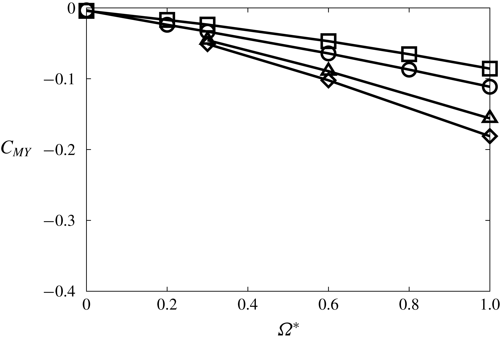
Figure 22. Moment coefficients around the rotation axis at
 $Re=300$
:
$Re=300$
:
 $M=0.3$
;
$M=0.3$
;  $M=0.8$
;
$M=0.8$
;  $M=1.2$
;
$M=1.2$
;  $M=2.0$
.
$M=2.0$
.
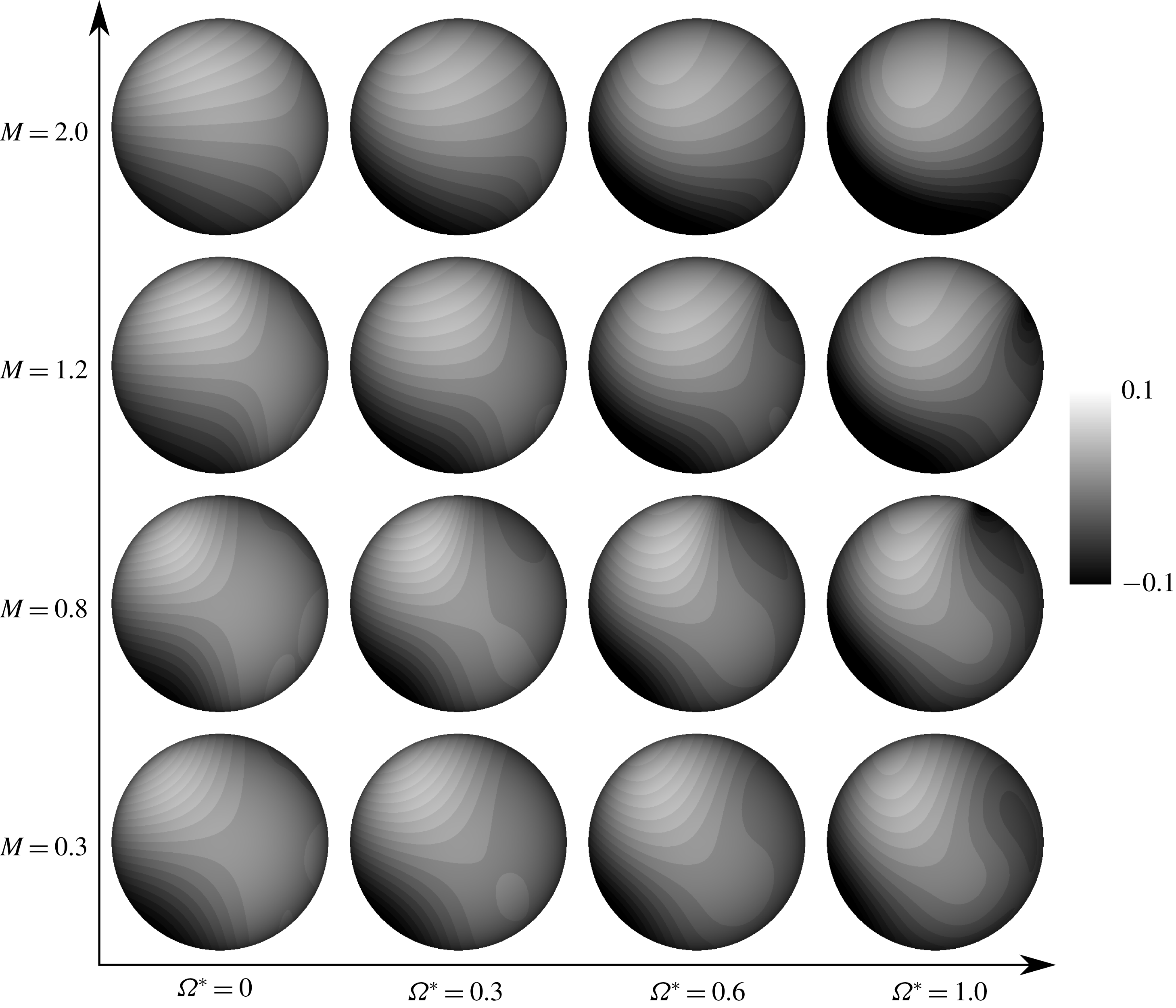
Figure 23. Distribution of the y-direction local moment coefficient of hydrodynamic stress in a time-averaged field at
 $Re=300$
(view from
$Re=300$
(view from
 $-y$
).
$-y$
).
Figure 23 shows the local moment coefficient distribution. This coefficient is calculated as the product of hydrodynamic stress tangential to the surface for the
 $\unicode[STIX]{x1D709}$
direction and the moment arm, and is normalized by the diameter of the sphere and the dynamic pressure based on the free-stream quantities. In stationary cases, the moment around the rotation axis acts symmetrically on the retreating and advancing sides. However, as
$\unicode[STIX]{x1D709}$
direction and the moment arm, and is normalized by the diameter of the sphere and the dynamic pressure based on the free-stream quantities. In stationary cases, the moment around the rotation axis acts symmetrically on the retreating and advancing sides. However, as
 $\unicode[STIX]{x1D6FA}^{\ast }$
increases, the local moment coefficient distribution becomes asymmetric. Thus, the relative fluid velocity between the vicinity of the sphere and the surface of the sphere on the retreating (advancing) side becomes small (large) as
$\unicode[STIX]{x1D6FA}^{\ast }$
increases, the local moment coefficient distribution becomes asymmetric. Thus, the relative fluid velocity between the vicinity of the sphere and the surface of the sphere on the retreating (advancing) side becomes small (large) as
 $\unicode[STIX]{x1D6FA}^{\ast }$
increases. Also, the difference between the absolute value of the local moment coefficient on the retreating and advancing sides becomes large as
$\unicode[STIX]{x1D6FA}^{\ast }$
increases. Also, the difference between the absolute value of the local moment coefficient on the retreating and advancing sides becomes large as
 $M$
increases. On the retreating side, the local moment coefficient in supersonic flows is smaller than that of subsonic flows for the same
$M$
increases. On the retreating side, the local moment coefficient in supersonic flows is smaller than that of subsonic flows for the same
 $\unicode[STIX]{x1D6FA}^{\ast }$
, because the relative velocity between the surface of the sphere and the fluid in its vicinity is smaller than under subsonic conditions. This is due to the deceleration of the fluid velocity at the detached shock wave. Conversely, on the advancing side, the local moment coefficient for high-
$\unicode[STIX]{x1D6FA}^{\ast }$
, because the relative velocity between the surface of the sphere and the fluid in its vicinity is smaller than under subsonic conditions. This is due to the deceleration of the fluid velocity at the detached shock wave. Conversely, on the advancing side, the local moment coefficient for high-
 $M$
flow is larger than that of the low-
$M$
flow is larger than that of the low-
 $M$
flow due to the increase of the viscosity coefficient, as shown in figure 21. Also, the negative local moment coefficient appears on the retreating side for
$M$
flow due to the increase of the viscosity coefficient, as shown in figure 21. Also, the negative local moment coefficient appears on the retreating side for
 $M=0.8$
and 1.2 under the influence of the attached shock wave. By forming this shock wave on the retreating side, the fluid in the vicinity of the sphere is decelerated. Therefore, the friction stress on the surface behind the attached shock wave increases due to the increase of the velocity gradient and the viscosity coefficient, and its effect becomes large as
$M=0.8$
and 1.2 under the influence of the attached shock wave. By forming this shock wave on the retreating side, the fluid in the vicinity of the sphere is decelerated. Therefore, the friction stress on the surface behind the attached shock wave increases due to the increase of the velocity gradient and the viscosity coefficient, and its effect becomes large as
 $M$
and
$M$
and
 $\unicode[STIX]{x1D6FA}^{\ast }$
increase. Thus, the attached shock wave formed on the retreating side has a braking effect on particle rotation. From the above results, in the case of compressible flow, particle rotation is easy to stop compared with incompressible flows.
$\unicode[STIX]{x1D6FA}^{\ast }$
increase. Thus, the attached shock wave formed on the retreating side has a braking effect on particle rotation. From the above results, in the case of compressible flow, particle rotation is easy to stop compared with incompressible flows.
Table 2. Summary of effect of
 $\unicode[STIX]{x1D6FA}^{\ast }$
and
$\unicode[STIX]{x1D6FA}^{\ast }$
and
 $M$
on each parameter.
$M$
on each parameter.
A summary of the effects of
 $\unicode[STIX]{x1D6FA}^{\ast }$
on
$\unicode[STIX]{x1D6FA}^{\ast }$
on
 $C_{L}$
,
$C_{L}$
,
 $C_{D}$
,
$C_{D}$
,
 $C_{MY}$
and St and the effects of
$C_{MY}$
and St and the effects of
 $M$
on the increment of
$M$
on the increment of
 $C_{L}$
,
$C_{L}$
,
 $C_{D}$
,
$C_{D}$
,
 $C_{MY}$
and St due to rotation is shown in table 2. The
$C_{MY}$
and St due to rotation is shown in table 2. The
 $\unicode[STIX]{x1D6FA}^{\ast }$
effect on each parameter is the same between the incompressible and compressible flows. The increment of
$\unicode[STIX]{x1D6FA}^{\ast }$
effect on each parameter is the same between the incompressible and compressible flows. The increment of
 $C_{L}$
and
$C_{L}$
and
 $C_{D}$
becomes small as
$C_{D}$
becomes small as
 $M$
increases. On the other hand, the increment of
$M$
increases. On the other hand, the increment of
 $C_{MY}$
becomes small as
$C_{MY}$
becomes small as
 $M$
increases. Also, the increment of St is not influenced by
$M$
increases. Also, the increment of St is not influenced by
 $M$
.
$M$
.
6 Conclusions
In this study, direct numerical simulation of flow around a rotating sphere in the subsonic to supersonic regime at
 $100\leqslant Re\leqslant 300$
is undertaken by solving the three-dimensional compressible Navier–Stokes equations. As a result, we clarified the differences in flow properties between the incompressible and compressible flows. The vortex structure behind the sphere is influenced by Re,
$100\leqslant Re\leqslant 300$
is undertaken by solving the three-dimensional compressible Navier–Stokes equations. As a result, we clarified the differences in flow properties between the incompressible and compressible flows. The vortex structure behind the sphere is influenced by Re,
 $\unicode[STIX]{x1D6FA}^{\ast }$
and
$\unicode[STIX]{x1D6FA}^{\ast }$
and
 $M$
. In particular, vortex shedding is significantly reduced in supersonic flows. Also, under the subsonic and high-
$M$
. In particular, vortex shedding is significantly reduced in supersonic flows. Also, under the subsonic and high-
 $\unicode[STIX]{x1D6FA}^{\ast }$
conditions, the compressibility effect on the vortex structure appears strongly compared with stationary cases, because the fluid velocity and the relative velocity between the fluid and the surface of the sphere is large on the retreating and advancing sides, respectively.
$\unicode[STIX]{x1D6FA}^{\ast }$
conditions, the compressibility effect on the vortex structure appears strongly compared with stationary cases, because the fluid velocity and the relative velocity between the fluid and the surface of the sphere is large on the retreating and advancing sides, respectively.
The lift force caused by rotation becomes large as
 $\unicode[STIX]{x1D6FA}^{\ast }$
increases for each
$\unicode[STIX]{x1D6FA}^{\ast }$
increases for each
 $M$
. However, the increment of the lift coefficient becomes small as
$M$
. However, the increment of the lift coefficient becomes small as
 $M$
increases. This is caused by deceleration of the fluid velocity by attached shock waves formed on the retreating side. Also, the position of the stagnation point formed at the advancing side is influenced by
$M$
increases. This is caused by deceleration of the fluid velocity by attached shock waves formed on the retreating side. Also, the position of the stagnation point formed at the advancing side is influenced by
 $M$
, and moves downstream as
$M$
, and moves downstream as
 $M$
increases. Hence, the lift force caused by rotation becomes small as
$M$
increases. Hence, the lift force caused by rotation becomes small as
 $M$
increases. In addition, the moment coefficient around the rotation axis, which brakes rotation, increases along with
$M$
increases. In addition, the moment coefficient around the rotation axis, which brakes rotation, increases along with
 $M$
due to the effect of the attached shock wave formed on the retreating side. These results mean that the effect of the particle rotation on the lift coefficient under compressible flows is smaller than that of the incompressible flows.
$M$
due to the effect of the attached shock wave formed on the retreating side. These results mean that the effect of the particle rotation on the lift coefficient under compressible flows is smaller than that of the incompressible flows.
Acknowledgements
The present simulations were implemented on the supercomputer of the Japan Aerospace Exploration Agency. This work was supported by JSPS KAKENHI grant nos 17K06167 and 18J11205.
Appendix. Validation and verification
The results of the validation and verification studies are shown in table 3. In the grid-size- and domain-size-independent tests, the number of grid points in each direction and the size of the computational domain are 1.29 and 1.5 times the baseline grid, respectively. As a result, the hydrodynamic force coefficients are not influenced by the grid and domain sizes.
Figure 24. Comparisons of
 $C_{L}$
time history of modified WENOCU6-FP and original WENOCU6-FP (
$C_{L}$
time history of modified WENOCU6-FP and original WENOCU6-FP (
 $Re=300$
,
$Re=300$
,
 $M=0.3$
and
$M=0.3$
and
 $\unicode[STIX]{x1D6FA}=1.0$
).
$\unicode[STIX]{x1D6FA}=1.0$
).
Table 3. Comparison of hydrodynamic force coefficient.
In addition, in this study, the central difference component of WENOCU6-FP is replaced by one of the splitting type proposed by Pirozzoli (Reference Pirozzoli2011), in order to stabilize the calculation. In the replaced WENOCU6-FP, the numerical viscosity is introduced only by the dissipation term for the sixth-order WENOCU, and such an approach is originally used by Yee, Sandham & Djomehri (Reference Yee, Sandham and Djomehri1999). Also, it has been confirmed that this splitting-type scheme gives an accurate and stable solution over conventional central discretization by numerical tests using the central difference scheme (Pirozzoli Reference Pirozzoli2011). To confirm that influence, the hydrodynamic force coefficients by the original WENOCU6-FP is also shown in table 1. In addition, the time history of
 $C_{L}$
and instantaneous
$C_{L}$
and instantaneous
 $C_{P}$
distribution are shown in figures 24 and 25, respectively. Note that the simulation using the original WENOCU6-FP blows up as shown in figure 24. Therefore, the hydrodynamic force coefficients shown in table 3 might not be reliable. However, the
$C_{P}$
distribution are shown in figures 24 and 25, respectively. Note that the simulation using the original WENOCU6-FP blows up as shown in figure 24. Therefore, the hydrodynamic force coefficients shown in table 3 might not be reliable. However, the
 $C_{P}$
distribution before blowing up is very similar.
$C_{P}$
distribution before blowing up is very similar.
Figure 25. Comparisons of
 $C_{P}$
distribution of modified WENOCU6-FP and original WENOCU6-FP (before blowing up) for
$C_{P}$
distribution of modified WENOCU6-FP and original WENOCU6-FP (before blowing up) for
 $Re=300$
,
$Re=300$
,
 $M=0.3$
and
$M=0.3$
and
 $\unicode[STIX]{x1D6FA}=1.0$
.
$\unicode[STIX]{x1D6FA}=1.0$
.


