


1. Introduction
In coastal flows, free-surface waves approaching the shore will typically grow in amplitude until they eventually break. The mathematical theory behind this phenomenon is known as shoaling (see e.g. the review by Meyer Reference Meyer1979). For a typical situation where the dynamics are primarily governed by a two-dimensional flow (e.g. in a direction perpendicular to the coastline), we are interested in the evolution of the waves as a function of the distance of propagation. We provide in figure 1 a typical set-up of a numerical or experimental wave flume used to model such coastal flows.

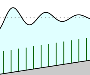
Figure 1. Schematic diagram of a wave flume with waves propagating from left to right. Sample solutions of the free-surface elevation,  $\eta$, are plotted as functions of distance of propagation at various times – this is to highlight the slow modulation of the wave due both the vegetative canopy and the varying substrate.
We consider, as the simplest example, a monochromatic problem. Then in a suitably non-dimensionalised form, the leading-order free surface,  $\eta$, might be approximated by
  $\eta \sim A(x) \cos (\varPhi (x)/\alpha - t)$ where
  $x$ is distance in the direction of propagation,
  $t$ is time,
  $A$ is the wave amplitude and
  $\varPhi (x)/\alpha$ is the phase. If the wavelength is small by comparison with the length scale over which the amplitude varies (quantified by the assumption that
  $\alpha$ is small) it is possible to average the effects of drag and varying topography over a wave period to derive a differential equation for
  $A$ of the form
 \begin{equation} \frac{\mathrm{d} A}{\mathrm{d} x} = \mathcal{F}(x, A(x), \text{vegetative parameters}, \text{substrate parameters}). \end{equation}
Our goal in this work is to derive such an equation for waves over rigid vegetation with varying substrate.
1.1. Oscillatory flows through vegetation
There is great diversity in terms of regimes and scenarios in oscillatory flows through vegetation, which has led to a substantial number of studies. For example, experiments with wave flumes as well as field studies can be used to understand the effects of canopy arrangement and foliage – we refer the reader to reviews and work by, for example, Bradley & Houser (Reference Bradley and Houser2009), Anderson & Smith (Reference Anderson and Smith2014), Möller et al. (Reference Möller2014) and Lei & Nepf (Reference Lei and Nepf2019). On the other hand, numerical simulations can be done to investigate effects such as turbulence of the in-canopy flow and related issues such as sediment transportation – we refer to the detailed reviews of Lowe, Koseff & Monismith (Reference Lowe, Koseff and Monismith2005) and Zeller et al. (Reference Zeller, Zarama, Weitzman and Koseff2015), and also individual works by Suzuki et al. (Reference Suzuki, Zijlema, Burger, Meijer and Narayan2012), Liu et al. (Reference Liu, Chang, Mei, Lomonaco, Martin and Maza2015) and Mattis et al. (Reference Mattis, Kees, Wei, Dimakopoulos and Dawson2019).
A theoretical analysis can also be practically useful by giving predictions in a greater parameter space, based on careful assumptions or simplifications (Nepf Reference Nepf2012). In particular, the ability to predict how a wave evolves along a given domain can be used for applications such as coastal management (Morris et al. Reference Morris, Konlechner, Ghisalberti and Swearer2018). Much of the work on analytical approaches has been devoted to the development of energy balance arguments. For example, Dalrymple, Kirby & Hwang (Reference Dalrymple, Kirby and Hwang1984) and Kobayashi, Raichle & Asano (Reference Kobayashi, Raichle and Asano1993) applied energetic balances in order to derive equations of the form (1.1) for the case of rigid vegetation over horizontal substrates. These predictions were extended by Mendez & Losada (Reference Mendez and Losada2004) to random waves and also shallow-water waves over uniformly sloping beaches – such predictions have been widely used in the engineering community (see e.g. Luhar, Infantes & Nepf (Reference Luhar, Infantes and Nepf2017) and the references therein).
In this article, we extend previous analyses by giving a systematic asymptotic reduction of a free-surface wave travelling over vegetation on a general slowly varying substrate, where all the forces which act on the vegetation are considered. The systematic multiple-scales approach we adopt has the advantage of formally quantifying the accuracy of the approximations made, while allowing more easily the systematic inclusion of multiple physical effects, including the combination of varying bathymetry and vegetation resulting in both frequency and amplitude modulation.
Our analysis is motivated by the seminal work of Keller (Reference Keller1958), who studied three-dimensional flows over slowly varying substrate profiles using linear wave theory and ray theory. By considering the asymptotic limit in which the water depth and the wavelength are both much smaller than the horizontal scale of the substrate contour, a Wentzel–Kramers–Brillouin (WKB) (or Liouville–Green) approximation explained how the wave amplitude and phase would slowly modulate as the wave propagates. The aim of this work is to extend this analysis by accounting for the presence of vegetation.
The method of multiple scales has been successfully applied to the problem of vegetative flows in a series of recent papers by Mei et al. (Reference Mei, Chan, Liu, Huang and Zhang2011), Mei, Chan & Liu (Reference Mei, Chan and Liu2014) and Wang, Guo & Mei (Reference Wang, Guo and Mei2015). In the first two references, shallow-water waves and intermediate-depth waves over emergent vegetation are analysed. The more recent work by Wang et al. (Reference Wang, Guo and Mei2015) considers waves over a shallow canopy. In all three approaches, the in-canopy flow is solved in detail with finite elements. The regime studied in these works is rather different to that of the current study.
The analysis in Wang et al. (Reference Wang, Guo and Mei2015) considers the shallow-canopy regime where the canopy height is comparable to the width and separation of the plants, and is much smaller than the wavelength (which is also comparable to the water depth). The in-canopy flow is then formally depth-averaged and solved numerically over a unit cell, accounting for bed shear and turbulence, providing a linear effective boundary condition on the irrotational flow above. The small scale in their multiple-scales analysis is the plant separation, while the large scale is the wavelength of the incoming wave.
In the present work we treat the regime in which the submerged canopy occupies a finite fraction of the water depth. Such a scenario is much more challenging to attack using the approach of Wang et al. (Reference Wang, Guo and Mei2015), so we simplify in other ways. We consider the limit in which the plant size is much smaller than the plant separation, which allows individual plants to be treated as line momentum sinks. These are then formally homogenised to directly model the canopy-induced momentum loss with Morison's formula (accounting for drag, added mass and virtual buoyancy) (Dean & Dalrymple Reference Dean and Dalrymple1991). We then use a generalisation of the method of multiple scales in which the small scale is the wavelength of the wave, and the large scale is the decay length of the wave amplitude. Essentially Wang et al. (Reference Wang, Guo and Mei2015) consider the regime in which the plant height  $\sim$ plant width
  $\sim$ plant separation
  $\ll$ wavelength
  $\sim$ water depth, while we consider the regime in which the plant width
  $\ll$ plant separation
  $\ll$ plant height
  $\sim$ wavelength
  $\sim$ water depth.
In summary, we provide a systematic asymptotic reduction of a free-surface wave travelling over vegetation on a varying substrate. In particular, our analysis and resulting analytical predictions account for:
(i) waves of arbitrary wavelengths;
(ii) phase shift of the wave as it propagates;
(iii) the role of various forces which act on individual plants (drag, added mass and virtual buoyancy);
(iv) variation of the canopy along the direction of wave propagation.
1.2. Structure of this work
We first present in § 2 the governing equations of the fluid and the continuum modelling framework for the vegetation. By exploiting the slowly varying nature of waves along the domain, we apply in § 3 a generalised multiple-scales analysis developed by Kuzmak (Reference Kuzmak1959) to systematically derive the equation for the wave amplitude. We demonstrate in § 4 that our results agree with previous analyses for particular limiting cases. We validate our asymptotic predictions in §§ 5–6 with full two-phase numerical simulations and experimental data from previous studies. In a continuation of this article, we explore the problem of wave evolution in the presence of flexible vegetation.
2. Theoretical formulation
In this section, we use hats ( $\hat {\cdot }$) to denote variables which are dimensional – we will drop the hats when we non-dimensionalise the problem. We consider an inviscid fluid with velocity
  $\hat {\boldsymbol {u}}=(\hat {u},\hat {v},\hat {w})$ that flows over a canopy region of finite depth (see figure 2). We assume that the canopy is fully submerged and covers the entire substrate. Within the canopy, we model individual plants as rigid upright beams of width
  $b$ and length
  $\hat {h}$. However, we note that it is impractical to monitor the contributions of individual plants. Instead, following the analysis in Wong, Trinh & Chapman (Reference Wong, Trinh and Chapman2020), we consider a simpler averaged model in which the canopy is an effective medium that contributes a bulk volumetric drag.

Figure 2. Schematic diagram of waves with fluid velocity  $\hat {\boldsymbol {u}}$ propagating through a rigid canopy over a varying substrate with
  $\hat {z}=-\hat {H}$. The free-surface elevation is parameterised with
  $\hat {z}=\hat {\eta }$ and the submerged green obstacles represent individual plants with height
  $\hat {h}$.
One immediate benefit of this homogenisation is that it allows us to consider a flow in which the geometry and initial conditions are independent of the transverse direction  $\hat {y}$, allowing solutions which are two-dimensional (i.e. functions of
  $\hat {x}$,
  $\hat {z}$ and
  $\hat {t}$ only) with
  $\hat {v}=0$, which we henceforth assume. Consider, therefore, an inviscid flow in a domain of finite depth bounded below by a variable bottom substrate,
  $\hat {z} = -\hat {H}(\hat {x})$, and above by a free surface,
  $\hat {z} = \hat {\eta }(\hat {x},\hat {t})$. We assume a monochromatic incident wave propagating in the positive
  $\hat {x}$-direction. A schematic of the two-dimensional set-up is given in figure 3.

Figure 3. Schematic diagram of waves propagating through a canopy over a varying substrate with  $\hat {z}=-\hat {H}(\hat {x})$. The waves propagate along the
  $\hat {x}$-direction, with the free surface being parameterised with
  $\hat {z}=\hat {\eta }(\hat {x},\hat {t})$. The green obstacles along the substrate represent individual plants with width
  $b$ and length
  $\hat {h}$.
From the Euler equations, the fluid velocity satisfies
 $$\begin{gather} \boldsymbol{\nabla}\boldsymbol{\cdot} \hat{\boldsymbol{u}} = 0, \end{gather}$$
 $$\begin{gather}\rho\left(\frac{\partial \hat{\boldsymbol{u}}}{\partial \hat{t}}+\boldsymbol{\hat{u}}\boldsymbol{\cdot}\boldsymbol{\nabla} \hat{\boldsymbol{u}}\right) ={-}\boldsymbol{\nabla} \hat{\tilde{p}}-\hat{\bar{\boldsymbol{F}}}, \end{gather}$$
where the density  $\rho$ is taken to be constant. Here we have defined
  $\hat {\tilde {p}}=\hat {\tilde {p}}_{{static}}-\rho g \hat {z}$ to be the dynamic pressure, where
  $g$ is the acceleration due to gravity; use of the dynamic pressure simplifies the implementation of both analytical and numerical methods. The additional sink term,
  $\hat {\bar {\boldsymbol {F}}}$, in the momentum equation (2.1b) incorporates the effects of the canopy.
In considering the force balance on rigid and static objects submerged in a fluid, we must account for drag, added mass and virtual buoyancy (Gosselin Reference Gosselin2019). With  $\bar {N}$ the number of plants planted per unit area (along the substrate) and
  ${H}$ the Heaviside function, the bulk volumetric sink term
  $\hat {\bar {\boldsymbol {F}}}$ is given by
 \begin{equation} \hat{\bar{\boldsymbol{F}}}=\bar{N}{H}(\hat{h}-\hat{H}-\hat{z}) \hat{\boldsymbol{F}}, \end{equation}
where  $\hat {h}(\hat {x})$ is the height of the canopy and the component forces from the individual beams are given by
 \begin{equation} \hat{\boldsymbol{F}} = \hat{\boldsymbol{F}}_D \ \text{(drag)} + \hat{\boldsymbol{F}}_A \ \text{(added mass)} + \hat{\boldsymbol{F}}_V \ (\text{virtual buoyancy}); \end{equation}
the Heaviside function ensures that momentum is only lost within the canopy. Following previous analyses on submerged beams by Luhar & Nepf (Reference Luhar and Nepf2016) and Leclercq & de Langre (Reference Leclercq and de Langre2018), we set
 \begin{equation} \hat{\boldsymbol{F}}_D = \frac{1}{2}\rho bC_D \hat{u}\left|\hat{u}\right|\hat{\boldsymbol{e}}_{\hat{x}}, \quad \hat{\boldsymbol{F}}_{A} = \rho \mathcal{A} C_M\frac{\partial \hat{u}}{\partial \hat{t}}\hat{\boldsymbol{e}}_{\hat{x}}, \quad \hat{\boldsymbol{F}}_V=\rho\mathcal{A}\frac{\partial \hat{\boldsymbol{u}}}{\partial \hat{t}}. \end{equation}
In the expressions above,  $\mathcal {A}$ is the cross-sectional area of a plant perpendicular to the
  $z$-axis,
  $C_D$ is the drag coefficient and
  $C_M$ is the added mass coefficient.
2.1. Non-dimensionalisation
We non-dimensionalise using the following scales:
 \begin{equation} [\hat{\boldsymbol{x}}]=L,\quad [\hat{\eta}]=A_0, \quad [\hat{t}] = \omega_0^{{-}1}, \quad [\hat{\boldsymbol{u}}]= A_0\omega_0, \quad [\hat{p}] = \rho g A_0, \end{equation}
where  $\omega _0$,
  $A_0$ are the wave frequency and initial amplitude, and
  $L$ is the horizontal length scale of the domain, which will be made precise in § 3. Note that we non-dimensionalise lengths with the
  $L$, rather than the depth or the wavelength; this is for convenience of the forthcoming multiple-scales analysis in § 3. Note also that we have chosen to scale the velocity with the simple expression
  $A_0\omega _0$. In some previous works, such as by Luhar & Nepf (Reference Luhar and Nepf2016) and Leclercq & de Langre (Reference Leclercq and de Langre2018), the authors have chosen instead to use a velocity scale of
  $\tilde {A}_0\omega _0$, where
  $\tilde {A}_0$ is the length scale of wave excursion, i.e. the horizontal displacement of the water particle over half a time period. However, these two choices of non-dimensionalisation are comparable for various coastal waves (Mei et al. Reference Mei, Chan and Liu2014) and experimental configurations (see e.g. Wu et al. Reference Wu2012).
With hats being dropped, the dimensionless governing equations for the fluid velocity  $\boldsymbol {u} = \boldsymbol {u}(x,z,t)=(u,w)$, are then
 $$\begin{gather} \boldsymbol{\nabla}\boldsymbol{\cdot}\boldsymbol{u} = 0, \end{gather}$$
 $$\begin{gather}\frac{\partial \boldsymbol{u}}{\partial t} + \gamma \boldsymbol{u} \boldsymbol{\cdot}\boldsymbol{\nabla}\boldsymbol{u} ={-}\alpha \boldsymbol{\nabla}{p} - \lambda {H}(h-H-z)\boldsymbol{F}, \end{gather}$$
where
 \begin{equation} \boldsymbol{F}(x,z,t) =\begin{pmatrix}F_{{\parallel}}\\F_{{\perp}}\end{pmatrix}=\begin{pmatrix} u|u|/2+(M_1+M_2)u_t\\M_2w_t\end{pmatrix}. \end{equation}
The corresponding dimensionless boundary conditions are
 $$\begin{gather} \fbox{Free-slip} \quad u\frac{\mathrm{d} H}{\mathrm{d} x}+w=0 , \quad \text{at } z ={-}H(x), \end{gather}$$
 $$\begin{gather}\fbox{Kinematic} \quad w-\frac{\partial \eta}{\partial t}-\gamma u\frac{\partial \eta}{\partial x}=0, \quad \text{at } z = \gamma \eta(x,t), \end{gather}$$
 $$\begin{gather}\fbox{Dynamic} \quad p=\eta, \quad \text{at } z = \gamma\eta(x,t). \end{gather}$$
The dimensionless parameters  $\alpha$,
  $\gamma$,
  $\lambda$,
  $M_1$ and
  $M_2$ are defined in table 1. In particular, we note that our analytical results in the upcoming analysis allows
  $\lambda$,
  $M_1$ and
  $M_2$ to slowly vary in
  $x$ – we will make this precise in § 3 (cf. below (3.6)).
Table 1. A summary of the dimensionless parameters in the governing equations of flow through a homogenised rigid canopy (2.5).

For each beam, the parameters  $M_1$ and
  $M_2$ characterise the strength, relative to drag, of added mass and virtual buoyancy, respectively. When
  $M_1\gg M_2$, which is typical for blade-like aquatic plants,
  $M_1$ can also be interpreted as the reciprocal of the problem-specific Keulegan–Carpenter number (Keulegan & Carpenter Reference Keulegan and Carpenter1958; Leclercq & de Langre Reference Leclercq and de Langre2018). We note that some authors use
  $M_1+M_2$ as a single dimensionless parameter (see e.g. Lowe et al. Reference Lowe, Koseff and Monismith2005).
Note that for our distributed momentum sink approach to be valid we require that both the dimensionless added mass and the volume fraction of the solid at any point in space to be much smaller than unity, i.e.  $\lambda M_{1,2}\ll 1$. For denser canopies, where the solid fraction is non-negligible, other modelling approaches should be used to address the in-canopy flow.
When the wave amplitude is sufficiently small  $\gamma /\alpha \ll 1$ and the canopy is sufficiently sparse
  $\lambda \ll 1$, (2.5) reduce to the standard equations governing linear surface-gravity waves. We now consider a multiple-scales analysis on the evolution of the flow.
3. Multiple-scales analysis of wave modulation
When the drag due to the canopy is small, and the substrate varies slowly, the variation in wave amplitude and speed is small over one wavelength, but the cumulative effects can be significant when the (length scale of the) domain is much longer than a wavelength as is usually the case. In our modelling framework this is quantified by  $\alpha \ll 1$, where
 \begin{equation} \alpha = \frac{g}{\omega_0^{2}L} \end{equation}
is the dimensionless wavelength of linear waves. We suppose that this wavelength is comparable to the depth of the fluid, and that the canopy occupies an  $O(1)$ fraction of the depth. Thus, we consider both
  $H$ and
  $h$ to be
  $O(\alpha )$. We suppose that the canopy is sparse, so that
 \begin{equation} \lambda = C_D\bar{N}bA_0 \ll 1. \end{equation}
Specifically we consider the distinguished limit
 \begin{equation} \lambda=\alpha \bar{\lambda} \quad\mathrm{and}\quad \gamma=\alpha^{2}\bar{\bar{\gamma}}, \end{equation}
(where  $\bar {\lambda }$ and
  $\bar{\bar {\gamma }}$ are
  $O(1)$), in which the effects of bathymetry and canopy drag can both affect the wave amplitude at leading order, but the effects of advection due to
  $\bar{\bar {\gamma }}$-dependent terms are higher order. Note that
  $\gamma /\alpha \ll 1$ is the classic small parameter in a Stokes expansion for nonlinear waves.
We consider a monochromatic incident wave, which has unit frequency by our non-dimensionalisation, and look for solutions which maintain this frequency, i.e. are periodic in time with period  $2 {\rm \pi}$.
3.1. A discussion on the length scale of the domain
Before we formally introduce the multiple-scales analysis, we recall that in our non-dimensionalisation in § 2.1, we defined  $L$ as the length scale of the domain. Formally, there are three precise ways of specifying
  $L$: (i) the length scale of wave decay; (ii) the length scale over which the bathymetry varies, or (iii) the length scale over which the canopy varies. In terms of the multiple-scales analysis, we are considering the distinguished limit in which all three length scales are of the same order, so that
  $x$, the dimensionless macroscopic variable (for distance of propagation) is
  $O(1)$.
3.2. Introducing the fast variable
In contrast to the classic problem of shoaling, we have a nonlinear drag term in (2.5) due to the presence of vegetation. Therefore, we cannot follow Keller (Reference Keller1958) and perform a classic WKB approximation where the pressure,  $p$, is assumed to take a simplified exponential form. If the bed was flat we could perform a standard multiple-scales analysis introducing the fast scale
  $\bar {x} = x/\alpha$, but the variation in the substrate modulates both the amplitude and wavelength of the wave.
To cope with both nonlinearity and wavelength modulation we use the method introduced by Kuzmak (Reference Kuzmak1959) (see also Ablowitz Reference Ablowitz2011; Chapman & Farrell Reference Chapman and Farrell2017) – a generalised multiple-scales analysis also known as the principle of adiabatic invariants (Landau & Lifshitz Reference Landau and Lifshitz1976). Thus we introduce the independent fast variable
 \begin{equation} \bar{x}=\frac{\varPhi(x)}{\alpha}, \end{equation}
where the unknown function  $\varPhi$ is determined by the condition that all the dependent flow variables
  $p$,
$p$,  $u$,
$u$,  $w$ and
  $\eta$ are periodic in
  $\bar {x}$ with period
  $2{\rm \pi}$. The function
  $\varPhi$ is equivalent to the unknown phase in the standard WKB approximation. We treat
  $\bar {x}$ and
  $x$ as independent, with derivatives transforming via
 \begin{equation} \frac{\partial }{\partial x} \mapsto\frac{\partial }{\partial x}+\frac{\varPhi'}{\alpha}\frac{\partial }{\partial \bar{x}},\quad \frac{\partial^{2} }{\partial x^{2}} \mapsto \frac{\partial^{2} }{\partial x^{2}}+ \frac{2\varPhi'}{\alpha}\frac{\partial ^{2}}{\partial x\partial\bar{x}}+\frac{\varPhi''}{\alpha}\frac{\partial }{\partial \bar{x}}+\frac{(\varPhi')^{2}}{\alpha^{2}}\frac{\partial^{2} }{\partial \bar{x}^{2}}, \end{equation}
where  $' \equiv \mathrm {d}/\mathrm {d} x$. We now asymptotically expand
  $p$,
$p$,  $u$,
$u$,  $w$ and
  $\eta$, in powers of
  $\alpha$ as
 \begin{equation} f \sim \sum_{n=0}^{\infty} \alpha^{n} f_n \quad f \in \{p,u,w,\eta\}. \end{equation}
Finally, we allow  $H$ and
  $h$, along with
  $\lambda$,
  $M_1$ and
  $M_2$ in table 1, to vary slowly – that is, they may be functions of
  $x$ but are independent of
  $\bar {x}$. In particular, we let
  $h=\alpha \bar {h}(x)$ and
  $H=\alpha \bar {H}(x)$, and also rescale
  $z=\alpha \bar {z}$.
3.3. The leading-order problem
At leading order
 $$\begin{gather} \varPhi'u_{0\bar{x}} + w_{0\bar{z}} = 0, \end{gather}$$
 $$\begin{gather}u_{0t} ={-}\varPhi'p_{0\bar{x}}, \end{gather}$$
 $$\begin{gather}w_{0t} ={-}p_{0\bar{z}} , \end{gather}$$
with
 $$\begin{gather} \fbox{Free-slip} \quad w_0=0 ,\quad \text{at } \bar{z} ={-}\bar{H}(x), \end{gather}$$
 $$\begin{gather}\fbox{Kinematic} \quad w_0 = \eta_{0t}, \quad\text{at } \bar{z} = 0, \end{gather}$$
 $$\begin{gather}\fbox{Dynamic} \quad p_0=\eta_0, \quad \text{at } \bar{z} = 0, \end{gather}$$
where a subscript indicates partial differentiation. Since  $\varPhi '$ and
  $\bar {H}$ do not depend on
  $\bar {x}$, (3.7) is linear with constant coefficients, and apart from the presence of
  $\varPhi '$ is the standard linear surface-gravity wave problem. The solution which is
  $2{\rm \pi}$-periodic in
  $t$ is the fundamental Fourier mode of the form
 $$\begin{gather} \eta_0 = A(x)\cos([k(x)/\varPhi'(x)]\bar{x}- t+\varTheta(x)), \end{gather}$$
 $$\begin{gather}u_0 =A(x)\frac{\cosh(k(x)[\bar{z}+\bar{H}(x)])}{\sinh{(k(x)\bar{H}(x))}}\cos([k(x)/\varPhi'(x)]\bar{x}- t+\varTheta(x)), \end{gather}$$
 $$\begin{gather}w_0 =A(x)\frac{\sinh(k(x)[\bar{z}+\bar{H}(x)])}{\sinh{(k(x)\bar{H}(x))}}\sin([k(x)/\varPhi'(x)]\bar{x}- t+\varTheta(x)), \end{gather}$$
 $$\begin{gather}p_0 =A(x)\frac{\cosh(k(x)[\bar{z}+\bar{H}(x)])}{\cosh{(k(x)\bar{H}(x))}}\cos([k(x)/\varPhi'(x)]\bar{x}- t+\varTheta(x)), \end{gather}$$
where  $k(x)$ satisfies the dispersion relation
 \begin{equation} k(x)\tanh(k(x)\bar{H}(x))=1, \end{equation}
and the wave amplitude  $A(x)$ and phase shift
  $\varTheta (x)$ are yet to be determined. Imposing periodicity in
  $\bar {x}$, with period
  $2{\rm \pi}$, gives the eikonal equation for
  $\varPhi$,
 \begin{equation} \varPhi'(x) =k(x). \end{equation}
Our aim now is to derive a system of differential equations in the slow-scale variable  $x$ for
  $A$ and
  $\varTheta$. To do so we need to consider the next term in the asymptotic expansion (3.6) in powers of
  $\alpha$.
3.4. The first-order problem
The first-order problem involves contributions from the Heaviside function and its derivatives. To maintain clarity in the formulation, we abbreviate  ${H}(\bar {h}-\bar {H}-\bar {z})$ with
  ${H}$ and the Dirac delta function
  $\delta (\bar {h}-\bar {H}-\bar {z})$ with
  $\delta$. At
  $O(\alpha )$ we find
 $$\begin{gather} ku_{1\bar{x}}+u_{0x}+w_{1\bar{z}}=0, \end{gather}$$
 $$\begin{gather}u_{1t}+\bar{\bar{\gamma}}(ku_0u_{0\bar{x}}+w_0u_{0\bar{z}})={-}kp_{1\bar{x}}-p_{0x}-\bar{\lambda}(u_0|u_0|/2+ (M_1+M_2)u_{0t}){H}, \end{gather}$$
 $$\begin{gather}w_{1t}+\bar{\bar{\gamma}}(ku_0w_{0\bar{x}}+w_0w_{0\bar{z}})={-}p_{1\bar{z}}-\bar{\lambda} M_2 w_{0t}{H}, \end{gather}$$
with boundary conditions
 $$\begin{gather} \fbox{Free-slip} \quad u_0\bar{H}'(x)+w_1=0, \quad \text{at } \bar{z} ={-}\bar{H}, \end{gather}$$
 $$\begin{gather}\fbox{Kinematic} \quad w_1- \eta_{1t} +\bar{\bar{\gamma}}\eta_0w_{0\bar{z}}= \bar{\bar{\gamma}}k u_0\eta_{0\bar{x}}, \quad \text{at } \bar{z}= 0, \end{gather}$$
 $$\begin{gather}\fbox{Dynamic} \quad p_1+\bar{\bar{\gamma}} p_{0\bar{z}} \eta_0=\eta_1, \quad \text{at } \bar{z} = 0. \end{gather}$$
Eliminating  $u_1$ and
  $w_1$ from (3.11a)–(3.11c) shows that
  $p_1$ satisfies
 \begin{align} \bar{\nabla}^{2}p_1 & = u_{0xt} -k \bar{\bar{\gamma}}(ku_0u_{0\bar{x}}+w_0u_{0\bar{z}})_{\bar{x}}-\bar{\bar{\gamma}}(ku_0w_{0\bar{x}}+w_0w_{0\bar{z}})_{\bar{z}} -k p_{0x\bar{x}}\nonumber\\ & \quad-k \bar{\lambda}(u_0|u_0|/2+ (M_1+M_2)u_{0t})_{\bar{x}}{H}-\bar{\lambda} M_2 w_{0t\bar{z}}{H} + \bar{\lambda} M_2 w_{0t} \delta, \end{align}
with the boundary conditions
 $$\begin{gather} p_{1\bar{z}} = u_{0t} \bar{H}'(x) ,\quad\text{at } \bar{z} ={-}\bar{H}, \end{gather}$$
 $$\begin{gather}p_{1\bar{z}}+ p_{1tt}={-}\bar{\bar{\gamma}}[ (ku_0\eta_{0\bar{x}}+p_{0\bar{z} }\eta_{0t})_t+(ku_0w_{0\bar{x}}+w_0w_{0\bar{z}})] , \quad \text{at } \bar{z}= 0, \end{gather}$$
where
 \begin{equation} \bar{\nabla}^{2} = k^{2}\frac{\partial^{2}}{\partial \bar{x}^{2}} + \frac{\partial^{2}}{\partial \bar{z}^{2}}, \end{equation}
with  $p_1$ periodic in
  $\bar {x}$ and
  $t$ with period
  $2 {\rm \pi}$. Since the homogeneous problem for
  $p_1$ is self-adjoint and satisfied by
  $p_0$, there will be a solution to (3.12) if and only if certain solvability conditions are satisfied.
3.5. Differential equations for the wave amplitude  $A(x)$ and the phase shift $\varTheta (x)$


To derive the solvability condition we multiply (3.12a) by a solution  $f = f(x, \bar {x}, \bar {z}, t)$ of the homogeneous problem and integrate over the rectangle
  $\{\bar {x},\bar {z}\} \in \bar {\varOmega }=[0,2{\rm \pi} ]\times [-\bar {H},0]$, and over
  $[0,2{\rm \pi} ]$ in
  $t$. From the divergence theorem we have
 \begin{equation} \int_0^{2{\rm \pi}}\int_{\bar{\varOmega}} p_1\bar{\nabla}^{2} f -f\bar{\nabla}^{2}p_1 \,\mathrm{d} \bar{\varOmega} \, \mathrm{d} t= \int_0^{2{\rm \pi}}\int_{\partial\bar{\varOmega}} \left[p_1\begin{pmatrix}k^{2}f_{\bar{x}} \\ f_{\bar{z}}\end{pmatrix}-f\begin{pmatrix}k^{2}p_{1\bar{x}}\\p_{1\bar{z}}\end{pmatrix}\right] \boldsymbol{\cdot} \boldsymbol{n}\,\mathrm{d} S\, \mathrm{d} t, \end{equation}
where  $\boldsymbol {n}$ is the unit outward normal of the domain
  $\bar {\varOmega }$. Equation (3.13) holds for any
  $f$ and
  $\bar {\varOmega }$ – choosing
  $f$ to be a solution of the homogeneous problem eliminates
  $p_1$ leaving a condition on the unknown functions
  $A(x)$ and
  $\varTheta (x)$. The full details of the following calculations are given in Appendix A. Selecting first
 \begin{equation} f = \cosh(k(\bar{z}+\bar{H}))\sin(\bar{x}- t+\varTheta(x)), \end{equation}
(3.13) gives, after some simplification,
 \begin{equation} \frac{\mathrm{d} A}{\mathrm{d} x} = \frac{18{\rm \pi}\left(\bar{H}-1\right) \left(k\bar{H}\right)'A -8\bar{\lambda}k^{2}\mathrm{sech} k\bar{H}(3\sinh k\bar{h}+\sinh^{3}k\bar{h})A^{2}}{9{\rm \pi}(2k\bar{H}+\sinh 2k\bar{H})}, \end{equation}
where again  $(k\bar {H})' = \mathrm {d} (k\bar {H})/\mathrm {d} x$. Similarly, selecting
 \begin{equation} f = \cosh(k(\bar{z}+\bar{H}))\cos(\bar{x}- t+\varTheta(x)), \end{equation}
(3.13) gives, after some manipulation,
 \begin{equation} \frac{4}{\bar{\lambda}}\frac{\mathrm{d} \varTheta}{\mathrm{d} x} = \frac{\mathrm{csch} k \bar{H} \left( 2 M_1 k\bar{h} + (M_1 + 2 M_2) \sinh 2 k\bar{h} \right)}{\sinh k\bar{H} + k\bar{H} \mathrm{sech} k\bar{H}}. \end{equation}
The system of (3.10), (3.15) and (3.17) for  $k$,
$k$,  $A$ and
  $\varTheta$ is our primary result.
We first note that the ordinary differential equation (3.15) for  $A(x)$ is independent of
  $M_1$ and
  $M_2$ since the contributions of added mass and virtual buoyancy average out to zero over a time period. Mathematically, such contributions to the momentum sink
  $\boldsymbol {F}$ in (2.5c) are linear in
  $\boldsymbol {u}_0$, and hence time reversible. The evolution of
  $A(x)$ is also independent of the phase
  $\varTheta (x)$.
The evolution equation (3.17) for  $\varTheta (x)$, on the other hand, does depend on
  $M_1$ and
  $M_2$, but is independent of drag, and also independent of the wave amplitude
  $A$.
$A$.
4. Analytical results: comparison with limiting cases
Before we give some illustrative examples of solutions of (3.15) and (3.10), we first discuss three limiting cases, summarised in table 2, in which our equations reduce to existing results by Keller (Reference Keller1958), Dalrymple et al. (Reference Dalrymple, Kirby and Hwang1984) and Mendez & Losada (Reference Mendez and Losada2004).
Table 2. Summary of limiting cases from previous work for comparison in § 4.

4.1. Case 1: slowly varying bed with no vegetation ($\bar {\lambda }=0$)

When the canopy is absent, (3.15) simplifies to
 \begin{equation} \frac{\mathrm{d} A}{\mathrm{d} x} = \frac{2\left(\bar{H}-1\right)A }{2k\bar{H}+\sinh 2k\bar{H}}\frac{\mathrm{d} (k\bar{H})}{\mathrm{d} x}. \end{equation}
If we define  $\tilde {A}= A\mathrm {sech} k\bar {H}$, we can deduce from (4.1) and the dispersion relation (3.9) that
  $\tilde {A}$ satisfies
 \begin{equation} \frac{\mathrm{d} \tilde{A}}{\mathrm{d} x}={-}\frac{2\tilde{A} \cosh ^{2} k\bar{H}}{(2 k \bar{H}+\sinh 2 k \bar{H})}\frac{\mathrm{d} (k\bar{H})}{\mathrm{d} x}. \end{equation}
This differential equation can then be integrated directly to get  ${\tilde {A}}^{2}k(\sinh ^{2}k\bar {H} +\bar {H})=\mathrm {constant}$, which is the classic shoaling prediction by Keller (Reference Keller1958, equation (30)). In terms of the original variable
  $A$, we get the explicit solution
 \begin{equation} A = \left[\frac{(k\sinh^{2}k\bar{H} +k\bar{H})^{1/2}}{\cosh k\bar{H}}\right]_{x=0}\frac{\cosh k\bar{H}}{(k\sinh^{2}k\bar{H} +k\bar{H})^{1/2}}. \end{equation}
By using the dispersion relation (3.9) to replace  $k$ with
  $\coth k\bar {H}$ in the expression above, we plot in figure 4 the ratio between
  $A$ and its value in the deep-water limit
  $k\bar {H}\rightarrow \infty$, for different values of
  $k\bar {H}$. In particular, since
  $\bar {H}$ varies monotonically with
  $k\bar {H}$, this plot indicates how the normalised amplitude evolves with depth.

Figure 4. Plot of amplitude versus  $k\bar {H}$ in the absence of vegetation (4.5), with
  $A$ being normalised by
  $A_{\infty }$, the amplitude in the deep-water limit
  $k\bar {H}\rightarrow \infty$. In the shallow-water regime
  $k\bar {H}\ll 1$, we recover Green's law (Lamb Reference Lamb1932, § 185) via the dispersion relation (3.9). The quantity on the vertical axis is also known as the shoaling coefficient (Dean & Dalrymple Reference Dean and Dalrymple1991).
We observe from figure 4 that the amplitude remains constant in deep-water. In the transitional regime, with decreasing depth, we note that the amplitude can actually decay before it eventually grows (i.e. shoaling) in the shallow-water regime. We will elaborate on the shallow-water regime in § 4.3.
4.2. Case 2: flow over a horizontal substrate ($\mathrm {d} H/\mathrm {d} x=0$)

When the mean water depth is constant, the wavenumber  $k$ is also constant by the dispersion relation (3.9). In this case, we find
 \begin{equation} \frac{\mathrm{d} A}{\mathrm{d} x} ={-}\frac{8\bar{\lambda}}{9{\rm \pi}}\frac{k^{2}}{\cosh k\bar{H}}\frac{3\sinh k\bar{h} + \sinh^{3}k\bar{h}}{2k\bar{H}+ \sinh 2k\bar{H}}A^{2} ={-}\varLambda A^{2}, \end{equation}
say. This is in contrast with case 1 where the differential equation for  $A$ (4.2) is linear. The nonlinearity in (4.4) is due to contributions from the quadratic drag term in the first-order problem (3.11). Furthermore, if
  $\bar {\lambda }$ and
  $\bar {h}$ are constant,
  $\varLambda$ is a constant decay factor, and we get the explicit solution
 \begin{equation} A=\frac{1}{1+\varLambda x}, \end{equation}
which agrees with Dalrymple et al. (Reference Dalrymple, Kirby and Hwang1984, equation (50)) (after redimensionalising). While previous linear-wave models have also suggested that the momentum loss in the system is solely due to drag (Dalrymple et al. Reference Dalrymple, Kirby and Hwang1984; Kobayashi et al. Reference Kobayashi, Raichle and Asano1993; Mendez & Losada Reference Mendez and Losada2004), we have also shown how  $M_1$ and
  $M_2$ can affect the phase shift
  $\varTheta$.
Finally, we note that when  $\varLambda x \ll 1$, i.e. for sparse canopies or short distances, we can approximate
  $A$ as an exponential decay in
  $x$ with
  $A(x) = \mathrm {e}^{-\varLambda x}$. Although many experimental studies have described wave attenuation with exponential decays, it has been pointed out in both Mendez & Losada (Reference Mendez and Losada2004) and also the review by Bradley & Houser (Reference Bradley and Houser2009) that this is not always applicable, due to the large variation in how much vegetation can attenuate waves.
4.3. Case 3: shallow water approximation ($k\bar {H}\ll 1$)

When  $k\bar {H}\ll 1$, the dispersion relation (3.9) reduces to
  $k^{2}=1/\bar {H}$. Applying this approximation to (3.15), we get at leading order in
  $k\bar {H}$,
 \begin{equation} \frac{\mathrm{d} A}{\mathrm{d} x}={-}\frac{2\bar{\lambda}}{3{\rm \pi}}\frac{\bar{h}}{\bar{H}^{2}}A^{2}-\frac{1}{2}\frac{1}{\bar{H}}\frac{\mathrm{d} \bar{H}}{\mathrm{d} x}A. \end{equation}
Multiplying both sides by  $A\bar {H}^{1/2}$ gives
 \begin{equation} \frac{\mathrm{d} \left(A^{2}\bar{H}^{1/2}\right)}{\mathrm{d} x}={-}\frac{4\bar{\lambda}}{3{\rm \pi}}\frac{\bar{h}}{\bar{H}^{3/2}}A^{3}, \end{equation}
and we recover the approximation by Mendez & Losada (Reference Mendez and Losada2004, equation (12)). In particular, when the vegetation is absent ( $\bar {\lambda }=0$), we recover Green's law for shallow-water waves with
  $A\propto \bar {H}^{-1/4}$ (Lamb Reference Lamb1932, § 185).
4.4. Illustrative examples of wave evolution
We now give some illustrative examples of the wave evolution in space. In figure 5, we consider a plane-sloping substrate with gradient  $m$, so that the water depth reduces with the distance of propagation. We introduce a shallow-water incident wave and an intermediate wave, respectively, and plot
  $A(x)$ for different values of
  $m$.
$m$.

Figure 5. Evolution of the wave amplitude over a vegetated plane-sloping substrate  $z=-H(x)=-H_0+mx$ with initial depth
  $H_0$ and constant gradient
  $m$. The wave has an initial wavenumber
  $k(x=0)=k_0$ satisfying the dispersion relation (3.9). Panels (a) and (b) correspond to the amplitude of shallow-water incident waves (
 $k_0\bar {H}_0=0.5$) and intermediate waves (
 $k_0\bar {H}_0=2$), respectively. Colours indicate different values of
  $m$, with solids lines indicating the full problem and dotted lines indicating the classic shoaling problem with no vegetation (see (4.5) and figure 4). In this figure, we consider an initial depth of
  $H_0=0.02$, with the asymptotic parameter
  $\alpha =0.09$, canopy density
  $\lambda =0.01$ and submergence ratio
  $h/H_0=0.5$.
We first observe that in the shallow-water limit in figure 5, waves would shoal if vegetation is absent (see case 1 in § 4.1). When we introduce vegetation back in the problem, there is an interesting competition between shoaling and attenuation by vegetation. An analogous plot was done in Mendez & Losada (Reference Mendez and Losada2004, figure 1) using the shallow-water approximation (4.7). On the other hand, for the intermediate wave, we observe a less intuitive behaviour that the waves decay more rapidly with steeper substrates; there are two reasons behind this. Firstly, when the canopy is absent, we can derive from (4.1) that waves may not grow, but instead decay in this regime solely due to the slope – this is illustrated in figure 4. Secondly, as the wave propagates up the slope,  $H$ is decreasing but
  $h$ is constant, so the proportion of the domain covered by vegetation increases (and the vegetation becomes closer to the surface where the fluid velocity is larger), leading to more momentum loss.
As an aside, for deep-water waves, we will observe negligible change in the amplitude unless  $h\approx H$. Mathematically, since most of the wave energy in this regime is localised near the free surface (3.8), the wave is insensitive to both the substrate and the deeply submerged canopy.
The purpose of the examples in figure 5 is to highlight that the presence of a slowly varying substrate and vegetation can have opposite effects between shallow-water and intermediate waves – both regimes exist in real-life applications and flume experiments.
5. Numerical simulations with the finite element method
Having now compared the multiple-scales predictions with various limiting cases in § 4, in this section, we solve the full two-phase dynamical problem numerically – this allows us to verify the combined effects of vegetation and varying depth in the appropriate regime.
We note that a full two-phase numerical simulation is a computationally costly and difficult problem on account of the multiscale nature. In particular, we shall require accurate computations of the wave amplitude, typically much smaller than the wavelength and within a much larger domain. Here, we shall summarise the main details of the implementation; a more complete summary can be found in Wong et al. (Reference Wong, Trinh and Chapman2020) and Appendix B.
5.1. Implementation and configuration of a numerical wave flume
To reduce the computational cost, we compromise by solving the two-dimensional incompressible Navier–Stokes equations for both air and water, modified to include a homogenised momentum sink term as presented in (2.1b) in order to account for the vegetation.
We solve this problem with Proteus, an open-source computational toolkit that solves partial differential equations using finite element methods over unstructured meshes. Proteus is developed by the US Army Engineer Research and Development Center and HR Wallingford for solving large-scale coastal and hydraulics problems. The implementations have been benchmarked with experimental work – a full list of publications can be found in https://proteustoolkit.org/. In this work in particular, we solve for the evolution of the flow with an inbuilt continuous conservative level-set method Kees et al. (Reference Kees, Akkerman, Farthing and Bazilevs2011). We now outline the key elements of the numerical wave flume – the full details on practicalities of the numerical implementation are provided in Appendix B.
(i) Numerical wave flume. First, our numerical waveflume is constructed according to the dimensions and geometry illustrated in figure 6; the dimensions of the flume are chosen to represent a realistic scenario. Analogous to the set-up in Dimakopoulos, de Lataillade & Kees (Reference Dimakopoulos, de Lataillade and Kees2019) on flumes with fast random waves, the geometry is divided into five zones, labelled as
$\unicode{x2460}$–$\unicode{x2464}$ in figure 6. We are mainly interested in how the wave evolves through the canopy zone (labelled as $\unicode{x2462}$ in figure 6). The pre-canopy zone mitigates feedback from the canopy and the slope on wave generation. Similarly, the post-canopy zone mitigates reflections from the absorption zone.(ii) Governing equations. In order to implement Proteus, the Navier–Stokes equations are re-posed so that a level-set scheme is used in conjunction with a momentum sink. We describe the governing equations and their treatment in § B.1.
(iii) Incident wave. In order to verify asymptotic predictions, it is sensible to specify an incident wave within the generation zone that follows the sinusoidal wave of (3.8). However, as explained in §§ B.2 and B.3, the pure sinusoidal wave is prone to generating further parasitic waves due to the abrupt transformation in the generation zone. Instead, we generate a more precise weakly nonlinear Fenton wave, which includes higher-order harmonics and ensures increased stability. The use of this wave and the subsequent extraction of the fundamental mode is discussed in § B.3. A typical incident wave is given by the Fenton wave of (B7) with
$N = 8$ modes, a time period of $T = 1.5$ s and amplitude $A = 0.1$ m.(iv) Evolution and monitoring. To avoid saving the full configuration at every time step, we set up virtual gauges which log the location of the free surface at fixed intervals (typically
$0.5$ m) along the canopy zone. We initially start with the fluid at rest, generate the water wave in the generation zone, then allow the system to evolve until transients have decayed (typically $t = 100$ s) and we have obtained a periodic solution. Once the system has converged to this state, we take the arithmetic average of the amplitude at 10 subsequent periods at each gauge station; this gives a time-averaged profile for $A(x)$ in the canopy zone.(v) Typical times and values. Note that once the geometry and incident wave have been specified as above, the only free parameter in the system is equivalent to the non-dimensional canopy density,
$\lambda$, which are computed at the five values, $\{0, 0.05, 0.1, 0.2, 0.4\}$. The canopy density $\lambda$ is implemented within Proteus via the dimensional parameter $dragBeta=C_Db\bar {N} = \lambda /(2A_0)$. Note that when specifying $\lambda$, this is equivalent to specifying the combination of parameters, $C_D b\bar {N}$ (see table 1).
Figure 6. Schematic diagram of the dimensions of the numerical wave flume, with the canopy denoted in green. The flume consists of five zones: generation zone; pre-canopy zone; canopy zone; post-canopy zone; absorption zone. A description of each individual zone is given below the main image.
A typical simulation would have the domain discretised into triangular elements with a maximum diameter of 150–200 units per wavelength. For a time period of
$T=1.5$ s, the finite element mesh has over $1.7\times 10^{6}$ elements. The computational time for a simulation up to $t=100$ s is typically 48–96 hours using 96 cores. Additional details are in Appendix B. The computational cost that is associated with such problems highlights the need for simple but accurate asymptotic approximations.


5.2. Insight from the numerical simulations
In figure 7, we present a series of plots on the evolution of the amplitude due to the sloped substrate and increasing canopy density in the canopy zone. We have chosen an incident wave that has wavelength comparable to the water depth – this is so that when the canopy is absent ( $\lambda =0$), the amplitude gradually decays as
  $kH$ reduces from
  $3.6$ to
  $1.8$ along the domain (see figure 4). This regime is mainly chosen to provide some different insights to what has already been established with shallow-water approximations from previous work (Mendez & Losada Reference Mendez and Losada2004).

Figure 7. Series of plots of the period-averaged amplitude along the canopy zone in figure 6 for canopies with increasing densities,  $\lambda$. The green points denote the numerical amplitude at each virtual gauge. The filtered signal, i.e. the fundamental modes extracted using the procedure in Appendix B, are connected by blue lines. The corresponding analytical predictions (3.15) are plotted in black solid lines, together with
  $5\,\%$ error bands being shaded in as visual guides. The black dashed lines represent the constant-depth predictions with
  $H\equiv 2$ m. All of the analytical curves are scaled so that the amplitudes match the amplitude of the fundamental mode at the start of the canopy zone (see figure 6). A discussion on the fluctuations are given in Appendix B.
We observe that increasing canopy density increases the amplitude decay. In the five cases that we have shown, our analytical predictions are within the  $5\,\%$ error band, apart from the highest-density case
  $\lambda =0.4$ when the distance of propagation
  $x\geqslant 25$ m. In this case, the error is still within
  $8\,\%$ – we attempt to explain such discrepancies in § 5.2.1. We have also compared each plot against the corresponding predictions for constant depth to highlight that the effects of substrate and canopy do not simply sum. More importantly, the depth reduction in this case substantially increases amplitude decay. The main physical reason for this is that the fluid velocity is faster near the free surface (see (3.8)). With depth reduction, more momentum is lost when the vertical domain is increasingly covered by vegetation. We have also illustrated this effect via an example in figure 5.
5.2.1. Large vegetation density
For canopies with  $\lambda =0.2$ and
  $0.4$, the predictions become less accurate as waves propagate along the canopy. Mathematically, we derived the rate of change of the amplitude in space (3.15) based on asymptotic expansions in
  $\alpha \ll 1$. In particular, in the plots above,
  $\alpha =0.01$ and we have assumed that
  $\lambda =O(\alpha )$ in our analysis. Hence, deviations are expected when the canopy is sufficiently dense that the leading-order wave approximation (3.8) is no longer asymptotically accurate. Meanwhile, we also note we overestimate the momentum loss, despite that the continuum model (2.1a)–(2.1b) is inviscid and hence does not account for viscous dissipation. We anticipate that the reduced momentum loss is due to two effects.
(i) The nonlinear nature of the full problem – the higher harmonics interact with the fundamental mode (which allows energy conversion between modes) and corrects the overall drag after every time period. Such effects accumulate and eventually become apparent once the waves reach the end of the canopy zone.
(ii) The wave is developing a tendency to shoal over the canopy, rather than passing through. This effect is not accounted for in the analytical solution.
However, the high-density predictions can still be insightful due to their proximity to the numerical profiles.
6. Predicting wave attenuation in laboratories
Now that we have verified the asymptotic predictions of the continuum model, we would like to compare how well it predicts decay in a physical wave flume with individual vegetation. We compare our predictions against the experimental data from multiple studies on flow over a mimic canopy of rigid cylinders over a horizontal substrate (Augustin, Irish & Lynett Reference Augustin, Irish and Lynett2009; Wu et al. Reference Wu2012; Ozeren, Wren & Wu Reference Ozeren, Wren and Wu2014). Although similar comparisons have been made (see for example comparisons in Appendix C), the value of our work here is to provide a validation of (4.5) as a universal theory.
6.1. Discussion on variations of the drag coefficient
Thus far, we have assumed that the drag coefficient,  $C_D$ is constant and focused on introducing the multiple-scales analysis. In a complete model, it has been established from direct force measurements that for oscillatory flows,
  $C_D$ for a single obstacle is a function of the dimensionless Keulegan–Carpenter number
  $K_C=UT/b$ (Keulegan & Carpenter Reference Keulegan and Carpenter1958) where
  $U$ is the maximum fluid velocity,
  $T$ is the time period of the wave and
  $b$ is the streamwise diameter of the obstacle. This parameter
  $K_C$ quantifies the ratio between the travelling distance of a fluid particle in relation to the obstacle width. We can typically consider
  $C_D$ to be a constant in the limit
  $K_C\rightarrow \infty$, where the flow is unidirectional for the majority of the period (on the scale of the obstacle).
The relation between  $C_D$ and
  $K_C$, above, concerns a single obstacle – it does not account for effects due to shielding from neighbouring plants. To account for more refined affects as such, and the effect of canopy arrangement in general, the conventional approach according to the review by Chen et al. (Reference Chen, Ni, Li, Liu, Ou, Su, Peng, Hu, Uijttewaal and Suzuki2018) is to fit a decay relation (e.g. (4.5)) against the experimental data by fitting the value for
  $C_D$. Researchers have also considered hybrid approaches, such as the work by Mei et al. (Reference Mei, Chan, Liu, Huang and Zhang2011, Reference Mei, Chan and Liu2014) and Wang et al. (Reference Wang, Guo and Mei2015), where the in-canopy flow is solved numerically, and such results are then applied to solve for the domain-scale dynamics. In both approaches, there are parameters that have to be estimated or calibrated, which can be specific to particular scenarios or models, for example, parameters in a turbulence model – the generalisation is non-trivial.
In this work, since we are interested in predicting wave attenuation a priori, we want to understand the predictive accuracy of (4.5). In particular, based on our homogenised canopy model, we want to impose the drag coefficient as the one which corresponds to individual plants. Hence, instead of fitting  $C_D$ (and other parameters such as
  $C_M$), we use the experimental relation given by Keulegan & Carpenter (Reference Keulegan and Carpenter1958) between
  $C_D$ and
  $K_C$ for cylinders to give fast predictions. For example, we can estimate
  $U$ from linear wave theory (3.8b). Together with
  $T$ and
  $b$, we can calculate
  $K_C$, and
  $C_D$ can subsequently be read off from the experimental relation. Furthermore,
  $C_D$ (and
  $C_M$) of individual elements have been studied extensively to cover a large parameter space.
We also note that in a complete model the velocity scale  $U$ in
  $K_C$ would vary in both the water depth and the distance of propagation as the wave evolves. For simplicity, we use the common modelling assumption of treating
  $C_D$ as a constant within the domain fixed by the initial value of
  $K_C$ (see e.g. Luhar & Nepf (Reference Luhar and Nepf2016), Leclercq & de Langre (Reference Leclercq and de Langre2018) and references therein).
6.2. Validating asymptotic predictions with experimental results
The studies by Augustin et al. (Reference Augustin, Irish and Lynett2009), Wu et al. (Reference Wu2012) and Ozeren et al. (Reference Ozeren, Wren and Wu2014) consist of regular waves propagating through a uniform finite canopy in a horizontal flume. The amplitudes are measured by individual wave gauges along the canopy. The raw data and the individual plots of wave decay are given in Appendix C.
For the theoretical predictions, we recall from § 4.2 that on a horizontal substrate, the amplitude along the canopy satisfies
 \begin{equation} A=\frac{1}{1+\varLambda x}, \end{equation}
where the constant decay factor  $\varLambda \propto C_D$ for individual experiments is given by (4.4). We present the comparison in figure 8.

Figure 8. Experimentally determined dimensionless decay for waves propagating through a rigid canopy. The black solid line indicates the theoretical prediction  $A=(1+\varLambda x)^{-1}$ (4.5) and dots indicate the measurements for individual experiments. We compared 28 of the 29 sets of experiments available – further details are given in Appendix C. The inset plots the experimentally determined relation between the drag coefficient
  $C_D$ and the Keulegan–Carpenter number
  $K_C$ for a single cylinder under uniform oscillatory flows (Keulegan & Carpenter Reference Keulegan and Carpenter1958). Since wave velocities are depth dependent, following the definition by Chen et al. (Reference Chen, Ni, Li, Liu, Ou, Su, Peng, Hu, Uijttewaal and Suzuki2018), the velocity scale in
  $K_C$ is chosen to be the maximum velocity at the half-water depth.
The experimental data reasonably collapses onto the theory curve, which is shown as a single black solid line in figure 8. The theory curve gives an  $R^{2}$-value of 0.78. Although not shown here, the equivalent prediction using a standard choice of
  $C_D=1.2$ (for cylinders in uniform flow) only gives
  $R^{2}$-value of 0.62 (see Appendix C). We can compare the difference between the choice of
  $C_D$ in the inset.
We note that there is a cluster of points at  $\varLambda x\approx 0.1$ that suggests that
  $A$ is over-predicted by the theory (4.5). We anticipate that this is due to local wave transformations at the start of the canopy, which we do not account for in our infinite-canopy model. The scatter also increases for larger values of
  $\varLambda x$. This can be explained by the weak-decay approximation we had in our multiple-scales analysis. Again, we assumed that the canopy is sufficiently sparse (see (3.3a,b)).
7. Summary and discussion
This work began with the aim of predicting the evolution of waves over varying substrates in the presence of vegetation, motivated by applications in coastal management. In particular, our goal was to extend previous research on this topic to demonstrate, in a systematic unified fashion, the interplay of multiple physical effects including vegetation and substrate variation. Our treatment in this first manuscript considers the reduced problem where the vegetation is rigid.
We first posed the problem in a general three-dimensional framework and modelled the vegetation as rigid beams, rooted along a known varying substrate. The momentum loss in the fluid due to vegetation is accounted for via a continuum sink in the fluid momentum equations, which consists of drag, added mass and virtual buoyancy effects. This formulation was then reduced to a two-dimensional framework; the dimensionless governing equations and key parameters are summarised in table 1.
By exploiting the typical scenario in which waves are only slowly evolving in space, we separated the large domain scale from the small wave scale and formulated a multiple-scales problem in § 3; here, the small parameter is the ratio between the two scales. By considering flows with small-amplitude waves propagating over slowly varying substrates with sparse canopies, we formally decoupled the local flow from both the substrate and vegetation. This allowed us to describe the flow using weakly nonlinear wave theory, and to derive a system of ordinary differential equations for the evolution of the amplitude and phase, summarised in § 3.5.
By solving for the amplitude explicitly in various simplified cases, we demonstrated how we have generalised the results from previous work by Keller (Reference Keller1958), Dalrymple et al. (Reference Dalrymple, Kirby and Hwang1984) and Mendez & Losada (Reference Mendez and Losada2004). We then validated the asymptotic predictions with numerical simulations of a more realistic two-phase problem using Proteus, which accounted for nonlinear effects and viscosity. We demonstrated that there is good agreement between the two in figure 7 and the capabilities of our predictions on analysing dense-canopy flows. Finally, we also validated our prediction with experimental data from Augustin et al. (Reference Augustin, Irish and Lynett2009), Wu et al. (Reference Wu2012) and Ozeren et al. (Reference Ozeren, Wren and Wu2014) in figure 8, by allowing the drag coefficient to vary with the Keulegan–Carpenter number  $K_C$.
Our multiple-scales framework makes it possible to incorporate additional physics in a systematic way. A particular extension of interest is that of flexible vegetation, which will deform as the wave propagates with a corresponding effect on the drag.
At the start of this paper, we highlighted the differences between this analysis and the hybrid multiple-scales approach by Wang et al. (Reference Wang, Guo and Mei2015) (and references therein). We note that there is also research in many other variations to the problem considered in this paper, such as the work by Chang et al. (Reference Chang, Liu, Mei and Maza2017) on heterogeneous forest patches, and Luhar et al. (Reference Luhar, Infantes and Nepf2017) on flexible vegetation. Another possibility for further investigation would be to compare existing predictions (by e.g. Wang et al. Reference Wang, Guo and Mei2015) which resolve the in-canopy flow numerically for shallow canopies and our predictions in § 3 when the canopy height is small.
Funding
This publication is based on work partially supported by the EPSRC Centre for Doctoral Training in Industrially Focused Mathematical Modelling (EP/L015803/1) in collaboration with HR Wallingford and US Army Engineer Research and Development Center (ERDC). We would like to thank C. Kees and T. de Lataillade from US Army ERDC for their important contributions. We are also grateful to I. Hewitt (Oxford) and P. Milewski (Bath) for their helpful suggestions.
Declaration of interests
The authors report no conflict of interest.
Appendix A. Deriving the solvability conditions for the flow variables
In this appendix, we provide further details on the derivation of the solvability conditions (3.15) and (3.17) presented in § 3.
A.1. Deriving the solvability condition for the wave amplitude
Using (3.12a) in the left-hand side of (3.13) gives
 \begin{align} &\int_0^{2{\rm \pi}}\int_{\bar{\varOmega}} p_1\bar{\nabla}^{2} f -f\bar{\nabla}^{2}p_1 \,\mathrm{d} \bar{\varOmega} \, \mathrm{d} t \nonumber\\ &\quad ={-}\int_0^{2{\rm \pi}}\int_{\bar{\varOmega}} f \left(\frac{}{}u_{0xt} -k \bar{\bar{\gamma}}(ku_0u_{0\bar{x}}+w_0u_{0\bar{z}})_{\bar{x}}-\bar{\bar{\gamma}}(ku_0w_{0\bar{x}}+w_0w_{0\bar{z}})_{\bar{z}} -k p_{0x\bar{x}}\right. \nonumber\\ & \left. \qquad-k \bar{\lambda}(u_0|u_0|/2+ (M_1+M_2)u_{0t})_{\bar{x}}{H}-\bar{\lambda} M_2 w_{0t\bar{z}}{H} + \bar{\lambda} M_2 w_{0t} \delta\frac{}{}\right)\mathrm{d} \bar{\varOmega} \, \mathrm{d} t, \end{align}
which can be evaluated explicitly using the leading-order solution. With
 \begin{equation} f = \cosh(k(\bar{z}+\bar{H}))\sin(\bar{x}- t+\varTheta(x)), \end{equation}
the terms multiplying  $\bar{\bar {\gamma }}$ are triple products of sinusoidal functions in
  $\bar {x}- t+\varTheta$, which integrate to zero. Similarly
  $f u_{0t \bar {x}}$,
  $f w_{0t\bar {z}}$ and
  $f w_{0t}$ are proportional to
  $\sin (\bar {x}- t+\varTheta )\cos (\bar {x}- t+\varTheta )$ so they also integrate to zero. The remaining terms give
 \begin{equation} - \frac{2 {\rm \pi}^{2}}{\sinh k \bar{H}}\left((\bar{H} + \sinh^{2} k \bar{H}) A' - A k \bar{H} (k \bar{H})' \right) + \frac{4 {\rm \pi}\bar{\lambda}(5+\cosh(2 k\bar{h})) \sinh k\bar{h}}{9 \sinh^{2}k \bar{H}}A^{2} .\end{equation}
To evaluate the right-hand side of (3.13) we label the four edges of  $\partial \bar {\varOmega }$
  $\unicode{x2460}$–
 $\unicode{x2463}$ as in figure 9 so that
 \begin{equation} \mathrm{right-hand\, side}= \int \limits_{\unicode{x2460} + \unicode{x2461} + \unicode{x2462} + \unicode{x2463}}\left[p_1\begin{pmatrix}k^{2}f_{\bar{x}}\\f_{\bar{z}}\end{pmatrix}-f\begin{pmatrix}k^{2}p_{1\bar{x}}\\p_{1\bar{z}}\end{pmatrix}\right]\cdot \boldsymbol{n}\,\mathrm{d} S. \end{equation}
The contributions from  $\unicode{x2460}$ and
  $\unicode{x2462}$ cancel by periodicity in
  $\bar {x}$. Since
  $f_{\bar {z}}=0$ on
  $\bar {z}=-\bar {H}$ the contribution from
  $\unicode{x2461}$ is
 \begin{equation} \int_0^{2{\rm \pi}}\int_{0}^{2{\rm \pi}} f p_{1\bar{z}}\, \mathrm{d} \bar{x} \, \mathrm{d} t = \int_0^{2{\rm \pi}}\int_{0}^{2{\rm \pi}} f u_{0t} \frac{\mathrm{d} \bar{H}}{\mathrm{d} x} \mathrm{d} \bar{x}\, \mathrm{d} t.\end{equation}
Noting that the dispersion relation (3.9) implies  $f_{\bar {z}}=f$ at
  $\bar {z}=0$, the contribution from
  $\unicode{x2463}$ is
 \begin{align} & - \int_0^{2{\rm \pi}} \int_0^{2 {\rm \pi}} f (p_1 - p_{1\bar{z}})\, \mathrm{d} \bar{x} \, \mathrm{d} t \nonumber\\ &\quad ={-} \int_0^{2{\rm \pi}} \int_0^{2 {\rm \pi}} f (p_1 + p_{1tt} +\bar{\bar{\gamma}}k (u_0\eta_{0\bar{x}})_t+ \bar{\bar{\gamma}}(ku_0w_{0\bar{x}}+w_0w_{0\bar{z}})+\bar{\bar{\gamma}} (p_{0\bar{z} }\eta_{0t} )_{t})\, \mathrm{d} \bar{x} \, \mathrm{d} t\nonumber\\ &\quad ={-} \int_0^{2{\rm \pi}} \int_0^{2 {\rm \pi}} f_{tt} p_1 + f (p_1 +\bar{\bar{\gamma}}k (u_0\eta_{0\bar{x}})_t+ \bar{\bar{\gamma}}(ku_0w_{0\bar{x}}+w_0w_{0\bar{z}})+\bar{\bar{\gamma}} (p_{0\bar{z} }\eta_{0t} )_{t})\, \mathrm{d} \bar{x} \, \mathrm{d} t\nonumber\\ &\quad ={-} \int_0^{2{\rm \pi}} \int_0^{2 {\rm \pi}} f (\bar{\bar{\gamma}}k (u_0\eta_{0\bar{x}})_t+ \bar{\bar{\gamma}}(ku_0w_{0\bar{x}}+w_0w_{0\bar{z}})+\bar{\bar{\gamma}} (p_{0\bar{z} }\eta_{0t} )_{t} )\, \mathrm{d} \bar{x} \, \mathrm{d} t \end{align}
on integrating by parts in time, since  $f_{tt} + f = 0$. These terms are all again triple products of sinusoidal functions in
  $\bar {x}- t+\varTheta$, which integrate to zero. Thus the only non-zero contribution to the right-hand side is (A5), which evaluates to
 \begin{equation} \frac{2 {\rm \pi}^{2} A}{\sinh k \bar{H}}\frac{\mathrm{d} \bar{H}}{\mathrm{d} x}.\end{equation}
Combining (A3) and (A7) and simplifying using (3.9) gives the solvability condition (3.15) for the wave amplitude  $A(x)$.

Figure 9. Schematic diagram for the periodic cell  $\bar {\varOmega }=[\bar {X},\bar {X}+2{\rm \pi} ]\times [-\bar {H},0]$ in the multiple-scales analysis in § 3.
A.2. Deriving the solvability condition for the phase shift
As in the derivation above for the differential equation which  $A(x)$ satisfies, using
 \begin{equation} f = \cosh(k(\bar{z}+\bar{H}))\cos(\bar{x}- t+\varTheta(x)) \end{equation}
in (A1) the terms multiplying  $\bar{\bar {\gamma }}$ are again triple products of sinusoidal functions in
  $\bar {x}- t+\varTheta$, which integrate to zero. Since
  $(u_0 |u_0|)_{\bar {x}}$ is odd in
  $\bar {x}- t+\varTheta$, and
  $f$ is even in
  $\bar {x}- t+\varTheta$ this term also integrates to zero. The remaining terms give
 \begin{equation} \frac{{\rm \pi}^{2} A}{2} \bar{\lambda} \mathrm{csch}\, k \bar{H} \left( 2 M_1 k\bar{h} + (M_1 + 2 M_2) \sinh 2 k\bar{h} \right)-2{\rm \pi}^{2} A \left( \sinh k\bar{H} + k\bar{H} \mathrm{sech}\, k\bar{H}\right)\varTheta' . \end{equation}
Since  $f u_{0t}$ is now proportional to
  $\sin (\bar {x}- t+\varTheta )\cos (\bar {x}- t+\varTheta )$ there is no contribution from (A5) and (A4) evaluates to zero. Setting (A9) equal to zero and simplifying leads to the solvability condition (3.17) for the phase shift
  $\varTheta (x)$.
Finally, note that  $f=1$ is also a solution of the homogeneous problem. However, in that case (A1) integrates to
 \begin{equation} 4 {\rm \pi}^{2} \bar{\bar{\gamma}} A^{2} k^{2},\end{equation}
after using (3.9). In (A4) the contribution from  $\unicode{x2461}$ is zero but the contribution from
  $\unicode{x2463}$ is
 \begin{equation} 2 {\rm \pi}^{2} \bar{\bar{\gamma}} A^{2} k \mathrm{csch}^{2} k \bar{H} \sinh 2 k \bar{H}, \end{equation}
which is equal to (A10) by (3.9), so that the solvability condition is automatically satisfied.
Appendix B. Implementing numerical simulations in Proteus
To supplement the discussion in § 5 on implementing numerical wave flumes in Proteus, in this appendix we provide both the theoretical and the practical details involved.
B.1. Governing equations and the level-set method
We briefly outline the level-set method that is used in Proteus and the adaptations we have made for solving our problem – further details are given in Kees et al. (Reference Kees, Akkerman, Farthing and Bazilevs2011). Suppose we use the subscripts  $a$ and
  $w$ to denote quantities for air and water, respectively, we define a level-set function
  $\phi$, such that it satisfies the evolution equation
 \begin{equation} \frac{\partial \phi}{\partial t}+\boldsymbol{u}\boldsymbol{\cdot}\boldsymbol{\nabla}\phi = 0 \end{equation}
from its initial configuration, with  $V_a = \{\boldsymbol {x}\rvert \phi (\boldsymbol {x},t)>0\}$ being the air domain,
  $V_w = \{\boldsymbol {x}\rvert \phi (\boldsymbol {x},t)<0\}$ being the water domain, and the free surface being defined by the zero level set of
  $\phi$. The velocity above satisfies the Navier–Stokes equations,
 $$\begin{gather} \boldsymbol{\nabla}\boldsymbol{\cdot}\boldsymbol{u}=0, \end{gather}$$
 $$\begin{gather}\rho\left(\frac{\partial \boldsymbol{u}}{\partial t}+\boldsymbol{u}\boldsymbol{\cdot}\boldsymbol{\nabla}\boldsymbol{u}\right)={-}\boldsymbol{\nabla} p + \mu \nabla^{2}\boldsymbol{u}-\bar{\boldsymbol{F}}, \end{gather}$$
with the density  $\rho$ and dynamic viscosity
  $\mu$ being interpolated so that
 $$\begin{gather} \rho = \rho_aS(\phi)+\rho_w[1-S(\phi)], \end{gather}$$
 $$\begin{gather}\mu = \mu_aS(\phi)+\mu_w[1-S(\phi)]. \end{gather}$$
The values for  $\rho _{a,w}$ and
  $\mu _{a,w}$ are given in table 3. In the expressions above,
  $S$ is a Heaviside step function using the half-maximum convention
 \begin{equation} S(\phi) = \begin{cases}1, & \mathrm{if}\ \phi>0,\\0.5, & \mathrm{if}\ \phi=0,\\0, & \mathrm{if}\ \phi<0.\end{cases} \end{equation}
Finally, to incorporate the momentum sink  $\bar {\boldsymbol {F}}$ in the Proteus framework, we consider the simplified case where
  $M_{1,2}=0$ in (2.1b). The main reason for this is that the linear theory has predicted that added mass and virtual buoyancy would have zero contributions over a time period (see § 3). Note that there exists a Proteus module named RANS2P that allows users to reproduce the above framework with minimal modification.
Table 3. Parameters used for Proteus simulations.

B.2. Theory on wave generation
We set up the canopy as a porous zone of unit porosity. This allows us to include a Darcy–Forchheimer-type momentum sink in the Navier–Stokes equations. We then recode this sink as  $\bar {\boldsymbol {F}}$ (2.2a) with
  $M_{1,2}=0$ in the source code. Once the source code has been modified, the canopy density can be specified from the user interface via the parameter, dragBeta, which we recall from the main text that
  $dragBeta=C_Db\bar {N} = \lambda /(2A_0)$. A detailed description on the numerical implementations in solving for
  $\boldsymbol {u}$, including weak formulations, automated time stepping and numerical stabilisations can be found in Bentley et al. (Reference Bentley, Bootland, Wathen and Kees2017).
A typical simulation would have the domain discretised into triangular elements with a maximum diameter of 150–200 units per wavelength, with the latter being calculated from the dispersion relation (3.9) a priori. For a time period of  $T=2{\rm \pi} /\omega _0=1.5$ s, the finite element mesh has over
  $1.7\times 10^{6}$ elements. The computational time for a simulation up to
  $t=100$ s is typically 48–96 h using 96 cores. The central processing units are second generation Intel Xeon Scalable Processors (Cascade Lake) with a sustained all-core Turbo central processing unit frequency of 3.6 GHz. We note that a long simulation time (
 $t=100$ s) is required to allow the incident waves to propagate to the end of the flume and the system to fully develop into a time-harmonic state. The same applies to physical experiments with wave flumes. The computational cost that is associated with such problems highlights the power and also the need for simple but accurate asymptotic approximations.
We generate the incident wave with a prescribed amplitude and time period using the WaveTools module in the generation zone. The module has the option to either impose a linear wave (the dimensional version of (3.8)) or a Fenton wave (Fenton Reference Fenton1988) as an incident wave. By ignoring the contributions from air and assuming that the water flow is both inviscid and irrotational, a Fenton wave has its stream function  $\psi$ in the form
 \begin{equation} \psi = \sum_{n=1}^{N} B_n\frac{\sinh\left[nk(z+H)\right]}{\cosh kH}\cos\left[n(kx-\omega t)\right] \end{equation}
for some  $N$ and coefficients
  $B_n$ (in addition to wavenumber
  $k$ and angular frequency
  $\omega$). This truncated Fourier series ansatz is constructed such that each mode satisfies both the governing equation
  $\nabla ^{2}\psi =0$ and the no penetration condition along the substrate. The coefficients are then solved numerically to satisfy the full free-surface conditions while also giving the resulting wave the prescribed amplitude.
The advantage of this spectral approach compared with higher-order Stokes’ theory is that the coefficients  $B_n$ in (B7) would converge exponentially. Meanwhile, a Stokes’ expansion is based on the wavenumber. Hence, such series may suffer from slow convergence when the water is sufficiently shallow or deep.
In our implementation, we found it more numerically stable to impose a Fenton wave as an incident wave rather than a sinusoidal wave (3.8). Although we are comparing with analytical predictions from § 3 which is based on linear wave theory, as the computational framework (B3) includes nonlinear effects, forcing a linear wave at the boundary may cause parasitic waves due to the abrupt transformation of the wave profile in the generation zone (Orszaghova et al. Reference Orszaghova, Taylor, Borthwick and Raby2014). Hence, we impose a Fenton wave that has the same fundamental time period and extract its (linear) fundamental mode for comparison.
B.3. Proximity between a Fenton wave and a sinusoidal wave
By imposing a Fenton wave that has a sufficiently small amplitude compared with the depth, the higher-order harmonics in the truncated series for  $\psi$ (B7) have negligible contributions and the Fenton wave is still well-approximated by the fundamental mode. To illustrate this, we provide an example of the Fourier transforms of both a typical incident wave and its corresponding final wave (after passing through the canopy) in figure 10. The waves are measured at the end of the generation zone and the start of the absorption zone, respectively, in figure 6. When we analyse the spectra of both waves (and waves at various points along the canopy zone), the Fourier coefficients of other frequencies are always 10 times smaller than the coefficient of the fundamental frequency. The inset in figure 10 further illustrates the proximity between the Fenton wave and its sinusoidal fit when they share the same wave height and time period.

Figure 10. Fourier transforms of the incident wave and the final wave. Shown is the case where  $A_0=0.1$ m,
  $T=2{\rm \pi} /\omega _0=1.5$ s and dimensionless canopy density
  $\lambda =0.1$. The frequency spectra shown have been normalised by their respective Fourier coefficient at the fundamental frequency. The vertical dotted lines indicate the harmonics. The black solid line indicates the same function that is extracted from both waves (up to normalisation) to approximate the fundamental mode. The inset illustrates the physical difference between the incident wave, which generated the frequency spectrum in the main figure, and its corresponding sinusoidal fit.
Finally, to compare the amplitude between our numerical simulations and analytical predictions in § 3, we extract the fundamental mode from the wave signal at each gauge. We do so by approximating the  $\delta$-function in the (discrete) frequency domain as the original signal with all the frequencies but the fundamental frequency set to zero (see the black line in figure 10). We then transform the signal back into the temporal domain and evaluate its amplitude. In figure 7 in the main text, we plot the amplitude of the fundamental modes in blue.
B.4. Discussion on using an infinite-canopy approximation
We recall from our multiple-scales analysis in § 3 that we have considered an infinite canopy along the domain so that the domain is asymptotically periodic on the local wave scale. This is distinct from the typical finite-canopy set-up in both the numerical wave flume considered in this work (see figure 6) and other real experiments. We emphasise that our prediction (3.15) is asymptotically correct since we are considering the limit in which the canopy density scales with  $\alpha$ – the ratio between the wavelength and the domain scale. Hence, any finite-canopy correction will only correspond to asymptotically small horizontal adjustments in the prediction curves of the order of a wavelength.
B.5. A discussion on wave height and its fluctuations
As an aside, we also compared our analytics against the full numerical profiles in figure 7 for completeness. However, unlike sinusoidal waves, there is an ambiguity in the definition of the amplitude for such asymmetric waves. For this, we defined  $A$ as half of the difference between the maximum and minimum elevation at every time period to remove any steady profiles that have developed.
Finally, we attempt to explain the fluctuations of the numerical amplitude at each gauge in figure 7. In addition to wave reflections from the absorption zone, the fluctuations are due to numerical errors from the discretisation of the density profile between air and water (see (B4) and (B6)). We expect this fluctuation to reduce with higher resolution. However, the computational cost would significantly increase in order to maintain numerical stability.
Appendix C. Experimental data in figure 8
In this appendix, we provide in figure 11 the experimental data that is used to generate figure 8 on small-amplitude waves propagating through rigid vegetation. For each dataset, we plot the dimensionless time-averaged amplitude,  $A$, as a function of the distance of propagation,
  $x$, as individual subplots. We also plot the corresponding theoretical prediction curve
 \begin{equation} A(x) = \frac{1}{1+\varLambda x}, \end{equation}
with  $\varLambda$ in (4.4) specified using the reported experimental set-ups. We emphasise that there are no fitting parameters involved. Out of the 23 datasets from Wu et al. (Reference Wu2012), we discarded the dataset ‘200662401’ when we generated figure 8 – this dataset is also plotted for completeness. We also plot in figure 12 the corresponding predictions using a fixed drag coefficient
  $C_D\equiv 1.2$ in (C1) (see figure 8) – the
  $R^{2}$-value for this plot is 0.62.

Figure 11. Set of 29 plots for time-averaged amplitude,  $A$, versus distance of propagation,
  $x$. In each plot,
  $x$ is normalised by the length of the finite canopy and
  $A$ is normalised by the amplitude at the start of the canopy (
 $x=0$). Each subplot represents a different experiment, with experimental data shown in coloured dots and the corresponding prediction curve
  $A=(1+\varLambda x)^{-1}$ from (C1) shown in black. The title of each plot gives the name of the dataset or the source, with:
  $\bullet$ (filled orange) Augustin et al. (Reference Augustin, Irish and Lynett2009);
  $\bullet$ (filled blue) Wu et al. (Reference Wu2012);
  $\bullet$ (filled yellow) Ozeren et al. (Reference Ozeren, Wren and Wu2014). In particular, for the data from Wu et al. (Reference Wu2012), we plotted the mean amplitude of multiple measurements that are made at every given
  $x$.
$x$.

Figure 12. Experimentally determined dimensionless decay for waves propagating through a rigid canopy. The black solid line indicates the theoretical prediction  $A=(1+\varLambda x)^{-1}$ (C1) using the drag coefficient
  $C_D\equiv 1.2$ and dots indicate the measurements for individual experiments.


