


NOMENCLATURE
- c
-
chord
- CL
-
lift coefficient
- Cp
-
pressure coefficient
- ΔCp
-
pressure coefficient difference, Cp target − Cp computed
- Κ
-
transonic similarity parameter K = (γ + 1) · M 2 ∞
- M
-
Mach number
- rfa
-
asymmetrical geometry variation relaxation factor
- rfs
-
symmetrical geometry variation relaxation factor
- Re
-
Reynolds number based on chord length
- s
-
wing semispan length
- t
-
maximum aerofoil thickness
- (u, v, w)
-
velocity vector
- U∞
-
free-stream velocity
- (x, s, t)
-
non-planar wing curvilinear coordinate system, x; streamwise, s; spanwise, t; thickness direction
- (x, y, z)
-
Cartesian coordinate system, x; streamwise, y; spanwise, z; thickness direction
-
 $(\bar{x},\bar{y},\bar{z})$
-
transformed coordinates system with
$\bar{x} = x, \bar{y} = \beta y, \bar{z} = \beta z$
- z ±(x, y)
-
wing surface function
- α
-
angle-of-attack
- β
-
Prandtl-Glauert transformation constant,
$\beta = \sqrt {1 - M_\infty ^2} \,\hbox{{for}}\,M_\infty ^{} < 1,\;\beta = \sqrt {M_\infty ^2 - 1} \,\hbox{{for}}\,M_\infty ^{} > 1$
- γ
-
ratio of specific heats
-
$\chi (\bar{x},\bar{y},\bar{z})$
-
non-linear term of the small perturbation equation,
$\chi = \frac{\partial }{{\partial \bar{x}}}(\frac{1}{2}{({\bar{\Phi }_{\bar{x}}} + \Delta {\bar{\Phi }_{\bar{x}}})^2} - \frac{1}{2}{({\bar{\Phi }_{\bar{x}}})^2})$
-
${\chi ^*}(\bar{x},\bar{y},\bar{z})$
-
modified non-linear term of the small perturbation equation
- ϕ(x, y, z)
-
velocity potential, ∇ϕ = (u, v, w)
- Φ(x, y, z)
-
small perturbation velocity potential,
$\Phi = \frac{1}{{{U_\infty }}}(\phi - {U_\infty }x)$
-
$\bar{\Phi }(\bar{x},\bar{y},\bar{z})$
-
transformed small perturbation velocity potential with
$\bar{\Phi }(\bar{x},\bar{y},\bar{z}) = \frac{K}{{{\beta ^2}}}\Phi (x,y,z).$
- ΔΦ(x, y, z)
-
increment of Φ(x, y, z), ΔΦ = Φtarget − Φ actual geometry
- η
-
normalised span position η = y/s
- a
-
asymmetric
- LE
-
leading edge
- TE
-
trailing edge
- s
-
symmetric
- ∞
-
free-stream condition
- ±
-
upper (respectively, lower) wing side
- ATPG
-
Automated Target Pressure Distribution
- DLR
-
German Aerospace Center
- NLF
-
Natural Laminar Flow
- HLFC
-
Hybrid Laminar Flow Control
- RANS
-
Reynolds-Averaged Navier-Stokes
- TSP
-
Transonic Small Perturbation


Subscripts
Abbreviations
1.0 INTRODUCTION
Due to its computational efficiency and its capability to perform 3D transonic wing design the German Aerospace Center (DLR) inverse design code based on the solution of the Transonic Small Perturbation (TSP), equations has often been used for wing design in the last years. Especially for applications concerning the design of transonic aerofoils/wings with Natural Laminar Flow (NLF) and Hybrid Laminar Flow (HLFC), the inverse design code was the preferred wing design tool within DLR. Examples of recent wing designs are given in Reference Streit, Wedler and KruseRef. 1. But new applications and configurations have shown limitations as well as extension possibilities of the inverse design code. In this work, modifications and extensions are presented.
The inverse design method computes the wing geometry for a prescribed target pressure distribution. For an actual wing geometry and pressure distribution, geometry corrections are computed based on the difference between actual geometry pressure distribution and target pressure distribution. The geometry corrections are computed by solving numerically the integral inverse transonic small perturbation equation. The geometry corrections are obtained in an iterative solution process. In DLR applications, the actual wing surface pressure distribution is obtained using RANS solutions using either the DLR CFD codes TAU(Reference Gerhold, Kroll and Fassbender2) or FLOWer(Reference Kroll and Fassbender3). But any analysis method which provides a wing surface pressure distribution can be used. The inverse design transonic small perturbation equations where first formulated by Takanashi(Reference Takanashi4). At DLR, the inverse design method was introduced with the work by Bartelheimer(Reference Bartelheimer5,Reference Barthelheimer6) , who introduced modifications which enabled inverse design for transonic flow and which increased robustness of the inverse design process.
In this work, we present extensions and modifications of the inverse code which increase its robustness and range of applicability to new configurations. All modifications or extensions are validated using redesign cases. In a redesign case, the target pressure distribution is the pressure distribution, which is obtained for given flow conditions for an existing geometry. Design is performed for the given flow conditions starting with a different geometry. For a redesign case, the designed geometry must converge to the target geometry and its pressure distribution must converge to the target pressure distribution.
The first modification concerns applications for high-transonic Mach numbers. For high free-stream Mach numbers approaching Mach 1 from below or for strong shocks the inverse code in certain cases was not able to reproduce the target pressure distribution for target pressure distributions of known aerofoils/wings. This was considered as a drawback of the present method(Reference Brezillon and Abu-Zurayk7). By altering the solution method in the region where the flow is supersonic, the new DLR inverse code TSP module was changed and is now able to provide converged design solutions for high-transonic Mach numbers for cases where it failed before.
The second modification is the extension of the code to non-planar wings. Previously the design code was restricted to non-planar wing designs with small dihedral(Reference Barthelheimer6) or to nacelles (ring wings)(Reference Hepperle, Bartelheimer and Bousquet8). Generalizing the modifications introduced to consider nacelles(Reference Hepperle, Bartelheimer and Bousquet8,Reference Wilhelm9) the solution method of the TSP-equations was modified in such a way that now geometry corrections are provided locally in a direction perpendicular to the local wing surface. This extends the applicability to general non-planar wings, for example, wings with large vertical wings, or non-conventional wing configurations like box wings, C-wings etc.
A third modification concerns aerofoil/wings designed for wind-tunnel design. The solution of the TSP-equations used in the inverse design assumes that design is performed for a symmetrical configuration, i.e. that in the solution method the required source terms have to be computed only for one half configuration. For wind-tunnel applications, there are cases where the influence of both lateral wind-tunnel walls (walls in wing spanwise direction) has to be considered in the wing design. For these cases, the solution method of the inverse TSP-equations has to be extended to two symmetry planes. The modified inverse method for cases with two symmetry walls was applied to a constant chord swept redesign wing case. This extension may be useful for transonic swept wing aerofoil design. With this modification, the inverse design code can now be used to design swept wings for wind tunnels with a spanwise constant (or nearly) constant pressure distribution which corresponds to the infinite swept-wing pressure distribution.
In summary, in this work, several modifications have been introduced into the inverse design code which have extended its range of applicability to new configurations and which improve design convergence. After the introduction, the general inverse design process will be described. It follows a section giving the underlying theory for the inverse design method based on the TSP-equations. The underlying theory is described to an extent that enables the reader to understand the introduced modifications. Next, the required modifications in the numerical solution method of the TSP-equation are described. Three sections follow describing the previously mentioned modifications. Each of the modifications is validated with corresponding redesign test cases.
In this paragraph, reference is made to other 3D inverse design methods, extensions and inverse design framework development. Extensions of Takanashi's method to supersonic flow and to multi-lifting surfaces are described in Reference Matsushima and TakanashiRefs 10 and Reference Zhang, Yang and Lai11. Applications of these extensions are given in Reference Matsushima, Iwamiya and NakahashiRefs 12 and Reference Yang, Streit and Wichmann13. An efficient 3D inverse design method which uses a different approach as the Takanashi method is the CDISC knowledge-based method(Reference Campbell14). A hybrid method which combines inverse design methods and optimisation is described in Reference Mengmeng, Rizzi and NangiaRef. 15. An alternative DLR inverse design method to the one based on the inverse TSP-equations, uses a discrete adjoint method to find the geometry corrections which lead to the desired target pressure distribution. This method is currently extended to 3D applications. Results for 2D inverse design are given in Reference Brezillon and Abu-ZuraykRef. 7. This method requires a larger computational effort than the method considered in this work. The formulation with the discrete adjoint method has the advantage that it is universal, e.g. it does not require different formulations for turbulent subsonic, transonic, or supersonic flow. The extension of a discrete-adjoint framework for applications with flows with turbulent laminar transition is a current area of research (see Reference Rashad and ZinggRef. 16 and references therein). Considering the design framework, the used inverse design method is only one part of the inverse design process. In the complete inverse design process, all these methods share common problems like: finding of appropriate target pressure distributions, robust mesh deformation, multipoint design, off-design, etc. One useful part of the inverse design framework is the development of automatic target pressure generators (ATPG)(Reference Campbell17,Reference Obayashi and Takanashi18) . They are useful tools since they try to comprise the design knowledge of experienced users. Their aim is to provide target pressure distributions for a robust design which satisfies the design requirements and constraints. Furthermore, the target pressure is optimised according to design objectives, e.g. for transonic hybrid or natural laminar flow wing a target pressure distribution is found which minimizes the drag, i.e. it compromises laminar flow extent against wave drag(Reference Streit, Wedler and Kruse1,Reference Campbell, Campbell and Streit19) .
According to the requirements, constraints and objectives of a given aerodynamic design task the most appropriate design tool has to be selected. The different design tools may also be used in a parallel or complementary way. Besides the inverse design methods, for aerodynamic design DLR develops and uses many other surface shape design methods. For multi-disciplinary optimisation see Reference Ilic, Führer, Banavara, Abu-Zurayk, Einarsson, Kruse, Himisch, Seider and BeckerRefs 20–Reference Abu-Zurayk and Brezillon22. For design, tools based on surrogate models(Reference Li, Görtz and Brezillon23), and tools for robust design (design under uncertainty)(Reference Maruyama, Liu and Görtz24) are also considered.
2.0 INVERSE DESIGN PROCESS
In the DLR inverse design process, many steps are required, which are applied iteratively to obtain a new designed geometry. A flowchart which describes the process for application cases is given in Fig. 1. It consists of two iteration loops. The inner loop is the inverse design process for a given target pressure distribution. For application cases, it may be required that the target pressure distribution is changed or adapted. This is done in the outer loop. The inner loop is described in detail in Reference BartelheimerRef. 5. It consists of an analysis step, a design step and a mesh generation step. The analysis step provides the wing surface pressure distribution for the actual geometry. For the design cases which have been considered by DLR, analysis is performed by solving the Euler or RANS equations using the DLR CFD solvers FLOWer/TAU. However, any solver which provides the Cp-distribution for the wing surface may be used. For cases with laminar turbulent transition, the analysis step must be coupled to a stability analysis tool in order to determine the transition line position. In the next step, the difference between this pressure distribution and the target pressure distribution is computed. In the following design step, a geometry correction is computed based on the pressure distribution difference by solving the TSP-equations. Also in this design step, the geometry corrections are smoothed. This is done in order to obtain geometries with a smooth curvature distribution. A special smoothing procedure based on Bezier curves is used in which the geometry corrections are smoothed in chord and spanwise direction(Reference Bartelheimer5). In the mesh-generation step, a mesh is generated for the new geometry. This usually is done by deforming the mesh using the smoothed geometry corrections. The steps in the inner loop are iterated until the design is converged or iterated for a prescribed maximum number of inner loop iterations. For a redesign case, the designed geometry must converge to the target geometry and its pressure distribution must converge to the target pressure distribution. However, for application cases, the pressure distribution corresponding to the inner loop designed geometry may not agree with the proposed target pressure distribution. In this case, the target pressure distribution is modified, based on the results obtained in the design iterations of the inner loop. The new target pressure distribution must also satisfy the design requirements or constraints. This process is done in the outer loop. In this part of the process, it is useful to use ATPGs. The target pressure distributions, generated with an ATPG in this process, is close to the pressure distribution of a real existing geometry since it is generated based on existing pressure distributions. For a robust design process, it is important that each step itself is robust and its results reliable. In addition to the inverse design steps shown in the flowchart in Fig. 1, interface steps are also required, see Reference WilhelmRefs 9 and Reference Yang, Streit and Wichmann13. In the interface steps, the data required and generated by programs belonging to different steps is interpolated. The described inverse process is a general one. Instead of the inverse design module based on the TSP-equation, any other inverse method module can be used.
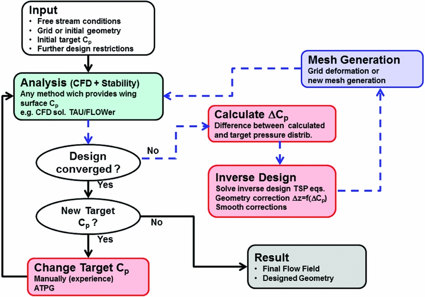
Figure 1. Inverse design process flowchart for application cases. Inner loop (dashed lines) is the inverse design process for a given target pressure distribution. In the outer loop (solid lines), the target pressure distribution is varied.
3.0 INVERSE DESIGN METHOD, GOVERNING EQUATIONS AND SOLUTION METHOD
In this section, the governing equations and numerical solution method of the inverse design method are described. Only cases for transonic free-stream Mach number with M∞<1 are considered. In the inverse design problem the unknown quantity is the wing surface geometry correction
 $\Delta {\bar{z}_ \pm }(\bar{x},\bar{y})$
, i.e. the difference between target wing geometry and actual wing geometry. Input or known quantity is the pressure distribution difference
$\Delta {\bar{z}_ \pm }(\bar{x},\bar{y})$
, i.e. the difference between target wing geometry and actual wing geometry. Input or known quantity is the pressure distribution difference
 $\Delta {C_{p \pm }}(\bar{x},\bar{y})$
between the target pressure distribution and computed pressure distribution of the actual geometry. Here ± denotes upper or lower wing surface. Let Φactual geometry
be the small perturbation velocity potential for the actual geometry and Φtarget
be the small perturbation velocity potential for the unknown geometry which leads to the desired target pressure distribution. In the inverse design method proposed by Takanashi(Reference Takanashi4), the TSP-equation is derived for the increment of the perturbation velocity potential ΔΦ, with ΔΦ = Φtarget
− Φ
actual geometry. It is given by:
$\Delta {C_{p \pm }}(\bar{x},\bar{y})$
between the target pressure distribution and computed pressure distribution of the actual geometry. Here ± denotes upper or lower wing surface. Let Φactual geometry
be the small perturbation velocity potential for the actual geometry and Φtarget
be the small perturbation velocity potential for the unknown geometry which leads to the desired target pressure distribution. In the inverse design method proposed by Takanashi(Reference Takanashi4), the TSP-equation is derived for the increment of the perturbation velocity potential ΔΦ, with ΔΦ = Φtarget
− Φ
actual geometry. It is given by:
 $$\begin{equation}
\Delta {\bar{\Phi }_{\bar{x}\bar{x}}} + \Delta {\bar{\Phi }_{\bar{y}\bar{y}}} + \Delta {\bar{\Phi }_{\bar{z}\bar{z}}} = \frac{\partial }{{\partial \bar{x}}}\underbrace {\left(\frac{1}{2}{{({{\bar{\Phi }}_{\bar{x}}} + \Delta {{\bar{\Phi }}_{\bar{x}}})}^2} - \frac{1}{2}{{({{\bar{\Phi }}_{\bar{x}}})}^2}\right)}_{\chi (\bar{x},\bar{y},\bar{z})}
\end{equation}$$
$$\begin{equation}
\Delta {\bar{\Phi }_{\bar{x}\bar{x}}} + \Delta {\bar{\Phi }_{\bar{y}\bar{y}}} + \Delta {\bar{\Phi }_{\bar{z}\bar{z}}} = \frac{\partial }{{\partial \bar{x}}}\underbrace {\left(\frac{1}{2}{{({{\bar{\Phi }}_{\bar{x}}} + \Delta {{\bar{\Phi }}_{\bar{x}}})}^2} - \frac{1}{2}{{({{\bar{\Phi }}_{\bar{x}}})}^2}\right)}_{\chi (\bar{x},\bar{y},\bar{z})}
\end{equation}$$
Here instead of the small perturbation potential Φ and the coordinate x, y, z the transformed quantities
 $\bar{\Phi }$
,
$\bar{\Phi }$
,
 $\bar{x},\bar{y},\bar{z}$
are used. They are obtained using a Prandtl-Glauert transformation:
$\bar{x},\bar{y},\bar{z}$
are used. They are obtained using a Prandtl-Glauert transformation:
 $$\begin{equation}
{\bar{x} = x}\;\, {\bar{y} = \beta y}\,\; {\bar{z} = \beta z}
\end{equation}$$
$$\begin{equation}
{\bar{x} = x}\;\, {\bar{y} = \beta y}\,\; {\bar{z} = \beta z}
\end{equation}$$
 $$\begin{equation}
\bar{\Phi }(\bar{x},\bar{y},\bar{z}) = \frac{K}{{{\beta ^2}}}\Phi (x,y,z).
\end{equation}$$
$$\begin{equation}
\bar{\Phi }(\bar{x},\bar{y},\bar{z}) = \frac{K}{{{\beta ^2}}}\Phi (x,y,z).
\end{equation}$$
Note that Equation (1) is an inhomogeneous Laplace equation. The function
 $\chi (\bar{x},\bar{y},\bar{z})$
(which is the inhomogeneous part of Equation (1)) will be considered in the following as a source term function. The quantities
$\chi (\bar{x},\bar{y},\bar{z})$
(which is the inhomogeneous part of Equation (1)) will be considered in the following as a source term function. The quantities
 $\Delta {\bar{z}_ \pm }(\bar{x},\bar{y})$
and
$\Delta {\bar{z}_ \pm }(\bar{x},\bar{y})$
and
 $\Delta {C_{p \pm }}(\bar{x},\bar{y})$
are related to partial derivatives of
$\Delta {C_{p \pm }}(\bar{x},\bar{y})$
are related to partial derivatives of
 $\bar{\Phi }$
, evaluated at the wing surface. The partial derivative of
$\bar{\Phi }$
, evaluated at the wing surface. The partial derivative of
 $\Delta {\bar{\Phi }_{\bar{z}}}$
is related with the wing surface geometry difference
$\Delta {\bar{\Phi }_{\bar{z}}}$
is related with the wing surface geometry difference
 $\Delta {\bar{z}_ \pm }(\bar{x},\bar{y})$
and the partial derivative of
$\Delta {\bar{z}_ \pm }(\bar{x},\bar{y})$
and the partial derivative of
 $\Delta {\bar{\Phi }_{\bar{x}}}$
is related with
$\Delta {\bar{\Phi }_{\bar{x}}}$
is related with
 $\Delta {C_{p \pm }}(\bar{x},\bar{y})$
according to:
$\Delta {C_{p \pm }}(\bar{x},\bar{y})$
according to:
 $$\begin{equation}
\Delta {\bar{\Phi }_{\bar{z}}}(\bar{x},\bar{y}, \pm 0) = \frac{K}{{{\beta ^3}}}\frac{{\partial \Delta {{\bar{z}}_ \pm }(\bar{x},\bar{y})}}{{\partial \bar{x}}}
\end{equation}$$
$$\begin{equation}
\Delta {\bar{\Phi }_{\bar{z}}}(\bar{x},\bar{y}, \pm 0) = \frac{K}{{{\beta ^3}}}\frac{{\partial \Delta {{\bar{z}}_ \pm }(\bar{x},\bar{y})}}{{\partial \bar{x}}}
\end{equation}$$
 $$\begin{equation}
\Delta {\bar{\Phi }_{\bar{x}}}(\bar{x},\bar{y}, \pm 0) = - \frac{K}{{2{\beta ^2}}}\Delta {C_{p \pm }}(\bar{x},\bar{y}).
\end{equation}$$
$$\begin{equation}
\Delta {\bar{\Phi }_{\bar{x}}}(\bar{x},\bar{y}, \pm 0) = - \frac{K}{{2{\beta ^2}}}\Delta {C_{p \pm }}(\bar{x},\bar{y}).
\end{equation}$$
K and ß are constants which depend on M∞:
 $$\begin{equation}
\begin{array}{*{20}{c}} {K = (\gamma + 1) \cdot M_\infty ^2,}&{\beta = \sqrt {1 - M_\infty ^2} } \end{array}
\end{equation}$$
$$\begin{equation}
\begin{array}{*{20}{c}} {K = (\gamma + 1) \cdot M_\infty ^2,}&{\beta = \sqrt {1 - M_\infty ^2} } \end{array}
\end{equation}$$
Using Green identities and several transformations, Takanashi(Reference Takanashi4) transformed the TSP-equation into integro-differential equations which relate the unknown
 $\Delta {\bar{\Phi }_{\bar{z}}}$
and the input
$\Delta {\bar{\Phi }_{\bar{z}}}$
and the input
 $\Delta {\bar{\Phi }_{\bar{x}}}$
. These transformations are not given here and the reader can find them in Reference TakanashiRefs 4 and Reference Bartelheimer5. For the transformations, it was convenient to introduce new quantities defined as symmetrical and asymmetrical transformations of
$\Delta {\bar{\Phi }_{\bar{x}}}$
. These transformations are not given here and the reader can find them in Reference TakanashiRefs 4 and Reference Bartelheimer5. For the transformations, it was convenient to introduce new quantities defined as symmetrical and asymmetrical transformations of
 $\Delta {\bar{\Phi }_{\bar{x}}}$
,
$\Delta {\bar{\Phi }_{\bar{x}}}$
,
 $\Delta {\bar{\Phi }_{\bar{z}}}$
and the source term χ with respect to the upper and lower wing surface side:
$\Delta {\bar{\Phi }_{\bar{z}}}$
and the source term χ with respect to the upper and lower wing surface side:
 $$\begin{equation}
\begin{array}{@{}*{1}{c}@{}} {\Delta {u_s}(\bar{x},\bar{y}) = \Delta {{\bar{\Phi }}_{\bar{x}}}(\bar{x},\bar{y}, + 0) + \Delta {{\bar{\Phi }}_{\bar{x}}}(\bar{x},\bar{y}, - 0)}\\ {\Delta {w_s}(\bar{x},\bar{y}) = \Delta {{\bar{\Phi }}_{\bar{z}}}(\bar{x},\bar{y}, + 0) - \Delta {{\bar{\Phi }}_{\bar{z}}}(\bar{x},\bar{y}, - 0)}\\ {{\chi _s}(\bar{x},\bar{y}) = \chi (\bar{x},\bar{y}, + 0) + \chi (\bar{x},\bar{y}, - 0)} \end{array}
\end{equation}$$
$$\begin{equation}
\begin{array}{@{}*{1}{c}@{}} {\Delta {u_s}(\bar{x},\bar{y}) = \Delta {{\bar{\Phi }}_{\bar{x}}}(\bar{x},\bar{y}, + 0) + \Delta {{\bar{\Phi }}_{\bar{x}}}(\bar{x},\bar{y}, - 0)}\\ {\Delta {w_s}(\bar{x},\bar{y}) = \Delta {{\bar{\Phi }}_{\bar{z}}}(\bar{x},\bar{y}, + 0) - \Delta {{\bar{\Phi }}_{\bar{z}}}(\bar{x},\bar{y}, - 0)}\\ {{\chi _s}(\bar{x},\bar{y}) = \chi (\bar{x},\bar{y}, + 0) + \chi (\bar{x},\bar{y}, - 0)} \end{array}
\end{equation}$$
 $$\begin{equation}
\begin{array}{@{}*{1}{c}@{}} {\Delta {u_a}(\bar{x},\bar{y}) = \Delta {{\bar{\Phi }}_{\bar{x}}}(\bar{x},\bar{y}, + 0) - \Delta {{\bar{\Phi }}_{\bar{x}}}(\bar{x},\bar{y}, - 0)}\\ {\Delta {w_a}(\bar{x},\bar{y}) = \Delta {{\bar{\Phi }}_{\bar{z}}}(\bar{x},\bar{y}, + 0) + \Delta {{\bar{\Phi }}_{\bar{z}}}(\bar{x},\bar{y}, - 0)} \end{array}
\end{equation}$$
$$\begin{equation}
\begin{array}{@{}*{1}{c}@{}} {\Delta {u_a}(\bar{x},\bar{y}) = \Delta {{\bar{\Phi }}_{\bar{x}}}(\bar{x},\bar{y}, + 0) - \Delta {{\bar{\Phi }}_{\bar{x}}}(\bar{x},\bar{y}, - 0)}\\ {\Delta {w_a}(\bar{x},\bar{y}) = \Delta {{\bar{\Phi }}_{\bar{z}}}(\bar{x},\bar{y}, + 0) + \Delta {{\bar{\Phi }}_{\bar{z}}}(\bar{x},\bar{y}, - 0)} \end{array}
\end{equation}$$
Note that different signs have been used in (7) and (8) for Δus and Δws , and Δua and Δwa . This is because a symmetrical/asymmetrical pressure distribution change leads to an asymmetrical/symmetrical change in the geometry correction. For the numerical solution, the integro-differential equations are discretised(Reference Takanashi4,Reference Bartelheimer5) . A panel mesh with I x (J + 1) panels is constructed for the wing surface. For the definition of indices and points on the panel mesh, see Fig. 2, which shows a panel mesh for a half wing. In the discretisation process, it is assumed that the quantities Δwa , Δus , Δua , χ and χ s are constant for each panel. For panel (i, j), they are evaluated at the panel centre coordinate (xj i , yj ).

Figure 2. Discretised wing for inverse design method. The wing surface is discretised in I × (J+1) panels. with I = 7 and J = 7. Figure is based on Fig. 4 from Reference BartelheimerRef. 5.
For the quantity Δws
, it is assumed that for each panel this quantity varies linearly along the
 $\bar{x}$
-direction, but is constant along the
$\bar{x}$
-direction, but is constant along the
 $\bar{y}$
-direction. Therefore, for a panel row with constant span
$\bar{y}$
-direction. Therefore, for a panel row with constant span
 ${\bar{y}_j} = {\rm{const}}.$
, Δws
is discretised in
${\bar{y}_j} = {\rm{const}}.$
, Δws
is discretised in
 $\bar{x}$
-direction at coordinates xj
i − 1/2
, yj
with 1 < i < I + 1. Note that this discretisation leads to I+1 unknown for I given known quantities. In order to have a unique solution Takanashi(Reference Takanashi4) proposed an additional condition for Δws
which leads to closed aerofoils, provided the initial aerofoil is closed. In discretised form, this condition requires that for each section:
$\bar{x}$
-direction at coordinates xj
i − 1/2
, yj
with 1 < i < I + 1. Note that this discretisation leads to I+1 unknown for I given known quantities. In order to have a unique solution Takanashi(Reference Takanashi4) proposed an additional condition for Δws
which leads to closed aerofoils, provided the initial aerofoil is closed. In discretised form, this condition requires that for each section:
 $$\begin{equation}
\sum\nolimits_{i = 1}^I {0.5\;\Big[\Delta {w_s}\Big(x} _{i - ^1{\!\!/\!}_{2}}^j,{y_j}\Big) + \Delta {w_s}\Big(x_{i + ^1{\!\!/\!}_{2}}^j,{y_j}\Big)\Big]\Big(x_{i + ^1{\!\!/\!}_{2}}^j - x_{i - ^1{\!\!/\!}_{2}}^j\Big) = 0
\end{equation}$$
$$\begin{equation}
\sum\nolimits_{i = 1}^I {0.5\;\Big[\Delta {w_s}\Big(x} _{i - ^1{\!\!/\!}_{2}}^j,{y_j}\Big) + \Delta {w_s}\Big(x_{i + ^1{\!\!/\!}_{2}}^j,{y_j}\Big)\Big]\Big(x_{i + ^1{\!\!/\!}_{2}}^j - x_{i - ^1{\!\!/\!}_{2}}^j\Big) = 0
\end{equation}$$
Physically, this additional condition means that the trailing-edge thickness for each section of the designed wing is the same as the trailing-edge thickness of the initial wing.
The discretised equations for the inverse problem for the case of a wing with symmetrical flow are given by Reference TakanashiRefs 4 and Reference Bartelheimer5.
 $$\begin{eqnarray}
&&{\Delta {u_s}\left(\bar{x}_i^j,{{\bar{y}}_j}\right) = \sum\limits_{i = 1}^{I + 1} {\sum\limits_{m = 0}^J {\left[\mu _{i,j,l,m}^s\Delta {w_s}\left(\bar{x}_{l - 1/2}^m,{{\bar{y}}_m}\right)\right] + {\chi _s}\left(\bar{x}_i^j,{{\bar{y}}_j}\right)} } }\nonumber\\
&&\quad+\, \sum\limits_{i = 1}^I \sum\limits_{m = 0}^J \left[\,\nu _{i,j,l,m}^s\chi \left(\bar{x}_l^m,{{\bar{y}}_m}, + 0\right) + \,\nu _{i,j,l,m}^{*s}\chi \left(\bar{x}_l^m,{{\bar{y}}_m}, - 0\right)\right]
\end{eqnarray}$$
$$\begin{eqnarray}
&&{\Delta {u_s}\left(\bar{x}_i^j,{{\bar{y}}_j}\right) = \sum\limits_{i = 1}^{I + 1} {\sum\limits_{m = 0}^J {\left[\mu _{i,j,l,m}^s\Delta {w_s}\left(\bar{x}_{l - 1/2}^m,{{\bar{y}}_m}\right)\right] + {\chi _s}\left(\bar{x}_i^j,{{\bar{y}}_j}\right)} } }\nonumber\\
&&\quad+\, \sum\limits_{i = 1}^I \sum\limits_{m = 0}^J \left[\,\nu _{i,j,l,m}^s\chi \left(\bar{x}_l^m,{{\bar{y}}_m}, + 0\right) + \,\nu _{i,j,l,m}^{*s}\chi \left(\bar{x}_l^m,{{\bar{y}}_m}, - 0\right)\right]
\end{eqnarray}$$
 $$\begin{eqnarray}
&&{\Delta {w_a}(\bar{x}_i^j,{{\bar{y}}_j}) = \sum\limits_{i = 1}^I {\sum\limits_{m = 0}^J {\left[\mu _{i,j,l,m}^a\Delta {u_a}\left(\bar{x}_l^m,{{\bar{y}}_m}\right)\right] } } }\nonumber\\
&&\quad+\, \sum\limits_{i = 1}^I \sum\limits_{m = 0}^J \left[\nu _{i,j,l,m}^a\chi \left(\bar{x}_l^m,{{\bar{y}}_m}, + 0\right) + \nu _{i,j,l,m}^{*a}\chi \left(\bar{x}_l^m,{{\bar{y}}_m}, - 0\right)\right]
\end{eqnarray}$$
$$\begin{eqnarray}
&&{\Delta {w_a}(\bar{x}_i^j,{{\bar{y}}_j}) = \sum\limits_{i = 1}^I {\sum\limits_{m = 0}^J {\left[\mu _{i,j,l,m}^a\Delta {u_a}\left(\bar{x}_l^m,{{\bar{y}}_m}\right)\right] } } }\nonumber\\
&&\quad+\, \sum\limits_{i = 1}^I \sum\limits_{m = 0}^J \left[\nu _{i,j,l,m}^a\chi \left(\bar{x}_l^m,{{\bar{y}}_m}, + 0\right) + \nu _{i,j,l,m}^{*a}\chi \left(\bar{x}_l^m,{{\bar{y}}_m}, - 0\right)\right]
\end{eqnarray}$$
In these equations, μ s i, j, l, m , μ i, j, l, m a , ν s i, j, l, m , ν i, j, l, m * s , ν a i, j, l, m , ν i, j, l, m * a are influence coefficients. Equations (10) and (11) are two linear equation systems. For the computation of the quantities Δwa and Δus for panel (i, j), the influence of all panels (l, m) of the wing have to be taken into account, including panels on the not shown other wing half (see Fig. 2). For a symmetrical flow for a given panel (l, m) and its corresponding symmetrical panel (l, −m) the quantities Δws , Δwa , Δus , Δua , χ and χ s are equal. When they appear on the right side of Equations (10) and (11), they will be denoted as source terms. For a symmetrical case, the sum in Equations (10) and (11) can be restricted to one half-wing if the influence coefficient with index i, j, l, m includes both, the contribution from panel (l, m) and the contribution from the corresponding symmetrical wing panel with index (l, −m). The influence coefficients are integrals over panel (l, m) and its corresponding symmetrical panel (l, −m). For influence coefficients μ s i, j, l, m , μ i, j, l, m a , these integrals involve surface integrals over the panel surface, whereas for ν s i, j, l, m , ν i, j, l, m * s , ν a i, j, l, m , ν i, j, l, m * a field integrals are required, i.e. additional integration in direction normal to the panel surface is required. They are not solved numerically but, as first proposed by Hua and Zhang(Reference Hua and Zhang25), they can be solved analytically. This simplifies the numerical solution method. The analytical expressions for the influence coefficients are given in Reference BartelheimerRef. 5. Note that the asymmetrical geometry corrections Δwa are explicitly given by Equation (11), whereas to obtain the symmetrical geometry corrections Δws the linear system of equations given in Equation (10) has to be inverted. Finally, the obtained Δwa and Δws are used to obtain the geometry correction according to:
 $$\begin{equation}
\Delta {\bar{z}_ \pm }(\bar{x},\bar{y}) = \frac{{{\beta ^3}}}{{2K}}\int\limits_{{{\bar{x}}_{LE}}}^{\bar{x}} {(\Delta {w_a}} (\bar{x},\bar{y}) \pm \Delta {w_s}(\bar{x},\bar{y}))d\bar{x}
\end{equation}$$
$$\begin{equation}
\Delta {\bar{z}_ \pm }(\bar{x},\bar{y}) = \frac{{{\beta ^3}}}{{2K}}\int\limits_{{{\bar{x}}_{LE}}}^{\bar{x}} {(\Delta {w_a}} (\bar{x},\bar{y}) \pm \Delta {w_s}(\bar{x},\bar{y}))d\bar{x}
\end{equation}$$
4.0 MODIFICATIONS FOR FLOW WITH HIGH TRANSONIC MACH NUMBER
For transonic flow, Bartelheimer(Reference Barthelheimer6) introduced two modifications into the solution scheme which improved the convergence of the design especially for regions in which the local flow is supersonic. The first modification altered the governing equation for regions were the flow is supersonic. The second introduced modification is smoothing of the geometry.
The solution algorithm of the governing equation (Equation (1)) does not distinguish between an elliptic (subsonic) or a hyperbolic (supersonic) character of Equation (1). The character of the governing equation (Equation (1)) is elliptic or hyperbolic if:
 $$\begin{equation}
\begin{array}{@{}l@{}} (1 - {{\bar{\Phi }}_{\bar{x}}} - \Delta {{\bar{\Phi }}_{\bar{x}}})\; > \;0\; {\rm{elliptic}}\\ (1 - {{\bar{\Phi }}_{\bar{x}}} - \Delta {{\bar{\Phi }}_{\bar{x}}})\; < 0\;{\rm{hyperbolic}}{\rm{.}} \end{array}
\end{equation}$$
$$\begin{equation}
\begin{array}{@{}l@{}} (1 - {{\bar{\Phi }}_{\bar{x}}} - \Delta {{\bar{\Phi }}_{\bar{x}}})\; > \;0\; {\rm{elliptic}}\\ (1 - {{\bar{\Phi }}_{\bar{x}}} - \Delta {{\bar{\Phi }}_{\bar{x}}})\; < 0\;{\rm{hyperbolic}}{\rm{.}} \end{array}
\end{equation}$$
The integro-differential equation for the inverse design is obtained by using Green functions for the Laplace equation, which has elliptic character. In order to extend the solution regions also to hyperbolic regions an upwind discretisation scheme is used (see Reference BarthelheimerRef. 6). If the upwind discretisation of Equation (1) is written with central discretisation a modified governing equation results:
 $$\begin{equation}
\Delta {\bar{\Phi }_{\bar{x}\bar{x}}} + \Delta {\bar{\Phi }_{\bar{y}\bar{y}}} + \Delta {\bar{\Phi }_{\bar{z}\bar{z}}} = \frac{\partial }{{\partial \bar{x}}}\underbrace {\left[\frac{1}{2}{{({{\bar{\Phi }}_{\bar{x}}} + \Delta {{\bar{\Phi }}_{\bar{x}}})}^2} - \frac{1}{2}{{({{\bar{\Phi }}_{\bar{x}}})}^2} + \Delta \bar{x}\Delta {{\bar{\Phi }}_{\bar{x}\bar{x}}}(1 - {{\bar{\Phi }}_{\bar{x}}} - \Delta {{\bar{\Phi }}_{\bar{x}}})\right]}_{{\chi ^*}(\bar{x},\bar{y},\bar{z})}
\end{equation}$$
$$\begin{equation}
\Delta {\bar{\Phi }_{\bar{x}\bar{x}}} + \Delta {\bar{\Phi }_{\bar{y}\bar{y}}} + \Delta {\bar{\Phi }_{\bar{z}\bar{z}}} = \frac{\partial }{{\partial \bar{x}}}\underbrace {\left[\frac{1}{2}{{({{\bar{\Phi }}_{\bar{x}}} + \Delta {{\bar{\Phi }}_{\bar{x}}})}^2} - \frac{1}{2}{{({{\bar{\Phi }}_{\bar{x}}})}^2} + \Delta \bar{x}\Delta {{\bar{\Phi }}_{\bar{x}\bar{x}}}(1 - {{\bar{\Phi }}_{\bar{x}}} - \Delta {{\bar{\Phi }}_{\bar{x}}})\right]}_{{\chi ^*}(\bar{x},\bar{y},\bar{z})}
\end{equation}$$
Note that Equation (14) is the same as Equation (1) with a modified right-hand side. Therefore, the solution method for hyperbolic regions is the same but using the modified function χ* instead of χ. This modification stabilised the convergence of the design for transonic flow.
The second modification introduced in Reference BarthelheimerRef. 6 is smoothing of the geometry correction. Since the computed pressure distribution is obtained with a CFD solution, it is provided with a certain small amount of numerical error. This numerical error is included in the input pressure distribution difference ΔCp for the inverse design. The inverse design method may not be able to damp this error. To avoid small oscillations in the designed geometry due to numerical error transfer between two coupled numerical methods, smoothing of the geometry correction is introduced in the design solution process. For transonic flow, this is even more important since small geometry differences lead to large ΔCp ’s.
With these modifications, the inverse design method could be improved significantly for transonic flow cases. However, in some test cases with high transonic Mach number, i.e. for Mach numbers with 0.85 < M ∞ < 1.00, it was not possible to obtain a converged design, even if the previously mentioned modifications are used. For these cases, a relaxed geometry change was used already in order to improve design stability. A relaxed geometry change is one in which in each design iteration, the symmetrical and asymmetrical geometry change is reduced by multiplying with factors rfs, respectively rfa (with 0 < rfa < 1, 0 < rfs < 1.
In this work, further modifications of the solution scheme were introduced in regions were the governing equation has hypersonic character. Several modifications were tested with the aim to take into account the upwind character of the solution. The following modification improved the stability of the design process. First, the determination of the elliptical or hyperbolical character according to Equation (13) was obtained with an upwind discretisation of the partial derivatives. Second, additional supersonic influence terms g i, j and h i, j, l, m are introduced in the linear equation system Equations (10) and (11). These terms introduce for the source terms χ a region of influence within supersonic regions. Their value is either one or zero by taking into account if at panel (i, j) or/and panel (l, m) the flow is supersonic.
 $$\begin{eqnarray}
&&\Delta {u_s}(\bar{x}_i^j,{{\bar{y}}_j}) = \sum\limits_{i = 1}^{I + 1} \sum\limits_{m = 0}^J [\mu _{i,j,l,m}^s\Delta {w_s}(\bar{x}_{l - 1/2}^m,{{\bar{y}}_m})] + {g_{i,j}}( + 0)\chi (\bar{x}_i^j,{{\bar{y}}_j}, + 0)\nonumber\\
&&\qquad\qquad\qquad + {g_{i,j}}( - 0)\chi (\bar{x}_i^j,{{\bar{y}}_j}, - 0) \nonumber\\
&&\quad + \sum\limits_{i = 1}^I \sum\limits_{m = 0}^J {[{h_{i,j,l,m}}( + 0)\nu _{i,j,l,m}^s\chi (\bar{x}_l^m,{{\bar{y}}_m}, + 0) + {h_{i,j,l,m}}( - 0)\nu _{i,j,l,m}^{*s}\chi (\bar{x}_l^m,{{\bar{y}}_m}, - 0)]}\nonumber\\
\end{eqnarray}$$
$$\begin{eqnarray}
&&\Delta {u_s}(\bar{x}_i^j,{{\bar{y}}_j}) = \sum\limits_{i = 1}^{I + 1} \sum\limits_{m = 0}^J [\mu _{i,j,l,m}^s\Delta {w_s}(\bar{x}_{l - 1/2}^m,{{\bar{y}}_m})] + {g_{i,j}}( + 0)\chi (\bar{x}_i^j,{{\bar{y}}_j}, + 0)\nonumber\\
&&\qquad\qquad\qquad + {g_{i,j}}( - 0)\chi (\bar{x}_i^j,{{\bar{y}}_j}, - 0) \nonumber\\
&&\quad + \sum\limits_{i = 1}^I \sum\limits_{m = 0}^J {[{h_{i,j,l,m}}( + 0)\nu _{i,j,l,m}^s\chi (\bar{x}_l^m,{{\bar{y}}_m}, + 0) + {h_{i,j,l,m}}( - 0)\nu _{i,j,l,m}^{*s}\chi (\bar{x}_l^m,{{\bar{y}}_m}, - 0)]}\nonumber\\
\end{eqnarray}$$
 $$\begin{eqnarray}
&&\Delta {w_a}(\bar{x}_i^j,{{\bar{y}}_j}) = \sum\limits_{i = 1}^I \sum\limits_{m = 0}^J [\mu _{i,j,l,m}^a\Delta {u_a}(\bar{x}_l^m,{{\bar{y}}_m})]\nonumber \\
&&\quad +\sum\limits_{i = 1}^I \sum\limits_{m = 0}^J [{h_{i,j,l,m}}( + 0)\nu _{i,j,l,m}^a\chi (\bar{x}_l^m,{{\bar{y}}_m}, + 0) + {h_{i,j,l,m}}( - 0)\nu _{i,j,l,m}^{*a}\chi (\bar{x}_l^m,{{\bar{y}}_m}, - 0)]\nonumber\\
\end{eqnarray}$$
$$\begin{eqnarray}
&&\Delta {w_a}(\bar{x}_i^j,{{\bar{y}}_j}) = \sum\limits_{i = 1}^I \sum\limits_{m = 0}^J [\mu _{i,j,l,m}^a\Delta {u_a}(\bar{x}_l^m,{{\bar{y}}_m})]\nonumber \\
&&\quad +\sum\limits_{i = 1}^I \sum\limits_{m = 0}^J [{h_{i,j,l,m}}( + 0)\nu _{i,j,l,m}^a\chi (\bar{x}_l^m,{{\bar{y}}_m}, + 0) + {h_{i,j,l,m}}( - 0)\nu _{i,j,l,m}^{*a}\chi (\bar{x}_l^m,{{\bar{y}}_m}, - 0)]\nonumber\\
\end{eqnarray}$$
By testing different choices for the supersonic influence terms, it was found that following simple selection of supersonic influence terms g i, j and h i, j, l, m stabilises the iterative design for high transonic numbers: h i, j, l, m = 0 if the flow is supersonic for panel (i, j) and simultaneously for panel (l, m) it is satisfied that the flow is supersonic and xi > xl , otherwise, h i, j, l, m = 1, g i, j = 0; if the flow is supersonic at panel (i, j), otherwise g i, j = 1. These selections were obtained by first testing design cases in which only the solution of Equation (15) is required. Such design cases are obtained if the design of symmetrical aerofoils is considered for a constant angle-of-attack. Then, design cases were tested which require the solution of both Equations (15) and (16).
Finally, a comment is given, regarding the here-described extension for high-transonic Mach numbers of the original Takanashi transonic inverse design method in comparison to Matsushima's inverse design method for supersonic flow(Reference Matsushima and Takanashi10,Reference Matsushima, Iwamiya and Nakahashi12) . The approaches taken to consider supersonic flow (or regions of supersonic flow in a transonic flow) are different. Here we consider transonic free-stream Mach numbers very close to 1 but with M ∞<1. Therefore, the integro-differential TSP equations for the transonic flow considered here are derived using elliptical Green functions. They are obtained following the original approach given by Takanashi(Reference Takanashi4). In contrast, if the free-stream number is supersonic, hyperbolic Green functions are required in order to obtain the integro-differential equations. For the supersonic case, this is done by Matsushima(Reference Matsushima and Takanashi10) for the linearised small perturbation velocity equation. For the case with transonic free-stream Mach number considered here, the character of the complete non-linear TSP equation is hyperbolic or elliptic according to Equation (13). In regions where the local flow becomes supersonic (or the equation character hyperbolic), the above-described modified non-linear source term χ* is used. The original DLR inverse design method(Reference Bartelheimer5) already used a modified source term, which was further modified in this work. The results presented in the next section show that the use of the further modified source term has improved the convergence of the design solutions for cases with mixed character, i.e. subsonic and supersonic flow regions. Especially, for transonic free-stream Mach numbers close to 1 converged design solutions are obtained for cases where the original DLR inverse design method failed.
4.1 Results for redesign test cases
Results for the modified method considering 2D aerofoil and 3D wing redesign cases are described. The first case is a symmetrical aerofoil redesign test case in which only Equation (15) is tested. Free-stream conditions are: M ∞ = 0.9 for α = 0°. Initial geometry is a NACA aerofoil with 1.2% thickness and the target pressure distribution is obtained for a NACA0006 aerofoil for M ∞ = 0.9, Rec = 30 · 106 for α = 0°. Due to the high free-stream Mach number, very thin aerofoils have been selected. The initial aerofoil is sufficiently thin so that with the specified free-stream conditions the pressure distribution of the initial aerofoil is completely subsonic. In contrast, the target aerofoil pressure distribution has a large supersonic region but with Mach numbers not exceeding M = 1.3. Figure 3 shows the initial, target and designed pressure distribution and aerofoil geometry. Figure 4 shows the convergence of the mean square pressure distribution change and the mean square geometry deviation for design iterations. Thirty design iterations were performed. The original method does not converge to the target design pressure distribution, even after decreasing the factor rfs to the value rfs = 0.1. After 13 design iterations, the mean square change of pressure distribution between design iterations increases. For the modified method, the design converges to the prescribed target even with a four times larger geometry change between design iterations (rfs = 0.4). The second case considered is a 2D aerofoil redesign case in which both Equations (15) and (16) are tested. Here a NACA0006 geometry is designed into an aerofoil based on a modified middle-wing section of the DLR F-11 wing(Reference Wichmann, Strohmeyer and Streit26). Free-stream Mach number is 0.9. Since the DLR F-11 model has a swept wing and is designed for M ∞ = 0.85, the aerofoil thickness of the selected modified DLR-F11 target section is reduced. The initial solution is obtained for M ∞ = 0.9, α = 0°, Rec = 30 · 106. The target pressure distribution is obtained for M ∞ = 0.9, α = 0.5°, Rec = 30 · 106. Figures 5 and 6 shows the comparison between the redesign results for the original method and the new method. As in the previous case the original method is not able to produce a converged design result even with a small value for the geometry relaxation parameter rfa and rfs. The designed pressure distribution oscillates around the target pressure distribution and after 13 design iterations the mean square changes in pressure distribution begin to increase. The modified method design result reproduces the target pressure distribution and geometry. The new method converges with a 4 times larger value for the geometry relaxation parameters rfa and rfs.

Figure 3. Redesign case for symmetrical aerofoils for M ∞ = 0.9, Rec = 30 · 106, α = 0°. Results are given for the pressure distribution (left) and geometry (right) for the initial, target and design solutions. Design results are obtained with original and new modified inverse design method.
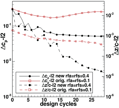
Figure 4. Convergence history for redesign case considered in Fig. 3.

Figure 5. Second aerofoil redesign case for M ∞ = 0.9, Rec = 30 · 106. Initial geometry and target pressure distribution for NACA0006 for α = 0°. Results are given for the pressure distribution (left) and geometry (right) for the initial, target and design solutions. Design results are obtained with original and modified inverse design method.
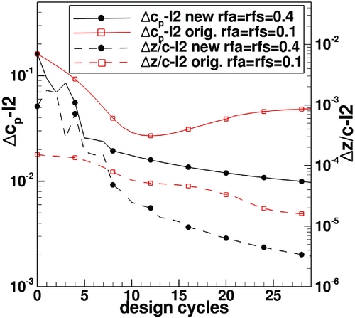
Figure 6. Convergence history for redesign case considered in Fig. 5.
The third redesign case considered is a 3D-case. For this case a constant chord swept wing with untwisted constant aerofoil sections was selected. The sweep of the wing is 30°, chord to semispan ratio is c/s = 0.2, free-stream conditions are M ∞ = 0.95, Rec = 13 · 106. For the target geometry, a swept wing geometry, the modified DLR-F11 middle wing section with a reduced thickness is used and the target pressure distribution was obtained for a lift value cL = 0.5. For the initial swept-wing geometry, a NACA0006 aerofoil is used and the starting solution for the design was computed at α = 0°. For the design iterations, the geometry relaxation parameters were used with values rfa = rfs = 0.2. Similarly, as in the previous 2D cases, with the original inverse design method it was not possible to obtain a converged design. Results for the modified method are shown for selected wing sections in Fig. 7. Except for small suction peaks at the nose, the designed results match the target pressure distribution. This shows that the introduced modifications are able to improve the inverse design method for the 3D case.

Figure 7. 3D redesign case for M ∞ = 0.95, Rec = 13 · 106, 30° swept wing. Results are given for geometry (left) and the pressure distribution (right) for the initial (dashed line), target (squares) and design solutions (solid line). Wing planform is shown in the middle with lines indicating the position of the selected sections. Design results are obtained with the new modified inverse design method.
5.0 EXTENSION OF THE INVERSE CODE TO NON-PLANAR CONFIGURATIONS
The second modification is the extension of the inverse design program to non-planar wings. Since geometry deformations are in the z-direction the original design code is restricted to non-planar wing designs with small dihedral. The solution method of the TSP-equations was modified in such a way that now geometry corrections are provided locally in a direction perpendicular to the local wing surface. This extends the applicability to non-planar wings with large dihedral for example wings with large vertical wings, or non-conventional wing configurations like box wings, C-wings etc. Previously, the inverse design code had been modified for the design of nacelles, see Reference Hepperle, Bartelheimer and BousquetRefs 8 and Reference Wilhelm9. Nacelles can be considered as a ring wing with a circular trailing edge. Following the modifications introduced in Reference WilhelmRef. 9, here the inverse code is generalised to arbitrary non-planar wings. In the generalisation, it is assumed that there is a wing surface line in spanwise direction which remains fixed in the design process and which defines the non-planar front shape of the wing (see Fig. 8). To solve the corresponding TSP-equations here the YZ-projection of the trailing-edge line is selected as such a wing front line. Similarly, as shown in Fig. 1, a panel mesh is defined for the non-planar wing.
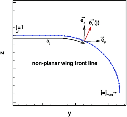
Figure 8. Front line of a non-planar wing with a planar inner part and a 1/4th ring wing in the outer part. The unit vectors
 ${\vec{e}_t},{\vec{e}_y}$
and
${\vec{e}_t},{\vec{e}_y}$
and
 ${\vec{e}_z}$
are shown for the point with index j. The arc-length sj
of the front line defines the spanwise coordinate of the non-planar wing.
${\vec{e}_z}$
are shown for the point with index j. The arc-length sj
of the front line defines the spanwise coordinate of the non-planar wing.
The front line is discretised in the span direction. For the discretised points on this line, aerofoil sections are defined in the corresponding plane perpendicular to the front line and discretised in streamwise direction. Also, the computed design deformations will be performed in these perpendicular planes. The coordinate perpendicular to the front line is denoted t, the span position coordinate is denoted s. In contrast to the planar case in which for a given point (i, j) the design span coordinate is defined by the distance y
i, j
to the symmetry plane, here the span position
 ${s_{\hbox{\scriptsize\itshape\'i},j}}$
is defined by the arc-length sj
of the corresponding trailing-edge point computed on the wing front line. Note that the so-selected curvilinear coordinate system (x, s, t) is the coordinate system of a planar wing which corresponds to the unrolled non-planar wing. The discretised TSP-equations (Equations (10) and (11)) for the non-planar wing, are obtained by replacing the panel surface Cartesian coordinates x
i, j
, y
i, j
, z
i, j
with the non-planar coordinates x
i, j
, s
i, j
, t
i, j
Finally, the computed design deformations Δt
n + 1
i, j
, computed in the curvilinear system for design iteration n+1 are computed in the Cartesian coordinate system using:
${s_{\hbox{\scriptsize\itshape\'i},j}}$
is defined by the arc-length sj
of the corresponding trailing-edge point computed on the wing front line. Note that the so-selected curvilinear coordinate system (x, s, t) is the coordinate system of a planar wing which corresponds to the unrolled non-planar wing. The discretised TSP-equations (Equations (10) and (11)) for the non-planar wing, are obtained by replacing the panel surface Cartesian coordinates x
i, j
, y
i, j
, z
i, j
with the non-planar coordinates x
i, j
, s
i, j
, t
i, j
Finally, the computed design deformations Δt
n + 1
i, j
, computed in the curvilinear system for design iteration n+1 are computed in the Cartesian coordinate system using:
 $$\begin{equation}
\begin{array}{@{}*{1}{c}@{}} {x_{i,j}^{n + 1} = x_{i,j}^n}\\[4pt] {y_{i,j}^{n + 1} = y_{i,j}^n + \Delta t_{i,j}^{n + 1}{{\vec{e}}_t}(j) \cdot {{\vec{e}}_y}}\\[4pt] {z_{i,j}^{n + 1} = z_{i,j}^n + \Delta t_{i,j}^{n + 1}{{\vec{e}}_t}(j) \cdot {{\vec{e}}_z}} \end{array}
\end{equation}$$
$$\begin{equation}
\begin{array}{@{}*{1}{c}@{}} {x_{i,j}^{n + 1} = x_{i,j}^n}\\[4pt] {y_{i,j}^{n + 1} = y_{i,j}^n + \Delta t_{i,j}^{n + 1}{{\vec{e}}_t}(j) \cdot {{\vec{e}}_y}}\\[4pt] {z_{i,j}^{n + 1} = z_{i,j}^n + \Delta t_{i,j}^{n + 1}{{\vec{e}}_t}(j) \cdot {{\vec{e}}_z}} \end{array}
\end{equation}$$
 ${\vec{e}_t}(j),\;{\vec{e}_y}$
and
${\vec{e}_t}(j),\;{\vec{e}_y}$
and
 ${\vec{e}_z}$
are unit vectors with
${\vec{e}_z}$
are unit vectors with
 ${\vec{e}_t}(j)$
the normal vector to the wing front line for point j and
${\vec{e}_t}(j)$
the normal vector to the wing front line for point j and
 ${\vec{e}_y},\;{\vec{e}_z}$
are unit vectors in the Cartesian directions y, z, see Fig. 8. In the original inverse design method, the wing planform, defined as the wing projection in the XY-plane is kept constant in the design. For the non-planar inverse design TSP method presented here, the constant planform is obtained by spanwise locally projecting the wing with the vector
${\vec{e}_y},\;{\vec{e}_z}$
are unit vectors in the Cartesian directions y, z, see Fig. 8. In the original inverse design method, the wing planform, defined as the wing projection in the XY-plane is kept constant in the design. For the non-planar inverse design TSP method presented here, the constant planform is obtained by spanwise locally projecting the wing with the vector
 ${\vec{e}_t}(j)$
. It was mentioned above that the front line was obtained using the YZ projection of the wing trailing edge. This means that in the design all local twist changes are performed around the trailing edge. If design requirements specify that aerofoils have to be twisted around a point lying at a different chord position xT
(j)/c(j), the computed geometry deformation with fixed trailing edge are shifted by redistributing them linearly as function of streamwise direction so that a zero deformation results for the point xT
(j)/c(j). After each design iteration, a shift of twist line transformation is performed. This guarantees a constant planform.
${\vec{e}_t}(j)$
. It was mentioned above that the front line was obtained using the YZ projection of the wing trailing edge. This means that in the design all local twist changes are performed around the trailing edge. If design requirements specify that aerofoils have to be twisted around a point lying at a different chord position xT
(j)/c(j), the computed geometry deformation with fixed trailing edge are shifted by redistributing them linearly as function of streamwise direction so that a zero deformation results for the point xT
(j)/c(j). After each design iteration, a shift of twist line transformation is performed. This guarantees a constant planform.
Next, results for the extended non-planar inverse design code are presented. As a test case, a constant unswept chord non-planar wing was selected. In the inner part of the wing, it has a planar planform, whereas the outer part has a 1/4th ring wing geometry (see insert in Fig. 9). The free-stream Mach number is M ∞ = 0.82. The initial wing geometry was constructed using a constant NACA0006 aerofoil twisted 2° down around the trailing edge (with twist direction in a plane perpendicular to the trailing edge). At the tip, the 2° twist difference was blended to 0°. The target pressure distribution is obtained using a wing geometry constructed with an untwisted modified DLR-F11-wing reduced-thickness aerofoil. Flow solutions were obtained for M ∞ = 0.82, Rec = 15 · 106, α = 4°. In Fig. 9 pressure distribution results for selected sections are given for initial, design and target pressure. Note that since the used wing has no sweep, the target pressure distributions have strong shocks. Therefore, it was necessary to use the inverse method with the modifications for transonic flow described before. Results are given for the design iteration 22. But results for iteration 15 show that the agreement between designed pressure distribution and target pressure distribution is good. But the convergence to the target geometry is slower than the convergence to the target pressure distribution. Especially in the tip region after 22 design iterations the target geometry and design geometry results still shows deviations. Also the twist has not reached the target twist. It oscillates around the target twist value, its absolute value differing at maximum by 0.2°. For geometry additional design iterations are required. This is shown in Fig. 10, where the initial geometry and the designed geometry are given for design iterations 22 and 33. Figure 11 shows the convergence history. As described above, the mean square pressure distribution deviations do not change largely after 16 iterations, while the mean square geometry deviations still decrease by an order of magnitude between 16 and 33 design iterations. The used value of the geometry relaxation parameter rfa and rfs is 0.5. Here the results were presented for a case in which the target wing geometry has aerofoils which differ from the ones of the initial wing geometry in thickness, camber and twist. Also, the case in which the initial and target geometry wing had the same twist distribution but different baseline aerofoils were studied. In this case, a better geometry convergence is obtained.

Figure 9. Non-planar wing redesign case for M ∞ = 0.82, Rec = 15 · 106. For different selected sections, the pressure distributions are shown for the initial geometry on the upper side and for the designed geometry (lines) and target (symbols) on the lower side. An insert is given showing the wing geometry and the position of the selected sections.

Figure 10. z-component of aerofoil geometry for selected wing sections. Upper part shows initial geometry. Design results are compared to target geometry for iteration 22 (middle part) and iteration 33 (lower part).

6.0 EXTENSION OF INVERSE DESIGN CODE TO CASES WITH TWO SYMMETRY WALLS
The original inverse design method assumes that design is performed for a symmetrical configuration. In this section, the extension of the inverse design code to cases with two symmetry walls is described and redesign results are presented(Reference Streit and Hoffrogge27). This extension is required for wind-tunnel design in order to take into account the influence of the lateral wind tunnels. There are cases in which this influence is large, for example for a swept wing placed between the two lateral wind-tunnel planes. Figure 12 illustrates such a case. The symmetry planes are placed at y = 0 and y = s. This case is equivalent to an infinite wing obtained by reflecting the wing along the symmetry planes. Contrary to the symmetrical configuration case where for a source term located at panel (l, m), there is only one equal-valued symmetrical image source term located at panel (l, -m). In the case of two symmetry planes for the panel (l, m), there are two infinite series of equal-valued image source panels which have to be considered. For a given span position y l, m , which is the centre of panel (l, m), the corresponding position for the equal-valued image source panels is placed periodically with a period of 2·s (see Fig. 12), according to following equations:
 $$\begin{equation}
\begin{array}{l}
y_{l,n_{1}} = 2 \cdot s \cdot {n_1} - y_{l,m}, {{n_1} \in Z }\\
y_{l,n_2} = 2 \cdot s \cdot {n_2} + y_{l,m}, {{n_2} \in Z }
\end{array}
\end{equation}$$
$$\begin{equation}
\begin{array}{l}
y_{l,n_{1}} = 2 \cdot s \cdot {n_1} - y_{l,m}, {{n_1} \in Z }\\
y_{l,n_2} = 2 \cdot s \cdot {n_2} + y_{l,m}, {{n_2} \in Z }
\end{array}
\end{equation}$$

Figure 12. Swept wing between two symmetry planes placed at y = 0 and y = s and its reflected wings (around these symmetry planes). The equal valued image sources corresponding to a source placed on the physical wing at a point with indices (l, m) are indicated on the reflected wings. The two possible series of sources are indicated with symbols (x) and (+).
Note that there are two series of images. The solution of the TSP-equations for the equivalent infinite wing constructed by reflecting the wing between the two symmetry walls can now be obtained by taking into account only panels for the physical wing between the two symmetry planes. For this case, equivalent influence coefficients for the point with indices (i, j) due to a source at panel (l, m) are introduced. For a given panel with indices (l, m), these equivalent influence coefficients, denoted
 $\bar{\mu }_{i,j,l,m}^s,\,\bar{\mu }_{i,j,l,m}^a,\,\bar{\nu }_{i,j,l,m}^s,\,\bar{\nu }_{i,j,l,m}^{*s},\,\bar{\nu }_{i,j,l,m}^a,\,\bar{\nu }_{i,j,l,m}^{*a}$
are obtained by a sum which includes all influence coefficients with equal-valued source terms. For example,
$\bar{\mu }_{i,j,l,m}^s,\,\bar{\mu }_{i,j,l,m}^a,\,\bar{\nu }_{i,j,l,m}^s,\,\bar{\nu }_{i,j,l,m}^{*s},\,\bar{\nu }_{i,j,l,m}^a,\,\bar{\nu }_{i,j,l,m}^{*a}$
are obtained by a sum which includes all influence coefficients with equal-valued source terms. For example,
 $\bar{\mu }_{i,j,l,m}^s$
is given by:
$\bar{\mu }_{i,j,l,m}^s$
is given by:
 $$\begin{equation}
\bar{\mu }_{i,j,l,m}^s = \sum\nolimits_{{n_1} = - \infty }^{{n_1} = + \infty } {\mu _{i,j,l,{n_1}}^s} + \sum\nolimits_{{n_2} = - \infty }^{{n_2} = + \infty } {\mu _{i,j,l,{n_2}}^s}
\end{equation}$$
$$\begin{equation}
\bar{\mu }_{i,j,l,m}^s = \sum\nolimits_{{n_1} = - \infty }^{{n_1} = + \infty } {\mu _{i,j,l,{n_1}}^s} + \sum\nolimits_{{n_2} = - \infty }^{{n_2} = + \infty } {\mu _{i,j,l,{n_2}}^s}
\end{equation}$$
Here the centre span position of panel (l, n
1) and panel (l, n
2) is given by Equation (18). The corresponding equivalent TSP-equations for the case with two symmetry walls, are obtained by using the equivalent influence coefficients in Equations (10) and (11), i.e. using for example
 $\bar{\mu }_{i,j,l,m}^s$
instead of μ
s
i, j, l, m
. As mentioned above, in this case, the indices (l, m) only take into account panels lying between the two symmetry planes, i.e. only the physical wing is considered and not the equivalent infinite wing. The dependency of the influence coefficients on the distance between panel (i, j) and panel (l, n
1), respectively, panel (l, n
2), shows a strong decay with increasing distance. Therefore, source images on reflected wings placed at a distance large from the physical wing may be neglected. For the implementation of the modified TSP-equations into the program, the infinite sum given in Equation (19) was restricted, so that only an equal number of reflected wings to the left- and right-hand side of the physical wing are considered.
$\bar{\mu }_{i,j,l,m}^s$
instead of μ
s
i, j, l, m
. As mentioned above, in this case, the indices (l, m) only take into account panels lying between the two symmetry planes, i.e. only the physical wing is considered and not the equivalent infinite wing. The dependency of the influence coefficients on the distance between panel (i, j) and panel (l, n
1), respectively, panel (l, n
2), shows a strong decay with increasing distance. Therefore, source images on reflected wings placed at a distance large from the physical wing may be neglected. For the implementation of the modified TSP-equations into the program, the infinite sum given in Equation (19) was restricted, so that only an equal number of reflected wings to the left- and right-hand side of the physical wing are considered.
To test the extended inverse design code, a constant chord swept wing with sweep 20° was selected. The wing is placed between two side wind-tunnel walls which are considered as symmetry walls (i.e. the boundary layer of the wind-tunnel walls is neglected). Since here redesign cases are considered in order to show that the extended inverse code is taking into account correctly the side walls, the upper and lower wind-tunnel walls are not considered. The separation between the side walls of the wind tunnels is 0.73 m, which corresponds to the Laminar Wind Tunnel Stuttgart. In order to consider a case with strong wind-tunnel wall influence, the chord length was chosen as 1.00 m. Since in the spanwise direction, the wing pressure distribution shows a larger variation close to the symmetry walls, meshes were constructed with small cells at the symmetry walls with a spacing which increases exponentially towards the middle of the wing. The used structured meshes had 65 spanwise sections. Each section was discretised in chordwise direction with 257 points. As in Section 5, first a redesign case for symmetrical aerofoils without twist was considered. This has the advantage that only symmetrical modifications of the inverse design TSP-equations (modified Equation (10)) are tested. Free-stream conditions are: M ∞ = 0.18, Rec = 7 · 106, α = 0°. The initial swept wing geometry has a NACA symmetrical aerofoil with thickness 0.024c. Target pressure distribution is obtained using a symmetrical NACA aerofoil with thickness 0.06c. Note, that near to the symmetry walls the initial and pressure distributions show a larger variation in spanwise direction. The design with the original inverse design method which only takes into account the 1st symmetry plane, does not converge, especially at the 2nd symmetry plane. Even if small values of the relaxation factors of geometry variation were selected (rfa = rfs = 0.2). In contrast, the extended inverse design reaches an almost converged design after 6 iterations with rfa = rfs = 0.4. The design was stopped after 10 iterations. Results of the symmetrical redesign case are shown in Fig. 13 for five wing sections including span positions corresponding to the wall sections and the wing middle section.
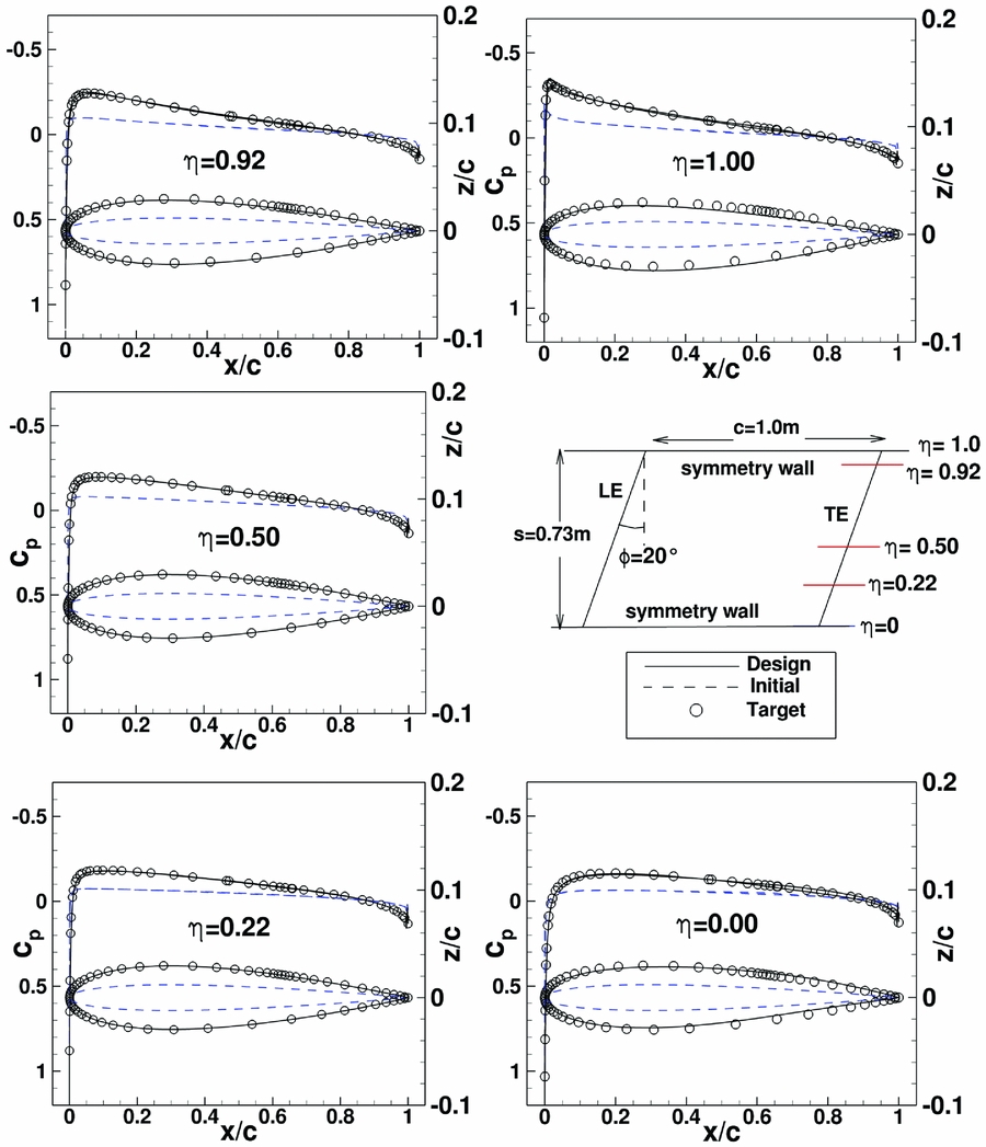
Figure 13. Swept wing redesign case between two symmetry planes with symmetric aerofoils. Initial wing geometry has a symmetrical NACA aerofoil with t/c = 0.024. Target pressure distribution was obtained for wing with NACA0006 aerofoil. Design result for design iteration 8.
Next, a redesign case was studied which involves changes in thickness, camber and twist. In this case both inverse design TSP-equations have to be solved. The previous initial swept wing geometry was used. Free-stream conditions are: M ∞ = 0.18, Rec = 4.19 · 106, α = 0°. The target pressure distribution is obtained using a swept wing with a transonic laminar aerofoil modified for low speed. It is obtained for α = 1°. Since design is performed at α = 0°, in the design the wing surface has to be twisted by one degree. Again, initial and target pressure distribution show a larger variation in spanwise direction near to the symmetry planes. Note also that the differences between initial and target pressure distribution are large. Figure 14 shows the untwisted target wing surface geometry and the wing surface design result. Figure 15 shows pressure distribution results for this redesign case after eight design iterations. A converged design (convergence in both: geometry and pressure distribution) could not be obtained, even with the modified inverse design code. This, despite the use of fine mesh and several design parameter variations. Also the solution method was changed, i.e. solution of modified TSP (equations (10) and (11)) was applied sequentially, by setting alternatively rfa or rfs to zero with the intention to have separate smoothing on the symmetrical and asymmetrical geometry corrections. After eight iterations, the pressure distribution of the designed geometry is very close to the target pressure distribution but close to the walls there are differences between target and designed geometry. For a redesign case, this result is unexpected, since for a unique solution, a good agreement is expected between target and design for both quantities pressure distribution as well as geometry. On the other hand, at wing wall intersections, geometry changes required to obtain a certain geometry distribution are larger than corresponding ones on the wing itself. This is due to the fact that in order to reach the target pressure distribution, the new aerofoil sections close to the wall have to compensate the flow imposed by the wall without altering the wall (except for the intersection). The remaining small differences in the pressure distribution for the rear loading for the complete span (see Fig. 15) are considered uncritical, since usually they disappear with further design iterations. Unfortunately, with further design iterations, the geometry differences at the walls increase, generating regions with larger twist oscillations as shown in Fig. 14. As a consequence, the designed pressure distribution then also deviates from the target pressure distribution. Due to the difficulties for the case with twist changes, for the third redesign case, the previous redesign case was selected but without a twist change between initial and target geometry. It also involves both symmetrical (thickness) and asymmetrical (camber) geometry corrections. Therefore, both modified TSP equations (Equations (10) and (11)) are tested. The initial configuration is the same as in the previous case, but the free-stream conditions for the design are changed to M ∞ = 0.18, Rec = 4.19 · 106, α = 1°. The target pressure distribution is the same as in the previous redesign case. Figure 16 shows results for this redesign case after 15 design iterations. For the design, both the pressure distribution and the wing geometry converge to the target pressure distribution, respectively, target wing geometry.

Figure 14. Swept wing redesign case between two symmetry planes with twist, thickness and camber change. Designed wing surface is given in dark colour shade and target wing geometry (untwisted) in light colour shade.
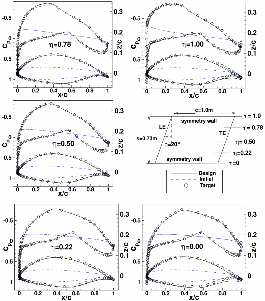
Figure 15. Swept wing between two symmetry planes for a redesign case with twist thickness and camber change. Initial wing geometry has NACA aerofoil with t/c = 0.024. The target pressure distribution was obtained for a wing with a laminar aerofoil for α = 1°. Design results are for design iteration 8. Free-stream condition is M ∞ = 0.18, Rec = 4.19 · 106, α = 0°.

Figure 16. Swept wing between two symmetry planes. Results for a redesign case with thickness and camber changes and without twist change. Initial wing geometry has NACA aerofoil with t/c = 0.024. Target pressure distribution was obtained for wing with a laminar aerofoil for α = 1°. Design results for design iteration 15. Free-stream condition is M ∞ = 0.18, Rec = 4.19 · 106, α = 1°.
A variation of number of considered mirror wings to the left and right of the physical wing was performed. Results show that the influence of mirror wings placed far away from the physical wings is negligible and their consideration does not improve the design convergence. All results presented here were obtained restricting the sum in Equation (19) to only one mirror wing to the left and to the right of the physical wing. The modifications required for the extension of the inverse design code for the two symmetry cases were described in this section and validated with selected redesign cases. An application to a design case is described in Reference HoffroggeRef. 28. Using the modified inverse design code, a constant chord swept wing was designed for a wind tunnel with a spanwise constant (or nearly) constant laminar pressure distribution. The constant pressure corresponds to an infinite swept wing pressure distribution.
7.0 CONCLUSIONS AND OUTLOOK
The DLR 3D inverse design method is an efficient design method based on the numerical solution of the integral inverse small transonic perturbation (TSP) equations. In this work, modifications and extensions have been introduced in the DLR 3D transonic inverse design method. They were described and validated using redesign test cases.
The first modification concerns applications for high transonic Mach numbers close to Mach 1 or transonic flow applications with strong shocks. For cases in which the original inverse design failed to converge to the target pressure distribution, now the modified inverse code provides a converged design. The second modification is the extension of the code to general non-planar wings. Previously the design code was restricted to non-planar wing designs cases with small dihedral or to nacelles (ring wing). A third modification concerns aerofoil/wings designed for wind-tunnel design. For wind-tunnel applications, there are cases where the influence of both lateral wind-tunnel walls (walls in wing spanwise direction) has to be considered in the wing design. For such applications, the solution method of the inverse TSP-equations was extended to two symmetry planes.
Concerning geometry, the used redesigned test cases involved a varying range of complexity, so that both modified inverse TSP equations could be validated separately and together. The most complete changes in geometry between initial and target geometry were for redesign cases in which changes in thickness, camber and angle-of-attack/twist (2D/3D) were required. A converging design was obtained for all redesign test cases, for target pressure as well as for geometry, except for one of the cases considered in the modification taking into account the two symmetry planes. Here the pressure distribution converged initially but not the geometry. This case requires further study
The extensions and modifications introduced have increased robustness and the range of applications of the DLR inverse design method. Here, for the validation of the modifications redesign cases were used, in future real design cases can now be considered.


