2. Equations and boundary conditions

It is known (Faraday Reference Faraday1831) that vibrations of a container filled with a fluid or a system of fluids can lead to parametrically excited waves (Faraday ripple) at a free surface of the fluid or at the fluid interface. Similar phenomena can take place for a drop (bubble) suspended in a medium of differing density when such a system is subjected to vibrations. Since this system possesses eigenfrequencies, at certain ratios between them and the vibration frequency one should expect resonant phenomena. To study the conditions for parametric excitation of the drop oscillations, we consider the following problem.

Let a fluid of density $\rho _{1}$ fill a container, where a drop of different fluid (of density $\rho _{2}$) immiscible with the surrounding medium, is suspended. In the absence of gravity and other external fields, the drop, affected by the surface tension, assumes a spherical shape of radius $R_{0}$. We suppose that the container size and the distance of the drop from its walls by far exceeds the drop size. Let the container undergo translational sinusoidal vibrations with frequency $\omega$ and amplitude $a$. In this case, the inertia forces arise in the reference frame of the container. If the densities of the drop and the surrounding medium are different, these forces are non-uniform, which sets both fluids in motion.

Let the vibration frequency be such that the corresponding sound wavelength is larger than the container size, and the quantity $a\omega$, which determines the order of magnitude of the velocities of the fluids, is small compared with the sound velocity. In this case, the fluids may be considered as incompressible. Additionally, at the first stage of calculations we will neglect the media viscosities, assuming the flow of the fluids to be potential.

In this case, the velocity potentials in both media $\varphi _j$ satisfy the Laplace equations

(2.1)\begin{equation} \varDelta\varphi_j=0, \end{equation}

($j=1,2$; the subscript $1$ refers to the outer fluid, and $2$ to the inner one).

On the rigid walls of the container the impermeability condition is satisfied

(2.2)\begin{equation} \boldsymbol{\nabla}\varphi_1\boldsymbol{\cdot}{\boldsymbol n}=0, \end{equation}

where ${\boldsymbol n}$ is the unit vector normal to the surface.

Since the drop size is assumed to be small as compared with the distance from the container walls, condition (2.2) may be replaced by the condition of vanishing fluid velocity far from the drop

(2.3)\begin{equation} \boldsymbol{\nabla} \varphi_1 \rightarrow 0 \quad \mbox{at}\ r \rightarrow \infty, \end{equation}

where $r$ is the length of the radius vector drawn from the inertial centre of the drop.

The conditions at the drop surface described by equation $G({\boldsymbol r},t)=0$, which has to be determined itself, are the following:

1. (i) The continuity condition for the normal components of fluid velocities

   (2.4)\begin{equation} \left[\boldsymbol{\nabla}\varphi\right]\boldsymbol{\cdot}{\boldsymbol n}=0. \end{equation}

2. (ii) The kinematic condition connecting the displacement of the drop surface with the fluids velocities

   (2.5)\begin{equation} \frac{\partial G}{\partial t}+\boldsymbol{\nabla}\varphi\boldsymbol{\cdot}\boldsymbol{\nabla} G=0. \end{equation}

3. (iii) The condition of the normal stress balance accounting for the inertial forces and surface tension

   (2.6)\begin{equation} \left[\rho\left(\frac{\partial\varphi}{\partial t}+ \frac12\left(\boldsymbol{\nabla}\varphi\right)^2+a\omega^2z\cos\omega t\right)\right] =\alpha\,\textrm{div}\,{\boldsymbol n}+\textrm{const}. \end{equation}

Here, the brackets denote the jump of the value across the interface, $\alpha$ is the surface tension coefficient and the $z$-axis is directed along the vibration axis. Equation (2.6) results from combining Bernoulli's equation with the normal stress balance at the interface. The constant in this equation, generally speaking, can be a function of time, but not coordinates since it results from the integration of the Euler equations describing the flow in the absence of viscosity.

Let us introduce dimensionless variables. We choose the equilibrium radius of a drop as the length scale and the inverse frequency of vibrations $\omega ^{-1}$ and $\omega {R_0}^2$ as the scales for time and the velocity potential, respectively. For the densities of the fluids we take the scale $(\rho _1+\rho _2)$.

Dimensionless equations (2.1) and the boundary conditions (2.3)–(2.5) have the same form as earlier and condition (2.6) takes the form

(2.7)\begin{equation} \left[\tilde\rho\left(\frac{\partial \varphi}{\partial t}+\frac 12 \left(\boldsymbol{\nabla}\varphi\right)^2\right)\right]+ \left[\tilde\rho\right] \tilde a z \cos t=\frac{1}{We}\,\textrm{div}\,{\boldsymbol n} + \textrm{const}. \end{equation}

Here

(2.8a,b)\begin{equation} \tilde\rho_j=\frac{\rho_j}{\rho_1+\rho_2},\quad \tilde a = \frac{a}{R_0} \end{equation}

are the dimensionless densities of two media and the vibration amplitude and

(2.9)\begin{equation} We=\frac{\left(\rho_1+\rho_2\right)\omega^2{R_0}^3}{\alpha} \end{equation}

is the Weber number. Note that, for the scales chosen, the dimensionless densities satisfy the relation

(2.10)\begin{equation} \tilde \rho_1+\tilde\rho_2=1. \end{equation}

Below we omit the tilde for the dimensionless density and vibration amplitude.

Let the amplitude of the imposed vibrations be so small that the inequality

(2.11)\begin{equation} a \ll 1 \end{equation}

holds.

In a real situation in the absence of vibrations the drop oscillations will be damped due to the dissipative effects. Periodic forcing (vibrations, as in our case), in principle, can lead to the resonance excitation of undamped oscillations. Such oscillations can also occur in the case of a small deviation of the vibration frequency from the exact resonance value. In our paper, we consider only small amplitudes of vibrations for which condition (2.11) is satisfied. In this case, the resonance oscillations will take place only at small dissipation of energy. That is why we will restrict ourselves to media with zero or very small viscosities.

Thus, in the problem under consideration arise two different, generally independent, small quantities: the vibration amplitude and the deviation of the frequency from the resonance value. In this situation it is suitable to introduce a formal small dimensionless parameter $\varepsilon$ and to search for the solution of the problem in the form of a power series with respect to this parameter. Let us set

(2.12)\begin{gather} a=\varepsilon a_{1}, \end{gather}

(2.13)\begin{gather}We=We_{0}+\varepsilon We_{1}. \end{gather}

In (2.13) the Weber number, which can be interpreted as the squared vibration frequency, is expanded into a power series with respect to $\varepsilon$ instead of frequency itself. By $We_{0}$ we denote the resonance value of $We$ which is to be determined from the solution of the problem).

Let us consider small deviations of a drop shape from equilibrium

(2.14)\begin{equation} r=1+\varepsilon f(\theta, t). \end{equation}

In (2.14), $r$ and $\theta$ are the spherical coordinates, the polar angle $\theta$ is measured from the vibrations axis. Due to the symmetry of the problem, axisymmetrical flows are considered, and all the variables are assumed to be independent of the azimuthal angle.

As $\varepsilon$ is small (and, consequently, so are the $\varphi _{j}$), the problem may be solved by expanding the variables into power series with respect to $\varepsilon$. Assuming that the $\varphi _{j}$ are of the same order of magnitude as $\varepsilon$, we write down the potential in the form $\varphi _{j}=\varepsilon \tilde {\varphi _{j}}$, where $\tilde {\varphi _{j}}$ is a finite quantity.

The boundary conditions (2.4), (2.5), (2.7) are to be imposed at the drop surface, i.e. at $r=1+\varepsilon f$. Expanding these conditions in Taylor series with respect to the deviation of the drop shape from the spherical one, one obtains the relations to be satisfied at $r=1$. For example, condition (2.4), written in a detailed form, is

(2.15)\begin{equation} r=1+\varepsilon f:\quad \left[{\varepsilon \tilde\varphi _r- \frac{{\varepsilon^2 }}{{r^2 }}f_\vartheta\tilde\varphi_\vartheta}\right]=0, \end{equation}

since for the axisymmetric case and small deviations of the drop shape from the spherical one we have

(2.16a,b)\begin{equation} \boldsymbol{\nabla}\tilde\varphi=\tilde\varphi_{r} \boldsymbol{e}_r+\frac{1}{r}\tilde\varphi_{\vartheta}\boldsymbol{e}_{\vartheta},\quad \boldsymbol{n}=\boldsymbol{e}_{r}-\frac{1}{r} f_\vartheta\boldsymbol{e}_{\vartheta}. \end{equation}

By changing

(2.17)\begin{equation} \left.{\tilde\varphi_r}\right|_{r=1+\varepsilon f}=\left.{\tilde\varphi_r }\right|_{r=1}+ \varepsilon f\left.{\tilde\varphi_{rr}}\right|_{r=1}+O(\varepsilon^2), \end{equation}

we obtain

(2.18)\begin{equation} r = 1:\quad \varepsilon \left[ {\tilde \varphi _r } \right] + \varepsilon ^2 \left[{f\tilde \varphi _{rr} - f_\theta \tilde \varphi _\theta } \right] + O(\varepsilon^3 )=0, \end{equation}

or, dividing by $\varepsilon$, and omitting the tilde for the potential

(2.19)\begin{equation} \varphi_{1r}+\varepsilon (\varphi_{1rr}f-\varphi_{1\theta }f_{\theta})= \varphi_{2r}+\varepsilon (\varphi_{2rr}f-\varphi_{2\theta }f_{\theta}). \end{equation}

Applying the same operations to the boundary conditions (2.5), (2.7) we obtain

(2.20)\begin{align} f_{t}&=\varphi _{2r}+\varepsilon (\varphi _{2rr}f-\varphi _{2\theta}f_{\theta }), \end{align}

(2.21)\begin{align} &\quad -\rho _{2}\left\lbrack \varepsilon \varphi _{2t}+\varepsilon ^{2}\left(\varphi_{2tr}f+ \frac{1}{2}\varphi _{2r}^{2}+\frac{1}{2}\varphi _{2\theta}^{2}\right)\right\rbrack \nonumber\\ &\qquad +\rho _{1}\left\lbrack \varepsilon \varphi _{1t}+\varepsilon^{2} \left(\varphi _{1tr}f+ \frac{1}{2}\varphi _{1r}^{2}+ \frac{1}{2}\varphi_{1\theta }^{2}\right)\right\rbrack \nonumber\\ &\quad =\frac{1}{We}\left[ 2-\varepsilon (2f+\,f_{\theta \theta }+ f_{\theta}\cot \theta )+2\varepsilon ^{2}f(\,f+f_{\theta \theta }+ f_{\theta }\cot\theta )\right] \nonumber\\ &\qquad + (\rho _{2}-\rho _{1})\varepsilon a_{1}\cos \theta\cos t+(\rho _{2}-\rho _{1})\varepsilon ^{2}a_{1}f\cos \theta \cos t+\textrm{const}. \end{align}

Letter subscripts in (2.20)–(2.21) stand for differentiation with respect to the corresponding variables; the curvature of the surface $\textrm {div}\,{{\boldsymbol n}}$ is calculated with an accuracy of up to $\varepsilon ^{2}$.

The summary of the assumptions used in our theory in the inviscid case is the following:

(2.22a–c)\begin{equation} \omega \ll 2 {\rm \pi}c/R_0,\quad a \ll R_0,\quad We-We_0 \ll 1 . \end{equation}

3. Forced oscillations of the drop

At zeroth order, the constant in (2.21) is evaluated, and to the next order we obtain the following problem for the determination of the fluid velocities and the drop shape (the corresponding variables of the linear problem are capitalized):

(3.1)\begin{equation} \varDelta \varPhi _{j}=0, \end{equation}

at $r\rightarrow \infty$

(3.2)\begin{equation} \boldsymbol{\nabla}\varPhi_{1}=0, \end{equation}

and at $r=1$

(3.3)\begin{gather} F_{t}=\varPhi_{2r}, \end{gather}

(3.4)\begin{gather}\varPhi_{1r}=\varPhi _{2r}, \end{gather}

(3.5)\begin{gather}-\rho _{2}\varPhi _{2t}+\rho _{1}\varPhi _{1t}-(\rho _{2}-\rho _{1})a_{1}\cos \theta \cos t=-\frac{1}{We}\left( 2F+F_{\theta \theta }+F_{\theta }\cot \theta \right). \end{gather}

Here, now $\varPhi$ is the leading part of the velocity potential.

The solution of the linear problem (3.1)–(3.5) is

(3.6)\begin{gather} F=\tfrac{2}{3}\mu \cos \theta \cos t, \end{gather}

(3.7)\begin{gather}\varPhi _{1}=\tfrac{1}{3r^{2}}\mu \cos \theta \sin t, \end{gather}

(3.8)\begin{gather}\varPhi _{2}=-\tfrac{2}{3}\mu r\cos \theta \sin t, \end{gather}

where the following notation is introduced

(3.9)\begin{equation} \mu =\frac{3(\rho _{1}-\rho _{2})}{2\rho _{2}+\rho _{1}}a_{1}. \end{equation}

Thus, to the first order with respect to $\varepsilon$ we obtain the solution which corresponds to the translational oscillation of the drop with the amplitude $2\mu \varepsilon /3$ and the frequency equal to that of the container oscillations. Moreover, the shape of the drop does not change. The amplitude of these oscillations becomes zero at $\rho _{1}=\rho _{2}$, since in this case the inertial forces are uniform. The phase of oscillations of the drop is determined by the density difference: the oscillations of a denser drop occur in the counterphase relative to the container oscillations, the phase of oscillations of a lighter drop is the same as that of the container.

4. Stability analysis

To analyse the stability of the obtained solution, it is convenient to transit to the reference framework moving with the drop. In this framework, the basic solution (3.6)–(3.8) has the form

(4.1)\begin{gather} F=0, \end{gather}

(4.2)\begin{gather}\varPhi _2=0, \end{gather}

(4.3)\begin{gather}\varPhi_1=\tfrac{2}{3} \mu\left(r+\tfrac 1{2r^2}\right)\cos\theta\sin t. \end{gather}

The problem for the perturbations of the basic solution (4.1)–(4.3) is obtained from (2.1)–(2.3) and (2.20)–(2.21) in the linear approximation, taking into account the modification of the inertial forces with the transition to the new reference frame. The perturbations of the velocity potentials satisfy the Laplace equations, they vanish far from the drop (for the outer medium) and satisfy the following conditions at the drop surface, $r=1$:

(4.4)\begin{gather} f_t=\varphi_{2r}, \end{gather}

(4.5)\begin{gather}\varphi_{2r}-\varphi_{1r}=2\mu\sin t\left(\,f\cos\theta+ \tfrac 12 f_\theta\sin\theta \right), \end{gather}

(4.6)\begin{gather}\rho_1\varphi_{1t}-\rho_2\varphi_{2t}+\frac{1}{We}\left(2f +f_{\theta\theta}+f_\theta\cot\theta\right)=\mu\rho_1(\varphi_{1\theta} \sin\theta\sin t+f\cos\theta\cos t). \end{gather}

For the perturbations we use the same notations as for the functions themselves.

The solution to the Laplace equation that vanishes at infinity and does not have any singularities at the drop centre, has the form

(4.7)\begin{gather} \varphi_1=\sum\frac{A_k(t)}{r^{k+1}}P_k(\cos\theta), \end{gather}

(4.8)\begin{gather}\varphi_2=\sum B_k(t)r^k P_k(\cos\theta). \end{gather}

At the same time, the following equality holds

(4.9)\begin{equation} f=\sum f_k P_k(\cos\theta), \end{equation}

where $P_k$ are Legendre polynomials of $k$th order.

Substituting (4.7)–(4.9) into (4.4)–(4.6), at the zeroth order with respect to $\mu$ we arrive at the known problem (Landau & Lifshitz Reference Landau and Lifshitz1987) of the eigen-oscillations of the drop. In this case, the spectrum of eigenfrequencies is

(4.10)\begin{equation} \varOmega_k^2=\frac{1}{We}\frac{k(k^2-1)(k+2)}{\rho_1k+\rho_2(k+1)}, \end{equation}

where $k\geq 2$ since the case $k=0$ is impossible because of incompressibility of the fluids, and $k=1$ corresponds to a uniform displacement of the drop, and not to oscillations.

Analysis of (4.4)–(4.6) at the next order shows that, in principle, the resonant excitation of harmonics is possible under the following synchronism condition:

(4.11)\begin{equation} \varOmega_{k+1}+\varOmega_{k}=1. \end{equation}

Let the value of the Weber number be in such a range that the synchronism condition (4.11) is satisfied for some pair of modes. Then, all the harmonics of the solution (4.7)–(4.9), except for the $k$th and $(k+1)$th, are non-resonant and, consequently, to find the resonance conditions it is sufficient to restrict ourselves to just this pair of the harmonics of (4.7)–(4.9), assuming that

(4.12)\begin{gather} f=f_kP_k+f_{k+1}P_{k+1}, \end{gather}

(4.13)\begin{gather}\varphi_1=\frac{A_k}{r_{}^{k+1}}P_k+\frac{A_{k+1}}{r^{k+2}}P_{k+1}, \end{gather}

(4.14)\begin{gather}\varphi_2=B_kr^kP_k+B_{k+1}r^{k+1}P_{k+1}. \end{gather}

Here, the argument in Legendre polynomials is $\cos \theta$; $f_k$, $A_k$ and $B_k$ are the functions of time.

Substitution of (4.12)–(4.14) into (4.4)–(4.6) after omitting non-resonant harmonics yields the set of ordinary differential equations

(4.15)\begin{gather} \stackrel{.}{f}_k=kB_k, \end{gather}

(4.16)\begin{gather}\stackrel{.}{f}_{k+1}=(k+1)B_{k+1}, \end{gather}

(4.17)\begin{gather}kB_k+(k+1)A_k=-\mu \frac{k(k+1)}{2k+3}f_{k+1}\sin t, \end{gather}

(4.18)\begin{gather}(k+1)B_{k+1}+(k+2)A_{k+1}=\mu\frac{(k+1)(k+2)}{2k+1}f_k\sin t, \end{gather}

(4.19)\begin{gather}\rho_1\stackrel{.}{A}_k-\rho_2\dot B_k-\frac{\beta_k}{We}f_k=\rho_1 \mu \frac{k+1}{2k+3}\left[-(k+2)A_{k+1}\sin t+f_{k+1}\cos t\right], \end{gather}

(4.20)\begin{gather}\rho_1\stackrel{.}{A}_{k+1}-\rho _2\dot B_{k+1}-\frac{\beta_{k+1}}{We} f_{k+1}=\rho_1\mu\frac{k+1}{2k+1}\left[kA_k\sin t+f_k\cos t\right]. \end{gather}

Here, overdots stand for differentiation of functions with respect to time and we denote

(4.21)\begin{equation} \beta_k=(k-1)(k+2). \end{equation}

The set (4.15)–(4.20) can be reduced to two equations for $f_k$ and $f_{k+1}$

(4.22)\begin{gather} -\alpha_k\stackrel{..}{f}_k-\frac{\beta_k}{We}f_k=\rho_1\mu \frac{2k+1}{2k+3} \left(\stackrel{.}{f}_{k+1}\sin t+f_{k+1}\cos t\right), \end{gather}

(4.23)\begin{gather}-\alpha_{k+1}\stackrel{..}{f}_{k+1}-\frac{\beta_{k+1}}{We}f_{k+1}= -\rho_1\mu \stackrel{.}{f}_k\sin t, \end{gather}

where

(4.24)\begin{equation} \alpha_k=\frac{\rho_2}k+\frac{\rho_1}{k+1}. \end{equation}

To study (4.22)–(4.23), it is convenient to use the multiple scale method (Nayfeh Reference Nayfeh1981). In accordance with it, we introduce a hierarchy of time scales, so that the time derivative is represented as the series

(4.25)\begin{equation} \frac\partial{\partial t}=\frac{\partial}{\partial t_0}+ \varepsilon \frac{\partial}{\partial t_1}+\cdots. \end{equation}

The functions $f_k$ and $f_{k+1}$ are also presented in series form

(4.26)\begin{gather} f_k={f_k}^{(0)}+\varepsilon {f_k}^{(1)}+\cdots, \end{gather}

(4.27)\begin{gather}f_{k+1}={f_{k+1}}^{(0)}+\varepsilon {f_{k+1}}^{(1)}+\cdots. \end{gather}

Substitution of series (4.25)–(4.27) into the set of equations (4.22)–(4.23) yields, to the leading order,

(4.28)\begin{gather} \stackrel{..}{{f}_k}^{(0)}+\,{\varOmega_k}^2 {f_k}^{(0)}=0, \end{gather}

(4.29)\begin{gather}\stackrel{..}{f}_{k+1}^{(0)}+\,\varOmega_{k+1}^2\, f_{k+1}^{(0)}=0, \end{gather}

i.e. the solutions are independent oscillations with the frequencies $\varOmega _k$ and $\varOmega _{k+1}$, defined by (4.10). Thus,

(4.30)\begin{gather} {f_k}^{(0)}=C\exp(\textrm{i}\varOmega_kt_0)+C^*\exp(-\textrm{i}\varOmega_kt_0), \end{gather}

(4.31)\begin{gather}f_{k+1}^{(0)}=D\exp(\textrm{i}\varOmega_{k+1}t_0)+D^*\exp(-\textrm{i}\varOmega_{k+1}t_0), \end{gather}

where ‘$*$’ stands for complex conjugation, the amplitudes $C$ and $D$ do not depend on the ‘fast’ time $t_0$, but, generally speaking, are functions of ‘slow’ time $t_1$.

To the next order, (4.22)–(4.23) with allowance for (4.25)–(4.27) yield

(4.32)\begin{gather} -\alpha _{k}\frac{\partial ^{2}f_{k}^{(1)}}{\partial t_{0}^{2}}-2\alpha _{k} \frac{\partial ^{2}f_{k}^{(0)}}{\partial t_{0}\partial t_{1}}- \frac{\beta _{k}}{We_{0}}f_{k}^{(1)}+\frac{\beta _{k}}{We_{0}^{2}}We_{1}f_{k}^{(0)} \nonumber\\ \quad = \rho_{1}\mu\frac{2k+1}{2k+3}\left(\frac{\partial f_{k+1}^{(0)}}{\partial t_{0}} \sin t_{0}+f_{k+1}^{(0)}\cos t_{0}\right), \end{gather}

(4.33)\begin{gather} -\alpha _{k+1}\frac{\partial ^{2}f_{k+1}^{(1)}}{\partial t_{0}^{2}}-2\alpha_{k+1} \frac{\partial ^{2}f_{k+1}^{(0)}}{\partial t_{0}\partial t_{1}}- \frac{\beta _{k+1}}{We_{0}}f_{k+1}^{(1)}+\frac{\beta _{k+1}}{We_{0}^{2}}We_{1}f_{k+1}^{(0)}= -\rho_{1}\mu \frac{\partial f_{k}^{(0)}}{\partial t_{0}} \sin t_{0}. \end{gather}

Here, ${We}_{0}$ is the value of the Weber number at which the synchronism condition (4.11) is satisfied and $\varepsilon {We}_{1}$ is a small deviation from this value.

If condition (4.11) is satisfied, the non-uniformities of equations (4.32)–(4.33), which determine $f_k$ and $f_{k+1}$, contain the resonance terms. The requirement of the absence of secular solutions to this set determines the evolution of $C$ and $D$ as

(4.34)\begin{gather} -2\textrm{i}\alpha_k\varOmega_k\frac{\partial C}{\partial t_1}+ \frac{\beta_k}{{{We}_0}^2} {We}_1C=\frac 12 \rho_1 \mu\frac{2k+1}{2k+3}(1-\varOmega_{k+1})D^*, \end{gather}

(4.35)\begin{gather}2\textrm{i}\alpha_{k+1}\varOmega_{k+1}\frac{\partial D^*}{\partial t_1} +\frac{ \beta_{k+1}}{{{We}_0}^2}{We}_1D^*=\frac 12 \rho_1\mu\varOmega_k C. \end{gather}

Since the set (4.34)–(4.35) is linear, it admits a solution proportional to $\exp (\kappa t_1)$. Substituting this solution into (4.34)–(4.35), one gets the set of linear algebraic equations for the corresponding amplitudes. These solutions are non-zero if the determinant equals zero. This condition yields the equation for the increment $\kappa$

(4.36)\begin{align} & 4\alpha_k\alpha_{k+1}\varOmega_k\varOmega_{k+1}\kappa^2+2\textrm{i}\frac{{We}_1} {{We}_0^2} \kappa\left(\alpha_{k+1}\varOmega_{k+1}\beta_k-\alpha_k\varOmega_k \beta_{k+1}\right) \nonumber\\ &\quad +\beta_k\beta_{k+1}\frac{{We}_1^2}{{We}_0^4}-\frac{\mu^2}{4} \frac{2k+1}{2k+3}\varOmega_k^{2} {\rho_1}^2=0. \end{align}

In the parameter range where the increment $\kappa$ is positive (instability area) the solutions of (4.34)–(4.35) are exponentially growing and expansions (4.26), (4.27) become invalid at large time. From algebraic equation (4.36) it follows that the solutions of equations (4.34)–(4.35) are growing if the discriminant of (4.36) is positive, i.e. if

(4.37)\begin{equation} {\rho_1}^2 \mu^2\frac{2k+1}{2k+3}\varOmega_k^2\alpha_k\alpha_{k+1} \varOmega_k \varOmega_{k+1}>\frac{{We}_1^2}{{We}_0^4}\left(\alpha_k \varOmega_k\beta_{k+1} +\alpha_{k+1}\varOmega_{k+1}\beta_k\right)^2. \end{equation}

6. Accounting for small viscosity

The threshold of excitation of parametric oscillations in figure 1 equals zero at ${We}_1=0$, i.e. when the resonance condition (4.11) is satisfied identically. The absence of a finite threshold for parametric excitation is due to the inviscid media model.

For fluids of low viscosity $\nu _j$, when the condition

(6.1)\begin{equation} \frac{\nu_j}{\omega {R_0}^2}\ll1 \end{equation}

holds, one can account for the viscous dissipation with the aid of the following scheme. Since we assume that inequality (6.1) is satisfied, then the viscous corrections to the eigenfrequency for the spherical $k$th mode (for comparable densities of media) to the leading order have the form (Chandrasekhar Reference Chandrasekhar1959)

(6.2)\begin{equation} \omega_{1k}=\varepsilon (\textrm{i}-1)\gamma_k, \end{equation}

where

(6.3)\begin{equation} \gamma_k=\frac 12\sqrt{\frac{\varOmega_k}2}(2k+1)^2 \frac{W\,\textrm{e}^{-(1/4)}} {\alpha_k} \frac{\rho_1\rho_2\sqrt{\nu_1\nu_2}}{\rho_1\sqrt{\nu_1}+ \rho_2 \sqrt{\nu _2}}. \end{equation}

Here, $\nu _j$ denote dimensionless analogues of the viscosity coefficients scaled with $\sqrt {\alpha {R_0}/(\rho _1+\rho _2)}$.

We remark that the order of magnitude for the viscosity coefficients is explicitly predetermined. It follows from (6.2) that, in the approximation applied, one should take the viscosity as the small quantity of the second order.

As seen from (6.3), the correction depends on the mode number, and its presence, since $\omega _{1k}$ is complex, leads not only to the damping of eigen-oscillations but also to the viscous shift of their frequencies.

Since we consider low viscosity fluids, then $\gamma _{k}$ is a small quantity and to account for the viscous dissipation it suffices to introduce this quantity in (4.34)–(4.35) just replacing

(6.4)\begin{equation} \frac{\partial }{\partial t_{1}}\rightarrow \frac{\partial } {\partial t_{1}}-\textrm{i}(\textrm{i}-1)\gamma _{k}. \end{equation}

Such a way of accounting for the weak dissipation is certainly approximate and has to be looked at as a phenomenological one. It does not allow for nonlinear dissipative effects and requires an additional assumption regarding the order of the damping coefficient smallness. However, a quite similar approach is traditionally used in the studies of waves at the free surface or interface, particularly, including studies of parametrically excited oscillations (see, for example, Miles & Henderson Reference Miles and Henderson1990; Edwards & Fauve Reference Edwards and Fauve1994; Kumar & Tuckerman Reference Kumar and Tuckerman1994; Christiansen, Alstrom & Levinsen Reference Christiansen, Alstrom and Levinsen1995; Lyubimova et al. Reference Lyubimova, Ivantsov, Garrabos, Lecoutre and Beysens2019) and often allows one to obtain qualitatively good results. In Kumar & Tuckerman (Reference Kumar and Tuckerman1994) the instability threshold and critical wavelength obtained using a phenomenological approach and by numerical simulation based on the full Navier–Stokes equations (FHS) are compared. It is found that the wavelengths predicted by the two approaches do not differ significantly for low viscosity. The authors also compare the results of the phenomenological and FHS approaches with the experimental results obtained for a viscous glycerine–water mixture in contact with air in Edwards & Fauve (Reference Edwards and Fauve1993). It is found that both the phenomenological and FHS approaches agree reasonably well with the experimentally measured wavelengths. In Lyubimova et al. (Reference Lyubimova, Ivantsov, Garrabos, Lecoutre and Beysens2019), the Faraday waves on a band pattern formed in two-phase systems near the critical point under zero gravity conditions were studied. Comparison of the instability threshold values obtained analytically using a phenomenological approach, numerically by direct numerical simulation based on the Navier–Stokes equations and experimentally has shown good agreement.

Further calculations for the region of parametric resonance are carried out according to the above-described scheme. The neutral curve obtained in this way has the following form in the coordinates $a_{1},{We}_{1}$:

(6.5)\begin{align} & \gamma _{k}\gamma _{k+1}\left[ \frac{(\alpha _{k}\varOmega _{k}\beta _{k+1}+\alpha _{k+1} \varOmega _{k+1}\beta _{k})^{2}}{\alpha _{k}\alpha _{k+1}\varOmega _{k}\varOmega _{k+1} (\gamma _{k}+\gamma _{k+1})^{2}} \frac{{We}_{1}^{2}}{{We}_{0}^{4}}+ \frac{4(\alpha _{k} \varOmega _{k}\beta _{k+1}+\alpha _{k+1}\varOmega _{k+1} \beta _{k})}{\gamma _{k}+\gamma _{k+1}}\frac{{We}_{1}}{{We}_{0}^{2}} \right] \nonumber\\ &\quad +8\gamma _{k}\gamma _{k+1}\alpha _{k}\alpha _{k+1}\varOmega _{k}\varOmega _{k+1}- \frac{9\rho _{1}^{2}(\rho _{2}-\rho _{1})^{2}} {4(2\rho _{2}+\rho _{1})^{2}} a_{1}^{2} \frac{2k+1}{2k+3} {\varOmega _{k}}^{2}=0. \end{align}

Viscous dissipation, if taken into account, leads to two different effects. First, the parametric excitation for the resonance becomes that of a finite amplitude type so that the oscillations arise (in the minimum of the neutral curve) when $a_{1}$ exceeds some critical value

(6.6)\begin{equation} a^{\ast }=\frac{4(2\rho _{2}+\rho _{1})}{3\rho _{1}\varOmega _{k}|\rho _{2}-\rho _{1}|} \sqrt{\frac{2k+3}{2k+1}\gamma _{k}\gamma _{k+1}\alpha _{k}\alpha _{k+1}\varOmega _{k}\varOmega _{k+1}}. \end{equation}

Second, a viscous shift of the frequency from the value determined by (4.11) takes place. The minimum of the neutral curve occurs not at ${We}_{1}=0$ but when it assumes the value

(6.7)\begin{equation} {We}_{1\ast }=-\frac{2{We}_{0}^{2}(\gamma _{k}+\gamma _{k+1})\alpha _{k}\alpha _{k+1} \varOmega _{k}\varOmega _{k+1}}{\alpha _{k}\varOmega _{k} \beta _{k+1}+\alpha _{k+1} \varOmega _{k+1}\beta _{k}}. \end{equation}

The threshold value of the vibration amplitude (6.6) decreases as the number $k$ grows. However, the threshold value of the amplitude of the vibration velocity, which is equal the product $a\omega$ and experimentally characterizes the power loss at the vibrating plate, increases with $k$. This means that the most easily excited resonance is the one where the second and third modes of eigen-oscillations interact.

Formula (6.5) has one important feature. When the viscosity tends to zero, it does not turn into (5.1), yielding instead

(6.8)\begin{equation} a_{1}=\pm \varGamma _{k}q_{k}{We}_{1}, \end{equation}

where

(6.9)\begin{equation} {\varGamma _{k}}^{2}=\frac{4\alpha _{k}\alpha _{k+1}\sqrt{\varOmega _{k} \varOmega _{k+1}} (2k+1)^{2}(2k+3)^{2}}{\left[ \alpha _{k+1} \sqrt{\varOmega _{k}}(2k+1)^{2}+\alpha _{k}\sqrt{\varOmega _{k+1}} (2k+3)^{2}\right] ^{2}}. \end{equation}

The value $\varGamma _k$ is always less than unity, therefore the straight lines (6.8) are inclined to the ${We}_1$-axis more than those given by (5.1). Thus, the presence of an infinitesimal dissipation considerably changes the resonance properties as compared with the case $\nu _1=\nu _2=0$. Cases of such paradoxical behaviour are known in the mechanics of elastic discrete systems (Schmidt Reference Schmidt1975). However, the situation is different in the case of Faraday ripple at a flat interface and for the Mathieu equation, which makes this result paradoxical. In the next subsection we show that, in reality, the increase of the width of the instability zone including a small viscosity is a general situation whereas Faraday ripple is a particular case where the destabilizing effect is reduced due to the symmetry properties of the system.

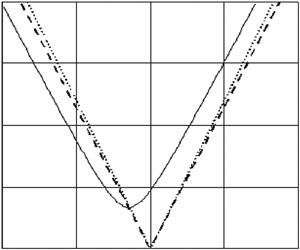
In figure 3 the stability map is presented for the second and third resonant modes for the dimensionless densities $\rho _1=0.555$, $\rho _2=0.445$. Dotted lines correspond to $\nu _1=\nu _2=0$ (that is the same resonance as in figure 1), dashed lines correspond to $\nu _1,\nu _2\rightarrow 0$. Solid line is plotted for a kerosene drop of the radius $1\ \textrm {cm}$ in water. As one can see, at small deviations of ${We}$ from the resonance value (that is, at small $\varepsilon {We}_1$), viscosity stabilizes the equilibrium by increasing the excitation threshold as compared with the case of inviscid media. However, at further deviation of ${We}$ from the resonance value, the solid line crosses the dashed and dotted lines. This means that, in these regions, the viscosity plays a destabilizing role.

Figure 3. First resonance zone ($k=2$) for different dimensionless viscosities: dotted lines - $\nu _1=0$, $\nu _2=0$; dashed lines - $\nu _1 =10^{-6}$, $\nu _2 =10^{-6}$; solid lines - $\nu _1=0.00190$, $\nu _2=0.00133$.

If the density of the drop is very small as compared with the density of the surrounding medium (a gaseous bubble in a liquid matrix), one should take a different value for the damping coefficient. In this case, instead of (6.2)–(6.3) we take

(6.10)\begin{equation} \omega_{1k}=\textrm{i}\gamma_k, \quad \gamma_k=\nu_1(2k+1)(k+2). \end{equation}

Then we obtain

(6.11)\begin{equation} a^{\ast 2}=\frac{16\varOmega _{k+1}{\nu_{1}}^{2}(k+3)(2k+1)(2k+3)(3k+5)} {9\varOmega _{k}(k+1)(3k+2)}. \end{equation}

As one can see, unlike the case of fluids with comparable densities, the resonance excitation threshold is now proportional to the viscosity and not to its square root as in (6.6). That is, in the low viscosity approximation, oscillations of a gas bubble are induced by the container oscillations with smaller amplitude than the oscillations of a heavy drop. There is no viscous shift of frequency in this case.

Thus, the vibrations of a container lead to excitation of a specific parametric resonance owing to the coupling of the neighbouring modes of the eigen-oscillations of the drop suspended in a fluid of different density. The threshold value of the vibration velocity amplitude for this resonance is determined by the viscous dissipation and grows with the increase of the number of resonating modes and, consequently, with the increase of the frequency of the container oscillations.

7. On the paradoxical influence of the viscosity on parametric instability

Unlike a usual resonance of forced oscillations, for the parametric resonance the transfer of energy from an external source does not occur directly but is due to the control of the interaction of different modes of eigen-oscillations. In this case, for weak interaction, the synchronism conditions should be satisfied. If there are two modes of eigen-oscillation with frequencies $\omega _1$ and $\omega _2$ interacting with the external source with frequency $\varOmega$, then

(7.1)\begin{equation} \varOmega = \omega_1 + \omega_2. \end{equation}

A deviation from exact synchronism does not prevent the resonance, but requires a finite amplitude of forcing, which could provide synchronization of oscillations. For two modes with frequencies only slightly different from those satisfying condition (7.1), in the absence of forcing and dissipation, we can derive equations for a slow evolution of amplitudes

(7.2)\begin{gather} \stackrel{.}{X} + \textrm{i} \delta_1 X =0, \end{gather}

(7.3)\begin{gather}\stackrel{.}{Y} + \textrm{i} \delta_2 Y =0, \end{gather}

where $\delta _1$ and $\delta _2$ are frequency mismatch parameters. In the case of interaction with an external energy source, the equations are modified

(7.4)\begin{gather} \stackrel{.}{X} + \textrm{i} \delta_1 X +\eta_1 Y = 0, \end{gather}

(7.5)\begin{gather}\stackrel{.}{Y} + \textrm{i} \delta_2 Y +\eta_2 X = 0. \end{gather}

Here, $\eta _1$ and $\eta _2$ are parameters proportional to the amplitude of forcing. Solutions to equation (7.4) are proportional to $\exp (\lambda t)$ where the growth rate $\lambda$ is determined by the characteristic equation

(7.6)\begin{equation} \lambda^2 +\textrm{i}(\delta_1+\delta_2)\lambda - \delta_1 \delta_2 - \eta_1 \eta_2= 0. \end{equation}

Dependence of the real part of growth rate on the parameter of forcing $\eta =\eta _1\eta _2$ is plotted in figure 4.

Figure 4. Dependence of the real part of growth rate on the parameter of forcing $\eta =\eta _1\eta _2$.

Critical (threshold) amplitude for excitation $\eta _*$ differs from zero for different mismatches of two interacting modes

(7.7)\begin{equation} \eta_*= \tfrac{1}{4}(\delta_1-\delta_2)^2. \end{equation}

If $\eta <\eta _*$, the growth rate is purely imaginary, which corresponds to the absence of synchronization.

To account for dissipation, one needs to add dissipative terms into (7.4)

(7.8)\begin{gather} \stackrel{.}{X} + \textrm{i} \delta_1 X +\sigma_1 X + \eta_1 Y = 0, \end{gather}

(7.9)\begin{gather}\stackrel{.}{Y} + \textrm{i} \delta_2 Y +\sigma_2 Y + \eta_2 X = 0. \end{gather}

Growing solutions of (7.8)–(7.9) appear when the parameter $\eta$ reaches the threshold value $\eta _d$

(7.10)\begin{equation} \eta_d=\sigma_1 \sigma_2 \left[ 1+ \left( \frac{\delta_1-\delta_2}{ \sigma_1+\sigma_2} \right) ^2 \right]. \end{equation}

For $\sigma _1 =\sigma _2 =\sigma$ we obtain from (7.10) $\eta = \eta _e$, where

(7.11)\begin{equation} \eta_e =\tfrac{1}{4} \left( \delta_1 - \delta_2 \right)^2 + \sigma^2 = \eta_* + \sigma^2, \end{equation}

i.e. $\eta _e > \eta _*$; at equal damping coefficients the dissipation increases the instability threshold. However, at $\sigma _1\ne \sigma _2$, as one can see from (7.10), $\eta _d$ can assume any small values. Moreover, for small enough but different damping coefficients, $\eta _d$ is necessarily less than $\eta _*$. Indeed, by introducing the notation $\sigma _2/\sigma _1=q$ we can rewrite (7.10) in the form

(7.12)\begin{equation} \eta_d=\frac{4q}{(1+q)^2} \eta_* + q {\sigma_1}^2, \end{equation}

from which we have

(7.13)\begin{equation} \eta_d-\eta_*=-\left(\frac{1-q}{1+q}\right)^2 \eta_* + \sigma_1 \sigma_2. \end{equation}

The right-hand side of (7.13) is negative at any $k \ne 1$ and with small enough product $\sigma _1\sigma _2$. Typical dependence of the real part of growth rate on $\eta$ is presented in figure 5.

Figure 5. Typical dependence of the real part of the growth rate on $\eta$.

Thus, the extension of the parameter range for excitation of parametric resonance when weak dissipation is accounted for is a general result. The situation is different only in some particular cases when $\sigma _1 = \sigma _2$. One of these particular cases is the excitation of Faraday ripple at a flat surface of a fluid. In that case, two interacting modes are two waves propagating in opposite directions. Due to the symmetry of the problem, for these waves $\delta _2 = -\delta _1$ and $\sigma _2 = \sigma _1$ and accounting for the dissipation results in a decrease of the instability range. In the situation under consideration, two interacting modes are different modes of eigen-oscillations of a drop with different spatial structures and consequently different damping coefficients.

The paradoxical extension of the instability domain in the parameter space under the influence of infinitesimal dissipative forces is also known for linear, autonomous, non-conservative mechanical systems (see, for example, Kirillov Reference Kirillov2007).

Declaration of interests

The authors report no conflict of interest.