


1. Introduction
Research on thermoacoustic instabilities has led to significant advances in the understanding of the driving and coupling processes at stake. This effort, motivated by practical issues, has been aimed in particular at developing reduced-order models and tools that allow the prediction of these undesired phenomena, enable the design of systems free of instabilities or help reduce the amplitude of oscillations if they occur. In recent years, research has been specifically directed at instabilities coupled by azimuthal modes in annular combustors, a geometry that is found in many aeroengines and gas turbines (O’Connor, Acharya & Lieuwen Reference O.’Connor, Acharya and Lieuwen2015; Poinsot Reference Poinsot2017; Schuller, Poinsot & Candel Reference Schuller, Poinsot and Candel2020). To describe combustion systems’ dynamics, one needs to characterize the flame response to acoustic disturbances. This response is usually represented by a flame transfer or describing function (FTF and FDF, respectively), which links, through a gain and a phase, the relative heat release rate (HRR) fluctuations to an input, that may be relative volume flow rate disturbances, relative equivalence ratio fluctuations or pressure fluctuations (Dowling Reference Dowling1997; Noiray et al. Reference Noiray, Durox, Schuller and Candel2008; Schuller et al. Reference Schuller, Poinsot and Candel2020). The describing function concept is the nonlinear extension of the FTF and is used to capture the effects of the oscillation amplitude on the flame response. It can suitably describe the saturation process of the HRR fluctuations which takes place at high modulation amplitudes, reducing the flames’ response and explaining why oscillations reach a limit cycle after a phase of growth (Dowling Reference Dowling1997; Lieuwen Reference Lieuwen2003; Balachandran et al. Reference Balachandran, Ayoola, Kaminski, Dowling and Mastorakos2005; Noiray et al. Reference Noiray, Durox, Schuller and Candel2008). Flame describing function measurements are available in the literature, but they are often limited to weakly nonlinear cases. Experiments and numerical simulations documenting the nonlinear flame response at high modulation amplitudes, close to those observed during limit-cycle oscillations (Wolf et al. Reference Wolf, Staffelbach, Gicquel, Müller and Poinsot2012; Prieur et al. Reference Prieur, Durox, Schuller and Candel2018), are less common, and this lack of knowledge has been replaced by a modelling of the nonlinear behaviour of the HRR fluctuations at high modulation amplitudes to allow an examination of the evolution to limit cycles.
In the present article, we use recent experiments (Alhaffar et al. Reference Alhaffar, Latour, Patat, Durox, Renaud, Blaisot, Candel and Baillot2024) in the annular combustor MICCA-Spray, which will be designated from here on as MICCA, to propose an alternative representation of the HRR fluctuations in terms of the pressure oscillation amplitude. This new formulation is employed in a generic problem to analyse the evolution to limit cycle using slow-flow variable equations. This study then builds upon the modelling framework proposed by Ghirardo, Juniper & Moeck (Reference Ghirardo, Juniper and Moeck2016), which, in combination with the recent flame response measurements obtained in MICCA, is applied to predict the limit-cycle oscillation amplitudes for a set of staging configurations investigated in Latour et al. (Reference Latour, Durox, Renaud and Candel2024a ). Exploiting the large experimental dataset collected in MICCA together with dynamical equations, this work aims to address the following issues:
-
(i) Can one define an alternative representation of the HRR nonlinearity as a function of the level of oscillation that is more flexible and more easily adaptable to experimental flame dynamics data than current models?
-
(ii) Using the slow variable equations in combination with the new representation of the flame response, is it possible to predict the various limit-cycle amplitudes for the different staging configurations and retrieve the experimental trends and data?
-
(iii) Finally, can one derive an expression for the growth rate from the slow-flow variables’ dynamical equations and does this expression match with another previously obtained from acoustic energy balance principles (Latour et al. Reference Latour, Durox, Renaud and Candel2024a )?
At this point, it is natural to review the literature, but for brevity, we only consider investigations dealing with the modelling of HRR fluctuations in terms of pressure fluctuations and that are specifically aimed at analysing the behaviour of annular combustors. In a seminal investigation, Noiray, Bothien & Schuermans (Reference Noiray, Bothien and Schuermans2011) propose an expression for the HRR fluctuations,
 ${\dot Q}^{\prime}$
, in the form of a third-order polynomial of the pressure disturbances
${\dot Q}^{\prime}$
, in the form of a third-order polynomial of the pressure disturbances
 $p$
:
$p$
:
 ${\dot Q}^{\prime}(p)=\beta p- \kappa p^3$
, with
${\dot Q}^{\prime}(p)=\beta p- \kappa p^3$
, with
 $\beta$
and
$\beta$
and
 $\kappa$
, the linear and saturation coefficients, respectively. When this expression is injected in the wave equation representing the system dynamics and the pressure field is projected on the normal modes, it is found that the modal amplitudes satisfy second-order differential equations that behave like coupled Van der Pol oscillators and feature a finite amplitude limit cycle. This is then used to analyse various issues, like the nature of the coupling mode and symmetry breaking. One difficulty with this kind of modelling is that the polynomial expression matches experimental data when the amplitudes of oscillation are small, but diverges from the measurements when the amplitude takes large values, as indicated in the same article, by making use of data from Balachandran et al. (Reference Balachandran, Ayoola, Kaminski, Dowling and Mastorakos2005). This difficulty was also pointed out by Prieur et al. (Reference Prieur, Durox, Schuller and Candel2018), using signals from strong instability bursts in an annular combustor, where the relation between the relative HRR and the pressure amplitude was found to be quasi-linear. Using the same flame response model but introducing a stochastic forcing term, Noiray & Schuermans (Reference Noiray and Schuermans2013) were then able to account for turbulence effects, inherent to high-power combustors, and in particular for the switching between spinning and standing modes observed in experiments and numerical simulations, which could not be retrieved with a purely deterministic approach. Another extension of this model by Ghirardo & Juniper (2013) was meant to account for the HRR dependence on the azimuthal velocity,
$\kappa$
, the linear and saturation coefficients, respectively. When this expression is injected in the wave equation representing the system dynamics and the pressure field is projected on the normal modes, it is found that the modal amplitudes satisfy second-order differential equations that behave like coupled Van der Pol oscillators and feature a finite amplitude limit cycle. This is then used to analyse various issues, like the nature of the coupling mode and symmetry breaking. One difficulty with this kind of modelling is that the polynomial expression matches experimental data when the amplitudes of oscillation are small, but diverges from the measurements when the amplitude takes large values, as indicated in the same article, by making use of data from Balachandran et al. (Reference Balachandran, Ayoola, Kaminski, Dowling and Mastorakos2005). This difficulty was also pointed out by Prieur et al. (Reference Prieur, Durox, Schuller and Candel2018), using signals from strong instability bursts in an annular combustor, where the relation between the relative HRR and the pressure amplitude was found to be quasi-linear. Using the same flame response model but introducing a stochastic forcing term, Noiray & Schuermans (Reference Noiray and Schuermans2013) were then able to account for turbulence effects, inherent to high-power combustors, and in particular for the switching between spinning and standing modes observed in experiments and numerical simulations, which could not be retrieved with a purely deterministic approach. Another extension of this model by Ghirardo & Juniper (2013) was meant to account for the HRR dependence on the azimuthal velocity,
 $v^{\prime}_\theta$
, acting on the flame in the transverse direction. Using
$v^{\prime}_\theta$
, acting on the flame in the transverse direction. Using
 ${\dot Q}^{\prime}(p,v^{\prime}_\theta )=(\beta p- \kappa p^3) \mu (v^{\prime}_\theta )$
, where
${\dot Q}^{\prime}(p,v^{\prime}_\theta )=(\beta p- \kappa p^3) \mu (v^{\prime}_\theta )$
, where
 $\mu$
is a function of the azimuthal velocity, it was shown that stable standing mode solutions existed in rotationally symmetric annular configurations. Effects of a time lag were investigated at a later stage by Ghirardo, Juniper & Bothien (Reference Ghirardo, Juniper and Bothien2018), by writing the HRR as a third-order polynomial of the pressure delayed by a time lag
$\mu$
is a function of the azimuthal velocity, it was shown that stable standing mode solutions existed in rotationally symmetric annular configurations. Effects of a time lag were investigated at a later stage by Ghirardo, Juniper & Bothien (Reference Ghirardo, Juniper and Bothien2018), by writing the HRR as a third-order polynomial of the pressure delayed by a time lag
 $\tau$
,
$\tau$
,
 $p(t-\tau )$
. It was shown that large delays corresponding to steep phase changes with respect to frequency promoted the occurrence of instabilities. This was complemented by Bonciolini et al. (Reference Bonciolini, Faure-Beaulieu, Bourquard and Noiray2021), who considered effects of random turbulence-induced perturbations of the flame phase.
$p(t-\tau )$
. It was shown that large delays corresponding to steep phase changes with respect to frequency promoted the occurrence of instabilities. This was complemented by Bonciolini et al. (Reference Bonciolini, Faure-Beaulieu, Bourquard and Noiray2021), who considered effects of random turbulence-induced perturbations of the flame phase.
Although much of the work, including the present study, consider oscillations associated with two degenerate modes, there are cases where the coupling involves multiple modes (Moeck & Paschereit Reference Moeck and Paschereit2012). This was exemplified in Moeck et al. (Reference Moeck, Durox, Schuller and Candel2019) where two degenerate azimuthal modes and an axial mode were included together with the third-order polynomial expression of the HRR to explain the ‘slanted mode’ observed in the annular configuration MICCA equipped with matrix injectors. Results indicated that synchronized oscillations were generic features of annular combustors. This analysis was pursued by Orchini & Moeck (Reference Orchini and Moeck2024) in the case of can-annular combustors by representing this geometry by
 $N$
coupled oscillators to identify conditions leading to mode locking at a common frequency. Here too, the HRR model relied on a third-order polynomial
$N$
coupled oscillators to identify conditions leading to mode locking at a common frequency. Here too, the HRR model relied on a third-order polynomial
 ${{\dot q}^{\prime}_j}(x,t)= [\beta p(x,t)-\kappa p(x,t)^3] \delta (x_{fj})$
, where
${{\dot q}^{\prime}_j}(x,t)= [\beta p(x,t)-\kappa p(x,t)^3] \delta (x_{fj})$
, where
 $\delta (x_{fj})$
is the Dirac function representing the
$\delta (x_{fj})$
is the Dirac function representing the
 $j$
th flame as a point source.
$j$
th flame as a point source.
The investigation of thermoacoustic systems can be carried out in the time domain or frequency domain. Most time domain studies use the cubic polynomial formulation for the HRR. Kashinath, Waugh & Juniper (Reference Kashinath, Waugh and Juniper2014) proposed an alternative approach where the flame is modelled using the
 $G$
-equation, but this solution is difficult to extend to turbulent flames. In the frequency domain, the HRR operator is commonly represented in the form of a FDF, characterizing the flame response to an input signal at a given frequency and amplitude. This was exemplified in the pioneering nonlinear analysis of an unstable ducted flame by Dowling (Reference Dowling1997). The application of the FDF to the prediction of limit-cycle amplitude, mode switching, instability triggering and frequency shifting during growth to the limit cycle was demonstrated by Noiray et al. (Reference Noiray, Durox, Schuller and Candel2008). The FDF concept is now widely used in reduced-order combustor models to derive dispersion relations
$G$
-equation, but this solution is difficult to extend to turbulent flames. In the frequency domain, the HRR operator is commonly represented in the form of a FDF, characterizing the flame response to an input signal at a given frequency and amplitude. This was exemplified in the pioneering nonlinear analysis of an unstable ducted flame by Dowling (Reference Dowling1997). The application of the FDF to the prediction of limit-cycle amplitude, mode switching, instability triggering and frequency shifting during growth to the limit cycle was demonstrated by Noiray et al. (Reference Noiray, Durox, Schuller and Candel2008). The FDF concept is now widely used in reduced-order combustor models to derive dispersion relations
 $\mathcal { D}(\omega , a)=0$
depending on frequency and amplitude and giving access to the evolution of the growth rate with the oscillation level,
$\mathcal { D}(\omega , a)=0$
depending on frequency and amplitude and giving access to the evolution of the growth rate with the oscillation level,
 $\omega _i=\omega _i(a)$
(Paliès et al. Reference Paliès, Durox, Schuller and Candel2011; Schuller et al. Reference Schuller, Poinsot and Candel2020; Rajendram Soundararajan et al. Reference Rajendram Soundararajan, Durox, Renaud, Vignat and Candel2022a
). These investigations often rely on an acoustic network of the combustor or a Helmholtz solver if the geometry is complex, as in Laera et al. (Reference Laera, Prieur, Durox, Schuller, Camporeale and Candel2017), to determine the system trajectory in the frequency-growth rate plane as a function of the oscillation amplitude. The use of measured FDFs combined with a reduced-order acoustic network model exploited by Orchini, Mensah & Moeck (Reference Orchini, Mensah and Moeck2019) allowed them, for example, to retrieve experimental data from MICCA. However, approaches based on FDFs are only valid if the system oscillations are dominated by a single frequency (Stow & Dowling Reference Stow and Dowling2009). To deal with non-periodic oscillation cases, the concept of the ‘flame double input describing function’ was, for example, introduced by Orchini & Juniper (Reference Orchini and Juniper2016), where the flame response is sought for a forcing signal composed of two amplitudes and two frequencies. Higher harmonics can also be included in the FDF formulation (see Haeringer, Merk & Polifke Reference Haeringer, Merk and Polifke2019). When the flame nonlinearity is expressed in the time domain, it is interesting to link it to a frequency domain representation, a point discussed by Ghirardo et al. (2015) and Ghirardo et al. (Reference Ghirardo, Juniper and Bothien2018). Conversely, Stow & Dowling (Reference Stow and Dowling2009) give an example of how a describing function can be translated in the time domain for thermoacoustic investigations.
$\omega _i=\omega _i(a)$
(Paliès et al. Reference Paliès, Durox, Schuller and Candel2011; Schuller et al. Reference Schuller, Poinsot and Candel2020; Rajendram Soundararajan et al. Reference Rajendram Soundararajan, Durox, Renaud, Vignat and Candel2022a
). These investigations often rely on an acoustic network of the combustor or a Helmholtz solver if the geometry is complex, as in Laera et al. (Reference Laera, Prieur, Durox, Schuller, Camporeale and Candel2017), to determine the system trajectory in the frequency-growth rate plane as a function of the oscillation amplitude. The use of measured FDFs combined with a reduced-order acoustic network model exploited by Orchini, Mensah & Moeck (Reference Orchini, Mensah and Moeck2019) allowed them, for example, to retrieve experimental data from MICCA. However, approaches based on FDFs are only valid if the system oscillations are dominated by a single frequency (Stow & Dowling Reference Stow and Dowling2009). To deal with non-periodic oscillation cases, the concept of the ‘flame double input describing function’ was, for example, introduced by Orchini & Juniper (Reference Orchini and Juniper2016), where the flame response is sought for a forcing signal composed of two amplitudes and two frequencies. Higher harmonics can also be included in the FDF formulation (see Haeringer, Merk & Polifke Reference Haeringer, Merk and Polifke2019). When the flame nonlinearity is expressed in the time domain, it is interesting to link it to a frequency domain representation, a point discussed by Ghirardo et al. (2015) and Ghirardo et al. (Reference Ghirardo, Juniper and Bothien2018). Conversely, Stow & Dowling (Reference Stow and Dowling2009) give an example of how a describing function can be translated in the time domain for thermoacoustic investigations.
On the experimental level, much effort has been made to determine describing functions in the frequency domain, usually in single-sector configurations (Rajendram Soundararajan et al. Reference Rajendram Soundararajan, Durox, Renaud, Vignat and Candel2022b
; Schuller et al. Reference Schuller, Marragou, Oztarlik, Poinsot and Selle2022; Wiseman, Gruber & Dawson Reference Wiseman, Gruber and Dawson2023). However, some recent studies carried out by Nygård et al. (2019) and Nygård, Ghirardo & Worth (2021) under external modulation in an annular combustor indicate that the HRR response of the flames to azimuthal waves spinning in clockwise (CW) or counterclockwise (CCW) directions may be different, leading Nygård, Ghirardo & Worth (2023) to derive a multiple input single output flame response model in which the HRR depends on the ‘nature’ angle
 $\chi$
, that represents the relative amplitudes of CW and CCW waves in the quaternion framework. In this azimuthal FDF framework, the nature angle of the acoustic mode and that of the HRR distribution may not be the same.
$\chi$
, that represents the relative amplitudes of CW and CCW waves in the quaternion framework. In this azimuthal FDF framework, the nature angle of the acoustic mode and that of the HRR distribution may not be the same.
The description of azimuthal pressure fields and their evolution in time generally relies on two kinds of formulations, the first using the quaternion concept (Ghirardo & Bothien Reference Ghirardo and Bothien2018) in which the slow-flow variables are the amplitude
 $A$
, the nature angle
$A$
, the nature angle
 $\chi$
, the orientation angle
$\chi$
, the orientation angle
 $\theta _0$
and a phase
$\theta _0$
and a phase
 $\varphi$
. The second option is based on state variables comprising the amplitudes
$\varphi$
. The second option is based on state variables comprising the amplitudes
 $A_1$
and
$A_1$
and
 $A_2$
and the phases
$A_2$
and the phases
 $\varphi _1$
and
$\varphi _1$
and
 $\varphi _2$
of the two waves composing the field in the system. The quaternion variables were exploited, for example, by Faure-Beaulieu & Noiray (Reference Faure-Beaulieu and Noiray2020), Faure-Beaulieu et al. (Reference Faure-Beaulieu, Indlekofer, Dawson and Noiray2021), Indlekofer et al. (Reference Indlekofer, Faure-Beaulieu, Dawson and Noiray2022) and Faure-Beaulieu, Pedergnana & Noiray (Reference Faure-Beaulieu, Pedergnana and Noiray2023) to examine the nature of the unstable oscillations or symmetry breaking induced by asymmetries in the HRR distribution and by the mean swirl flow. The second option employed, for example, by Ghirardo et al. (Reference Ghirardo, Juniper and Moeck2016) and Ghirardo, Boudy & Bothien (Reference Ghirardo, Boudy and Bothien2018), together with a flame response in the form of an operator depending on the local pressure, enabled the authors to obtain dynamical equations derived for the slow-flow amplitude and phase variables, which were used to investigate the stability of standing and spinning solutions and, by perturbing the flame responses, Ghirardo et al. (Reference Ghirardo, Nygård, Cuquel and Worth2021) examined symmetry-breaking effects. However, to the authors’ knowledge, this framework has not been used to analyse injector staging experiments of the kind reported in the present article.
$\varphi _2$
of the two waves composing the field in the system. The quaternion variables were exploited, for example, by Faure-Beaulieu & Noiray (Reference Faure-Beaulieu and Noiray2020), Faure-Beaulieu et al. (Reference Faure-Beaulieu, Indlekofer, Dawson and Noiray2021), Indlekofer et al. (Reference Indlekofer, Faure-Beaulieu, Dawson and Noiray2022) and Faure-Beaulieu, Pedergnana & Noiray (Reference Faure-Beaulieu, Pedergnana and Noiray2023) to examine the nature of the unstable oscillations or symmetry breaking induced by asymmetries in the HRR distribution and by the mean swirl flow. The second option employed, for example, by Ghirardo et al. (Reference Ghirardo, Juniper and Moeck2016) and Ghirardo, Boudy & Bothien (Reference Ghirardo, Boudy and Bothien2018), together with a flame response in the form of an operator depending on the local pressure, enabled the authors to obtain dynamical equations derived for the slow-flow amplitude and phase variables, which were used to investigate the stability of standing and spinning solutions and, by perturbing the flame responses, Ghirardo et al. (Reference Ghirardo, Nygård, Cuquel and Worth2021) examined symmetry-breaking effects. However, to the authors’ knowledge, this framework has not been used to analyse injector staging experiments of the kind reported in the present article.
The goal of the present investigation is to revisit the question of flame modelling in light of recent experiments in which the flames’ HRR response to pressure fluctuations is experimentally determined in the MICCA annular set-up for a wide range of limit-cycle oscillation levels (Alhaffar et al. Reference Alhaffar, Latour, Patat, Durox, Renaud, Blaisot, Candel and Baillot2024). The limit-cycle amplitude is controlled by making use of various injector arrangements, mixing two kinds of units designated as ‘U’ and ‘S’ (Latour et al. Reference Latour, Durox, Renaud and Candel2024a ). Experiments indicate that, when the annular combustor is equipped with U-injectors, the regimes of operation may be stable or unstable. In contrast, when the system is equipped with S-injectors, it only features stable regimes (Rajendram Soundararajan et al. Reference Rajendram Soundararajan, Durox, Renaud, Vignat and Candel2022b ). Mixing the two types of injectors enables a standing mode with a controlled nodal line position to be favoured and gives access to limit cycles with a wide range of amplitude levels. The data gathered are used to determine pressure-based FDFs, linking the flames’ HRR response to pressure disturbances. This FDF is then used as an input in a dynamical model of the type proposed by Ghirardo et al. (Reference Ghirardo, Juniper and Moeck2016) to calculate the limit cycles corresponding to the different staging patterns tested in MICCA. The slow-flow variable equations then enable us to examine the evolution towards the limit cycle, discuss the modal nature corresponding to different staging patterns and compare results of calculations with experimental data. An expression for the growth rate is finally derived from the slow variables’ dynamical equations and compared with that deduced from acoustic energy balance principles by Latour et al. (Reference Latour, Durox, Renaud and Candel2024a ).
This article begins with a brief description of the MICCA experimental set-up (§ 2). The pressure-based FDFs measured for the flames formed by injectors U and S are discussed in § 3 and a model linking the flames’ HRR response to the amplitude of pressure disturbances is proposed. Two HRR formulations and their impact on the dynamics of slow-flow variables are then examined in § 4 by considering a generic problem in which the system features a single non-degenerate mode. This is used as a testbed to analyse different nonlinear expressions of the HRR in the simplest possible situation. The experimentally determined pressure-based FDFs are next used as an input in a dynamical model in § 5, and the model’s limit-cycle amplitudes and nature predictions are compared with the experimental observations for various staging patterns in MICCA. It is finally shown, in § 6, that the growth rate extracted from the slow-flow variable differential equations yields an expression that can be compared with that previously derived from acoustic energy considerations. Systematic calculations relying on the slow-flow variable equations and the growth rate expression are then used to pursue the comparison between predictions and experimental data for the whole set of staging patterns tested in MICCA.
2. Experimental configuration and modal identification
2.1. The MICCA annular combustor and injectors’ characteristics
The laboratory-scale annular combustor MICCA, shown in figure 1(a), is used to investigate thermoacoustic instabilities coupled by azimuthal modes. The combustion chamber is formed by two cylindrical quartz walls of height
 $l=400\,\textrm{mm}$
, of outer diameter 300 mm for the inner quartz and inner diameter 400 mm for the outer quartz. The backplane comprises 16 regularly spaced injection units delivering liquid heptane in the form of a hollow cone spray of droplets. The air flow rate is controlled with two Bronkhorst EL-FLOW flow meters and the fuel flow rate with a Bronkhorst CORI-FLOW controller. Eight Brüel & Kjær microphones are mounted on waveguides and plugged on the chamber backplane to record the pressure fluctuations at a sampling rate
$l=400\,\textrm{mm}$
, of outer diameter 300 mm for the inner quartz and inner diameter 400 mm for the outer quartz. The backplane comprises 16 regularly spaced injection units delivering liquid heptane in the form of a hollow cone spray of droplets. The air flow rate is controlled with two Bronkhorst EL-FLOW flow meters and the fuel flow rate with a Bronkhorst CORI-FLOW controller. Eight Brüel & Kjær microphones are mounted on waveguides and plugged on the chamber backplane to record the pressure fluctuations at a sampling rate
 $f_s=32\,768\,\textrm{Hz}$
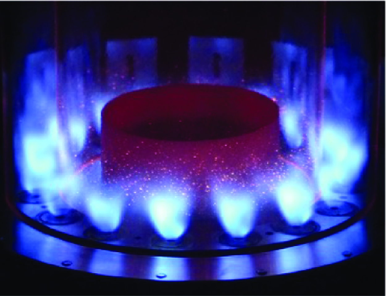
. An array of 8 photomultipliers equipped with an OH* filter centred at 310 nm records the light emitted by eight adjacent flames (see figure 1
b). A mask is placed in front of each flame to ensure that each PM only records the light emitted by one flame. A cylindrical mask is also placed inside the inner cylindrical quartz to hide the flames in the background, as can be seen in figure 1(c), showing the MICCA combustor under operation.
$f_s=32\,768\,\textrm{Hz}$
. An array of 8 photomultipliers equipped with an OH* filter centred at 310 nm records the light emitted by eight adjacent flames (see figure 1
b). A mask is placed in front of each flame to ensure that each PM only records the light emitted by one flame. A cylindrical mask is also placed inside the inner cylindrical quartz to hide the flames in the background, as can be seen in figure 1(c), showing the MICCA combustor under operation.
Table 1. Injectors’ characteristics: swirl number (
 $S_N$
), pressure drop (
$S_N$
), pressure drop (
 $\Delta p$
) and pressure drop coefficient (
$\Delta p$
) and pressure drop coefficient (
 $\sigma$
), obtained from measurements under cold flow conditions for an air mass flow rate of 2.3 g s
$\sigma$
), obtained from measurements under cold flow conditions for an air mass flow rate of 2.3 g s
 $^{-1}$
(Vignat et al. Reference Vignat, Rajendram Soundararajan, Durox, Vié, Renaud and Candel2021).
$^{-1}$
(Vignat et al. Reference Vignat, Rajendram Soundararajan, Durox, Vié, Renaud and Candel2021).


Figure 1. (a) The MICCA annular combustor with an array of eight photomultipliers. (b) Microphones (labelled ‘MX’) and photomultiplier positions (labelled ‘PMX’). (c) View of the MICCA combustor under operation.

Figure 2. Exploded view of an injection unit, showing its main components (a). A top view of the swirler appears in (b).
The injectors, for which an exploded view is presented in figure 2(a), comprise four main elements: an air distributor, an atomizer, a swirler and a terminal plate. Changing the swirler (tangential channels’ radius and orientation figure 2 b) modifies the pressure drop and the swirl number of the units. Two types of injectors are used in this work: a low-swirl low-pressure drop and a high-swirl high-pressure drop, designated respectively as ‘injector S’ and ‘injector U’. The characteristics of the two injectors are gathered in table 1. Additional information on the dynamics of the flames formed by these two injectors is given by Rajendram Soundararajan et al. (Reference Rajendram Soundararajan, Durox, Renaud, Vignat and Candel2022b ) and Latour et al. (Reference Latour, Durox, Renaud and Candel2024a ).
In the present study, the annular combustor is operated at a thermal power
 $\mathcal {P}=118\,\textrm{kW}$
and a global equivalence ratio
$\mathcal {P}=118\,\textrm{kW}$
and a global equivalence ratio
 $\phi =0.9$
. Under these operating conditions, MICCA is stable when equipped with S-injectors and unstable when 16 U-injectors are mounted on the backplane.
$\phi =0.9$
. Under these operating conditions, MICCA is stable when equipped with S-injectors and unstable when 16 U-injectors are mounted on the backplane.
2.2. Modal structure and oscillation frequency
An acoustic analysis of the MICCA combustor has to be carried out to identify the eigenmodes susceptible to being involved in the combustion/acoustics coupling. As discussed in Latour et al. (Reference Latour, Durox, Renaud and Candel2024a ), the combustion chamber in MICCA is decoupled from the plenum by the injectors that are weakly transparent to acoustic waves and introduce an important area change between the chamber and the plenum. The coupling of the injector ports’ acoustics with the combustion chamber acoustics can also be neglected, as shown in the acoustic analysis of MICCA presented in the supplementary material avilable at https://doi.org/10.1017/jfm.2025.10. One can hence assume that the modes that need to be considered are those of the chamber, where the backplane can be assimilated to a rigid wall and the outlet can be modelled as being open to the atmosphere. Experiments indicate that the first azimuthal–first longitudinal (1A1L) mode is involved in the combustion/acoustics coupling in MICCA (Latour et al. Reference Latour, Durox, Renaud and Candel2024a ). Neglecting the radial dependence, the pressure field can then be cast in the form
 \begin{equation} p(x, \theta ,t)_{1A1L} = [A_+\exp (i \theta -i \omega t +i\phi _+) +A_- \exp (-i \theta -i \omega t+i\phi _-)] \psi _{1L}(x) ,\end{equation}
where
 $A_+ \exp (i\phi _+)$
and
$A_+ \exp (i\phi _+)$
and
 $A_- \exp (i\phi _-)$
correspond to the complex amplitudes of the CCW and CW spinning waves respectively,
$A_- \exp (i\phi _-)$
correspond to the complex amplitudes of the CCW and CW spinning waves respectively,
 $\theta$
designates the azimuthal coordinate considered positive in the CCW direction and
$\theta$
designates the azimuthal coordinate considered positive in the CCW direction and
 $\omega$
is the angular frequency. In the previous expression,
$\omega$
is the angular frequency. In the previous expression,
 $\psi _{1L}(x)=\cos [\pi x/(2l^{\prime})]$
is the axial wave function satisfying the boundary conditions on the chamber backplane and at its exhaust, with
$\psi _{1L}(x)=\cos [\pi x/(2l^{\prime})]$
is the axial wave function satisfying the boundary conditions on the chamber backplane and at its exhaust, with
 $l^{\prime}=l+\delta _a$
,
$l^{\prime}=l+\delta _a$
,
 $l$
being the chamber length and
$l$
being the chamber length and
 $\delta _a$
the end correction. For MICCA, pressure measurements near the chamber exhaust indicate that
$\delta _a$
the end correction. For MICCA, pressure measurements near the chamber exhaust indicate that
 $\delta _a \simeq 0.044\,\textrm{m}$
so that
$\delta _a \simeq 0.044\,\textrm{m}$
so that
 $l^{\prime}\simeq 0.44\,\textrm{m}$
(Laera et al. Reference Laera, Prieur, Durox, Schuller, Camporeale and Candel2017).
$l^{\prime}\simeq 0.44\,\textrm{m}$
(Laera et al. Reference Laera, Prieur, Durox, Schuller, Camporeale and Candel2017).
The eigenfrequency corresponding to the 1A1L mode is
 \begin{equation} f_{1A1L}= \left[ \left(\frac {c}{\mathcal {P}_a}\right)^2+ \left(\frac {c}{4l^{\prime}}\right)^2 \right]^{1/2} ,\end{equation}
where
 $\mathcal {P}_a= 2 \pi R$
is the mean perimeter of the system and
$\mathcal {P}_a= 2 \pi R$
is the mean perimeter of the system and
 $c$
the speed of sound. In the MICCA experiments, the perimeter is
$c$
the speed of sound. In the MICCA experiments, the perimeter is
 $\mathcal {P}_a \simeq 1.1\,\textrm{m}$
. Assuming an average temperature in the chamber of
$\mathcal {P}_a \simeq 1.1\,\textrm{m}$
. Assuming an average temperature in the chamber of
 $T\simeq 1400\,\textrm{K}$
(estimated from exhaust gas temperature measurements carried out by Vignat (Reference Vignat2020) with a thermocouple in the single-sector counterpart of the MICCA annular set-up), defining a speed of sound
$T\simeq 1400\,\textrm{K}$
(estimated from exhaust gas temperature measurements carried out by Vignat (Reference Vignat2020) with a thermocouple in the single-sector counterpart of the MICCA annular set-up), defining a speed of sound
 $c=754\,\textrm{m}\,\textrm{s}^-{^1}$
, the eigenfrequency of the 1A1L mode is
$c=754\,\textrm{m}\,\textrm{s}^-{^1}$
, the eigenfrequency of the 1A1L mode is
 $f_{1A1L}\simeq 808\,\textrm{Hz}$
.
$f_{1A1L}\simeq 808\,\textrm{Hz}$
.
The complex wave amplitudes
 $A_+ \exp (i\phi _+)$
and
$A_+ \exp (i\phi _+)$
and
 $A_- \exp (i\phi _-)$
may be retrieved from the eight microphone signals by solving an over-determined system of linear equations using a least squares algorithm. One may then deduce the instability amplitude, defined as
$A_- \exp (i\phi _-)$
may be retrieved from the eight microphone signals by solving an over-determined system of linear equations using a least squares algorithm. One may then deduce the instability amplitude, defined as
 \begin{equation} A = \big[{A_+^2+A_-^2 }\big]^{1/2} .\end{equation}
It is worth noting that
 $A$
is equal to the quaternion formulation amplitude divided by
$A$
is equal to the quaternion formulation amplitude divided by
 $\sqrt 2$
. Finally, the frequency of the instability,
$\sqrt 2$
. Finally, the frequency of the instability,
 $f$
, is experimentally determined from the power spectral density of the pressure signals, calculated using Welch’s method applied to 63 blocks of 8192 samples and a Hamming window weighting with a 50 % overlap. The frequency resolution for these conditions is
$f$
, is experimentally determined from the power spectral density of the pressure signals, calculated using Welch’s method applied to 63 blocks of 8192 samples and a Hamming window weighting with a 50 % overlap. The frequency resolution for these conditions is
 $\Delta f = 4\,\textrm{Hz}$
.
$\Delta f = 4\,\textrm{Hz}$
.
At this point it is worth recalling that the frequency of oscillation of a thermoacoustic system (‘closed-loop’ case) is close to the eigenfrequency of the mode (the ‘open-loop’ frequency) but does not coincide with it because of the shift introduced by the presence of the flames. This shift depends on the flame dynamical characteristics (FDF) and on the set of parameters that also govern the growth rate (Schuller et al. Reference Schuller, Poinsot and Candel2020). One may show (see Schuller et al. Reference Schuller, Poinsot and Candel2020 or § 4) that the relative frequency shift,
 $\Delta \omega / \omega _0$
, is linked to the growth rate,
$\Delta \omega / \omega _0$
, is linked to the growth rate,
 $\omega _i$
, by
$\omega _i$
, by
 $\Delta \omega / \omega _0 \simeq - (\omega _i / \omega _0) \tan \varphi _p$
, where
$\Delta \omega / \omega _0 \simeq - (\omega _i / \omega _0) \tan \varphi _p$
, where
 $\varphi _p$
represents the phase between the pressure and the HRR signals. Since
$\varphi _p$
represents the phase between the pressure and the HRR signals. Since
 $\omega _i / \omega _0\lt 1$
and
$\omega _i / \omega _0\lt 1$
and
 $ \varphi _p \simeq 0$
in an unstable situation, one deduces that
$ \varphi _p \simeq 0$
in an unstable situation, one deduces that
 $|\Delta \omega / \omega _0| \lt \lt 1$
. The previous argument indicates why the shift in frequency is in most cases below 5 % of the modal eigenfrequency, as can be seen in the data compiled by Ghirardo et al. (Reference Ghirardo, Juniper and Bothien2018) or in figures showing the evolution of thermoacoustic systems in the frequency/growth rate plane reported by Noiray et al. (Reference Noiray, Durox, Schuller and Candel2008), Paliès et al. (Reference Paliès, Durox, Schuller and Candel2011) and Laera et al. (Reference Laera, Prieur, Durox, Schuller, Camporeale and Candel2017) and confirmed by experimental results obtained in MICCA (Rajendram Soundararajan et al. Reference Rajendram Soundararajan, Durox, Renaud, Vignat and Candel2022b
; Latour et al. Reference Latour, Durox, Renaud and Candel2024a
).
$|\Delta \omega / \omega _0| \lt \lt 1$
. The previous argument indicates why the shift in frequency is in most cases below 5 % of the modal eigenfrequency, as can be seen in the data compiled by Ghirardo et al. (Reference Ghirardo, Juniper and Bothien2018) or in figures showing the evolution of thermoacoustic systems in the frequency/growth rate plane reported by Noiray et al. (Reference Noiray, Durox, Schuller and Candel2008), Paliès et al. (Reference Paliès, Durox, Schuller and Candel2011) and Laera et al. (Reference Laera, Prieur, Durox, Schuller, Camporeale and Candel2017) and confirmed by experimental results obtained in MICCA (Rajendram Soundararajan et al. Reference Rajendram Soundararajan, Durox, Renaud, Vignat and Candel2022b
; Latour et al. Reference Latour, Durox, Renaud and Candel2024a
).
As pointed out by one reviewer, other aspects of the system, like the temperature distribution linked to the presence of the flames, may also intervene, and affect the modal structure of the azimuthal mode, a phenomenon not accounted for in (2.2), used to determine the frequency of the 1A1L mode of the combustion chamber in MICCA. The temperature distribution can, for example, be easily taken into account by making use of a Helmholtz solver to obtain the modal distributions and eigenfrequencies, as done in previous works (Bourgouin et al. Reference Bourgouin, Durox, Moeck, Schuller and Candel2013; Laera et al. Reference Laera, Prieur, Durox, Schuller, Camporeale and Candel2017). It was found that the obtained eigenfrequencies were not very different from those calculated using theoretical expressions if the mean speed of sound
 $c$
, and hence the temperature in the combustion chamber, are suitably determined, for example, from exhaust gas temperature measurements, as proposed in this work from results reported by Vignat (Reference Vignat2020). The shift in frequency being estimated to be less than a few per cent of the open-loop frequency (obtained from self-sustained oscillation measurements in MICCA), and the calculated value of the open-loop frequency (808 Hz) from the burnt gas temperature estimate falling in the range of frequencies corresponding to observed oscillations (around 800 Hz), one can have confidence in the estimated value. It is, however, interesting to determine the effect of an error in the estimation of the temperature on the calculated frequency of oscillation. To that end, one may consider, for instance, an error
$c$
, and hence the temperature in the combustion chamber, are suitably determined, for example, from exhaust gas temperature measurements, as proposed in this work from results reported by Vignat (Reference Vignat2020). The shift in frequency being estimated to be less than a few per cent of the open-loop frequency (obtained from self-sustained oscillation measurements in MICCA), and the calculated value of the open-loop frequency (808 Hz) from the burnt gas temperature estimate falling in the range of frequencies corresponding to observed oscillations (around 800 Hz), one can have confidence in the estimated value. It is, however, interesting to determine the effect of an error in the estimation of the temperature on the calculated frequency of oscillation. To that end, one may consider, for instance, an error
 $\Delta T= 100\,\textrm{K}$
. The variation in modal frequency is then given by
$\Delta T= 100\,\textrm{K}$
. The variation in modal frequency is then given by
 $\Delta f/f \simeq \Delta c/c = (1/2) \Delta T/ T$
. Taking
$\Delta f/f \simeq \Delta c/c = (1/2) \Delta T/ T$
. Taking
 $T= 1400\,\textrm{K}$
, one finds that
$T= 1400\,\textrm{K}$
, one finds that
 $\Delta f/ f \simeq 3.5\, \%$
and for a frequency
$\Delta f/ f \simeq 3.5\, \%$
and for a frequency
 $f=800\,\textrm{Hz}$
this would induce a variation
$f=800\,\textrm{Hz}$
this would induce a variation
 $\Delta f \simeq 28\,\textrm{Hz}$
.
$\Delta f \simeq 28\,\textrm{Hz}$
.
3. Pressure-based FDF measurements in MICCA
MICCA is now used to collect experimental data on the flames’ HRR responses to pressure oscillations of various amplitudes, which will be presented in the form of a describing function, expressed in the frequency domain. Mixing U- and S-injectors enables us to control the level of limit-cycle pressure fluctuations and favour a standing mode with a fixed nodal line position, as described in Latour et al. (Reference Latour, Durox, Renaud and Candel2024a ). Simultaneous pressure and photomultiplier recordings at different flame positions with respect to the nodal line location may then be used to determine a ‘pressure-based FDF’ (Alhaffar et al. Reference Alhaffar, Latour, Patat, Durox, Renaud, Blaisot, Candel and Baillot2024), defined as
 \begin{equation} \mathcal {F}_p(f, \Pi _j)=\frac {{\widehat {\dot Q}_j}/\overline {\dot Q}}{{\widehat p_j}/{\rho U_b^2}}= G_p(f,\Pi _j)e^{i\varphi (f,\Pi _j)} , \end{equation}
where the index
 $j$
designates the flame number,
$j$
designates the flame number,
 $f$
the frequency,
$f$
the frequency,
 ${\widehat {\dot Q}_j}/\overline {\dot Q}$
the relative HRR fluctuations and
${\widehat {\dot Q}_j}/\overline {\dot Q}$
the relative HRR fluctuations and
 ${\widehat p_j}/{\rho U_b^2}$
the dimensionless pressure fluctuations. The reduced amplitude of the pressure fluctuations at the position of the
${\widehat p_j}/{\rho U_b^2}$
the dimensionless pressure fluctuations. The reduced amplitude of the pressure fluctuations at the position of the
 $j$
th flame is defined by
$j$
th flame is defined by
 $\Pi _j= {(p_{rms})_j}/{(\rho U_b^2)}$
, with
$\Pi _j= {(p_{rms})_j}/{(\rho U_b^2)}$
, with
 $\rho$
the density, taken at the fresh gas temperature, and
$\rho$
the density, taken at the fresh gas temperature, and
 $U_b$
the bulk velocity at the injector outlet, equal to 46 m s
$U_b$
the bulk velocity at the injector outlet, equal to 46 m s
 $^{-1}$
for the investigated operating conditions. It is worth mentioning that the pressure-based FDF defined in this way may be linked to the velocity-based FDF, commonly determined in thermoacoustic investigations (see, for example, Noiray et al. Reference Noiray, Durox, Schuller and Candel2008), through an effective impedance, as discussed in Appendix A.
$^{-1}$
for the investigated operating conditions. It is worth mentioning that the pressure-based FDF defined in this way may be linked to the velocity-based FDF, commonly determined in thermoacoustic investigations (see, for example, Noiray et al. Reference Noiray, Durox, Schuller and Candel2008), through an effective impedance, as discussed in Appendix A.

Figure 3. Staging configurations used for pressure-based FDF measurements showing the placement of the injectors U and S and the photomultiplier positions. The nodal lines observed experimentally are represented by black solid lines.
Seven staging patterns, shown in figure 3, are used for the pressure-based FDF measurements. These injector configurations were selected because they lead to a well-defined standing mode with a controlled nodal line position (Latour et al. Reference Latour, Durox, Renaud and Candel2024a ,Reference Latour, Durox, Renaud and Candel b ) and pressure fluctuation levels enabling a good signal-to-noise ratio for the pressure and photomultiplier recordings. The self-sustained oscillation amplitudes obtained in this way vary between 300 and 1400 Pa, and the instability frequencies lie in the [774, 802] Hz range. Additional information on the determination of pressure-based FDFs can be found in Alhaffar et al. (Reference Alhaffar, Latour, Patat, Durox, Renaud, Blaisot, Candel and Baillot2024), together with a comparison with data from experiments on a linear array of injectors modulated in the transverse direction.
At this point, it is important to stress that, contrary to an externally forced situation, the procedure used in this work to collect the pressure-based FDF data relies on the ability to obtain self-sustained oscillations in MICCA with a well-defined standing mode. The modulation frequency defining flame oscillations in each staging configuration hence results from the closed-loop interaction between the acoustics of the MICCA combustor and the flames, and is therefore dependent on the staging pattern. As discussed in Alhaffar et al. (Reference Alhaffar, Latour, Patat, Durox, Renaud, Blaisot, Candel and Baillot2024), the self-sustained oscillation frequencies of the seven staging patterns used for pressure-based FDF determination vary between 774 and 802 Hz. Although this range of frequency variation is limited, one needs to check that these changes in self-sustained oscillation frequencies do not lead to differences in the flame response. This is done in the supplementary material, where the FDF data points are coloured by the frequency value. There is no visible trend with respect to the relatively small frequency variations and one may conclude that the frequency differences between the staging patterns do not affect the collected pressure-based data.
As also pointed out by a reviewer, flame dynamics data are usually presented as a function of the frequency but this is not the case here. Indeed, in the modelling framework adopted in this work, it is admitted that the frequency of interest is that of the eigenmode involved in the combustion/acoustic coupling and that only the dynamics around the 1A1L eigenfrequency is of interest. This is why flame dynamics data are presented at this frequency only, as in the other investigations of this kind (Ghirardo et al. 2016, 2018, Reference Ghirardo, Nygård, Cuquel and Worth2021).

Figure 4. Pressure-based FDF gain (a,b) and phase (c,d) as a function of
 $\Pi$
for injectors U (a,c) and S (b,d). The colours correspond to the ‘PAN’, ‘IAN’ and ‘VAN’ regions, as defined in (e).
$\Pi$
for injectors U (a,c) and S (b,d). The colours correspond to the ‘PAN’, ‘IAN’ and ‘VAN’ regions, as defined in (e).
The pressure-based FDF gains and phases are plotted as a function of the reduced amplitude of pressure fluctuations,
 $\Pi$
, in figure 4 for injectors U (figure 4
a,c) and S (figure 4
b,d). For the interpretation of the results, the points are labelled ‘PAN’ (pressure anti-node), ‘IAN’ (intensity anti-node) and ‘VAN’ (velocity anti-node), depending on their position with respect to the nodal line location, as defined in Alhaffar et al. (Reference Alhaffar, Latour, Patat, Durox, Renaud, Blaisot, Candel and Baillot2024) and shown in figure 4(e). The data obtained for flames established at various positions with respect to the nodal line indicate that the flame location does not significantly influence its response. The corresponding FDF data points follow nearly similar trends and may be treated independently of their position with respect to the nodal line. The gain values for injector U are higher than those pertaining to injector S, while the phases are close to 0 for the two injectors. For both injectors, the decrease in the gain of the pressure-based FDF with the local pressure amplitude
$\Pi$
, in figure 4 for injectors U (figure 4
a,c) and S (figure 4
b,d). For the interpretation of the results, the points are labelled ‘PAN’ (pressure anti-node), ‘IAN’ (intensity anti-node) and ‘VAN’ (velocity anti-node), depending on their position with respect to the nodal line location, as defined in Alhaffar et al. (Reference Alhaffar, Latour, Patat, Durox, Renaud, Blaisot, Candel and Baillot2024) and shown in figure 4(e). The data obtained for flames established at various positions with respect to the nodal line indicate that the flame location does not significantly influence its response. The corresponding FDF data points follow nearly similar trends and may be treated independently of their position with respect to the nodal line. The gain values for injector U are higher than those pertaining to injector S, while the phases are close to 0 for the two injectors. For both injectors, the decrease in the gain of the pressure-based FDF with the local pressure amplitude
 $\Pi$
, corresponding to flame saturation, follows a nearly linear trend of the form:
$\Pi$
, corresponding to flame saturation, follows a nearly linear trend of the form:
 $G_p=\beta -\kappa \Pi$
. At this point, it is worth noting that
$G_p=\beta -\kappa \Pi$
. At this point, it is worth noting that
 $\beta$
and
$\beta$
and
 $\kappa$
defining the linear and saturation coefficients are dimensionless quantities which differ from the dimensional coefficients used in the cubic formulation of Noiray et al. (Reference Noiray, Bothien and Schuermans2011). The coefficients
$\kappa$
defining the linear and saturation coefficients are dimensionless quantities which differ from the dimensional coefficients used in the cubic formulation of Noiray et al. (Reference Noiray, Bothien and Schuermans2011). The coefficients
 $\beta$
and
$\beta$
and
 $\kappa$
, that are here deduced from a least squares regression for the two injectors U and S, define the linear models superimposed on the data points in figure 4.
$\kappa$
, that are here deduced from a least squares regression for the two injectors U and S, define the linear models superimposed on the data points in figure 4.
As indicated by a reviewer, other expressions, such as higher-order polynomial functions, could be used to fit the experimental FDF data. It is found, however, that the
 $R^2$
statistical index is only slightly improved when using second-order or cubic polynomials as it changes from 0.69 to 0.74 for injector U. However, by using higher-order fits (cubic or fourth-order polynomials), one runs the risk of over-fitting, and some points, which appear like ‘outliers’, may weigh in the fit although they should not. This is why the linear fit is a good compromise in terms of data representation and ease of insertion in an analytical formulation. This is confirmed in the sensitivity analysis carried out in § 5.6 for the linear and quadratic fits where one examines effects of errors in the fitting on the predicted limit-cycle oscillation amplitudes.
$R^2$
statistical index is only slightly improved when using second-order or cubic polynomials as it changes from 0.69 to 0.74 for injector U. However, by using higher-order fits (cubic or fourth-order polynomials), one runs the risk of over-fitting, and some points, which appear like ‘outliers’, may weigh in the fit although they should not. This is why the linear fit is a good compromise in terms of data representation and ease of insertion in an analytical formulation. This is confirmed in the sensitivity analysis carried out in § 5.6 for the linear and quadratic fits where one examines effects of errors in the fitting on the predicted limit-cycle oscillation amplitudes.
To finish, the relatively large dispersion in the FDF gain and phase values observed for injector S is due to a higher uncertainty in the measurements, since S-injectors are mainly located close to the pressure nodal line where pressure fluctuations are low. This might also be linked to differences between injectors, as reported by Nygård, Ghirardo & Worth (2021), where different responses were observed for flames submitted to a spinning mode and interpreted as resulting from small symmetry-breaking effects.
4. Investigation of two heat release rate formulations
Before using the pressure-based FDFs obtained in § 3 in an analytical framework (§ 5), two HRR formulations are examined in a simplified framework to investigate the impact of the flame response model on the slow-flow variables’ dynamics: the first is the cubic polynomial formulation, introduced by Noiray et al. (Reference Noiray, Bothien and Schuermans2011),
 ${\dot Q}^{\prime}= \beta ^* p- \kappa _1^* p^3$
, and the second is of the form
${\dot Q}^{\prime}= \beta ^* p- \kappa _1^* p^3$
, and the second is of the form
 ${\dot Q}^{\prime}=g^*(a) p$
, where the saturation process is a function
${\dot Q}^{\prime}=g^*(a) p$
, where the saturation process is a function
 $g^*$
of the slowly varying instability amplitude
$g^*$
of the slowly varying instability amplitude
 $a$
of the form
$a$
of the form
 $g^*(a)=\beta ^*-\kappa _2^* a$
, as observed in the experimental data reported in § 3. In the two models investigated, the saturation coefficients will be denoted
$g^*(a)=\beta ^*-\kappa _2^* a$
, as observed in the experimental data reported in § 3. In the two models investigated, the saturation coefficients will be denoted
 $\kappa _1^*$
and
$\kappa _1^*$
and
 $\kappa _2^*$
, and since they intervene in different formulations, their dimensions and values are also different.
$\kappa _2^*$
, and since they intervene in different formulations, their dimensions and values are also different.
For simplicity, a single oscillator model is considered in this section. Physically, this situation corresponds, for example, to a thermoacoustic system with a self-sustained longitudinal oscillation. The case of azimuthal modes in an annular system will be considered in § 5.
4.1.
Polynomial heat release rate fluctuation formulation:
 ${\dot Q}^{\prime}= \beta ^* p- \kappa _1^* p^3$

The starting point is the non-homogeneous wave equation, derived from the combination of the mass, momentum and energy equations for low-Mach flows and perfect gases, to which a damping term is added in the form
 $\alpha ({\partial p}/{\partial t})$
to account for the losses in the system
$\alpha ({\partial p}/{\partial t})$
to account for the losses in the system
 \begin{equation} \frac {\partial ^2 p}{\partial t^2}-\rho c^2 \boldsymbol {\nabla } \boldsymbol {\cdot } \frac {1}{\rho }\boldsymbol {\nabla } p =(\gamma -1) \frac {\partial {\dot q}^{\prime}}{\partial t} -\alpha \frac {\partial p}{\partial t} .\end{equation}
In this expression,
 ${\dot q}^{\prime}$
,
${\dot q}^{\prime}$
,
 $\rho$
,
$\rho$
,
 $c$
and
$c$
and
 $\gamma$
respectively designate the volumetric HRR fluctuations, the mean density, the mean speed of sound and the specific heat ratio. The steps leading to the derivation of (4.1) are recalled, for instance, in Nicoud et al. (Reference Nicoud, Benoit, Sensiau and Poinsot2007, Reference Noiray, Bothien and Schuermans2011) or Ghirardo et al. (Reference Ghirardo, Boudy and Bothien2018).
$\gamma$
respectively designate the volumetric HRR fluctuations, the mean density, the mean speed of sound and the specific heat ratio. The steps leading to the derivation of (4.1) are recalled, for instance, in Nicoud et al. (Reference Nicoud, Benoit, Sensiau and Poinsot2007, Reference Noiray, Bothien and Schuermans2011) or Ghirardo et al. (Reference Ghirardo, Boudy and Bothien2018).
At this stage, it is interesting to discuss the zero-Mach-number assumption used to write (4.1), which is common to most thermoacoustic investigations of annular systems (Nicoud et al. Reference Nicoud, Benoit, Sensiau and Poinsot2007, Reference Noiray, Bothien and Schuermans2011; Ghirardo et al. Reference Ghirardo, Juniper and Moeck2016). In annular combustors that are typically used in gas turbines, the Mach number is low to ensure that the residence time of reactants is sufficient for flame stabilization, to allow complete conversion into products and minimize pressure losses associated with heat addition. The analysis by Nicoud et al. (Reference Nicoud, Benoit, Sensiau and Poinsot2007) indicates that the mean flow terms can be neglected if the characteristic Mach number is small compared with the ratio of the flame dimension to the typical acoustic wavelength and this condition is generally fulfilled. There are, however, some more subtle effects of the presence of a mean swirling flow on the acoustic modes in an annular system. If, for example, the azimuthal velocity is high enough, the global rotation of the flow will suppress the degeneracy of the azimuthal modes and the CW and CCW modes will feature different eigenfrequencies and growth rates (Bauerheim, Cazalens & Poinsot Reference Bauerheim, Cazalens and Poinsot2015). It is also indicated by Faure-Beaulieu et al. (Reference Faure-Beaulieu, Pedergnana and Noiray2023) that, when a swirl is imposed in a certain direction, a statistical preference is observed toward mixed states propagating against the swirl. However, in the situation at hand, the global rotation velocity is so small that the two eigenfrequencies cannot be distinguished in the spectral analysis of the microphone signals and the statistical preference is expected to be small compared with the symmetry-breaking effects induced by injector staging of the kind investigated in the present work.
A second assumption made in writing (4.1) is that the acoustics may be treated as a linear process. This is also widely adopted because the levels of relative pressure fluctuations in typical gas turbine combustion systems remain below a few per cent of the chamber pressure, in contrast with rocket thrust chambers where relative fluctuation levels may reach up to 40 % of the chamber pressure. The reader can find further details on the nonlinear acoustics in rocket engines in Culick (Reference Culick1994). In the case of gas turbines, the level of oscillation does not exceed a few per cent. In the MICCA experimental set-up, even at a pressure fluctuations level of 5000 Pa (5 % of the chamber pressure), the microphone signals remain sinusoidal while the light intensity signal from OH
 $^*$
radicals detected by photomultipliers facing the flames become highly nonlinear (Prieur et al. Reference Prieur, Durox, Schuller and Candel2018). One may then safely assume that the acoustics is linear and that the main source of nonlinearity in the system is linked to the unsteady HRRs and that this nonlinearity can be represented with a FDF (Dowling Reference Dowling1997; Noiray et al. Reference Noiray, Durox, Schuller and Candel2008).
$^*$
radicals detected by photomultipliers facing the flames become highly nonlinear (Prieur et al. Reference Prieur, Durox, Schuller and Candel2018). One may then safely assume that the acoustics is linear and that the main source of nonlinearity in the system is linked to the unsteady HRRs and that this nonlinearity can be represented with a FDF (Dowling Reference Dowling1997; Noiray et al. Reference Noiray, Durox, Schuller and Candel2008).
Finally, it is also worth noting that the
 $\alpha$
appearing in this expression corresponds to the damping rate of acoustic energy and is equal to twice the damping rate of pressure. The value of this damping rate can be obtained in various ways using, for instance, system identification methods, as proposed in Boujo et al. (Reference Boujo, Denisov, Schuermans and Noiray2016). Another possibility, used in this study (see § 5), relies on source term measurements at the limit cycle, as exemplified in Durox et al. (Reference Durox, Schuller, Noiray, Birbaud and Candel2009) or Latour et al. (Reference Latour, Durox, Renaud and Candel2024b
), which will be discussed, along with the modelling hypothesis, in § 5.
$\alpha$
appearing in this expression corresponds to the damping rate of acoustic energy and is equal to twice the damping rate of pressure. The value of this damping rate can be obtained in various ways using, for instance, system identification methods, as proposed in Boujo et al. (Reference Boujo, Denisov, Schuermans and Noiray2016). Another possibility, used in this study (see § 5), relies on source term measurements at the limit cycle, as exemplified in Durox et al. (Reference Durox, Schuller, Noiray, Birbaud and Candel2009) or Latour et al. (Reference Latour, Durox, Renaud and Candel2024b
), which will be discussed, along with the modelling hypothesis, in § 5.
In flames that are nearly isobaric, the product
 $\rho c^2$
is nearly constant and may be introduced in the divergence operator in (4.1). One may also assume that the flame is compact with respect to the acoustic wavelength and consider that the HRR fluctuations are concentrated at one point,
$\rho c^2$
is nearly constant and may be introduced in the divergence operator in (4.1). One may also assume that the flame is compact with respect to the acoustic wavelength and consider that the HRR fluctuations are concentrated at one point,
 $\boldsymbol {x}_f$
. One may then write
$\boldsymbol {x}_f$
. One may then write
 ${\dot q}^{\prime}= \delta (\boldsymbol {x}-\boldsymbol {x}_f){\dot Q}^{\prime}$
, where
${\dot q}^{\prime}= \delta (\boldsymbol {x}-\boldsymbol {x}_f){\dot Q}^{\prime}$
, where
 $\delta$
is the Dirac function and
$\delta$
is the Dirac function and
 ${\dot Q}^{\prime}$
corresponds to the HRR fluctuations integrated over the volume of the flame. Hence, the wave equation may now be replaced by
${\dot Q}^{\prime}$
corresponds to the HRR fluctuations integrated over the volume of the flame. Hence, the wave equation may now be replaced by
 \begin{equation} \frac {\partial ^2 p}{\partial t^2}-\boldsymbol {\nabla } \boldsymbol {\cdot } c^2 \boldsymbol {\nabla } p =(\gamma -1) \delta (\boldsymbol {x}-\boldsymbol {x}_f) \frac {\partial {\dot Q}^{\prime}}{\partial t} -\alpha \frac {\partial p}{\partial t} .\end{equation}
The normal modes of this equation, in the absence of heat release and damping, are such that
 \begin{equation} \boldsymbol {\nabla } \boldsymbol {\cdot } c^2 \boldsymbol {\nabla } \psi _n + \omega _n^2 \psi _n=0 ,\end{equation}
where
 $\omega _n$
and
$\omega _n$
and
 $\psi _n$
represent the modal eigenvalues and eigenfunctions, respectively. The pressure field can then be expanded on the orthogonal basis formed by the eigenmodes
$\psi _n$
represent the modal eigenvalues and eigenfunctions, respectively. The pressure field can then be expanded on the orthogonal basis formed by the eigenmodes
 $\psi _n$
, solutions of the homogeneous wave equation
$\psi _n$
, solutions of the homogeneous wave equation
 \begin{equation} p=\sum _n \eta _n(t) \psi _n(\boldsymbol {x}) ,\end{equation}
where
 $\eta _n$
represents the amplitude of the nth mode. For homogeneous boundary conditions, the normal modes
$\eta _n$
represents the amplitude of the nth mode. For homogeneous boundary conditions, the normal modes
 $\psi _n$
are orthogonal (see for example Nicoud et al. Reference Nicoud, Benoit, Sensiau and Poinsot2007) and one may write
$\psi _n$
are orthogonal (see for example Nicoud et al. Reference Nicoud, Benoit, Sensiau and Poinsot2007) and one may write
 \begin{equation} \int _V \psi _n \psi _m \textrm{d}V= \Lambda _n \delta _{mn} \, \, \textrm {with} \,\, \delta _{nn}= 1 \,\, \textrm { and } \,\, \delta _{mn}= 0 \,\, \textrm {when} \,\, m \ne n .\end{equation}
Introducing the modal expansion (4.4) in the wave equation (4.2) and projecting the result on the normal modes, one obtains a set of differential equations for the modal amplitudes
 $\eta _n(t)$
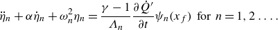 \begin{equation} {\ddot \eta _n}+ \alpha {\dot \eta _n} + \omega _n^2 \eta _n = \frac {\gamma -1}{\Lambda _n} \frac {\partial {\dot Q}^{\prime}}{\partial t} \psi _n(x_f) \,\, \textrm {for} \,\, n=1,2\ldots .\end{equation}
For the sake of simplicity, it will be assumed in what follows that a single mode, characterized by an eigenfrequency
 $\omega _0$
and a modal amplitude
$\omega _0$
and a modal amplitude
 $\eta$
, is involved in the combustion/acoustics coupling. This situation physically corresponds, for instance, to a coupling by a longitudinal mode in a single-injector set-up. This assumption is made to analyse the effects of the HRR formulation in the simplest possible framework. In this case, the pressure field reads
$\eta$
, is involved in the combustion/acoustics coupling. This situation physically corresponds, for instance, to a coupling by a longitudinal mode in a single-injector set-up. This assumption is made to analyse the effects of the HRR formulation in the simplest possible framework. In this case, the pressure field reads
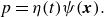 \begin{equation} p=\eta (t) \psi (\boldsymbol {x}) .\end{equation}
One possibility, introduced by Noiray et al. (Reference Noiray, Bothien and Schuermans2011), consists in writing
 ${\dot Q}^{\prime}$
in the form of a third-order polynomial of the pressure
${\dot Q}^{\prime}$
in the form of a third-order polynomial of the pressure
 ${\dot Q}^{\prime}=\beta ^* p-\kappa ^*p^3$
, which, using (4.7), reads
${\dot Q}^{\prime}=\beta ^* p-\kappa ^*p^3$
, which, using (4.7), reads
 \begin{equation} {\dot Q}^{\prime}= \beta ^*\eta \psi _f- \kappa _1^* \eta ^3 \psi _f^3 ,\end{equation}
where
 $\psi _f= \psi ({\boldsymbol x}_f)$
. It is then convenient to define
$\psi _f= \psi ({\boldsymbol x}_f)$
. It is then convenient to define
 \begin{equation} \beta = [(\gamma -1)/\Lambda ] \beta ^* \psi _f^2 \quad \textrm {and} \quad \kappa _1= [(\gamma -1)/\Lambda ] \kappa _1^* \psi _f^4 .\end{equation}
With these notations, the dynamical equation governing
 $\eta$
becomes
$\eta$
becomes
 \begin{equation} {\ddot \eta }+ \alpha {\dot \eta } + \omega _0^2 \eta =\beta {\dot \eta } - 3{\kappa _1} \eta ^2 {\dot \eta }.\end{equation}
In this expression,
 $\beta$
is the linear rate of growth corresponding to small pressure perturbations and
$\beta$
is the linear rate of growth corresponding to small pressure perturbations and
 $\kappa _1$
is positive and governs the saturation process taking place at large oscillation amplitudes. The damping coefficient
$\kappa _1$
is positive and governs the saturation process taking place at large oscillation amplitudes. The damping coefficient
 $\alpha$
is the rate at which
$\alpha$
is the rate at which
 $\eta ^2$
decays as a function of time when the right-hand side of (4.10) is equal to zero.
$\eta ^2$
decays as a function of time when the right-hand side of (4.10) is equal to zero.
Solutions of this nonlinear differential equation may be obtained by making use of the method of averaging introduced by Krylov & Bogoliubov (Reference Krylov and Bogoliubov1950). This standard method is used here, as in most previous studies on azimuthal combustion instabilities referenced in the introduction. As pointed out by a reviewer, this method may not always yield the best approximation of the slow-flow variables, and other approaches, such as the multiple time scales method, can be used, as exemplified in Sirignano & Krieg (Reference Sirignano and Krieg2016). The reader is also referred to Cole (Reference Cole1968), Nayfeh & Mook (Reference Nayfeh and Mook1979) and Verhulst (Reference Verhulst1996) for additional information and the comparison of different approaches for the obtention of slow-flow variable equations. However, the advantage of the averaging method is that it gives access to the slow-flow variables with a reasonable amount of calculations and is sufficient to reveal the effects of the different HRR formulations.
The averaging method is quite standard, but the main steps are nevertheless provided here to facilitate the understanding of the derivation. The solution is first written in terms of a slowly varying amplitude
 $a$
and a phase
$a$
and a phase
 $\varphi$
 \begin{equation} \eta (t)= a(t) \cos [\omega _0 t + \varphi (t)]. \end{equation}
To introduce this expression in (4.10), one needs to calculate the first derivative of
 $\eta$
 \begin{equation} {\dot \eta }= {\dot a} \cos (\omega _0 t + \varphi )-a \omega _0 \sin (\omega _0 t + \varphi ) - a {\dot \varphi }\sin (\omega _0 t + \varphi ). \end{equation}
In the method of averaging, it is standard to impose at this stage
 \begin{equation} {\dot a} \cos (\omega _0 t + \varphi )- a {\dot \varphi }\sin (\omega _0 t + \varphi )=0 ,\end{equation}
so that
 ${\dot \eta }= - a \omega _0\sin (\omega _0 t + \varphi )$
, and one may then proceed to calculate the second derivative of
${\dot \eta }= - a \omega _0\sin (\omega _0 t + \varphi )$
, and one may then proceed to calculate the second derivative of
 $\eta$
 \begin{equation} {\ddot \eta }=-a \omega _0^2 \cos (\omega _0 t + \varphi )-{\dot a}\omega _0\sin (\omega _0 t + \varphi ) -a\omega _0 {\dot \varphi }\cos (\omega _0 t + \varphi ) .\end{equation}
Inserting the previous expression in (4.10) and noting
 $\phi = \omega _0t +\varphi$
, one obtains, after some straightforward calculations,
$\phi = \omega _0t +\varphi$
, one obtains, after some straightforward calculations,
 \begin{equation} {\dot a}\sin \phi +a {\dot \varphi }\cos \phi =-\alpha a \sin \phi + \beta a \sin \phi - 3 \kappa _1 a^3 \cos ^2 \phi \sin \phi. \end{equation}
This last equation, together with (4.13), form a linear system. The determinant of this system is
 $\Delta =1$
, and it is a simple matter to obtain
$\Delta =1$
, and it is a simple matter to obtain
 \begin{eqnarray} {\dot a}&= -\alpha a \sin ^2 \phi + \beta a \sin ^2 \phi - 3 \kappa _1 a^3 \cos ^2 \phi \sin ^2\phi ,\end{eqnarray}
 \begin{eqnarray} a{\dot \varphi }&=-\alpha a \sin \phi \cos \phi + \beta a \sin \phi \cos \phi - 3 \kappa _1 a^3 \cos ^3 \phi \sin \phi .\end{eqnarray}
These equations may then be averaged over a period of oscillation
 $T= 2 \pi / \omega _0$
by taking into account that
$T= 2 \pi / \omega _0$
by taking into account that
 $a$
and
$a$
and
 $\varphi$
on the right-hand side do not vary over that period. The averages on the left-hand side are
$\varphi$
on the right-hand side do not vary over that period. The averages on the left-hand side are
 $[a(t+T)-a(T)]/T$
and
$[a(t+T)-a(T)]/T$
and
 $[\varphi (t+T)-\varphi (T)]/T$
, which represent the slow variable derivatives with respect to time
$[\varphi (t+T)-\varphi (T)]/T$
, which represent the slow variable derivatives with respect to time
 \begin{align}\frac {\textrm{d}\it a}{\textrm{d}\it t} = [-\alpha /2 + \beta /2 -3 \kappa _1 a^2/ 8]a ,\end{align}
 \begin{align} a \frac {\textrm{d}\varphi }{\textrm{d}\it t} = 0. \end{align}
According to this model, the phase
 $\varphi$
remains constant, while the rate of change of the amplitude
$\varphi$
remains constant, while the rate of change of the amplitude
 $a$
is given by the differential equation (4.18), which may also be written
$a$
is given by the differential equation (4.18), which may also be written
 \begin{equation} \frac {1}{a}\frac {\textrm{d}\it a}{\textrm{d}\it t}= \frac { (\beta - \alpha )}{2} -\frac {3}{8} \kappa _1 a^2 .\end{equation}
When
 $\beta \lt \alpha$
, the right-hand side of this equation is negative and the amplitude decays from its initial value at a rate that is always greater than
$\beta \lt \alpha$
, the right-hand side of this equation is negative and the amplitude decays from its initial value at a rate that is always greater than
 $(\beta - \alpha )/{2}$
. When
$(\beta - \alpha )/{2}$
. When
 $\beta \gt \alpha$
, the previous equation has a stationary solution with a finite amplitude corresponding to a limit cycle
$\beta \gt \alpha$
, the previous equation has a stationary solution with a finite amplitude corresponding to a limit cycle
 \begin{equation} a_s= [(4/3)(\beta -\alpha )/(\kappa _1)]^{1/2} .\end{equation}
This behaviour is typical of a Van der Pol oscillator and one may ask whether the stationary solution is stable. This question can be settled by considering the time evolution of a small perturbation in the amplitude,
 $a=a_s+\epsilon$
. Inserting this expression in the dynamical equation for the amplitude and only retaining first-order terms in
$a=a_s+\epsilon$
. Inserting this expression in the dynamical equation for the amplitude and only retaining first-order terms in
 $\epsilon$
, one obtains, after some straightforward calculations,
$\epsilon$
, one obtains, after some straightforward calculations,
 \begin{equation} \frac {\textrm{d}\epsilon }{\textrm{d}\it t}=-\frac {3}{4}\kappa _1 a_s^2 \epsilon .\end{equation}
The perturbation in amplitude diminishes exponentially if
 $\kappa _1$
is positive and one concludes that the stationary solution corresponds to a stable limit cycle.
$\kappa _1$
is positive and one concludes that the stationary solution corresponds to a stable limit cycle.
If now the flame response is delayed by a time lag
 $\tau _p$
, such that
$\tau _p$
, such that
 ${\dot Q}^{\prime}=\beta ^*p(t-\tau _p)-\kappa ^*p(t-\tau _p)^3$
, one gets the following system for the slow-flow variable equations:
${\dot Q}^{\prime}=\beta ^*p(t-\tau _p)-\kappa ^*p(t-\tau _p)^3$
, one gets the following system for the slow-flow variable equations:
 \begin{align} \frac {1}{a}\frac {\textrm{d}\it a}{\textrm{d}\it t} = -\frac {1}{2}[\alpha - (\beta -3 \kappa _1 a^2/ 4) \cos (\omega _0 \tau _p)] ,\end{align}
 \begin{align} \frac {\textrm{d}\varphi }{\textrm{d}\it t} = -\frac {1}{2}(\beta - 3 \kappa _1 a^2/4) \sin (\omega _0 \tau _p) .\end{align}
Compared with (4.18) and (4.19), one can see that the introduction of a time delay in the flame response induces a drift in the slow-flow variable
 $\varphi$
and modifies the growth rate and the amplitude of the limit cycle.
$\varphi$
and modifies the growth rate and the amplitude of the limit cycle.
However, the problem is that the model used in this section to represent HRR fluctuations as a function of pressure does not allow for an easy and flexible adaptation to experimental flame dynamics data, such as those reported in § 3, figure 4, commonly expressed in terms of FDFs, as a function of slow-flow variables such as the oscillation level. In addition, the amplitude of the stationary solution (4.21) is proportional to the square root of
 $\beta -\alpha$
, and we will see later on (§ 6) that experiments do not comply with this law. For these reason, an alternative HRR model is examined in § 4.2.
$\beta -\alpha$
, and we will see later on (§ 6) that experiments do not comply with this law. For these reason, an alternative HRR model is examined in § 4.2.
4.2.
Heat release rate expressed as a function of the oscillation amplitude:
${\dot Q}^{\prime}= g^*(a)p$

One may now consider a second model that is more flexible and easily adaptable to the experimental data reported in § 3 (figure 4). The choice of this formulation is motivated by the fact that experimental FDF data available in the literature (and used as input in the modelling framework of the kind considered here) are commonly presented as a function of oscillation amplitude level or slow-flow variables (see for instance Ghirardo et al. (Reference Ghirardo, Juniper and Moeck2016) who use experimental FDF data reported as a function of the level of oscillation or Ghirardo et al. (Reference Ghirardo, Nygård, Cuquel and Worth2021) who consider flame response functions expressed in terms of slow-flow variables, like the nature angle,
 $\chi$
). An expression for the HRR as a function of slow-flow variables is better suited for practical applications and corresponds to the natural way of presenting flame dynamics data found in the literature. Investigating this kind of formulation hence enables a simpler comparison between different flame dynamics data.
$\chi$
). An expression for the HRR as a function of slow-flow variables is better suited for practical applications and corresponds to the natural way of presenting flame dynamics data found in the literature. Investigating this kind of formulation hence enables a simpler comparison between different flame dynamics data.
The central idea is that the ratio between the HRR and pressure fluctuations is a function of the oscillation amplitude level
 $g^*(a)$
, so that
$g^*(a)$
, so that
 ${\dot Q}^{\prime}=g^*(a)p$
. Considering, as in § 4.1, a coupling by a single mode of modal amplitude
${\dot Q}^{\prime}=g^*(a)p$
. Considering, as in § 4.1, a coupling by a single mode of modal amplitude
 $\eta$
(
$\eta$
(
 $p=\eta \psi$
), the HRR term reads
$p=\eta \psi$
), the HRR term reads
 \begin{equation} {\dot Q}^{\prime}= g^*(a) \eta \psi _f .\end{equation}
To simplify notations, it is convenient to define
 \begin{equation} g(a)= \frac {\gamma -1}{\Lambda } g^*(a) \psi _f^2 ,\end{equation}
and the dynamical equation for
 $\eta$
now becomes
$\eta$
now becomes
 \begin{equation} {\ddot \eta }+ \alpha {\dot \eta } + \omega _0^2 \eta =g^{\prime}(a){\dot a}\eta + g(a) {\dot \eta } .\end{equation}
Introducing
 $\phi = \omega _0 t + \varphi$
and noting that
$\phi = \omega _0 t + \varphi$
and noting that
 $\dot \eta = -a\omega _0 \sin (\omega _0 t + \varphi )$
, a few calculations yield
$\dot \eta = -a\omega _0 \sin (\omega _0 t + \varphi )$
, a few calculations yield
 \begin{equation} {\dot a}\left[\sin \phi + \frac {g^{\prime}(a)a}{\omega _0}\cos \phi \right] +a {\dot \varphi }\cos \phi = -\alpha a \sin \phi + g(a)a \sin \phi . \end{equation}
The system of equations now reads
 \begin{equation} \begin{bmatrix} \cos \phi & &-\sin \phi \\ \sin \phi +\frac {g^{\prime}(a)a}{\omega _0}\cos \phi & &\cos \phi \end{bmatrix} \begin{bmatrix} {\dot a}\\ a{\dot \varphi } \end{bmatrix} = \begin{bmatrix} 0 \\ -\alpha a \sin \phi + g(a)a \sin \phi \end{bmatrix} ,\end{equation}
and the determinant is
 \begin{equation} \Delta =1 + \frac {g^{\prime}(a)a}{\omega _0} \sin \phi \cos \phi .\end{equation}
System 4.29 may then be solved, yielding
 \begin{align} {\dot a} = \frac {1}{\Delta }[-\alpha a + g(a)a] \sin ^2 \phi ,\end{align}
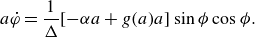 \begin{align} a{\dot \varphi } = \frac {1}{\Delta }[-\alpha a + g(a)a]\sin \phi \cos \phi .\end{align}
Averaging over a period is now complicated because the determinant appears in the denominator but it is possible to make an approximation by considering that
 $g^{\prime}(a)a/\omega _0\lt \lt 1$
(see Appendix B, where the order of magnitude of this term is estimated) and write
$g^{\prime}(a)a/\omega _0\lt \lt 1$
(see Appendix B, where the order of magnitude of this term is estimated) and write
 \begin{align} {1}/{\Delta } \simeq 1- \frac{g^{\prime}(a)a}{\omega _0}\sin \phi \cos \phi. \end{align}
Introducing this expression in (4.31) and (4.32) and integrating over a period yields
 \begin{align} \frac {\textrm{d}\it a}{\textrm{d}\it t} = \frac {1}{2} [-\alpha +g(a)]a ,\end{align}
 \begin{align} \frac {\textrm{d}\varphi }{\textrm{d}\it t} = [-\alpha + g(a)]\frac {[-g^{\prime}(a)a]}{8\omega _0} .\end{align}
These equations indicate that both
 $a$
and
$a$
and
 $\varphi$
slowly vary with time. An example of resolution of (4.27) when
$\varphi$
slowly vary with time. An example of resolution of (4.27) when
 $g(a) = \beta -\kappa _2 a$
is shown in figure 5(a). The envelope is obtained by integrating (4.34) for the slow variable
$g(a) = \beta -\kappa _2 a$
is shown in figure 5(a). The envelope is obtained by integrating (4.34) for the slow variable
 $a$
. A steady solution exists if
$a$
. A steady solution exists if
 $g(a)\gt \alpha$
in an interval of amplitudes and if
$g(a)\gt \alpha$
in an interval of amplitudes and if
 $g(a)-\alpha$
vanishes for an amplitude
$g(a)-\alpha$
vanishes for an amplitude
 $a_s$
. Here again, one may ask whether the stationary solution corresponds to a stable limit cycle. For this, one can consider a small perturbation in amplitude, such that
$a_s$
. Here again, one may ask whether the stationary solution corresponds to a stable limit cycle. For this, one can consider a small perturbation in amplitude, such that
 $a=a_s+ \epsilon$
in the vicinity of the stationary solution (or solutions), defined by
$a=a_s+ \epsilon$
in the vicinity of the stationary solution (or solutions), defined by
 $g(a_s)-\alpha =0$
. Only retaining first-order terms with respect to
$g(a_s)-\alpha =0$
. Only retaining first-order terms with respect to
 $\epsilon$
, one obtains
$\epsilon$
, one obtains
 \begin{equation} \frac {\textrm{d}\epsilon }{\textrm{d}\it t}=\frac {1}{2} g^{\prime}(a_s) a_s \epsilon .\end{equation}
The perturbation vanishes exponentially if
 $g^{\prime}(a_s)\lt 0$
and, in that case, the stationary solution corresponds to a stable limit cycle. However, if
$g^{\prime}(a_s)\lt 0$
and, in that case, the stationary solution corresponds to a stable limit cycle. However, if
 $g^{\prime}(a_s)\gt 0$
, the small perturbation grows exponentially and the stationary solution is unstable.
$g^{\prime}(a_s)\gt 0$
, the small perturbation grows exponentially and the stationary solution is unstable.
To fix the ideas, one may consider the case where
 $g(a)$
is a linearly decreasing function of the amplitude,
$g(a)$
is a linearly decreasing function of the amplitude,
 $f(a)=\beta -\kappa _2 a$
. In that case
$f(a)=\beta -\kappa _2 a$
. In that case
 \begin{align} \frac {\textrm{d}\it a}{\textrm{d}\it t} = \frac {1}{2} ( \beta -\alpha - \kappa _2 a)a ,\end{align}
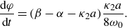 \begin{align} \frac {\textrm{d}\varphi }{\textrm{d}\it t} = ( \beta -\alpha - \kappa _2 a)\frac {\kappa _2 a}{8\omega _0} .\end{align}
If
 $\beta \gt \alpha$
, the stationary solution has an amplitude
$\beta \gt \alpha$
, the stationary solution has an amplitude
 $a_s=(\beta -\alpha )/\kappa _2$
and the rate of change of
$a_s=(\beta -\alpha )/\kappa _2$
and the rate of change of
 $\varphi$
is positive when the amplitude
$\varphi$
is positive when the amplitude
 $a$
is below
$a$
is below
 $a_s$
. This situation corresponds to a positive shift in the frequency of oscillation. We will see later on that the linear relation between
$a_s$
. This situation corresponds to a positive shift in the frequency of oscillation. We will see later on that the linear relation between
 $\beta -\alpha$
and the limit-cycle amplitude deduced in this case, is much closer to what is observed experimentally (see the end of § 6 and Appendix E).
$\beta -\alpha$
and the limit-cycle amplitude deduced in this case, is much closer to what is observed experimentally (see the end of § 6 and Appendix E).

Figure 5. (a) Typical solution of the second-order oscillator (4.27) when
 $g(a) = \beta -\kappa _2 a$
. The envelope is obtained by integrating (4.34) for the slow variable
$g(a) = \beta -\kappa _2 a$
. The envelope is obtained by integrating (4.34) for the slow variable
 $a$
. (b) Limit-cycle oscillation amplitude
$a$
. (b) Limit-cycle oscillation amplitude
 $a_s$
as a function of
$a_s$
as a function of
 $\beta$
for the polynomial HRR formulation (black curve) and the new formulation of the form
$\beta$
for the polynomial HRR formulation (black curve) and the new formulation of the form
 ${\dot Q}^{\prime}= g^*(a)p$
(red curve) for different values of the saturation coefficients
${\dot Q}^{\prime}= g^*(a)p$
(red curve) for different values of the saturation coefficients
 $\kappa _1$
and
$\kappa _1$
and
 $\kappa _2$
. Here,
$\kappa _2$
. Here,
 $\alpha$
designates the damping rate of the system.
$\alpha$
designates the damping rate of the system.
It is also instructive to model the situation where the flame response is delayed by a time lag
 $\tau _p$
, and in this case,
$\tau _p$
, and in this case,
 ${\dot Q}^{\prime}= g^*(a(t-\tau _p)) p(t-\tau _p)$
. Since the order of magnitude of the delay is well below that of a period of oscillation, one may assume that
${\dot Q}^{\prime}= g^*(a(t-\tau _p)) p(t-\tau _p)$
. Since the order of magnitude of the delay is well below that of a period of oscillation, one may assume that
 $a(t-\tau _p) \approx a(t)$
(
$a(t-\tau _p) \approx a(t)$
(
 $a$
is a slow-flow variable assumed constant over a period of oscillation) and write
$a$
is a slow-flow variable assumed constant over a period of oscillation) and write
 ${\dot Q}^{\prime}= g^*(a)p(t-\tau _p)$
. For the pressure field of (4.7), one has
${\dot Q}^{\prime}= g^*(a)p(t-\tau _p)$
. For the pressure field of (4.7), one has
 \begin{equation} {\dot Q}^{\prime}= g^*(a) \eta (t-\tau _p) \psi _f .\end{equation}
Introducing
 $g(a)= [{(\gamma -1)}/{\Lambda }]g^*(a) \psi _f^2$
and applying the method of averaging, one obtains the following slow-flow variable equations:
$g(a)= [{(\gamma -1)}/{\Lambda }]g^*(a) \psi _f^2$
and applying the method of averaging, one obtains the following slow-flow variable equations:
 \begin{align} \frac {1}{a} {\dot a} &= -\frac {1}{2} [\alpha - g(a)\cos \omega _0 \tau _p] + \frac {g^{\prime}(a) a}{\omega _0}\left[\frac {3}{8} \alpha \sin \omega _0 \tau _p - \frac {1}{8} g(a) \sin 2 \omega _0 \tau _p\right] ,\end{align}
 \begin{align} {\dot \varphi } &= -\frac {1}{2} g(a) \sin \omega _0 \tau _p +\frac {1}{8} \frac {g^{\prime}(a) a}{\omega _0}[\alpha \cos \omega _0 \tau _p - g(a) \cos 2\omega _0 \tau _p] .\end{align}
One checks that (4.34) and (4.35) are retrieved when
 $\tau _p=0$
. Noting, in addition, that
$\tau _p=0$
. Noting, in addition, that
 $g^{\prime}(a)a/\omega _0 \lt \lt 1$
, one finds that a non-zero delay induces a change in the gain of the form
$g^{\prime}(a)a/\omega _0 \lt \lt 1$
, one finds that a non-zero delay induces a change in the gain of the form
 $+(1/2) g(a) \cos \omega _0 \tau _p$
and a shift in frequency
$+(1/2) g(a) \cos \omega _0 \tau _p$
and a shift in frequency
 $\Delta \omega$
with respect to
$\Delta \omega$
with respect to
 $\omega _0$
such that
$\omega _0$
such that
 $\Delta \omega \simeq -(1/2) g(a) \sin \omega _0 \tau _p$
. Using these two expressions, one retrieves the result, verified experimentally, and quoted in § 2, that the relative shift in frequency is generally quite small.
$\Delta \omega \simeq -(1/2) g(a) \sin \omega _0 \tau _p$
. Using these two expressions, one retrieves the result, verified experimentally, and quoted in § 2, that the relative shift in frequency is generally quite small.
At this stage, it is also worth plotting the limit-cycle amplitudes
 $a_s$
as a function of
$a_s$
as a function of
 $\beta$
for the two HRR formulations (
$\beta$
for the two HRR formulations (
 ${\dot Q}^{\prime}= \beta p- \kappa _1 p^3$
and
${\dot Q}^{\prime}= \beta p- \kappa _1 p^3$
and
 ${\dot Q}^{\prime}= (\beta -\kappa _2 a) p$
) and for different values of the saturation constants
${\dot Q}^{\prime}= (\beta -\kappa _2 a) p$
) and for different values of the saturation constants
 $\kappa _1$
and
$\kappa _1$
and
 $\kappa _2$
, as shown in figure 5(b). One may note that, in both cases, the effective growth rate is such that
$\kappa _2$
, as shown in figure 5(b). One may note that, in both cases, the effective growth rate is such that
 $\omega^{\prime}_i(0)={1}/{2} (\beta -\alpha )$
. The diagram shown in figure 5 is also reminiscent of the one plotted in Latour et al. (Reference Latour, Durox, Renaud and Candel2024a
), (figure 16 of that reference), where the limit-cycle amplitudes obtained were found to be in a quasi-linear relation with the effective linear growth rate. We will see later on that this behaviour can be theoretically explained with the model derived in what follows.
$\omega^{\prime}_i(0)={1}/{2} (\beta -\alpha )$
. The diagram shown in figure 5 is also reminiscent of the one plotted in Latour et al. (Reference Latour, Durox, Renaud and Candel2024a
), (figure 16 of that reference), where the limit-cycle amplitudes obtained were found to be in a quasi-linear relation with the effective linear growth rate. We will see later on that this behaviour can be theoretically explained with the model derived in what follows.
Finally, it is interesting to note that, by injecting a quadratic expression of the form
 $g(a)=\beta -\kappa a^2$
in (4.40) and (4.41) and remembering that the term associated with
$g(a)=\beta -\kappa a^2$
in (4.40) and (4.41) and remembering that the term associated with
 $g^{\prime}(a)a/\omega _0$
is negligible, one retrieves (4.23) and (4.24), obtained for the HRR model discussed in § 4.1. However, the HRR formulation of the form
$g^{\prime}(a)a/\omega _0$
is negligible, one retrieves (4.23) and (4.24), obtained for the HRR model discussed in § 4.1. However, the HRR formulation of the form
 ${\dot Q}^{\prime}= g^*(a)p$
has the advantage of being flexible and easily adaptable to pressure-based FDF data reported in terms of slow-flow variables (or velocity based FDFs if an impedance is used).
${\dot Q}^{\prime}= g^*(a)p$
has the advantage of being flexible and easily adaptable to pressure-based FDF data reported in terms of slow-flow variables (or velocity based FDFs if an impedance is used).
5. Theoretical framework for investigating injectors’ staging effects
A representation of the HRR as a function of pressure fluctuations is identified in § 4.2 and suitably accounts for the experimentally measured pressure-based FDFs. To use this description in the analysis of a set of staging patterns obtained by mixing different injectors in MICCA, it is natural to consider the dynamics of oscillations through a set of slow-flow variable equations (SFVE). The objective is to see if the new FDF representation, when inserted in the SFVE, can be used to retrieve the experimental data gathered in MICCA for the large number of staging patterns reported by Latour et al. (Reference Latour, Durox, Renaud and Candel2024a ). We specifically wish to see if it is possible to obtain limit-cycle amplitudes and modal characteristics (like the spin ratio and the nodal line location) corresponding to the staging configurations shown in figure 6.
The starting point is the model proposed by Ghirardo et al. (Reference Ghirardo, Juniper and Moeck2016), where an annular combustor with
 $N$
acoustically compact flames, each modelled with a FDF through an operator
$N$
acoustically compact flames, each modelled with a FDF through an operator
 $\mathcal{Q}$
, is considered. The main steps leading to the derivation of the equations for slow-flow variables are recalled. The obtained analytical expressions are then used in a second step to predict the limit-cycle oscillation amplitude, modal nature and nodal line location, and these predictions are finally compared with the experimental observations.
$\mathcal{Q}$
, is considered. The main steps leading to the derivation of the equations for slow-flow variables are recalled. The obtained analytical expressions are then used in a second step to predict the limit-cycle oscillation amplitude, modal nature and nodal line location, and these predictions are finally compared with the experimental observations.

Figure 6. Injector configurations investigated.
5.1. Governing equations
The starting point is the non-homogeneous wave equation derived in § 4.1
 \begin{equation} \frac {\partial ^2 p}{\partial t^2}-\boldsymbol {\nabla } \boldsymbol { \cdot } c^2\boldsymbol {\nabla }p = S -\alpha \frac {\partial p}{\partial t}. \end{equation}
The source term
 $S$
is now expressed as the sum of the contributions of
$S$
is now expressed as the sum of the contributions of
 $N$
acoustically compact flames behaving like point sources
$N$
acoustically compact flames behaving like point sources
 \begin{equation} S=\sum _{j=1}^N (\gamma -1) \frac {\partial {\dot q}^{\prime}_j}{\partial t} ,\end{equation}
with
 ${\dot q}^{\prime}_j$
the HRR fluctuations at flame
${\dot q}^{\prime}_j$
the HRR fluctuations at flame
 $j$
, expressed as
$j$
, expressed as
 \begin{equation} {\dot q}^{\prime}_j={{\dot Q}^{\prime}}_j \delta (\boldsymbol {x}-\boldsymbol {x}_j) ,\end{equation}
where
 $\delta$
is the Dirac function centred at the position
$\delta$
is the Dirac function centred at the position
 $\boldsymbol {x}_j$
of the
$\boldsymbol {x}_j$
of the
 $j$
th flame and
$j$
th flame and
 ${{\dot Q}^{\prime}}_j$
the HRR fluctuation integrated over the volume of that flame.
${{\dot Q}^{\prime}}_j$
the HRR fluctuation integrated over the volume of that flame.
The modal eigenfunctions pertaining to the MICCA annular combustor are discussed in Appendix C. In what follows, only two eigenmodes will be retained in the expression of the pressure field of (4.4), both corresponding to the same eigenfrequency
 \begin{equation} p = \eta _1(t) \psi _1(\boldsymbol {x}) + \eta _2(t) \psi _2(\boldsymbol {x}) ,\end{equation}
with
 $\psi _1$
and
$\psi _1$
and
 $\psi _2$
, two orthogonal 1A1L modes, expressed as
$\psi _2$
, two orthogonal 1A1L modes, expressed as
 $\psi _1(\boldsymbol {x})=\cos (\theta ) \psi _f$
and
$\psi _1(\boldsymbol {x})=\cos (\theta ) \psi _f$
and
 $\psi _2(\boldsymbol {x})=\sin (\theta ) \psi _f$
,
$\psi _2(\boldsymbol {x})=\sin (\theta ) \psi _f$
,
 $\psi _f$
representing the 1L axial wave function evaluated at the flame barycentre position,
$\psi _f$
representing the 1L axial wave function evaluated at the flame barycentre position,
 $x_f$
(
$x_f$
(
 $\psi _{1L}(x_f)=\cos [\pi x_f/(2l^{\prime})]$
, presented in § 2), and
$\psi _{1L}(x_f)=\cos [\pi x_f/(2l^{\prime})]$
, presented in § 2), and
 $\eta _1$
and
$\eta _1$
and
 $\eta _2$
corresponding to the associated modal amplitudes.
$\eta _2$
corresponding to the associated modal amplitudes.
As in § 4 and discussed in the supplementary material, the coupling with the injector ports is not taken into account: the changes in section induced by the injection units decouple the chamber and the plenum cavity and there is no plenum mode matching the eigenfrequency of the 1A1L chamber mode, eliminating the possibility of veering.
Using the orthogonality of the eigenmodes basis and integrating over the volume of the combustor, one gets the following equation for the amplitude
 $\eta _n$
of the
$\eta _n$
of the
 $n$
th mode:
$n$
th mode:
 \begin{equation} {\ddot \eta }_n + \alpha {\dot \eta }_n + \omega _n^2 \eta _n=\frac {1}{\Lambda _n} \int _{V} S \psi _n \textrm{d}V,\end{equation}
where
 $n=1,2$
and
$n=1,2$
and
 $\Lambda _n=\int _{V} \psi _n \psi _n^* \textrm{d}V$
is the normalization factor. It is shown in Appendix C that, for azimuthal modes having a non-zero azimuthal number
$\Lambda _n=\int _{V} \psi _n \psi _n^* \textrm{d}V$
is the normalization factor. It is shown in Appendix C that, for azimuthal modes having a non-zero azimuthal number
 $n$
,
$n$
,
 $\Lambda _n=V/4$
, where
$\Lambda _n=V/4$
, where
 $V$
is the combustor volume. Injecting (5.2) and (5.3) in the right-hand side of (5.5), one finally obtains
$V$
is the combustor volume. Injecting (5.2) and (5.3) in the right-hand side of (5.5), one finally obtains
 \begin{equation} \frac {1}{\Lambda _n} \int _{V} S \psi _n \textrm{d}V= \frac {(\gamma -1)}{\Lambda _n} \sum _{j=1}^N \frac {\partial {{\dot Q}^{\prime}}_j}{\partial t} \psi _n(x_j). \end{equation}
5.2. Heat release rate model
One now needs an analytical expression for the HRR response of the flame to acoustic disturbances. As discussed in § 4.2, the HRR
 ${{\dot Q}^{\prime}}_j$
at the
${{\dot Q}^{\prime}}_j$
at the
 $j$
th flame is now expressed as a function
$j$
th flame is now expressed as a function
 $\mathcal{G}$
of the local amplitude, at the angular frequency of interest
$\mathcal{G}$
of the local amplitude, at the angular frequency of interest
 $\omega _0$
and local pressure with a time delay
$\omega _0$
and local pressure with a time delay
 \begin{equation} {{\dot Q}^{\prime}}_j= \mathcal {G}(\Pi _j, \omega _0) p_j(t-\tau _p), \end{equation}
where the local amplitude at flame
 $j$
is the slow-flow variable,
$j$
is the slow-flow variable,
 $\Pi _j=(p_{rms})_j/(\rho U_b^2)$
, which will be expressed later in terms of the variables of interest. It is also shown in § 5.3 how
$\Pi _j=(p_{rms})_j/(\rho U_b^2)$
, which will be expressed later in terms of the variables of interest. It is also shown in § 5.3 how
 $\mathcal {G}$
is linked to the pressure based FDF at the frequency
$\mathcal {G}$
is linked to the pressure based FDF at the frequency
 $\omega _0$
of interest.
$\omega _0$
of interest.
The local amplitude
 $\Pi _j$
being a slow-flow variable assumed constant over a period of oscillation and, in addition, as the terms associated with the
$\Pi _j$
being a slow-flow variable assumed constant over a period of oscillation and, in addition, as the terms associated with the
 ${\dot {\mathcal {G}}}$
term were shown to be negligible in the SFVE in § 4, one may write
${\dot {\mathcal {G}}}$
term were shown to be negligible in the SFVE in § 4, one may write
 \begin{equation} \frac {\partial {{\dot Q}^{\prime}}_j}{\partial t}= \mathcal {G}(\Pi _j,\omega _0) {\dot p}_j(t-\tau _p) ,\end{equation}
and the governing equations projected on the modes
 $\psi _1$
and
$\psi _1$
and
 $\psi _2$
read
$\psi _2$
read
 \begin{align} {\ddot \eta }_1 & + \alpha {\dot \eta }_1 + \omega _0^2 \eta _1 =\frac {\gamma -1}{\Lambda }\sum _{j=1}^N \mathcal { G}(\Pi _j,\omega _0) [{\dot \eta }_1(t-\tau _p) \psi _1(x_j)+{\dot \eta }_2 (t-\tau _p) \psi _2(x_j)] \psi _1(x_j) \nonumber\\ {\ddot \eta }_2 & + \alpha {\dot \eta }_2 + \omega _0^2 \eta _2 =\frac {\gamma -1}{\Lambda }\sum _{j=1}^N \mathcal { G}(\Pi _j,\omega _0) [{\dot \eta }_1(t-\tau _p) \psi _1(x_j)+{\dot \eta }_2 (t-\tau _p) \psi _2(x_j)] \psi _2(x_j) .\end{align}
5.3. Expression of the HRR using the pressure-based FDF
One now seeks to link the time domain expression involving the function
 $\mathcal{G}$
to the pressure-based FDF,
$\mathcal{G}$
to the pressure-based FDF,
 $\mathcal { F}_p=G_{p_j}(\Pi _j,\omega )e^{i\varphi _{p_j}}$
, as defined in (3.1), where
$\mathcal { F}_p=G_{p_j}(\Pi _j,\omega )e^{i\varphi _{p_j}}$
, as defined in (3.1), where
 $\Pi _j$
is the reduced pressure oscillation root-mean-square (r.m.s.) value and
$\Pi _j$
is the reduced pressure oscillation root-mean-square (r.m.s.) value and
 $G_{p_j}$
and
$G_{p_j}$
and
 $\varphi _{p_j}$
are the FDF gain and phase of the
$\varphi _{p_j}$
are the FDF gain and phase of the
 $j$
th flame. It is important to remember at this point that the dynamics of the system only takes place around the eigenfrequency of the 1A1L mode, identified to be involved in the combustion/acoustics coupling in MICCA. One hence looks for a solution of the pressure field in the form
$j$
th flame. It is important to remember at this point that the dynamics of the system only takes place around the eigenfrequency of the 1A1L mode, identified to be involved in the combustion/acoustics coupling in MICCA. One hence looks for a solution of the pressure field in the form
 \begin{equation} p_j= A_1 \cos (\omega _0 t+\varphi _1) \psi _1(x_j) + A_2 \cos (\omega _0 t+\varphi _2) \psi _2(x_j),\end{equation}
where
 $A_1, A_2, \varphi _1$
and
$A_1, A_2, \varphi _1$
and
 $\varphi _2$
are slowly varying compared with the oscillation period
$\varphi _2$
are slowly varying compared with the oscillation period
 $T=2\pi /\omega _0$
. One can also identify from (5.4),
$T=2\pi /\omega _0$
. One can also identify from (5.4),
 $\eta _1(t)= A_1 \cos (\omega _0 t+\varphi _1)$
and
$\eta _1(t)= A_1 \cos (\omega _0 t+\varphi _1)$
and
 $\eta _2=A_2 \cos (\omega _0 t+\varphi _2)$
.
$\eta _2=A_2 \cos (\omega _0 t+\varphi _2)$
.
It is convenient to introduce at this stage the analytic signals
 ${\widehat p}_j$
and
${\widehat p}_j$
and
 ${\widehat {\dot Q}}_j$
, such that the pressure and HRR signals are the real parts of these complex quantities:
${\widehat {\dot Q}}_j$
, such that the pressure and HRR signals are the real parts of these complex quantities:
 $p_j= \textrm {Re}({\widehat p}_j)$
and
$p_j= \textrm {Re}({\widehat p}_j)$
and
 ${{\dot Q}^{\prime}}_j= \textrm {Re}( {\widehat {\dot Q}}_j)$
. Now, the complex pressure signal may be written in terms of the eigenmodes
${{\dot Q}^{\prime}}_j= \textrm {Re}( {\widehat {\dot Q}}_j)$
. Now, the complex pressure signal may be written in terms of the eigenmodes
 $\psi _1$
and
$\psi _1$
and
 $\psi _2$
as
$\psi _2$
as
 \begin{equation} {\widehat p}_j = {{\widehat \eta }_1} \psi _1(x_j) + {{\widehat \eta }_2} \psi _2(x_j) , \end{equation}
where the complex amplitudes
 $\widehat {\eta }_1$
and
$\widehat {\eta }_1$
and
 ${\widehat \eta }_2$
are expressed as
${\widehat \eta }_2$
are expressed as
 ${\widehat \eta }_1=A_1 \exp {(-i\omega _0 t-i\varphi _1)}$
and
${\widehat \eta }_1=A_1 \exp {(-i\omega _0 t-i\varphi _1)}$
and
 ${\widehat \eta }_2=A_2 \exp {(-i\omega _0 t-i\varphi _2)}$
.
${\widehat \eta }_2=A_2 \exp {(-i\omega _0 t-i\varphi _2)}$
.
The complex HRR signal
 ${\widehat {\dot Q}}_j$
at flame
${\widehat {\dot Q}}_j$
at flame
 $j$
may now be linked to the complex pressure signal by the describing function
$j$
may now be linked to the complex pressure signal by the describing function
 $\mathcal {F}_p$
, expressed in terms of a gain and a phase and considered at the angular frequency
$\mathcal {F}_p$
, expressed in terms of a gain and a phase and considered at the angular frequency
 $\omega _0$
:
$\omega _0$
:
 \begin{equation} {\widehat {\dot Q}}_j=G_{p_j}(\Pi _j,\omega _0)e^{i\varphi _{p_j}} \frac {{\dot Q}_0}{\rho U_b^2} \widehat {p}_j .\end{equation}
This is just the describing function extension of a standard result of linear system theory which indicates that, when the input to the system is a complex sinusoidal signal at the frequency
 $\omega _0$
, its complex signal output features the same frequency and is equal to the product of the transfer function at that frequency by the complex signal input. Injecting (5.11) in (5.12), one obtains
$\omega _0$
, its complex signal output features the same frequency and is equal to the product of the transfer function at that frequency by the complex signal input. Injecting (5.11) in (5.12), one obtains
 \begin{equation} {\widehat {\dot Q}}_j=G_{p_j}(\Pi _j,\omega _0) \frac {{\dot Q}_0}{\rho U_b^2} [{\widehat \eta }_1 e^{i\varphi _{p_j}} \psi _1(x_j)+{\widehat \eta }_2 e^{i\varphi _{p_j}} \psi _2(x_j) ]. \end{equation}
One may now deduce the HRR signal by taking the real part of the complex HRR signal in (5.13)
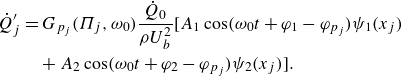 \begin{align} {{\dot Q}^{\prime}}_j & = G_{p_j}(\Pi _j,\omega _0) \frac {{\dot Q}_0}{\rho U_b^2} [A_1 \cos (\omega _0 t+\varphi _1-\varphi _{p_j})\psi _1(x_j)\nonumber\\& \quad +A_2 \cos (\omega _0 t+\varphi _2-\varphi _{p_j})\psi _2(x_j)] .\end{align}
It is here convenient to define
 $\tau _{p_j}=\varphi _{p_j}/\omega _0$
and write the previous expression as
$\tau _{p_j}=\varphi _{p_j}/\omega _0$
and write the previous expression as
 \begin{align} {{\dot Q}^{\prime}}_j & =G_{p_j}(\Pi _j,\omega _0) \frac {{\dot Q}_0}{\rho U_b^2} [A_1 \cos (\omega _0 (t-\tau _{p_j})+\varphi _1)\psi _1(x_j)\nonumber\\& \quad +A_2 \cos (\omega _0 (t-\tau _{p_j})+\varphi _2)\psi _2(x_j)] .\end{align}
One identifies in this expression the delayed pressure signal
 $p_j(t-\tau _{p_j})$
so that one may write
$p_j(t-\tau _{p_j})$
so that one may write
 \begin{equation} {{\dot Q}^{\prime}}_j=G_{p_j}(\Pi _j,\omega _0) \frac {{\dot Q}_0}{\rho U_b^2} p_j(t-\tau _{p_j}) .\end{equation}
Slow-flow variables
 $A_1, A_2, \varphi _1, \varphi _2$
and
$A_1, A_2, \varphi _1, \varphi _2$
and
 $\Pi _j$
being assumed constant over a period of oscillation, the time derivative of the HRR simply involves the rate of change of the pressure delayed by
$\Pi _j$
being assumed constant over a period of oscillation, the time derivative of the HRR simply involves the rate of change of the pressure delayed by
 $\tau _{p_j}$
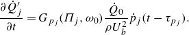 \begin{equation} \frac {\partial {{\dot Q}^{\prime}}_j}{\partial t} =G_{p_j}(\Pi _j,\omega _0) \frac {{\dot Q}_0}{\rho U_b^2} {\dot p}_j(t-\tau _{p_j}). \end{equation}
Comparing (5.8) and (5.17), one finds that
 \begin{equation} \mathcal {G}(\Pi _j, \omega _0) = G_{p_j}(\Pi _j,\omega _0)\frac {{\dot Q}_0}{\rho U_b^2} \end{equation}
and the dynamical system of (5.5) finally becomes
 \begin{align} {\ddot \eta }_1 & + \alpha {\dot \eta }_1 + \omega _0^2 \eta _1 =\frac {\gamma -1}{\Lambda }\sum _{j=1}^N G_{p_j} \frac {{\dot Q}_0}{\rho U_b^2} [{\dot \eta }_1(t-\tau _{p_j}) \psi _1(x_j)+{\dot \eta }_2 (t-\tau _{p_j}) \psi _2(x_j)] \psi _1(x_j) \nonumber\\ {\ddot \eta }_2 & + \alpha {\dot \eta }_2 + \omega _0^2 \eta _2 =\frac {\gamma -1}{\Lambda }\sum _{j=1}^N G_{p_j} \frac {{\dot Q}_0}{\rho U_b^2} [{\dot \eta }_1(t-\tau _{p_j}) \psi _1(x_j)+{\dot \eta }_2 (t-\tau _{p_j}) \psi _2(x_j)] \psi _2(x_j), \end{align}
where
 $G_{p_j}=G_{p_j}(\Pi _j,\omega _0)$
and the local oscillation amplitude
$G_{p_j}=G_{p_j}(\Pi _j,\omega _0)$
and the local oscillation amplitude
 $\Pi _j$
, expressed in terms of the slow-flow variables, reads
$\Pi _j$
, expressed in terms of the slow-flow variables, reads
 \begin{equation} \Pi _j=\frac {1}{\rho U_b^2 \sqrt {2}} \big[A_1^2\psi _1^2+A_2^2\psi _2^2+2A_1A_2\psi _1\psi _2\cos (\varphi _2-\varphi _1)\big]^{1/2}. \end{equation}
Using, in addition, the standard hypothesis of the method of averaging, the time derivative of the amplitude
 $\eta$
is
$\eta$
is
 \begin{align} {\dot \eta }_k&=-A_k(t) \omega _0 \sin (\omega _0 t+\varphi _k) \, \, \textrm {for}\,\, k=1,2,\end{align}
and one can express the slow-flow variables as a function of
 $\eta _k$
and
$\eta _k$
and
 ${\dot \eta }_k$
 \begin{equation} A_k= \left[{\eta _k^2+\left(\frac {{\dot \eta }_k}{\omega _0}\right)^2}\right]^{1/2}, \,\, \textrm {and} \,\, A_j A_k \cos (\varphi _j-\varphi _k)= \eta _j\eta _k+\frac {1}{\omega _0^2} {\dot \eta }_j {\dot \eta }_k .\end{equation}
The dynamics can hence be described by two coupled second-order oscillators. The coupling between the two eigenmodes appears on the right-hand side of these two equations, corresponding to the projection of the source term
 $S$
on each eigenmode. Equations (5.19) can be solved directly, as done, for instance, in Noiray et al. (Reference Noiray, Bothien and Schuermans2011). The integration is here carried out by making use of the FDF representation obtained in § 3. Typical examples of the direct integration of 5.19 are provided for staging patterns
$S$
on each eigenmode. Equations (5.19) can be solved directly, as done, for instance, in Noiray et al. (Reference Noiray, Bothien and Schuermans2011). The integration is here carried out by making use of the FDF representation obtained in § 3. Typical examples of the direct integration of 5.19 are provided for staging patterns
 $\mathcal {C}_0$
,
$\mathcal {C}_0$
,
 $\mathcal {C}_4$
,
$\mathcal {C}_4$
,
 $\mathcal {L}_4$
and
$\mathcal {L}_4$
and
 $\mathcal {A}_4$
and shown in figure 7 in the form of plots in the
$\mathcal {A}_4$
and shown in figure 7 in the form of plots in the
 $(\eta _1, \eta _2)$
plane. Circular trajectories in this plane found for
$(\eta _1, \eta _2)$
plane. Circular trajectories in this plane found for
 $\mathcal {C}_0$
or for
$\mathcal {C}_0$
or for
 $\mathcal {A}_4$
indicate that the oscillation at the limit cycle takes the form of a spinning mode. The elongated trajectories characterizing
$\mathcal {A}_4$
indicate that the oscillation at the limit cycle takes the form of a spinning mode. The elongated trajectories characterizing
 $\mathcal {C}_4$
or
$\mathcal {C}_4$
or
 $\mathcal {L}_4$
are typical of standing mode oscillations reflecting the symmetry breaking induced by the placement of four S injectors.
$\mathcal {L}_4$
are typical of standing mode oscillations reflecting the symmetry breaking induced by the placement of four S injectors.

Figure 7. Direct integration of the ordinary differential system with delay (5.19), for an initial condition
 $[\eta _1 =75, \dot {\eta }_1=50, \eta _2 =15, \dot {\eta }_2=10]$
, for configurations
$[\eta _1 =75, \dot {\eta }_1=50, \eta _2 =15, \dot {\eta }_2=10]$
, for configurations
 $\mathcal {C}_0$
,
$\mathcal {C}_0$
,
 $\mathcal {C}_4$
,
$\mathcal {C}_4$
,
 $\mathcal {L}_4$
and
$\mathcal {L}_4$
and
 $\mathcal {A}_4$
.
$\mathcal {A}_4$
.
5.4. Slow-flow equations
A further understanding of the system’s dynamics may be gained by deriving a set of equations for the slow-flow variables
 $A_1, A_2, \varphi _1$
and
$A_1, A_2, \varphi _1$
and
 $\varphi _2$
using the method of averaging. Solutions of (5.19) are now sought in the standard form
$\varphi _2$
using the method of averaging. Solutions of (5.19) are now sought in the standard form
 \begin{align}\eta _k & =A_k(t) \cos (\omega _0 t+\varphi _k) \nonumber\\ {\dot \eta }_k & =-A_k(t) \omega _0 \sin (\omega t+\varphi _k) \, \, \textrm {for}\,\, k=1,2. \end{align}
Using the same procedure as that described in § 4 and integrating over a period of oscillation
 $T=2\pi /\omega _0$
, this system yields the following equations for the slow-flow variables
$T=2\pi /\omega _0$
, this system yields the following equations for the slow-flow variables
 $A_1$
,
$A_1$
,
 $A_2$
,
$A_2$
,
 $\varphi _1$
and
$\varphi _1$
and
 $\varphi _2$
:
$\varphi _2$
:
 \begin{align} {\dot A}_1 & =-\frac {\alpha }{2} A_1 +\frac {\gamma -1}{2\Lambda } \frac {{\dot Q}_0}{\rho U_b^2}\sum _{j=1}^N G_{p_j} \big[A_1 \cos (\varphi _{p_j}) \psi _1(x_j)+A_2 \cos (\varphi _{p_j}\nonumber\\& \quad +\varphi _{12})\psi _2(x_j)\big]\psi _1(x_j)\nonumber\\ {\dot A}_2& =-\frac {\alpha }{2} A_2 +\frac {\gamma -1}{2\Lambda } \frac {{\dot Q}_0}{\rho U_b^2}\sum _{j=1}^N G_{p_j} \big[A_2 \cos (\varphi _{p_j}) \psi _2(x_j)+A_1 \cos (\varphi _{p_j}\nonumber\\& \quad +\varphi _{21})\psi _1(x_j)\big]\psi _2(x_j)\nonumber\\ A_1 {\dot \varphi }_1& = \frac {\gamma -1}{\Lambda }\frac {{\dot Q}_0}{\rho U_b^2} \sum _{j=1}^N G_{p_j} \big[-A_1 \sin (\varphi _{p_j}) \psi _1^2(x_j) +A_2 \sin (\varphi _{21}-\varphi _{p_j})\psi _1(x_j)\psi _2(x_j)\big]\nonumber\\ A_2 {\dot \varphi }_2& = \frac {\gamma -1}{\Lambda } \frac {{\dot Q}_0}{\rho U_b^2}\sum _{j=1}^N G_{p_j} \big[-A_2 \sin (\varphi _{p_j}) \psi _2^2(x_j) +A_1 \sin (\varphi _{12}-\varphi _{p_j})\psi _1(x_j)\psi _2(x_j)\big].\end{align}
In these equations
 $\varphi _{12}=\varphi _1-\varphi _2$
,
$\varphi _{12}=\varphi _1-\varphi _2$
,
 $\varphi _{21}=\varphi _2-\varphi _1$
and the gains and phases,
$\varphi _{21}=\varphi _2-\varphi _1$
and the gains and phases,
 $G_{p_j} =G_j (\Pi _j,\omega _0)$
and
$G_{p_j} =G_j (\Pi _j,\omega _0)$
and
 $\varphi _{p_j}=\varphi _{p_j}(\Pi _j,\omega _0)$
, correspond to the flames established by the different injectors, with
$\varphi _{p_j}=\varphi _{p_j}(\Pi _j,\omega _0)$
, correspond to the flames established by the different injectors, with
 $\Pi _j=(p_{rms})_j/(\rho U_b^2)$
, the dimensionless pressure amplitude at flame
$\Pi _j=(p_{rms})_j/(\rho U_b^2)$
, the dimensionless pressure amplitude at flame
 $j$
, which is expressed in terms of the slow-flow variables in (5.20).
$j$
, which is expressed in terms of the slow-flow variables in (5.20).
It is also interesting to deduce an evolution equation for the difference
 $\varphi _1-\varphi _2$
. This can be done by multiplying the third equation in the set (5.24) by
$\varphi _1-\varphi _2$
. This can be done by multiplying the third equation in the set (5.24) by
 $A_2$
and subtracting the fourth equation in this set after multiplication by
$A_2$
and subtracting the fourth equation in this set after multiplication by
 $A_1$
. This yields
$A_1$
. This yields
 \begin{align} A_1A_2 (\dot {\varphi }_1- \dot {\varphi }_2) & = \frac {(\gamma -1)}{\Lambda } \frac {{\dot Q}_0}{\rho U_b^2} \sum _{j=1}^N G_{p_j} \Big \{A_1A_2 \sin (\varphi _{p_j})[\psi _2^2(x_j)- \psi _1^2(x_j)]\nonumber\\& \quad -A_1^2 \sin (\varphi _1-\varphi _2-\varphi _{p_j})\psi _1(x_j)\psi _2(x_j)\nonumber\\& \quad + A_2^2 \sin (\varphi _2-\varphi _1-\varphi _{p_j})\psi _1(x_j)\psi _2(x_j) \Big \} .\end{align}
A comprehensive discussion on the theoretical conditions for the stability of fixed standing and spinning solutions of the system formed by (5.24) can be found in Ghirardo et al. (Reference Ghirardo, Juniper and Moeck2016). Additional terms due to turbulence-induced acoustic forcing were not considered in the present work, because, as will be seen in § 5.5, the dynamical equations, in the form proposed in (5.24), enable us to reasonably retrieve the features observed experimentally, which are mainly dominated by symmetry-breaking effects induced by injectors’ staging. There is, however, one exception, in the special case were all injectors are of the same kind: we will see that the dynamical equations predict a limit cycle in the form of a purely spinning wave, while experiments indicate that the system continuously switches between spinning modes and mixed modes of various types. In that case, the stochastic term representing turbulent disturbances might probably be necessary to obtain a suitable match with observations (on that point see Ghirardo et al. Reference Ghirardo, Boudy and Bothien2018).
5.5. Application to staging patterns in MICCA-spray
The system of ordinary differential equations (ODEs) obtained in § 5.4 is now solved for different configurations mixing U- and S-injectors in MICCA, shown in figure 6. For all the staging patterns tested, the instability frequencies lie between 775 and 820 Hz and the oscillation amplitudes between 100 and 1400 Pa. Further details on the experimental results may be found in Latour et al. (Reference Latour, Durox, Renaud and Candel2024a ).
Expressions for
 $G_{p_j}(\Pi _j,\omega _0)$
and
$G_{p_j}(\Pi _j,\omega _0)$
and
 $\varphi _{p_j}(\Pi _j,\omega _0)$
are those deduced from experimental data for the two injection units U and S, collected for a range of frequencies close to the eigenfrequency of the 1A1L mode of the MICCA combustor and reported in § 3. One can reasonably model the gain of the pressure-based FDF as
$\varphi _{p_j}(\Pi _j,\omega _0)$
are those deduced from experimental data for the two injection units U and S, collected for a range of frequencies close to the eigenfrequency of the 1A1L mode of the MICCA combustor and reported in § 3. One can reasonably model the gain of the pressure-based FDF as
 $G_{p_j}=\beta -\kappa \Pi _j$
, as discussed in § 3. The coefficients
$G_{p_j}=\beta -\kappa \Pi _j$
, as discussed in § 3. The coefficients
 $\beta$
and
$\beta$
and
 $\kappa$
for injectors U and S are deduced from a linear regression of the
$\kappa$
for injectors U and S are deduced from a linear regression of the
 $G_p=G_p(\Pi )$
data points. The phases,
$G_p=G_p(\Pi )$
data points. The phases,
 $\varphi _S$
and
$\varphi _S$
and
 $\varphi _U$
, are assumed to be constant and equal to the mean value, as shown by the experimental results reported in figure 4, where the phases for the two injectors take nearly constant values throughout the range of pressure amplitudes tested. Noting that the damping rate
$\varphi _U$
, are assumed to be constant and equal to the mean value, as shown by the experimental results reported in figure 4, where the phases for the two injectors take nearly constant values throughout the range of pressure amplitudes tested. Noting that the damping rate
 $\alpha$
describes the rate of change in acoustic energy (i.e. of pressure squared), the damping rate used for the numerical integration is assigned a value that is twice that obtained by Latour et al. (Reference Latour, Durox, Renaud and Candel2024b
), where the damping rate for the pressure is extracted from direct measurements of the Rayleigh source term while operating the MICCA combustor at limit cycle. It is also assumed that the damping rate value does not change with the staging pattern and may be represented by a constant value.
$\alpha$
describes the rate of change in acoustic energy (i.e. of pressure squared), the damping rate used for the numerical integration is assigned a value that is twice that obtained by Latour et al. (Reference Latour, Durox, Renaud and Candel2024b
), where the damping rate for the pressure is extracted from direct measurements of the Rayleigh source term while operating the MICCA combustor at limit cycle. It is also assumed that the damping rate value does not change with the staging pattern and may be represented by a constant value.
As pointed out by a reviewer, there are cases where the damping depends nonlinearly on the level of oscillation. For example, damping by Helmholtz resonators is a function of the level of oscillation, as shown by Zinn & Lores (Reference Zinn and Lores1972) or Ćosić, Reichel & Paschereit (Reference Ćosić, Reichel and Paschereit2012). The nonlinearity is, in this case, linked to the vortex shedding from the resonator outlet. The use of perforated liners or quarter wave cavities also introduces nonlinearities as indicated for example by Schuller et al. (Reference Schuller, Tran, Noiray, Durox, Ducruix and Candel2009). However, MICCA is not equipped with such devices and the damping nonlinearity is less probable. In addition, the damping rates of acoustic energy estimated in MICCA from energy balance considerations at various limit-cycle amplitudes for a range of limit-cycle oscillation levels (670–1400 Pa) by Latour et al. (Reference Latour, Durox, Renaud and Candel2024b ) show no amplitude dependence, as can be seen in figure 8. There are only minor variations in the damping rate for the different oscillation levels and one may safely conclude that nonlinearities need not be taken into consideration.
Using the parameters gathered in table 2, the differential equations are integrated with the MATLAB ode45 solver. Typical results shown in figure 9 pertain to the four staging patterns
 $\mathcal {C}_0, \mathcal {C}_4, \mathcal {L}_4$
and
$\mathcal {C}_0, \mathcal {C}_4, \mathcal {L}_4$
and
 $\mathcal {A}_4$
.
$\mathcal {A}_4$
.
Table 2. Pressure-based FDFs and damping rate used in the numerical simulations.


Figure 8. Damping rate values as a function of the oscillation level
 ${A}$
obtained from source term and acoustic energy estimates in MICCA during self-sustained limit-cycle oscillations for different staging configurations Latour et al. (Reference Latour, Durox, Renaud and Candel2024b
). The annular combustor is operated at a thermal power
${A}$
obtained from source term and acoustic energy estimates in MICCA during self-sustained limit-cycle oscillations for different staging configurations Latour et al. (Reference Latour, Durox, Renaud and Candel2024b
). The annular combustor is operated at a thermal power
 $\mathcal {P}=118\,\textrm{kW}$
and an equivalence ratio
$\mathcal {P}=118\,\textrm{kW}$
and an equivalence ratio
 $\phi =0.9$
.
$\phi =0.9$
.
In the
 $\mathcal {C}_0$
case, the amplitudes
$\mathcal {C}_0$
case, the amplitudes
 $A_1$
and
$A_1$
and
 $A_2$
grow to the limit cycle in approximately
$A_2$
grow to the limit cycle in approximately
 $25$
ms and take the same value, while the phase difference
$25$
ms and take the same value, while the phase difference
 $\varphi _1-\varphi _2$
tends to
$\varphi _1-\varphi _2$
tends to
 $\pi /2$
, indicating that the mode is a spinning wave. For configurations
$\pi /2$
, indicating that the mode is a spinning wave. For configurations
 $\mathcal {C}_4$
and
$\mathcal {C}_4$
and
 $\mathcal {L}_4$
, the amplitudes reach constant levels while the phase difference
$\mathcal {L}_4$
, the amplitudes reach constant levels while the phase difference
 $\varphi _1-\varphi _2$
tends to zero. The oscillation now corresponds to a standing mode. The anti-nodal line angle
$\varphi _1-\varphi _2$
tends to zero. The oscillation now corresponds to a standing mode. The anti-nodal line angle
 $\theta _0$
may be deduced from the values of
$\theta _0$
may be deduced from the values of
 $A_1$
and
$A_1$
and
 $A_2$
at limit cycle, using the expression
$A_2$
at limit cycle, using the expression
 $\theta _0 = \arccos [A_1/ (A_1^2+ A_2^2)^{1/2}]$
. The nodal line found analytically is aligned with the diameter joining the two groups of S-injectors in diametrically opposed locations for
$\theta _0 = \arccos [A_1/ (A_1^2+ A_2^2)^{1/2}]$
. The nodal line found analytically is aligned with the diameter joining the two groups of S-injectors in diametrically opposed locations for
 $\mathcal {L}_4$
and passes at equal distance of the four S injectors in configuration
$\mathcal {L}_4$
and passes at equal distance of the four S injectors in configuration
 $\mathcal {C}_4$
. These analytical results correspond to those found experimentally (Latour et al. Reference Latour, Durox, Renaud and Candel2024a
). Finally, in case
$\mathcal {C}_4$
. These analytical results correspond to those found experimentally (Latour et al. Reference Latour, Durox, Renaud and Candel2024a
). Finally, in case
 $\mathcal {A}_4$
, the growth in amplitude is less rapid than in the
$\mathcal {A}_4$
, the growth in amplitude is less rapid than in the
 $\mathcal {C}_0$
case and the levels at limit cycle are also lower. Similarly to configuration
$\mathcal {C}_0$
case and the levels at limit cycle are also lower. Similarly to configuration
 $\mathcal {C}_0$
,
$\mathcal {C}_0$
,
 $A_1$
is equal to
$A_1$
is equal to
 $A_2$
while
$A_2$
while
 $\varphi _1-\varphi _2$
tends to
$\varphi _1-\varphi _2$
tends to
 $\pi /2$
, which correspond to a spinning wave.
$\pi /2$
, which correspond to a spinning wave.

Figure 9. Slow-flow variables
 $A_1, A_2$
and
$A_1, A_2$
and
 $\varphi _1-\varphi _2$
time evolutions for configurations
$\varphi _1-\varphi _2$
time evolutions for configurations
 $\mathcal {C}_0$
,
$\mathcal {C}_0$
,
 $\mathcal { C}_4$
,
$\mathcal { C}_4$
,
 $\mathcal {L}_4$
and
$\mathcal {L}_4$
and
 $\mathcal {A}_4$
, obtained from the resolution of the ordinary differential equations for the initial conditions
$\mathcal {A}_4$
, obtained from the resolution of the ordinary differential equations for the initial conditions
 $A_1=50\,\textrm{Pa}$
,
$A_1=50\,\textrm{Pa}$
,
 $A_2=75\,\textrm{Pa}$
,
$A_2=75\,\textrm{Pa}$
,
 $\varphi _1-\varphi _2=0.1\,\textrm{rad}$
.
$\varphi _1-\varphi _2=0.1\,\textrm{rad}$
.
It is next interesting to examine the predicted limit-cycle amplitudes and compare them with the values measured experimentally. This comparison may be carried out by making use of the link between the amplitude
 $A=(A_+^2+A_-^2)^{1/2}$
that is used in the experimental determination of the limit-cycle amplitudes (see § 2, (2.3) and Latour et al. Reference Latour, Durox, Renaud and Candel2024a
) and the amplitudes
$A=(A_+^2+A_-^2)^{1/2}$
that is used in the experimental determination of the limit-cycle amplitudes (see § 2, (2.3) and Latour et al. Reference Latour, Durox, Renaud and Candel2024a
) and the amplitudes
 $A_1$
and
$A_1$
and
 $A_2$
of the eigenmodes
$A_2$
of the eigenmodes
 $\psi _1$
and
$\psi _1$
and
 $\psi _2$
, intervening in (5.24). It is shown in Appendix D that
$\psi _2$
, intervening in (5.24). It is shown in Appendix D that
 \begin{equation} A=\big(A_+^2+A_-^2\big)^{1/2}=\frac {1}{{2^{1/2}}} \big(A_1^2+A_2^2\big)^{1/2} .\end{equation}

Figure 10. (a) Limit-cycle oscillation amplitudes obtained by integrating the system of ODEs for the slow-flow variables for the three types of staging configurations investigated (type
 $\mathcal{C}$
,
$\mathcal{C}$
,
 $\mathcal{L}$
and
$\mathcal{L}$
and
 $\mathcal{A}$
). (b,c,d) Comparison of the limit-cycle oscillation amplitudes measured experimentally (Latour et al. Reference Latour, Durox, Renaud and Candel2024a
) and obtained by solving the system of ODEs for the slow-flow variables for type
$\mathcal{A}$
). (b,c,d) Comparison of the limit-cycle oscillation amplitudes measured experimentally (Latour et al. Reference Latour, Durox, Renaud and Candel2024a
) and obtained by solving the system of ODEs for the slow-flow variables for type
 $\mathcal{C}$
(b),
$\mathcal{C}$
(b),
 $\mathcal{L}$
(c) and
$\mathcal{L}$
(c) and
 $\mathcal{A}$
(d) configurations. Here
$\mathcal{A}$
(d) configurations. Here
 $N_S$
corresponds to the number of S-injectors.
$N_S$
corresponds to the number of S-injectors.
The predicted limit-cycle oscillation amplitudes
 $A$
, deduced by solving the slow-flow equations for
$A$
, deduced by solving the slow-flow equations for
 $A_1$
and
$A_1$
and
 $A_2$
and making use of 5.26, are displayed in figure 10. The amplitude
$A_2$
and making use of 5.26, are displayed in figure 10. The amplitude
 $A$
decreases when the number of S-injectors is increased and the trends corresponding to type
$A$
decreases when the number of S-injectors is increased and the trends corresponding to type
 $\mathcal{C}$
arrangements clearly differ from those pertaining to
$\mathcal{C}$
arrangements clearly differ from those pertaining to
 $\mathcal{L}$
configurations. A comparison with the experimental data from Latour et al. (Reference Latour, Durox, Renaud and Candel2024a
) is carried out in figure 10(b,c,d) where the
$\mathcal{L}$
configurations. A comparison with the experimental data from Latour et al. (Reference Latour, Durox, Renaud and Candel2024a
) is carried out in figure 10(b,c,d) where the
 $\mathcal{C}$
,
$\mathcal{C}$
,
 $\mathcal{L}$
and
$\mathcal{L}$
and
 $\mathcal{A}$
configurations appear in three separate graphs. The match obtained between experimental data and model prediction is, despite some differences, quite satisfactory. The limit-cycle amplitudes cover the same range with a maximum value of slightly less than 1500 Pa. Configurations
$\mathcal{A}$
configurations appear in three separate graphs. The match obtained between experimental data and model prediction is, despite some differences, quite satisfactory. The limit-cycle amplitudes cover the same range with a maximum value of slightly less than 1500 Pa. Configurations
 $\mathcal {C}_8$
and
$\mathcal {C}_8$
and
 $\mathcal {A}_8$
, which are experimentally stable, are suitably predicted by the model as having a low level of oscillation. The decrease in amplitude observed when the staging patterns is evolving from
$\mathcal {A}_8$
, which are experimentally stable, are suitably predicted by the model as having a low level of oscillation. The decrease in amplitude observed when the staging patterns is evolving from
 $\mathcal {C}_0$
to
$\mathcal {C}_0$
to
 $\mathcal {C}_8$
is well retrieved but the calculated amplitudes are slightly higher than those measured experimentally.
$\mathcal {C}_8$
is well retrieved but the calculated amplitudes are slightly higher than those measured experimentally.
The trends observed experimentally for the
 $\mathcal{L}$
-type staging patterns, where the limit-cycle amplitude levels decrease more slowly than for type
$\mathcal{L}$
-type staging patterns, where the limit-cycle amplitude levels decrease more slowly than for type
 $\mathcal{C}$
configurations as the number of S-injectors is augmented, are also found with the model, although larger discrepancies are observed between experimental data and simulation for these configurations. The greatest differences in limit-cycle amplitudes are found for
$\mathcal{C}$
configurations as the number of S-injectors is augmented, are also found with the model, although larger discrepancies are observed between experimental data and simulation for these configurations. The greatest differences in limit-cycle amplitudes are found for
 $\mathcal {C}_4$
,
$\mathcal {C}_4$
,
 $\mathcal {L}_4$
and
$\mathcal {L}_4$
and
 $\mathcal {A}_4$
. This may be due to a different damping rate value for these staging arrangements (Latour et al. Reference Latour, Durox, Renaud and Candel2024b
) that is not accounted for in the modelling. It is also possible that some adjustment of the gain
$\mathcal {A}_4$
. This may be due to a different damping rate value for these staging arrangements (Latour et al. Reference Latour, Durox, Renaud and Candel2024b
) that is not accounted for in the modelling. It is also possible that some adjustment of the gain
 $G_p^S$
corresponding to the S-injectors might have improved the prediction, but no attempt was made to go in that direction. As indicated in § 3, the gain and phase values for S-injectors are less well determined because these units are located in regions where the oscillation level is low and this influences the measurement precision. Another possibility could be that the gain
$G_p^S$
corresponding to the S-injectors might have improved the prediction, but no attempt was made to go in that direction. As indicated in § 3, the gain and phase values for S-injectors are less well determined because these units are located in regions where the oscillation level is low and this influences the measurement precision. Another possibility could be that the gain
 $G_p$
is influenced to some extent by the nature of the mode as inferred by Nygård, Ghirardo & Worth (2021) and Ghirardo et al. (Reference Ghirardo, Nygård, Cuquel and Worth2021), and that this might have to be accounted for in the pressure-based FDF formulation. However, although some discrepancies exist between experimental data and model predictions, this is perhaps the first time where calculations are shown to be capable of predicting limit-cycle levels of oscillation for a large set of experiments.
$G_p$
is influenced to some extent by the nature of the mode as inferred by Nygård, Ghirardo & Worth (2021) and Ghirardo et al. (Reference Ghirardo, Nygård, Cuquel and Worth2021), and that this might have to be accounted for in the pressure-based FDF formulation. However, although some discrepancies exist between experimental data and model predictions, this is perhaps the first time where calculations are shown to be capable of predicting limit-cycle levels of oscillation for a large set of experiments.
It is next interesting to examine the distribution of the r.m.s. of the pressure field as a function of the azimuthal position deduced from the numerical integration of the slow-flow equations. This distribution is shown in figure 11 for all the staging configurations. The first row in this figure corresponds to
 $\mathcal{C}$
configurations. For
$\mathcal{C}$
configurations. For
 $\mathcal {C}_0$
, where all injectors are of the U-type, the r.m.s. pressure distribution is uniform, as expected for a spinning mode. As S-injectors are being added to replace U-injectors, the r.m.s. pressure distribution features two maximum and two minimum values. The minimum is reached at the location of the S-injector (case
$\mathcal {C}_0$
, where all injectors are of the U-type, the r.m.s. pressure distribution is uniform, as expected for a spinning mode. As S-injectors are being added to replace U-injectors, the r.m.s. pressure distribution features two maximum and two minimum values. The minimum is reached at the location of the S-injector (case
 $\mathcal {C}_1$
) or on the diameter passing through the centre of the
$\mathcal {C}_1$
) or on the diameter passing through the centre of the
 $\mathcal{C}$
configuration as exemplified by
$\mathcal{C}$
configuration as exemplified by
 $\mathcal { C}_2$
,
$\mathcal { C}_2$
,
 $\mathcal {C}_4$
and
$\mathcal {C}_4$
and
 $\mathcal {C}_6$
. In the last two cases, the minimum r.m.s. pressure is close to zero, corresponding to a standing mode. In case
$\mathcal {C}_6$
. In the last two cases, the minimum r.m.s. pressure is close to zero, corresponding to a standing mode. In case
 $\mathcal {C}_8$
, the calculated level of oscillation is very low, indicating that the system is stable. The second row shows the r.m.s. pressure distributions for
$\mathcal {C}_8$
, the calculated level of oscillation is very low, indicating that the system is stable. The second row shows the r.m.s. pressure distributions for
 $\mathcal{L}$
and
$\mathcal{L}$
and
 $\mathcal{A}$
cases. The minimum values are observed on the diameter that passes through the S-injectors (case
$\mathcal{A}$
cases. The minimum values are observed on the diameter that passes through the S-injectors (case
 $\mathcal {L}_{2}$
) or on the median diameter of the S-injector configurations (
$\mathcal {L}_{2}$
) or on the median diameter of the S-injector configurations (
 $\mathcal {L}_{4}$
,
$\mathcal {L}_{4}$
,
 $\mathcal {L}_{6}$
,
$\mathcal {L}_{6}$
,
 $\mathcal {L}_{8}$
). In the last three cases, the minimum value is close to zero, a clear signature of a standing mode. The cases
$\mathcal {L}_{8}$
). In the last three cases, the minimum value is close to zero, a clear signature of a standing mode. The cases
 $\mathcal {A}_4$
and
$\mathcal {A}_4$
and
 $\mathcal {A}_8$
feature a uniform distribution of r.m.s. pressure as the symmetry is not broken by the presence of the 4 or 8 S-injectors. In case
$\mathcal {A}_8$
feature a uniform distribution of r.m.s. pressure as the symmetry is not broken by the presence of the 4 or 8 S-injectors. In case
 $\mathcal {A}_4$
, the amplitude is reduced but not to the point observed experimentally (this configuration is marginally unstable). In
$\mathcal {A}_4$
, the amplitude is reduced but not to the point observed experimentally (this configuration is marginally unstable). In
 $\mathcal {A}_8$
, the level is quite low and the system is stable.
$\mathcal {A}_8$
, the level is quite low and the system is stable.

Figure 11. Root mean square of the pressure distribution as a function of the azimuthal position
 $\theta$
obtained from the numerical integration of the ODEs for the slow-flow variables. The red vertical lines correspond to S-injectors positions.
$\theta$
obtained from the numerical integration of the ODEs for the slow-flow variables. The red vertical lines correspond to S-injectors positions.
The previous calculations already show typical consequences of the breaking of symmetry in various configurations. These features generally retrieve those found in experiments. For example, it is known that the presence of a single S-injector in
 $\mathcal {C}_1$
is insufficient to break the symmetry and the pressure distribution only shows weak undulations. In cases
$\mathcal {C}_1$
is insufficient to break the symmetry and the pressure distribution only shows weak undulations. In cases
 $\mathcal {C}_4$
and
$\mathcal {C}_4$
and
 $\mathcal {C}_6$
and in arrangements
$\mathcal {C}_6$
and in arrangements
 $\mathcal {L}_{4}$
,
$\mathcal {L}_{4}$
,
 $\mathcal {L}_{6}$
and
$\mathcal {L}_{6}$
and
 $\mathcal {L}_{8}$
, symmetry is broken, giving rise to a standing mode and this agrees well with what is found experimentally (see Latour et al. Reference Latour, Durox, Renaud and Candel2024b
). It is, however, interesting to pursue the examination of the nature of the unstable mode by computing the spin ratio, initially defined by Bourgouin et al. (Reference Bourgouin, Durox, Moeck, Schuller and Candel2013) in terms of azimuthal wave amplitudes
$\mathcal {L}_{8}$
, symmetry is broken, giving rise to a standing mode and this agrees well with what is found experimentally (see Latour et al. Reference Latour, Durox, Renaud and Candel2024b
). It is, however, interesting to pursue the examination of the nature of the unstable mode by computing the spin ratio, initially defined by Bourgouin et al. (Reference Bourgouin, Durox, Moeck, Schuller and Candel2013) in terms of azimuthal wave amplitudes
 $A_+, A_-$
as
$A_+, A_-$
as
 \begin{equation} s_r= \frac {A_+ - A_-}{A_+ + A_-} .\end{equation}
It is worth remembering that the nature angle
 $\chi$
, that is used in many recent studies of azimuthal instabilities (see for instance Ghirardo & Bothien Reference Ghirardo and Bothien2018; Faure-Beaulieu & Noiray Reference Faure-Beaulieu and Noiray2020; Indlekofer et al. Reference Indlekofer, Faure-Beaulieu, Dawson and Noiray2022), is linked to the the spin ratio by
$\chi$
, that is used in many recent studies of azimuthal instabilities (see for instance Ghirardo & Bothien Reference Ghirardo and Bothien2018; Faure-Beaulieu & Noiray Reference Faure-Beaulieu and Noiray2020; Indlekofer et al. Reference Indlekofer, Faure-Beaulieu, Dawson and Noiray2022), is linked to the the spin ratio by
 $\chi = \tan ^{-1}s_r$
.
$\chi = \tan ^{-1}s_r$
.
Now,
 $s_r$
may be expressed in terms of the amplitudes
$s_r$
may be expressed in terms of the amplitudes
 $A_1$
and
$A_1$
and
 $A_2$
of the eigenmodes
$A_2$
of the eigenmodes
 $\psi _1$
and
$\psi _1$
and
 $\psi _2$
using relations derived in Appendix D. One gets
$\psi _2$
using relations derived in Appendix D. One gets
 \begin{equation} s_r= \frac {A_1A_2 \sin (\varphi _1-\varphi _2)\cos 2\theta _0}{A_1^2\cos ^2 \theta _0-A_2^2\sin ^2 \theta _0} ,\end{equation}
where
 $\theta _0$
is the anti-nodal line position, which is also expressed in terms of
$\theta _0$
is the anti-nodal line position, which is also expressed in terms of
 $A_1$
and
$A_1$
and
 $A_2$
in Appendix D.
$A_2$
in Appendix D.
Statistics for the experimental nodal line position, spin ratio time series and joint probability density functions for
 $A_+$
and
$A_+$
and
 $A_-$
can be found in Latour et al. (Reference Latour, Durox, Renaud and Candel2024a
). The nature of the mode at limit cycle is here represented by placing the limit-cycle characteristics of the unstable configurations, obtained from the resolution of the ODEs, in the (
$A_-$
can be found in Latour et al. (Reference Latour, Durox, Renaud and Candel2024a
). The nature of the mode at limit cycle is here represented by placing the limit-cycle characteristics of the unstable configurations, obtained from the resolution of the ODEs, in the (
 $|s_r|$
,
$|s_r|$
,
 $A$
) plane, as shown in figure 12. In cases
$A$
) plane, as shown in figure 12. In cases
 $\mathcal {C}_0$
and
$\mathcal {C}_0$
and
 $\mathcal {A}_4$
, one finds
$\mathcal {A}_4$
, one finds
 $|s_r|=1$
, corresponding to a purely spinning mode. While calculations for symmetric unstable configurations lead to a spinning mode, experiments indicate that the spin ratio continuously changes between -1 and +1. This difference in behaviour between calculations and experiments confirms findings by Noiray et al. (Reference Noiray, Bothien and Schuermans2011) and Faure-Beaulieu & Noiray (Reference Faure-Beaulieu and Noiray2020) and is due, according to these authors, to the absence of a stochastic forcing. Such a forcing, which idealizes the effect of turbulence, is needed to obtain a variable spin ratio taking values over the interval
$|s_r|=1$
, corresponding to a purely spinning mode. While calculations for symmetric unstable configurations lead to a spinning mode, experiments indicate that the spin ratio continuously changes between -1 and +1. This difference in behaviour between calculations and experiments confirms findings by Noiray et al. (Reference Noiray, Bothien and Schuermans2011) and Faure-Beaulieu & Noiray (Reference Faure-Beaulieu and Noiray2020) and is due, according to these authors, to the absence of a stochastic forcing. Such a forcing, which idealizes the effect of turbulence, is needed to obtain a variable spin ratio taking values over the interval
 $[-1,+1]$
.
$[-1,+1]$
.
It is also concluded from figure 12 that:
-
(i) Weak asymmetry in the staging pattern leads to a mixed mode (
$\mathcal {C}_1$
,
$\mathcal {C}_2$
and
$\mathcal {L}_2$
). -
(ii) Strong asymmetry in the staging pattern gives rise to a standing mode (
$\mathcal {C}_4$
,
$\mathcal {C}_6$
,
$\mathcal { L}_4$
,
$\mathcal {L}_6$
and
$\mathcal {L}_8$
), with the nodal line aligned with the S-injectors median diameter. When standing modes prevail, the nodal line position predicted analytically corresponds to that observed experimentally.


Figure 12. Unstable configurations in the (
 $A$
,
$A$
,
 $s_r$
) plane.
$s_r$
) plane.
5.6. Sensitivity analysis
It is natural at this stage to examine the sensitivity of the limit-cycle amplitudes to the choice of the FDF gain formulation and fitting coefficients. This is done here for the linear and quadratic fits shown in figure 13 for injectors U and S. The linear fit used in § 5.4 is first compared with a quadratic FDF gain formulation of the form
 $G_p=\beta -\kappa \Pi ^2$
. The predicted limit-cycle amplitudes are shown for the linear and quadratic expressions in figure 14(a) for type
$G_p=\beta -\kappa \Pi ^2$
. The predicted limit-cycle amplitudes are shown for the linear and quadratic expressions in figure 14(a) for type
 $\mathcal{C}$
configurations. One can see that both formulations lead to similar trends and oscillation amplitude values.
$\mathcal{C}$
configurations. One can see that both formulations lead to similar trends and oscillation amplitude values.
The sensitivity of the calculated amplitudes to the regression coefficients is then tested by changing by
 $\pm 5\, \%$
the fitted
$\pm 5\, \%$
the fitted
 $\beta$
and
$\beta$
and
 $\kappa$
values for injector U. Results of this analysis are plotted in figure 14(b,c) for the linear fit, for type
$\kappa$
values for injector U. Results of this analysis are plotted in figure 14(b,c) for the linear fit, for type
 $\mathcal{C}$
configurations. One can see that the calculated results are most sensitive to
$\mathcal{C}$
configurations. One can see that the calculated results are most sensitive to
 $\beta$
as a
$\beta$
as a
 $\pm 5\, \%$
change in the value of this parameter induces a
$\pm 5\, \%$
change in the value of this parameter induces a
 $\pm 200\,\textrm{Pa}$
variation in the limit-cycle amplitude. A
$\pm 200\,\textrm{Pa}$
variation in the limit-cycle amplitude. A
 $\pm 5\, \%$
change in
$\pm 5\, \%$
change in
 $\kappa$
has a lesser impact on the predicted limit-cycle oscillation amplitudes. A similar sensitivity analysis for the quadratic fit, not reproduced here, leads to the same conclusions.
$\kappa$
has a lesser impact on the predicted limit-cycle oscillation amplitudes. A similar sensitivity analysis for the quadratic fit, not reproduced here, leads to the same conclusions.

Figure 13. Linear (a,b) and quadratic (c,d) fits for the pressure-based FDF gain experimental data for injector U (a,c) and injector S (b,d).

Figure 14. Comparison between a linear and a quadratic expression for the FDF gain on the limit-cycle oscillation amplitude (a). Effects of a
 $\pm 5\%$
change in the
$\pm 5\%$
change in the
 $\beta$
(b) and
$\beta$
(b) and
 $\kappa$
(c) coefficients values on the analytical limit-cycle oscillation amplitudes for type
$\kappa$
(c) coefficients values on the analytical limit-cycle oscillation amplitudes for type
 $\mathcal{C}$
configurations. Here
$\mathcal{C}$
configurations. Here
 $N_S$
corresponds to the number of S-injectors.
$N_S$
corresponds to the number of S-injectors.
6. Determination of growth rate and comparison with that deduced from an acoustic energy balance
The dynamical equations for the slow-flow variables describe the evolution of the system as a function of time. It is interesting to ask whether these equations can be used to derive an expression for the instantaneous growth rate and, in a second stage, compare this expression with that obtained by Latour et al. (Reference Latour, Durox, Renaud and Candel2024a
) by making use of energy balance principles. As we will see, this comparison is not straightforward because one has to link the slow variables
 $A_1$
and
$A_1$
and
 $A_2$
, corresponding to the amplitudes of the two perpendicular standing modes
$A_2$
, corresponding to the amplitudes of the two perpendicular standing modes
 $\psi _1$
and
$\psi _1$
and
 $\psi _2$
, to the amplitudes
$\psi _2$
, to the amplitudes
 $A_{+}$
and
$A_{+}$
and
 $ A_{-}$
, associated with the azimuthal waves propagating in the CCW and CW directions. This requires some algebra but allows a term by term comparison between expressions obtained in two notably different ways.
$ A_{-}$
, associated with the azimuthal waves propagating in the CCW and CW directions. This requires some algebra but allows a term by term comparison between expressions obtained in two notably different ways.
We specifically consider the evolution of
 $A_1^2+A_2^2$
and wish to deduce the effective growth rate, defined as
$A_1^2+A_2^2$
and wish to deduce the effective growth rate, defined as
 $\omega^{\prime}_i=\omega _i -\alpha /2$
, from the logarithmic derivative of this quantity
$\omega^{\prime}_i=\omega _i -\alpha /2$
, from the logarithmic derivative of this quantity
 \begin{equation} \omega^{\prime}_i = \frac {1}{2} \frac {1}{\big(A_1^2+A_2^2\big)}\frac{\textrm{d}}{\textrm{d}\it t}\big(A_1^2+A_2^2\big). \end{equation}
Multiplying the first two equations in the system 5.24 by
 $A_1$
and
$A_1$
and
 $A_2$
, respectively, one obtains
$A_2$
, respectively, one obtains
 \begin{align} \frac {1}{2} \frac {\textrm{d}A_1^2}{\textrm{d}\it t} & = -\frac {\alpha }{2}A_1^2 +\frac { \gamma -1}{2 \Lambda } \sum _{j=1}^N \frac {{\dot Q}_0}{\rho U_b^2}G_{p_j}\big [A_1^2 \cos \varphi _{p_j} \cos ^2\theta _j\nonumber\\& \quad + A_2A_1 \cos (\varphi _{p_j}+\varphi _{12}) \sin \theta _j\cos \theta _j\big ]\nonumber\\ \frac {1}{2} \frac {\textrm{d}A_2^2}{\textrm{d}\it t} & = -\frac {\alpha }{2}A_2^2 +\frac { \gamma -1}{2 \Lambda } \sum _{j=1}^N \frac {{\dot Q}_0}{\rho U_b^2}G_{p_j}\big [A_2^2 \cos \varphi _{p_j} \sin ^2\theta _j\nonumber\\& \quad + A_1A_2 \cos (\varphi _{p_j}+\varphi _{21}) \sin \theta _j\cos \theta _j\big ], \end{align}
where
 $\varphi _{12}=\varphi _1-\varphi _2= -\varphi _{21}$
. These two equations may be summed and the result, when divided by
$\varphi _{12}=\varphi _1-\varphi _2= -\varphi _{21}$
. These two equations may be summed and the result, when divided by
 $A_1^2+A_2^2$
, yields an expression of the effective growth rate. Assuming that
$A_1^2+A_2^2$
, yields an expression of the effective growth rate. Assuming that
 ${\dot Q}_0/(\rho U_b^2)$
is the same for all injectors, one finally obtains
${\dot Q}_0/(\rho U_b^2)$
is the same for all injectors, one finally obtains
 \begin{align} \omega ^{\prime}_i & = -\frac {\alpha }{2} + \frac { \gamma -1}{2 \Lambda }\frac {{\dot Q}_0}{\rho U_b^2} \sum _{j=1}^N G_{p_j}\cos \varphi _{p_j} \left[\frac {1}{2} + \frac {1}{2}\frac {A_1^2-A_2^2}{A_1^2+A_2^2} \cos 2\theta _j\right.\nonumber\\& \quad \left. +\frac {A_1A_2}{A_1^2+A_2^2}\sin 2 \theta _j \cos (\varphi _1-\varphi _2) \right]. \end{align}
This expression may be used to determine the effective growth rate as a function of the two amplitudes
 $A_1$
and
$A_1$
and
 $A_2$
and of the phase difference
$A_2$
and of the phase difference
 $\varphi _1-\varphi _2$
. It is interesting, at this point, to start from (6.3) and obtain a formulation in terms of the wave amplitudes,
$\varphi _1-\varphi _2$
. It is interesting, at this point, to start from (6.3) and obtain a formulation in terms of the wave amplitudes,
 $A_+$
and
$A_+$
and
 $A_-$
, and phase angles,
$A_-$
, and phase angles,
 $\phi _+$
and
$\phi _+$
and
 $ \phi _-$
. This can be done by making use of the following relations, derived in Appendix D:
$ \phi _-$
. This can be done by making use of the following relations, derived in Appendix D:
 \begin{align} A_1^2 + A_2^2 = 2 (A_{+}^2 + A_{-}^2) ,\end{align}
 \begin{align} A_1^2 -A_2^2 = 4 A_+A_- \cos (\phi _{-} - \phi _{+}), \end{align}
 \begin{align} A_1 A_2\cos (\varphi _1-\varphi _2) = 2 A_+A_- \sin (\phi _{-} - \phi _{+}) .\end{align}
It is also worth noting that
 $ \phi _{-} - \phi _{+}= 2 \theta _0$
, where
$ \phi _{-} - \phi _{+}= 2 \theta _0$
, where
 $\theta _0$
designates the anti-nodal line location. Inserting the previous expressions in (6.3), one finds, after some algebra, that
$\theta _0$
designates the anti-nodal line location. Inserting the previous expressions in (6.3), one finds, after some algebra, that
 \begin{equation} \omega^{\prime}_i = -\frac {\alpha }{2} + \frac { \gamma -1}{4 \Lambda } \frac {{\dot Q}_0}{\rho U_b^2} \sum _{j=1}^N G_{p_j}\cos \varphi _{p_j}\left[1 + \frac {2 A_{+}A_{-}}{A_+^2+A_-^2} \cos 2(\theta _j-\theta _0) \right] .\end{equation}
One may then isolate the growth rate
 $\omega _i$
and insert
$\omega _i$
and insert
 $\Lambda = (1/4) V$
so that
$\Lambda = (1/4) V$
so that
 \begin{equation} \omega _i = {( \gamma -1)}\frac {{\dot Q}_0}{\rho U_b^2 V} \sum _{j=1}^N G_{p_j}\cos \varphi _{p_j}\left[1 + \frac {2 A_{+}A_{-}}{A_+^2+A_-^2} \cos 2(\theta _j-\theta _0) \right] .\end{equation}
One may now use the relations between the FDFs
 $\mathcal {F}_p = G_p \exp (i\varphi _p)$
and
$\mathcal {F}_p = G_p \exp (i\varphi _p)$
and
 $\mathcal {F}_v= G_F \exp (i \varphi _F)$
gains and phases
$\mathcal {F}_v= G_F \exp (i \varphi _F)$
gains and phases
 \begin{align} G_p = \frac {1}{\gamma }\frac {G_F}{MG_\zeta } \frac {\rho U_b^2}{p_0} ,\end{align}
 \begin{align} \varphi _p= \varphi _F-\varphi _\zeta ,\end{align}
where
 $G_\zeta$
and
$G_\zeta$
and
 $\varphi _\zeta$
represent the modulus and phase of the effective impedance at the flame, which is discussed in Appendix A. Inserting these relations in the growth rate expression (6.8) and using the notations of Latour et al. (Reference Latour, Durox, Renaud and Candel2024a
),
$\varphi _\zeta$
represent the modulus and phase of the effective impedance at the flame, which is discussed in Appendix A. Inserting these relations in the growth rate expression (6.8) and using the notations of Latour et al. (Reference Latour, Durox, Renaud and Candel2024a
),
 $A_+= |a|, A_-=|b|$
, one obtains
$A_+= |a|, A_-=|b|$
, one obtains
 \begin{equation} \omega _i = \frac {(\gamma -1)}{\gamma } \frac {{\dot Q}_0}{p_0V} \psi _f^2 \sum _{j=1}^N \frac {G_{Fj}}{MG_\zeta }\cos (\varphi _{Fj}-\varphi _{\zeta j})\left[1 + \frac {2 |a||b|}{|a|^2+|b|^2} \cos 2(\theta _j-\theta _0) \right] ,\end{equation}
which exactly matches that derived in Latour et al. (Reference Latour, Durox, Renaud and Candel2024a ) (expression 4.29 of that reference). It is worth underlining that this growth rate expression has been obtained in the same form by making use of two notably different methods: that formulated previously is based on acoustic energy principles, while that derived in the present article relies on dynamical equations deduced from the wave equation. This is synthesized graphically in figure 15. This match strengthens the analysis by Latour et al. (Reference Latour, Durox, Renaud and Candel2024a ) and serves as a further validation of the present calculations.
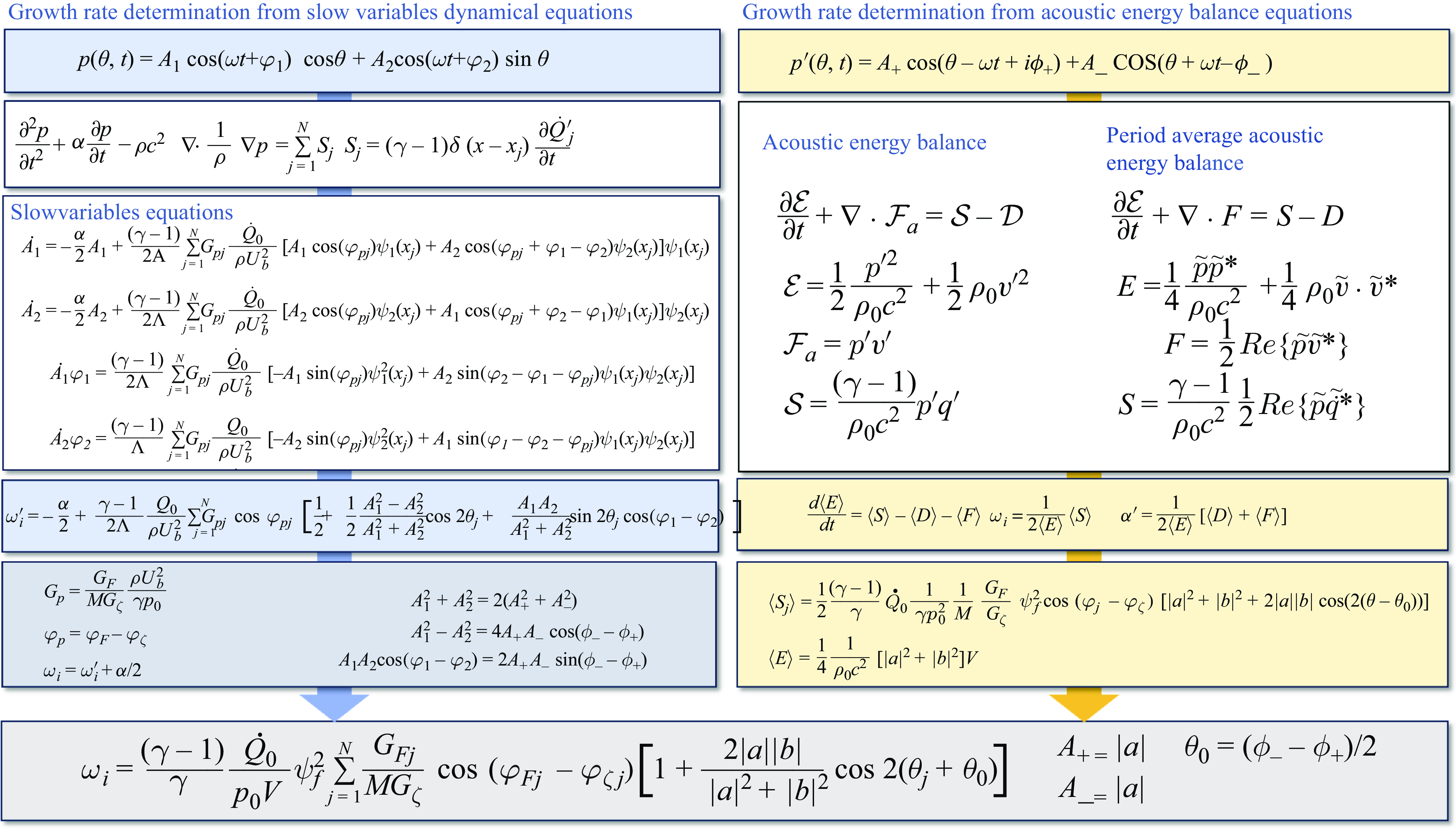
Figure 15. Comparison of two approaches for growth rate determination: slow-flow variable dynamical equations and acoustic energy balance equations.

Figure 16. Effective growth rate
 $\omega^{\prime}_i$
as a function of the number
$\omega^{\prime}_i$
as a function of the number
 $N_S$
of S-injectors (a) and limit-cycle amplitude
$N_S$
of S-injectors (a) and limit-cycle amplitude
 $A(LC)$
as a function of the effective growth rate (b).
$A(LC)$
as a function of the effective growth rate (b).
The growth rate may now be calculated for an oscillation level
 $A=350\,\textrm{Pa}$
(corresponding to the level of fluctuation used for FDF measurements in an externally modulated single-injector configuration in Latour et al. (Reference Latour, Durox, Renaud and Candel2024a
)) using (6.8) and the result is plotted, as a function of the number of S-injectors
$A=350\,\textrm{Pa}$
(corresponding to the level of fluctuation used for FDF measurements in an externally modulated single-injector configuration in Latour et al. (Reference Latour, Durox, Renaud and Candel2024a
)) using (6.8) and the result is plotted, as a function of the number of S-injectors
 $N_S$
for the different configurations investigated, in figure 16(a). The trends found match those calculated in Latour et al. (Reference Latour, Durox, Renaud and Candel2024a
) using a growth rate expression derived from acoustic energy balance equations, and FDF data measured in the weakly nonlinear regime as an input. It is also instructive to plot the limit-cycle oscillation amplitude,
$N_S$
for the different configurations investigated, in figure 16(a). The trends found match those calculated in Latour et al. (Reference Latour, Durox, Renaud and Candel2024a
) using a growth rate expression derived from acoustic energy balance equations, and FDF data measured in the weakly nonlinear regime as an input. It is also instructive to plot the limit-cycle oscillation amplitude,
 $A(LC)$
, as a function of the effective growth rate,
$A(LC)$
, as a function of the effective growth rate,
 $\omega ^{\prime}_i$
, calculated in the linear range (for a low level of oscillation). The corresponding results are shown in figure 16(b). One finds that, the higher the effective growth rate (in the linear range), the higher the limit-cycle oscillation amplitude, a feature that is already present in Latour et al. (Reference Latour, Durox, Renaud and Candel2024a
) (figure 16b of that reference). A quantitative comparison between the growth rates calculated from FDF data in Latour et al. (Reference Latour, Durox, Renaud and Candel2024a
) and the growth rates calculated for a relatively low amplitude level from the slow-flow equations using (6.8) is also provided in figure 17. The growth rates obtained from ODE simulations are higher than those calculated from FDF data, hinting a slight over-prediction of the source term in the weakly nonlinear range with the linear modelling adopted for the HRR.
$\omega ^{\prime}_i$
, calculated in the linear range (for a low level of oscillation). The corresponding results are shown in figure 16(b). One finds that, the higher the effective growth rate (in the linear range), the higher the limit-cycle oscillation amplitude, a feature that is already present in Latour et al. (Reference Latour, Durox, Renaud and Candel2024a
) (figure 16b of that reference). A quantitative comparison between the growth rates calculated from FDF data in Latour et al. (Reference Latour, Durox, Renaud and Candel2024a
) and the growth rates calculated for a relatively low amplitude level from the slow-flow equations using (6.8) is also provided in figure 17. The growth rates obtained from ODE simulations are higher than those calculated from FDF data, hinting a slight over-prediction of the source term in the weakly nonlinear range with the linear modelling adopted for the HRR.
A further examination of the link between the linear growth rate and the amplitude of oscillation at limit cycle is proposed in Appendix E, where an analytical expression is derived by assuming that the coupling involves a standing mode. It is shown that this expression provides limit-cycle amplitudes that follow the trends observed experimentally and yields reasonable estimates of the measured amplitudes.

Figure 17. Comparison between growth rates determined from velocity-based FDF data in Latour et al. (Reference Latour, Durox, Renaud and Candel2024a
) (diamonds) and growth rates deduced from the slow-flow equations in the linear range (circles) for type
 $\mathcal{C}$
(a) and type
$\mathcal{C}$
(a) and type
 $\mathcal{L}$
(b) configurations.
$\mathcal{L}$
(b) configurations.
7. Conclusion
The analysis carried out in this article combines a new technique for controlling the limit-cycle oscillation level in an annular combustor with a theoretical representation of the system’s combustion dynamics in terms of slow-flow variables. This is used to explore the evolution toward the limit cycle, calculate growth rates, determine the level of oscillation and the nature of the coupling mode at limit cycle. It is first shown that pressure-based FDFs may be obtained from well-controlled experiments in an annular combustor by simultaneously recording the pressure and HRR signals under self-sustained oscillations. This is done by controlling the nature of the mode and the limit-cycle oscillation amplitude by mixing two types of injection units leading to different flame dynamics. In particular, the collected experimental data can be used to describe the saturation in the flame response with increasing pressure amplitude levels and obtain an experimentally valid representation of the gain and phase evolution as a function of amplitude. On that basis, it is possible to revisit the theoretical modelling of the flame response to acoustic disturbances and replace current models based on a third-order polynomial description of the HRR fluctuations as a function of the pressure oscillation. In the new model proposed in this work, the flame response, described in terms of HRR fluctuations, appears as a linearly decreasing function of the pressure amplitude level. A generic instability analysis framework is used in a first stage to show that this provides an improved representation of the saturation leading to the limit cycle. This model is used in a second stage as an input in the equations governing the dynamics of an annular combustor as it evolves to a limit cycle. The theoretically predicted limit-cycle oscillation amplitudes using SFVE are compared with experimental data collected in a set of staging experiments carried out in a multiple injector annular combustor MICCA. The model is shown to qualitatively reproduce and quantitatively retrieve experimental observations, in terms of limit-cycle amplitude levels and nature of the modes. There are, admittedly, some differences between calculations and experiments but the general agreement is quite satisfactory. Finally, an expression of the growth rate is extracted from the SFVE, and compared with another expression of that quantity obtained previously by starting from acoustic energy balance principles. The two expressions are found to exactly match, leading to identical growth rate values. It is also demonstrated, perhaps for the first time, that it is possible to predict limit-cycle amplitude levels of instabilities coupled by an azimuthal mode in an annular combustor. This work hence provides a unified framework, bridging results obtained with FDF data obtained in single-injector experiments in the weakly nonlinear range, and flame response modelling, derived from pressure-based FDF measurements under controlled limit-cycle self-sustained oscillations.
Supplementary material
The supplementary material for this article can be found at https://doi.org/10.1017/jfm.2025.10.
Funding
This work is partially supported as part of the France 2030 programme ANR-22-CE05-0022-02 FlySAFe project.
Declaration of interests
The authors report no conflict of interest.
Appendix A. Link between the FDFs based on relative velocity fluctuation and on pressure
The standard FDF uses as input variable the relative velocity fluctucation
 $v^{\prime}/\overline {v}$
and may be defined by
$v^{\prime}/\overline {v}$
and may be defined by
 \begin{equation} \mathcal {F}_v=\frac {{\dot Q}^{\prime}/ {\dot Q}_0}{v^{\prime}/\overline {v}}. \end{equation}
In this article we use an FDF based on pressure defined by
 \begin{equation} \mathcal {F}_p=\frac {{\dot Q}^{\prime}/ {\dot Q}_0}{p^{\prime}/(\rho U_b^2)}. \end{equation}
The velocity and pressure fluctuations acting on the flame may be linked by an effective impedance
 $\zeta$
defined by
$\zeta$
defined by
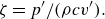 \begin{equation} \zeta = p^{\prime}/(\rho c v^{\prime}) .\end{equation}
Using the previous three expressions one finds that
 \begin{equation} \mathcal {F}_v=\mathcal {F}_p \zeta M \frac {\gamma p_0}{\rho U_b^2}, \end{equation}
where
 $M= \overline {v}/c$
is the Mach number at the flame and where
$M= \overline {v}/c$
is the Mach number at the flame and where
 $ \gamma p_0= \rho c^2$
. It is convenient to introduce the gains and phases of the FDFs and of the effective impedance
$ \gamma p_0= \rho c^2$
. It is convenient to introduce the gains and phases of the FDFs and of the effective impedance
 $\mathcal {F}_v= G_F e^{i\varphi _F}, \, \mathcal {F}_p= G_p e^{i\varphi _p}, \, \zeta = G_\zeta e^{i\varphi _\zeta }$
and deduce
$\mathcal {F}_v= G_F e^{i\varphi _F}, \, \mathcal {F}_p= G_p e^{i\varphi _p}, \, \zeta = G_\zeta e^{i\varphi _\zeta }$
and deduce
 \begin{equation} G_p=\frac {G_F}{MG_\zeta } \frac {\rho U_b^2}{\gamma p_0} \end{equation}
and
 \begin{equation} \varphi _p= \varphi _F-\varphi _\zeta. \end{equation}
As pointed out by a reviewer, the impedance used in this derivation is not purely acoustic, and contains effects, such as shedding and convection of vortical structures. This results from the method used to determine the FDF
 $\mathcal {F}_v$
, which is obtained in Latour et al. (Reference Latour, Durox, Renaud and Candel2024a
) by using velocity fluctuations measured with laser Doppler anemometry (LDA), which does not distinguish purely acoustic velocity fluctuations and velocity disturbances of a different type. The impedance
$\mathcal {F}_v$
, which is obtained in Latour et al. (Reference Latour, Durox, Renaud and Candel2024a
) by using velocity fluctuations measured with laser Doppler anemometry (LDA), which does not distinguish purely acoustic velocity fluctuations and velocity disturbances of a different type. The impedance
 $\zeta$
simply serves to link
$\zeta$
simply serves to link
 $\mathcal {F}_v$
and
$\mathcal {F}_v$
and
 $\mathcal {F}_p$
.
$\mathcal {F}_p$
.
Appendix B. Justification of the assumption
$g^{\prime}(a)a/\omega _0\lt \lt 1$

The easiest way to determine the order of magnitude of
 $g^\prime (a)a/\omega _0$
is to start with the amplitude equation corresponding to a linearly decreasing function
$g^\prime (a)a/\omega _0$
is to start with the amplitude equation corresponding to a linearly decreasing function
 $g(a)$
 \begin{equation} \frac {1}{a}\frac {\textrm{d}\it a}{\textrm{d}\it t} = \frac {1}{2} (g(a)-\alpha ). \end{equation}
One immediately identifies the rate of change of the amplitude on the left-hand side. This is the effective growth rate
 $\omega^{\prime}_i (a)$
. When the amplitude is very small the effective growth rate is
$\omega^{\prime}_i (a)$
. When the amplitude is very small the effective growth rate is
 $\omega^{\prime}_i (0)= (1/2)(g(0) -\alpha )$
and this expression appears on the right-hand side. Now,
$\omega^{\prime}_i (0)= (1/2)(g(0) -\alpha )$
and this expression appears on the right-hand side. Now,
 $|g(a)-g(0)| \ge {max}[g^{\prime}(a) a]$
, and dividing the previous equation by
$|g(a)-g(0)| \ge {max}[g^{\prime}(a) a]$
, and dividing the previous equation by
 $\omega _0$
, one obtains
$\omega _0$
, one obtains
 \begin{equation} \left|\frac {\omega^{\prime}_i(a)-\omega^{\prime}_i(0)}{\omega _0}\right| \ge \frac {1}{2} {max}\left[\frac {g^{\prime}(a)a}{\omega _0}\right] .\end{equation}
Thus
 \begin{equation} {max}\left[\left|\frac {g^{\prime}(a)a}{\omega _0}\right| \right]\le 2 \frac {|\Delta \omega^{\prime}_i|}{\omega _0} \le 2\frac {|\omega^{\prime}_i(0)|}{\omega _0}. \end{equation}
The linear growth rate is typically small compared with the angular frequency of oscillation. In the present experiments
 $\omega^{\prime}_i(0)\simeq 100\, \textrm {s}^{-1}$
while
$\omega^{\prime}_i(0)\simeq 100\, \textrm {s}^{-1}$
while
 $\omega _0 \simeq 2 \pi (800)= 5000\, \textrm {rad s}^{-1}$
so that
$\omega _0 \simeq 2 \pi (800)= 5000\, \textrm {rad s}^{-1}$
so that
 \begin{equation} {max}\left[ \left| \frac {g^{\prime}(a)a}{\omega _0} \right| \right]\lt 0.04 .\end{equation}
The approximate expression of
 $1/\Delta$
is clearly acceptable.
$1/\Delta$
is clearly acceptable.
Appendix C. Normal mode expansion of the pressure field
The derivation of the slow-flow equations relies on an expansion of the pressure field on the set of normal modes of the combustor. The objective of this appendix is to specify the modal eigenfunctions that pertain to the annular geometry of the MICCA combustor, discuss their indexing, determine the value of the normalization constant and briefly explain the method of projection that yields the set of dynamical equations (5.5).
One assumes in what follows that the combustor is annular and that the distance between the lateral walls enclosing the chamber is small compared with the mean radius of the system. In this situation there is no dependence on the radial coordinate and one only needs to consider the axial and azimuthal coordinates
 $x$
and
$x$
and
 $\theta$
. One also assumes that the backplane is rigid like the two sidewalls and that the exhaust is open to the atmosphere. Assuming a constant value for the speed of sound, solutions of the wave equation
$\theta$
. One also assumes that the backplane is rigid like the two sidewalls and that the exhaust is open to the atmosphere. Assuming a constant value for the speed of sound, solutions of the wave equation
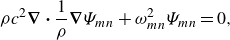 \begin{equation} \rho c^2 \boldsymbol {\nabla } \boldsymbol {\cdot } \frac {1}{\rho }\boldsymbol {\nabla } \Psi _{mn} + \omega _{mn}^2 \Psi _{mn} =0 ,\end{equation}
for the previous boundary conditions may be cast in the form
 \begin{align} \Psi _{mn}^{(1)}(x, \theta )&= \psi _{m}^{||}(x)\cos (n\theta ),\\[-10pt]\nonumber \end{align}
 \begin{align} \Psi _{mn}^{(2)}(x,\theta )&= \psi _{m}^{||}(x)\sin (n\theta ) .\end{align}
In these expressions
 $\psi _{m}^{||}(x)$
represent the axial wave function of order
$\psi _{m}^{||}(x)$
represent the axial wave function of order
 $m$
,
$m$
,
 $\psi _{m}^{||}(x)= \cos [m\pi x/(2 l)]$
while
$\psi _{m}^{||}(x)= \cos [m\pi x/(2 l)]$
while
 $\cos (n\theta )$
and
$\cos (n\theta )$
and
 $\sin (n\theta )$
designate the azimuthal wave functions of order
$\sin (n\theta )$
designate the azimuthal wave functions of order
 $n$
. For a given eigenvalue
$n$
. For a given eigenvalue
 $\omega _{mn}$
, there are two independent modes in the azimuthal direction that correspond to the cosine and sine functions. It is convenient to use an index
$\omega _{mn}$
, there are two independent modes in the azimuthal direction that correspond to the cosine and sine functions. It is convenient to use an index
 $\nu =1, \, \textrm {or}\, 2$
to distinguish these two functions. The pressure field may be expanded over this double set of normal modes
$\nu =1, \, \textrm {or}\, 2$
to distinguish these two functions. The pressure field may be expanded over this double set of normal modes
 \begin{equation} p(x, \theta ,t) = \sum _{mn} {{\eta _{mn}}^{(1)}}(t) \Psi _{mn}^{(1)} + \sum _{mn}{{\eta _{mn}}^{(2)}}(t) \Psi _{mn}^{(2)} .\end{equation}
It is a simple matter to show that the normal modes
 $\Psi _{mn}^{(\nu )}$
form an orthogonal basis and to determine the normalization constant
$\Psi _{mn}^{(\nu )}$
form an orthogonal basis and to determine the normalization constant
 \begin{equation} \Lambda ^{\nu }_{mn}= \int _V [\Psi _{mn}^{(\nu )}]^2 \textrm{d}\it V .\end{equation}
For modes that have an azimuthal number
 $n$
that is non-zero, one finds that
$n$
that is non-zero, one finds that
 $\Lambda ^{\nu }_{mn}= (1/4)V$
and this common value will be designated by
$\Lambda ^{\nu }_{mn}= (1/4)V$
and this common value will be designated by
 $\Lambda$
. Purely axial modes (
$\Lambda$
. Purely axial modes (
 $n=0$
) feature a normalization constant
$n=0$
) feature a normalization constant
 $\Lambda _{m0}= (1/2) V$
but these modes are not considered in the present analysis. The pressure field expansion may be introduced in the wave equation (5.1) which is then projected on the mode
$\Lambda _{m0}= (1/2) V$
but these modes are not considered in the present analysis. The pressure field expansion may be introduced in the wave equation (5.1) which is then projected on the mode
 $\Psi _{mn}^{(\nu )}$
. This yields
$\Psi _{mn}^{(\nu )}$
. This yields
 \begin{equation} {\ddot \eta }_{mn}^\nu +\alpha {\dot \eta }_{mn}^\nu + \omega ^2_{mn}{\eta }_{mn}^\nu =\frac { 1} {\Lambda _{mn}^\nu } \int _V S \Psi _{mn}^\nu \textrm{d}\it V \, \, \textrm {for} \,\, \nu =1,2 .\end{equation}
The dynamical equations are here derived by considering the 1A1L mode, i.e. the first azimuthal
 $n=1$
, first longitudinal
$n=1$
, first longitudinal
 $m=1$
mode. In the analysis we also assume that the flames act like point sources located at an axial distance
$m=1$
mode. In the analysis we also assume that the flames act like point sources located at an axial distance
 $x_f$
from the backplane and at azimuthal angles
$x_f$
from the backplane and at azimuthal angles
 $\theta _j, \,\, j=1,\ldots, N$
so that the axial eigenfunction is evaluated at that distance. It is then convenient to set
$\theta _j, \,\, j=1,\ldots, N$
so that the axial eigenfunction is evaluated at that distance. It is then convenient to set
 $\psi _f= \psi _{1}^{||}(x_f)$
and write the pressure field acting on the flames in the form
$\psi _f= \psi _{1}^{||}(x_f)$
and write the pressure field acting on the flames in the form
 \begin{equation} p(x_f, \theta , t) = \psi _f [\eta ^{(1)}_{11} (t) \cos \theta + \eta ^{(2)}_{11} (t) \sin \theta ] .\end{equation}
The notation can simplified by replacing the previous expression by
 \begin{equation} p(x_f, \theta , t) = \psi _f [\eta _{1} (t) \cos \theta + \eta _2 (t) \sin \theta ] .\end{equation}
The two modal amplitudes then satisfy the set of differential equations (5.5).
Appendix D. Relation between the standing modes amplitudes
$A_1$
and
$A_2$
and the azimuthal wave amplitudes
$A_+$
and
$A_-$


It is useful to establish links between the present representation of the pressure field
 \begin{equation} p^{\prime}(\theta , t)= A_1 \cos (\omega t+ \varphi _1) \cos \theta + A_2 \cos ((\omega t+ \varphi _2)\sin \theta \end{equation}
and the standard formulation of this field in the form of a sum of two azimuthal waves
 \begin{align} p^{\prime}(\theta , t)&= Re\{A_+\exp (i\theta -i\omega t + i \phi _+) + A_-\exp (-i\theta -i\omega t + i \phi _-)\} \\[-10pt]\nonumber\end{align}
 \begin{align} &= A_+ \cos ( \theta -\omega t + \phi _+) + A_-\cos (\theta + \omega t - \phi _-) .\end{align}
By matching these two representations one finds that
 \begin{align} A_+ \cos (\omega t-\phi _+) + A_-\cos (\omega t - \phi _-)&= A_1 \cos (\omega t + \varphi _1),\end{align}
 \begin{align} A_+ \sin (\omega t-\phi _+) - A_-\sin (\omega t - \phi _-)&= A_2 \cos (\omega t + \varphi _2) .\end{align}
One may then deduce a complex versions of these two expressions
 \begin{align} A_+ e^{i\phi _+} +A_{-}e^{i\phi _-}&= A_1 e^{-i\varphi _1} ,\end{align}
 \begin{align} A_+ e^{i\phi _{+} + i \pi /2} - A_{-}e^{i\phi _{-}+i \pi /2} &= A_2 e^{-i\varphi _2} .\end{align}
Multiplying these two expressions by their complex conjugates, and multiplying the first by the complex conjugate of the second one obtains
 \begin{align} &A_1^2 = A_+^2 + A_-^2 + 2 A_+ A_- \cos (\phi _- -\phi _+) ,\end{align}
 \begin{align} &A_2^2 = A_+^2 + A_-^2 -2 A_+ A_- \cos (\phi _- -\phi _+),\end{align}
 \begin{align} A_1A_2 \cos (\varphi _1-\varphi _2)= 2 A_+A_- \sin (\phi _- -\phi _+) .\end{align}
It is then easy to deduce the following set of expressions:
 \begin{align} A_1^2 +A_2^2 & = 2(A_+^2 + A_-^2), \end{align}
 \begin{align} A_1^2 -A_2^2 &= 4 A_+ A_- \cos (\phi _- -\phi _+), \end{align}
 \begin{align} A_1A_2 \cos (\varphi _1-\varphi _2)&= 2 A_+A_- \sin (\phi _- -\phi _+),\end{align}
 \begin{align} A_1A_2 \sin (\varphi _1-\varphi _2)&= A_+^2-A_-^2 .\end{align}
These expressions can then be used to write the growth rate
 $\omega _i$
in terms of the azimuthal wave amplitudes
$\omega _i$
in terms of the azimuthal wave amplitudes
 $A_+, A_-$
and phases
$A_+, A_-$
and phases
 $\phi _+, \phi _-$
(see § 5). It is also a simple matter to link
$\phi _+, \phi _-$
(see § 5). It is also a simple matter to link
 $\varphi _1-\varphi _2$
and
$\varphi _1-\varphi _2$
and
 $\theta _0$
. Some calculations yield
$\theta _0$
. Some calculations yield
 \begin{equation} \tan (2 \theta _0) = \frac { 2 A_1A_2}{A_1^2 -A_2^2} \cos (\varphi _1-\varphi _2). \end{equation}
Nevertheless, care has to be taken to ensure that the correct value of
 $\theta _0$
is obtained.
$\theta _0$
is obtained.
Using
 \begin{equation} \sin (2 \theta _0) = \frac {2A_1A_2 \cos (\varphi _1-\varphi _2)}{[\big(A_1^2+A_2^2\big)^2 - 4 A_1^2A_2^2 \sin ^2(\varphi _1-\varphi _2)]^{1/2}} \end{equation}
and
 \begin{equation} \cos (2 \theta _0) = \frac {A_1^2-A_2^2}{[\big(A_1^2+A_2^2\big)^2 - 4 A_1^2A_2^2 \sin ^2(\varphi _1-\varphi _2)]^{1/2}} ,\end{equation}
one gets the following expression, ensuring that
 $\theta _0$
is always defined in the
$\theta _0$
is always defined in the
 $[-\pi /2, \pi /2]$
range:
$[-\pi /2, \pi /2]$
range:
 \begin{equation} \theta _0 = \tfrac {1}{2} {sign} \{\sin 2 \theta _0 \} \cos ^{-1} [\cos 2 \theta _0]. \end{equation}
It is also interesting to express the spin ratio as a function of the amplitudes
 $A_1, A_2$
and phases
$A_1, A_2$
and phases
 $\varphi _1, \varphi _2$
. The spin ratio is defined by
$\varphi _1, \varphi _2$
. The spin ratio is defined by
 $s_r= (A_+ -A_-)/(A_{+} +A_{-})$
which may also be written as
$s_r= (A_+ -A_-)/(A_{+} +A_{-})$
which may also be written as
 $s_r= (A_+^2 - A_-^2)/ (A_+^2+ A_-^2 + 2A_+A_-)$
. Using expressions (D11) to (D14) one may write
$s_r= (A_+^2 - A_-^2)/ (A_+^2+ A_-^2 + 2A_+A_-)$
. Using expressions (D11) to (D14) one may write
 \begin{equation} s_r=\frac {A_1A_2 \sin (\varphi _1-\varphi _2)}{(1/2)\big(A_1^2+A_2^2\big) + (1/2)(A_1^2-A_2^2)/ \cos 2\theta _0}, \end{equation}
which becomes after some algebra
 \begin{equation} s_r=\frac {A_1A_2 \sin (\varphi _1-\varphi _2)\cos 2\theta _0}{(A_1^2\cos ^2\theta _0-A_2^2\sin ^2\theta _0) } .\end{equation}
Appendix E. Analytical expression of the limit-cycle oscillation amplitude
An analytical expression of the limit-cycle amplitude may be derived from the general expression of the growth rate by making use of some simplifying assumptions. In what follows we consider two families of injectors designated by U and S and assume that the gain of the pressure based describing function is a linear function of the reduced r.m.s. pressure
 $\Pi _j = (p^{\prime}_j)_{rms}/\rho U_b^2$
so that one can write
$\Pi _j = (p^{\prime}_j)_{rms}/\rho U_b^2$
so that one can write
 \begin{align} G_{p_j}^U&= \beta ^U -\kappa ^U \Pi _j ,\end{align}
 \begin{align} G_{p_j}^S&= \beta ^S -\kappa ^S \Pi _j .\end{align}
It is also assumed, for the sake of simplicity, that the phases of the pressure based describing function do not change with the amplitude
 $\Pi _j$
so that one may use constant values for the phases
$\Pi _j$
so that one may use constant values for the phases
 $\varphi _j^U=\varphi ^U$
and
$\varphi _j^U=\varphi ^U$
and
 $\varphi _j^S=\varphi ^S$
. The present calculations are carried out by assuming that the coupling is induced by a standing mode. This is the case for example in configurations
$\varphi _j^S=\varphi ^S$
. The present calculations are carried out by assuming that the coupling is induced by a standing mode. This is the case for example in configurations
 $\mathcal {C}_4, \mathcal {C}_6$
and
$\mathcal {C}_4, \mathcal {C}_6$
and
 $\mathcal {L}_2, \mathcal {L}_4, \mathcal {L}_6, \mathcal {L}_8$
. The growth rate may then be written in the form
$\mathcal {L}_2, \mathcal {L}_4, \mathcal {L}_6, \mathcal {L}_8$
. The growth rate may then be written in the form
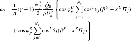 \begin{align} \omega _i & = \frac {1}{\Lambda }(\gamma -1)\frac {\psi _f^2}{2}\frac {{\dot Q}_0}{\rho U_b^2}\left\{ \cos \varphi _p^U \sum _{j=1}^{N_u} \cos ^2 \theta _j (\beta ^U- \kappa ^U\Pi _j)\right.\nonumber\\& \quad \left. + \cos \varphi _p^S \sum _{j=1}^{N_s} \cos ^2 \theta _j (\beta ^S- \kappa ^S\Pi _j) \right\} .\end{align}
It is possible to identify in this expression the linear growth rate corresponding to low amplitude levels
 $\omega _i(0)$
and another term
$\omega _i(0)$
and another term
 $\chi$
that defines the change in
$\chi$
that defines the change in
 $\omega _i$
due to the growth of oscillation amplitude. One may thus write
$\omega _i$
due to the growth of oscillation amplitude. One may thus write
 \begin{equation} \omega _i = \omega _i(0) -\chi ,\end{equation}
where
 \begin{align} \omega _i(0) & =\omega _i^U(0)\Big \{1- \frac {\beta ^U \cos \varphi _p^U-\beta ^S\cos \varphi _p^S}{\beta ^U\cos \varphi _p^U}\frac {2}{N}\sum _{j=1}^{N_s} \cos ^2 \theta _j \Big \}, \end{align}
 \begin{align} \chi &=\omega _i^U(0) \frac {\kappa ^U}{\beta ^U} \Big \{\frac {8}{3\pi }- \frac {\kappa ^U \cos \varphi _p^U-\kappa ^S\cos \varphi _p^S}{\kappa ^U\cos \varphi _p^U}\frac {2}{N}\sum _{j=1}^{N_s} \cos ^2 \theta _j |\cos \theta _j| \Big \}\Pi _{max} ,\end{align}
where
 \begin{equation} \omega _i^U(0) = (\gamma -1) \psi _f^2 \frac {{\dot Q}_0 N}{\rho U_b^2 V}\cos \varphi _p^U \beta ^U \end{equation}
designates the linear growth rate when all injectors are of the U-type, and
 \begin{equation} \Pi _{max}=\frac {a}{2^{1/2}} \frac {1}{\rho U_b^2} \psi _f \end{equation}
represents the maximum value of the reduced r.m.s. pressure level. It is convenient to define a parameter
 $C$
such that
$C$
such that
 \begin{equation} C=\left\{\frac {8}{3\pi }- \frac {\kappa ^U \cos \varphi _p^U-\kappa ^S\cos \varphi _p^S}{\kappa ^U\cos \varphi _p^U}\frac {2}{N}\sum _{j=1}^{N_s} \cos ^2 \theta _j |\cos \theta _j| \right\} .\end{equation}
With these definitions one may now express the growth rate in the following form:
 \begin{equation} \omega _i= \omega _i(0)-\omega _i^U(0) C \Pi _{max} .\end{equation}
When all injectors are of the U-type,
 $C= 8/(3\pi )$
. When the number
$C= 8/(3\pi )$
. When the number
 $N_s$
is small and all S injectors are located near the pressure nodal line
$N_s$
is small and all S injectors are located near the pressure nodal line
 $C\simeq 8/(3\pi )$
and one may also use that expression. In the more general case, one has to calculate
$C\simeq 8/(3\pi )$
and one may also use that expression. In the more general case, one has to calculate
 $C$
.
$C$
.
It is now easy to determine the value of
 $\Pi _{max}$
at the limit cycle. This can be done by noting that at the limit cycle
$\Pi _{max}$
at the limit cycle. This can be done by noting that at the limit cycle
 $\omega _i = \alpha$
so that
$\omega _i = \alpha$
so that
 \begin{equation} \Pi _{max}(lc)=\frac {\omega _i(0)-\alpha }{C(\kappa ^U/{\beta ^U})\omega _i^U(0)} .\end{equation}
One obtains
 \begin{equation} \frac {a}{2^{1/2}}=\frac { \beta ^U}{\kappa ^U}\frac {\omega _i(0)-\alpha }{C\omega _i^U(0)\psi _f}\rho U_b^2 .\end{equation}
The previous expressions feature a linear dependence of the limit-cycle amplitude with respect to the effective growth rate
 $\omega ^{\prime}_i$
. They can be used to predict the r.m.s. pressure level at the limit cycle
$\omega ^{\prime}_i$
. They can be used to predict the r.m.s. pressure level at the limit cycle
 $a/2^{1/2}$
and compare this value with
$a/2^{1/2}$
and compare this value with
 $A$
determined experimentally. Table 3 gathers predicted values and experimental data for the injector arrangements corresponding to a coupling by a standing mode. One can see that the trends (lower amplitude values for type
$A$
determined experimentally. Table 3 gathers predicted values and experimental data for the injector arrangements corresponding to a coupling by a standing mode. One can see that the trends (lower amplitude values for type
 $\mathcal{C}$
than type
$\mathcal{C}$
than type
 $\mathcal{L}$
configurations) are correctly retrieved. A good match is observed between the model’s predictions and the experimental data, and, as for the limit-cycle amplitudes obtained by solving the slow-flow variables ODEs (see § 5), larger discrepancies are observed between experimental data and model prediction for type
$\mathcal{L}$
configurations) are correctly retrieved. A good match is observed between the model’s predictions and the experimental data, and, as for the limit-cycle amplitudes obtained by solving the slow-flow variables ODEs (see § 5), larger discrepancies are observed between experimental data and model prediction for type
 $\mathcal{L}$
than for type
$\mathcal{L}$
than for type
 $\mathcal{C}$
configurations.
$\mathcal{C}$
configurations.
Table 3. Comparison between the experimental limit-cycle amplitudes,
 $A$
, and the values estimated from the analytical model.
$A$
, and the values estimated from the analytical model.


