1 Introduction
After the 2008 global financial crisis, the performance of US pension funds has remained depressed. The poor solvency situation has been driven by a declining discount rate and also a fall in equity prices. Since 2012, funding ratios (asset values divided by projected benefit obligations) of the top 100 largest US corporate defined-benefit pension plans have not rebounded. More importantly, projected future funding ratios show a wide range of uncertainty for the next 2 years.Footnote 1 This raises the question of how to price and hedge downside risks when confronted with fragile beliefs about the likelihood of different funding ratio scenarios.
Pricing and hedging pension or insurance liabilities faces two problems. First, the market is incomplete. Liability risks are typically not – or not actively – traded in the financial market. According to EIOPA (Reference EIOPA2011)Footnote 2, the two largest components of liability risks are market risk and life risk, which account for 67.4% and 23.7% of the diversified Basic Solvency Capital Requirement (SCR), respectively. However, these risks are not fully traded. Interest rate risk, one of the dominant market risks, is only partially traded in the financial market. Pension funds and insurance companies are often confronted with ultra-long-term commitments with maturities of more than 50 years. However, the longest dated government bonds even in developed markets such as the US, UK, and Canada are up to 30 years. In developing markets (such as Asia, Eastern Europe, and South America), long-term government bonds with maturities more than 10 years barely exist.
Life risk faces more serious market incompleteness problem, because mortality-linked securities in general have very low liquidity. For instance, longevity risk, the risk that insurers might live longer than anticipated, is the most important component of life risk. Turner (Reference Turner2006) shows that, in 2005,  ${\rm \pounds}$ 2460 billion liabilities are associated with longevity risk in the UK. However, longevity risk had never been securitized until early 2000s. In the past decade, a limited number of mortality-linked products such as the longevity bond (see Blake and Burrows (Reference Blake and Burrows2001)) have been proposed, while only a very small amount (<1%Footnote 3) of longevity risk can be hedged.
The second problem concerns model parameter uncertainty in hedging liability risks. On the liability side of the balance sheet, longevity has been improving unprecedentedly in the past few decades in an unpredictable way (see, e.g. Benjamin and Soliman, Reference Benjamin and Soliman1993; McDonald et al., Reference McDonald, Cassano and Fahlenbrach2006). An inaccurate mortality estimation makes pricing and hedging liability risks much more difficult and less reliable. Early work by Lee and Carter (Reference Lee and Carter1992) has been considered as the nucleus of modeling the dynamics of the mortality rate. Several plausible extensions of the Lee–Carter model, such as an incorporation of heterogeneous cell level (Li et al., Reference Li, Hardy and Tan2009), age-dependent factors (Cairns et al., Reference Cairns, Blake and Dowd2006), and structural changes (Coelho and Nunes, Reference Coelho and Nunes2011; Van Berkum et al., Reference Van Berkum, Antonio and Vellekoop2016), introduce substantial uncertainty on the trend in longevity and hence in the growth in liabilities.
On the other side of the balance sheet, the expected asset return is notoriously difficult to estimate from historical data. Merton (Reference Merton1980) argues that it is difficult to estimate expected returns from time series of realized stock return data. The standard deviation of the historical average return is  $\sigma /\sqrt T $ where σ is the standard deviation of annual returns and T is the number of years. For example, if T = 100 and
  $\sigma = 16\% $, then the standard error of the equity premium is 1.6%, which leads to an approximate 95% confidence interval span of
  $6.3\% ( \pm 1.96 \times 1.6\% )$. Although the interval shrinks with the square root of the sample size for estimation, it is difficult to maintain the same data generating process throughout the entire period. The investor is therefore exposed to estimation error in the expected asset returns.
Doubts about the accuracy of the model makes an agent treat it as an approximation of an unknown true model. She wants her decision rules to work well over a set of models in the neighborhood of the approximating model. Our aim is to develop a hedging strategy for an agent who faces uncertainty about the expected return on the assets as well as uncertainty about the expected growth in liabilities. We adopted the robust control theory to deal with the fear of model uncertainty. The agent who worries about model misspecification looks for a prudent policy that is resilient to fragile beliefs about the likelihood of the state variables. Such decision rules are called robust policies. We introduced a robust hedging strategy along the lines of Hansen and Sargent (Reference Hansen and Sargent2007) to hedge undiversifiable downside risks.
The robust optimal hedging strategy that we propose takes both downside risks as well as market incompleteness into account for an agent who fears parameter uncertainty. The robust agent is assumed to minimize the shortfall between assets and liabilities under a statistically plausible worst-case scenario by means of solving a min–max robust optimization problem. The robust model includes three crucial elements. The first is downside risk, which we define as expected shortfall. In a static model, the expected shortfall between the assets and the liabilities can be valued as the payoff of an exchange option, which swaps the optimal value of the asset for the price of the liabilities. The second element is incomplete markets. We introduced two uncorrelated risk drivers in our model, one hedgeable and the other not hedgeable. The unhedgeable risk captures the incompleteness of the market. The asset market is exposed to hedgeable risk only, but the liability side is exposed to both types of risk. The third element is parameter misspecification. Following Anderson et al. (Reference Anderson, Hansen and Sargent2003) and Maenhout (Reference Maenhout2004), we introduced drift distortions on the Brownian motions to represent parameter misspecification. These drift distortions perturb the true data generation process of approximate models. Economically, an additional drift on the Brownian motion can be understood as the unobservable market price of risk, which relates to Cochrane and Saa-Requejo (Reference Cochrane and Saa-Requejo2000)’s concept of Good Deal Bounds (GDB). Technically, drift distortions measure the discrepancies between alternative probability distributions. A closely related idea appears in Cvitanić and Karatzas (Reference Cvitanić and Karatzas1999), but in their model, liabilities only depend on the value of market instruments.
We solved the robust hedging problem in both a static and a dynamic environment. In both cases, the robust policy is more conservative than the naive policy. This result is in line with Brennan (Reference Brennan1998). When the funding ratio is low, agents will increase the risk exposure to the stock market so as to gamble their way out of trouble (see also Ang et al., Reference Ang, Chen and Sundaresan2013). The more the investor invests in the risky asset, the more she becomes exposed to estimation uncertainty. The robust agent is particularly afraid of a downside shock with the risky assets and hence she will put less wealth in the stock market compared with the agent who disregards the estimation uncertainty. We also found that for both the robust as well as the non-robust policy, the risky portion of the portfolio decreases with the hedging horizon when the funding ratio is low, and vice versa when the funding ratio is high. The impact of the preference for robustness depends on the hedging horizon as well as the funding ratio.
More importantly, we evaluated the robust policy by means of comparing its expected loss with the non-robust policy. The loss function is defined as the difference between the cost of hedging conditional on the estimated expected return and the true minimum cost. The benefits of a robust policy are twofold. First, the robust policy is less sensitive to the estimated parameters. Second, the robust policy has a lower hedging cost than a naive policy, under a range of alternative parameter values.
One strong assumption in this paper is that the investors only fear a subclass of model misspecification, namely the drift parameters of the state variables instead of the general model uncertainty problem. Similar to Maenhout (Reference Maenhout2004), we reduced the general model uncertainty problem to a first-moment parameter uncertainty problem.
Another strong assumption in our work is that the investors do not engage in any learning. Brennan (Reference Brennan1998) incorporates learning with parameter uncertainty and finds that after learning, high-risk-averse investors are more conservative with their investment, but low-risk-averse investors allocate more wealth on risky assets. Wang (Reference Wang2009) incorporates income growth rate uncertainty with Bayesian learning for a consumption-saving and optimal portfolio choice problem and finds that learning induces additional precautionary saving.
Numerous studies deal with asset allocation problem for pension plans. Seminal work by Sharpe and Tint (Reference Sharpe and Tint1990) develops a surplus management approach in which funds care about assets minus liabilities. Detemple and Rindisbacher (Reference Detemple and Rindisbacher2008) extend this framework to a dynamic setting. Ang et al. (Reference Ang, Chen and Sundaresan2013) add an additional penalty function at the mean-variance framework of Sharpe and Tint (Reference Sharpe and Tint1990). The penalty function, which is the shortfall between the asset and liabilities, is the same as our objective function, to which we add model uncertainty.
A related study on model uncertainty by Garlappi et al. (Reference Garlappi, Uppal and Wang2006) considers a mean-variance portfolio choice of a robust investor who has imperfect information on the expected return. They use multi-prior approach advocated by Gilboa and Schmeidler (Reference Gilboa and Schmeidler1989), and they also find that allowing for parameter uncertainty reduces the portfolio weights on risky assets over time. Luo (Reference Luo2016) considers both model uncertainty and state uncertainty under decision-making. State uncertainty refers to incomplete information about the true value of the state due to sluggishness of the market. In this paper, we do not deal with state uncertainty, but the likelihood over the state variables.
2 Model
We considered a continuous-time incomplete market with a finite trading horizon [0, T]. The risk is modeled by a filtered probability space  $(\Omega, {\rm {\cal F}},{\opf P})$, on which are defined two uncorrelated risk factors, a hedgeable risk W 1t and an unhedgeable risk W 2t. Both W 1t and W 2t are univariate standard Brownian motions and we considered
  $\{ {\rm {\cal F}}_t:t \in \left[ {0,T} \right]\} $ as the completion of the filtration generated by W 1t and W 2t. A hedgeable risk means we can replicate the payoff of this kind of risk perfectly. The payoff for an unhedgeable risk is not replicable because it is not traded.
2.1 Asset and liability model
On the asset side, we have a risk-free money-market account B t, which earns a deterministic risk-free rate of interest r, so dB t = rB tdt. We also have a stock market. The stock price follows a geometric Brownian motion process  $dS_t = \mu S_t dt + \sigma S_t dW_{1t}$. The agent can only invest in the money-market account and the stock market. Denote the value of the assets at time t by A t. The investor puts an amount w tA t in the stock market at time t. The remaining part of the assets (1 − w t)A t is put into the money-market account. The asset diffusion process follows as
 $$dA_t = (r + w_t(\mu - r)) A_t dt + w_t \sigma A_t dW_{1t},$$
where w t is the possibly time-varying hedging strategy. We do not set a constraint on w t, therefore short positions are allowed.
The liability is exposed to both hedgeable risk W 1t and unhedgeable risk W 2t. We assumed that the diffusion process of the liability L t follows an exogenously given geometric Brownian motion with constant drift term and constant volatility,
 $$dL_t = a L_t dt + b L_t \left( {\rho dW_{1t} + \sqrt {1 - \rho ^2} dW_{2t}} \right),$$
where a is the drift of the liability and b is its volatility. The non-traded risk driver, dW 2t, represents the incomplete part of the market. We introduced a correlation parameter ρ ∈ [−1, 1] between asset risk and liability risk. It controls the risk exposure to W 2t of the liability. If ρ = ±1, then the non-traded risk W 2t disappears from the liability side. The liability in this case can be perfectly hedged by a replicating portfolio. We are interested in the case when ρ is strictly between −1 and 1.
2.2 Robust asset and liability model
We used the Hansen and Sargent's (Reference Hansen and Sargent2007) framework to integrate the preference for robustness to the asset-liability models (1) and (2). With a preference for robustness, the agent treats (1) and (2) as an approximate model for the unknown true state evolution of A t and L t. We limited the parameter uncertainty to the drift terms μ and a only, and assumed that the volatilities σ and b are known. The approximate model only provides an estimated value of the drift terms, but the growth rate of liabilities and the expected return are imprecisely estimated and subject to estimation error. However, the constant volatility parameter σ can potentially be estimated using high-frequency observations, and is therefore not subject to parameter estimation error.
In the Hansen and Sargent's framework, the robust model contains an unknown drift term on the Brownian motion. In our case, the Brownian motions dW 1t and dW 2t in (1) and (2) are replaced by dW 1t + λ 1tdt and dW 2t + λ 2tdt. The two drift terms λ 1t and λ 2t are defined as two perturbation time-series processes that quantify the misspecification of the underlying model. The values of λ 1t and λ 2t shift the mean distribution of the asset and the liability diffusion process by a unit of w tσλ 1t and  $b\rho \lambda _{1t} + b\sqrt {1 - \rho ^2} \lambda _{2t}$, respectively. Hence, they specify a set of alternative measures referring to different specifications of the stochastic process known as a Girsanov kernel. The misspecified expected return also generates an error in the market price of risk. The perturbed evolution of the state variables is given by:
 $$dA_t = (r + w_t(\mu - r)) A_t dt + w_t\sigma A_t \left({dW_{1t} + \lambda _{1t}dt}\right),$$
 $$dL_t = a L_t dt + b L_t \left( {\rho \left( {dW_{1t} + \lambda _{1t}dt} \right) + \sqrt {1 - \rho ^2} \left( {dW_{2t} + \lambda _{2t}dt} \right)} \right).$$
The perturbation of the model is bounded by an uncertainty set  ${\opf S}$. The larger the uncertainty set
  ${\opf {S}}$, the more pessimistic the agent is about the accuracy of the underlying model. To describe the uncertainty set, we introduced some additional notation. Let δ be the vector of the estimated drift terms,
 $$\delta = \left( {\matrix{ \mu \cr a \cr}} \right)$$
and let δ 0 be the true drift. Then δ − δ 0 is the estimation error,
 $$\delta - \delta _0 = \left( {\matrix{ \sigma & 0 \cr {b\rho} & {b\sqrt {1 - \rho ^2}} \cr}} \right)\left( {\matrix{ {\lambda _{1t}} \cr {\lambda _{2t}} \cr}} \right) = \Gamma \lambda _t.$$
The estimation error δ − δ 0 is asymptotically normal with mean zero and covariance matrix (Σ/N), where N is the length of a (hypothetical) sample used for estimation and  $\Sigma = \Gamma {\Gamma} ^{\prime} = \left( {\matrix{ {\sigma ^2} & {b\rho \sigma} \cr {b\rho \sigma} & {b^2} \cr}} \right)$.
We obtained the uncertainty set based on the property that (δ − δ 0)′(Σ/N)−1(δ − δ 0) is a χ 2 distribution with two degrees of freedom, χ 2(2). Denoting the critical value at α significance level as CVα, we then have a probability of 1 − α that
 $$\left( {\delta - \delta _0} \right)^{\prime}\Sigma ^{ - 1}\left( {\delta - \delta _0} \right) \le \kappa ^2,$$
where κ 2 = (CVα/N). Equation (4) provides a natural boundary of the perturbation parameters. Simplifying (4) further, we get
 $$\left( {\Gamma \lambda _t} \right)^{\prime}\left( {\Gamma {\Gamma} ^{\prime}} \right)^{ - 1}\left( {\Gamma \lambda _t} \right) = {\lambda} ^{\prime}_t\lambda _t \le \kappa ^2.$$
Hence our uncertainty set is as follows,
 $${\opf S} = \left\{ {\lambda _{1t},\lambda _{2t} \vert \lambda _{1t}^2 + \lambda _{2t}^2 \le \kappa ^2} \right\}.$$
Our uncertainty set has a circular shape in λ t space centered by zero. Given the estimates δ a credibility region for the true value, δ 0 can be constructed as
 $$\delta_0 \in \left\{{\delta + \Gamma \lambda_t \vert {\opf S}} \right\}.$$
The true drift term δ 0 is constrained by an ellipsoid uncertainty set centered by δ and it can be at any point within this set. The size of the uncertainty set depends on the significance level α and the hypothetical sample size N. If the agent has infinite observations, then the uncertainty set shrinks to the point estimate δ.
Our stylized uncertainty set is related to the GDB proposed by Cochrane and Saa-Requejo (Reference Cochrane and Saa-Requejo2000). Equation (4) can be understood as the GDB constraint in which we put a limit on the unobservable part of the market price of risks, λ 1t and λ 2t. The uncertainty set we proposed differs from the GDB in the way in which our uncertainty set is derived from the econometric estimation error. The uncertainty set parameter κ depends only on the statistical quantities, α and N. However, the GDB method is inspired by an economic belief that the total market price of risk in an incomplete market has to have limits.
2.3 Robust optimization problem
Utility is defined as a function of the terminal value for A T and L T at the terminal date T. The optimal hedging strategy maximizes the utility function  ${\rm {\opf E}}[U(A_T, L_T)\vert{\rm {\cal F}}_t]$. As a benchmark, we defined the naive policy w na as the hedging strategy that does not consider model misspecification.
The uncertainty averse agent looks for a robust hedging policy that works well over a set of models. The robust hedging policy is defined as
 $$\mathop {\max} \limits_{w_t} \mathop {\min} \limits_{\lambda _{1t},\lambda _{2t} \in {\opf S}} {\rm {\opf E}}\left[ {U\left( {A_T, L_T} \right) \vert {\rm {\cal F}}_t} \right].$$
The max–min optimization problem is a two-player zero-sum game, see Anderson et al. (Reference Anderson, Hansen and Sargent2003). This is a sequential game between the decision-maker and a malevolent nature. Player 1, the robust agent moves first by choosing investment decisions to maximize the utility function at time t, and then player 2 (the imaginary nature) picks the worst state of nature for player 1 by making an instantaneous choice of λ 1t and λ 2t, given player 1's choice. In other words, the agent is maximizing while nature is minimizing.
3 Static robust optimization
In the following two sections, we will show how to solve the robust optimization problem and how the robust solution differs from the naive one, and also how we can benefit from the robust decision. We started with the relatively simple static case, where both agent and nature only make decisions now at t = 0 without rebalancing until the terminal date T. The static case is technically easy to solve, but still provides us with some intuition about the robust policy. However, the static solution may not be optimal. With a dynamic solution both w t and λ 1t, λ 2t are time-series processes.
Given the information at time T, our hedging strategy is defined over the hedging error L T − A T at a predetermined time T. Our utility function takes the form of the shortfall risk  $U\left( {A_T, L_T} \right) = - \left[ {L_T - A_T} \right]^ + $, which specifies the downside risk on the liability shortfall. The lower the shortfall risk, the higher the agent's utility will be. The naive optimization problem is given by
 $$\mathop {\min} \limits_{w_t} {\rm {\opf E}}[(L_T - A_T)^ + ]$$
and the robust optimization is
 $$\mathop {\min} \limits_{w_t} \mathop {\max} \limits_{\lambda _{1t},\lambda _{2t} \in {\opf S}} {\rm {\opf E}}[(L_T - A_T)^ + ].$$
In the static case, the order of the two players is interchangeable. According to the saddle-point existence Theorem mentioned in Delbaen (Reference Delbaen2002) and Rockafellar (Reference Rockafellar1976), the optimal solution of (9) is a saddle point, since both control variables are constrained by a convex set and the value function is bilinear. Hence (9) and its dual problem  $\mathop {\max} \limits_{\lambda _{1t},\lambda _{2t}} \mathop {\min} \limits_{w_t} {\rm {\opf E}}[(L_T - A_T)^ + ]$ have the same optimal solution.
3.1 Static solution
To facilitate calculation, let
 $$\mu _S = \mu + \sigma \lambda _1,$$
 $$\mu _A = r + w(\mu _S - r),$$
 $$\mu _L = a + b\rho \lambda _1 + b\sqrt {1 - \rho ^2} \lambda_2$$
represent the drift terms of the stock market, the asset and the liability, respectively. Note that μ S depends on λ 1; μ A depends on both w and λ 1; and μ L depends on λ 1 and λ 2.
In the static case, our criterion function  ${\opf E}$[(L T − A T)+] is very similar to the value of an ‘exchange option’, which exchanges one asset for another at time T. This type of option has been valued in Margrabe (Reference Margrabe1978). The problem in our case is more complicated, because we are in an incomplete market, which means the equivalent martingale is not unique, or in other words, the so-called risk-neutral ℚ measure is not unique, but depending on λ 1 and λ 2.
There are many ways to solve this static criterion function. We used the change of probability measure technique. The analytical solution of our objective function under the static case is given by
 $${\rm {\opf E}}\left[ {{\left( {L_T - A_T} \right)}^ +} \right] = \bar L\Phi \left( { - d_2} \right) - \bar A\Phi \left( { - d_1} \right) = \bar L\left( {\Phi \left( { - d_2} \right) - \bar C\Phi \left( { - d_1} \right)} \right),$$
where
 $$\hskip-32pt\bar L = L_0\exp \left( {\mu _LT} \right),$$
 $$\hskip-32pt\bar A = A_0\exp (\mu _AT),$$
 $$\bar C = C_0\exp \left[ {\left( {\mu _A - \mu _L} \right)T} \right],$$
and
 $$d_1 = \displaystyle{{\ln \bar C + \displaystyle{{\sigma _C^2} \over 2}T} \over {\sigma _C\sqrt T}}, $$
 $$d_2 = d_1 - \sigma _C\sqrt T, $$
where C 0 = (A 0/L 0) is the current funding ratio. The function Φ is the standard normal distribution function. If the funding ratio is less than one, the fund is facing a solvency risk. For given λ 1 and λ 2, the optional hedge disregarding the preference for robustness is the solution of the first-order condition for maximizing  ${\opf E}^{{\opf L}}$[(1 − C T)+] with respect to w,
 $$\displaystyle{{\partial \left[ {\Phi ( - d_2) - \bar C\Phi ( - d_1)} \right]} \over {\partial w}} = - \Phi \left( { - d_1} \right)\bar C\left( {\mu - r} \right)T + \bar C\phi \left( {d_1} \right)\sqrt T \displaystyle{{w\sigma ^2 - b\rho \sigma} \over {\sigma _C}} = 0,$$
where function φ denotes the standard normal density function. Note that − Φ( − d 1) is the δ of the Black–Scholes (BS) put-option that is always less than zero, and  $\bar C\phi \left( {d_1} \right)\sqrt T $ denotes the ν of the BS option that is always positive. Therefore, we see from (12) that the optimal w strikes a balance between the ‘δ effect’ that reduces the value of the option and the ‘ν effect’ that increases the value of the option. There is a special case when μ = r where the ‘δ effect’ disappears and the optimal w is then given by the minimum variance solution w = (bρ/σ).
3.2 Static robust portfolio choice
Based on the analytical solution (11), we solved the static robust optimization problem numerically. As a benchmark scenario, we assumed μ = 0.04, σ = 0.16, r = 0, a = 0, b = 0.1, ρ = 0.5. We assumed that the stock return μ is higher than the liability return a. As we discussed in Section 2.2, the uncertainty set parameter κ depends on the significance level α and the sample size N. Hence, it is fixed and state variable independent. For a significance level α = 0.05, the corresponding χ 2 value with 2 degrees of freedom is 5.99. The choice of κ is also based on an implicit assumption that the risk premium (μ S − r/σ) is always positive, which means (μ − r/σ) + λ 1 > 0. Given the uncertainty set  ${\opf {S}}$, the absolute value of λ 1 is bounded with |λ 1| ∈ [ − κ, κ], hence κ has to satisfy the condition that κ ≤ ((μ − r)/σ) = 0.25 in order to guarantee a positive risk premium. Therefore, we set κ = 0.25 for the benchmark scenario. Alternatively, using the significance level, the sample size N has to be larger than 96 years so as to satisfy this implicit assumption.
In Figure 1, we show the static optimal portfolio choice at time t = 0 as the function of the current funding ratio, C 0. When there is underfunding, the robust and naive policies differ. Both take substantial risk betting on the chance to meet the liability, but the robust portfolio is more conservative than the naive one. For example, if the current funding ratio equals 80%, then the robust policy will reduce the risky asset exposure by approximately 6% relative to the naive policy. The robustness effect diminishes if C 0 goes up. The two curves converge to the minimum-variance hedging ratio ((bρ)/σ) = 0.3125 if C 0 is sufficiently large. The resulting volatility becomes b(1 − ρ 2), which is the unhedgeable part of the liability risk. Also, this position neutralizes the λ 1 effect such that the misspecification of asset return does not influence the performance of hedges. Therefore, the robust hedges are not always more conservative than naive hedges. If the fund is already balanced – or even overfunded with C 0 ≥ 1 – the two policies are almost identical.

Figure 1. Static optimal portfolio choice. This figure compares the robust and naive static optimal hedging policies. The investor makes an investment decision at time t = 0 with given current funding ratio C 0 so as to minimize the expected shortfall at time period T. The naive policy relies completely on the estimation parameters. The robust policy takes the parameter uncertainty into consideration and insures against the worst-case scenario. The horizontal axis depicts the present funding ratio. The results are based on the benchmark estimation parameters μ = 0.04, σ = 0.16, r = 0, a = 0, b = 0.1, ρ = 0.5, κ = 0.25, and T = 5.
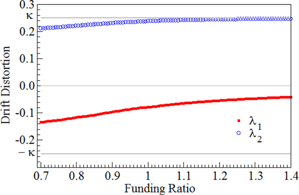
The decision of nature is displayed in Figure 2. We showed λ 1 and λ 2 as a function of the present funding ratio C 0. To facilitate the comparison, we put the two perturbations in one graph. We found that λ 1 is negative at any funding ratio level but is close to zero when C 0 is high; λ 2 is always positive and converges to κ. We also found that the optimal choice of λ 1 and λ 2 is always on the circle  $\lambda _1^2 + \lambda _2^2 = \kappa ^2$, which means the worst-case scenario is always at the boundary of the uncertainty set.

Figure 2. Static optimal perturbations λ 1 and λ 2. This figure depicts the optimal λ 1 and λ 2 as functions of the present funding ratio C 0 under the benchmark scenario with μ = 0.04, σ = 0.16, r = 0, a = 0, b = 0.1, ρ = 0.5, κ = 0.25, and T = 5. Nature makes decisions of λ 1 and λ 2 at time 0 under the constraint  $\lambda _1^2 + \lambda _2^2 \le \kappa ^2$ so as to maximize the expected shortfall at period T.
Figure 2 shows that a negative λ 1 and a positive λ 2 lead to the worst-case scenario. This is because the agent is afraid that the true expected asset return is lower than the estimated value, and the true liability return is higher than the estimated result. The resulting negative λ 1 represents the fear of an overestimated asset return. Hence, the absolute value of λ 1 is increasing with the exposure to the stock market, w. We know from Figure 1 that risk exposure and the funding ratio are negatively related. The lower the funding ratio, the higher the risk exposure will be and therefore the more negative the value of λ 1 will be. In contrast, if the funding ratio is sufficiently high, both the λ 1 penalty as well as the weight in the risky asset are smaller. The penalty term λ 1 also plays a role in the liability return. A negative λ 1 can benefit the agent by reducing the expected liability return. To capitalize on the fear of an increase in the liability return, nature chooses a positive λ 2 so as to compensate for the negative effect from λ 1 and to increase the liability growth, making the liability more costly.
We further examined how the perturbation terms impact the expected returns. Figure 3 displays both the naive and robust mean rates of the stock return and the liability return as functions of C 0. Without the preference for robustness, both drift terms are constant. However, if the investor is aware of the model misspecification, the perturbed expected stock return is dragged down by |σλ 1| due to the negative impact of λ 1. Despite the mixed sign of λ 1 and λ 2, the worst-case liability drift is pushed up by  $\vert b\rho \lambda _1 + b\sqrt {1 - \rho ^2} \lambda _2\vert$ since the positive effect of λ 2 dominates the drift distortion. In general, the robust policy differs from the naive one in the sense that the robust agent requires an additional guarantee on top of the naive contract in order to neutralize the estimation error. In other words, the robust policy needs more capital to hedge downside risks.

Figure 3. Mean rate of stock and liability return with and without the preference for robustness. This figure displays the expected stock and liability returns before and after considering parameter uncertainty as functions of the present funding ratio. Panel 3a comparing the robust stock drift μ S = μ + σλ 1 with the naive drift term μ S = μ. Panel 3b comparing the robust liability drift term  $\mu _L = a + b\rho \lambda _1 + b\sqrt {1 - \rho ^2} \lambda _2$ with the naive one μ L = a under the benchmark scenario.
3.3 Policy evaluation
The robust policy is less sensitive to the parameter misspecification. In this section, we will show how and when the agent can benefit from the robust policy. Let Q(w, δ) be the cost of hedging following a particular policy w, where δ is the assumed value of the drift parameters. In our case, the cost of hedging is defined by
 $$Q\left( {w,\delta} \right) = {\rm {\opf E}}\left[ {{\left( {L_T - A_T} \right)}^ + \vert w,\delta} \right].$$
The optimal hedging policy has a cost  $q(\delta ) = \mathop {\min} \limits_w Q\left( {w,\delta} \right)$ for given δ. Let δ 0 be the true value of δ, and denote q(δ 0) as the minimum hedging cost when the investor implements the associated optimal hedging policy w 0 under the true value δ 0. Any other alternative hedging policies
  $w_a (w_a \ne w_0)$ have higher expected shortfall.
Define the loss function K(w a|δ 0) as the difference between the cost of hedging following a suboptimal policy w a and the true minimum cost. The ‘cost of hedging’ here is defined as the initial wealth required to obtain a particular level of expected shortfall, denoted Q(w a, δ 0), which gives the loss function
 $$K\left( {w_a \vert \delta _0} \right) = Q\left( {w_a,\delta _0} \right) - q(\delta _0).$$
If δ ≠ δ 0, the agent is facing estimation error, therefore w a ≠ w 0 and K(w a|δ 0) > 0.
The agent does not know the true value of the drift terms δ 0. Given the estimated drift terms δ, she can choose between two alternative hedging policies, a robust policy w rob and a naive policy w na. At the benchmark scenario when the present funding ratio  $C_0 = 80\% $, the solutions are w rob = 0.81 and w na = 0.87. When
  $C_0 = 90\% $, we found that w rob = 0.67 and w na = 0.69. The robust policy will perform better than the naive policy, if
 $$K\left( {w_{rob} \vert \delta _0} \right) \lt K\left( {w_{na} \vert \delta _0} \right).$$
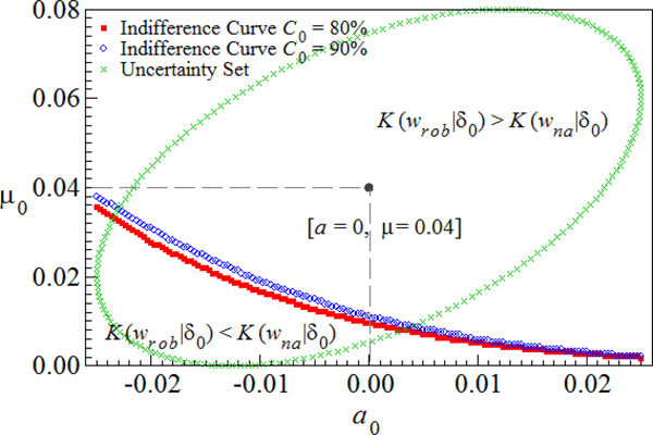
We displayed the loss indifference curves in Figure 4 when the present funding ratio is 80% and 90%. The x-axis and y-axis represent the true value of liability return a 0 and asset return μ 0, respectively. The point [a = 0, μ = 0.04] represents the estimated expected return δ. We also displayed the ellipsoid uncertainty set of the true drift term δ 0 in the figure.

Figure 4. Loss function equivalent curves. The figure plots the indifference curve of the loss when K(w rob|δ 0) = K(w na|δ 0). y-axis is the true value of the expected stock return μ 0 and x-axis is the true value of the liability drift a 0. The estimated value is μ = 0.04 and a = 0. The solid-dot indifference curve represents the case when  $C_0 = 80\% $ and the open-dot curve is the when
  $C_0 = 90\% $. In the region below the curve, the robust policy outperforms the naive policy, and in the region above, it is the other way around.
When K(w rob|δ 0) = K(w na|δ 0), the two policies require the same amount of wealth to hedge. In the region below the curve for both scenarios (when  $C_0 = 80\% $ and
  $90\% $), the robust policy requires less initial wealth than the naive policy to hedge a certain amount of expected shortfall. We call this area the robust policy's ‘beneficial region’. Hence, we can conclude that when the true drift term δ 0 is overestimated, the robust policy performs better.
This beneficial region is positively related to the present funding ratio C 0. Since the additional cost of hedging by following a robust policy increases as C 0 decreases, a lower C 0 leads to a smaller beneficial region. When liabilities are covered, the difference between a robust and a naive policy is subtle and the robust investor's beneficial region should also be larger.
3.4 Sensitivity analysis
The correlation parameter ρ, representing the completeness of the market, plays an important role in the model. If ρ = ±1, and λ 1 = λ 2 = 0, then the market becomes complete and the unhedgeable risk driver W 2 does not play a role. In this section, we investigated how sensitive the optimal hedges are with respect to a change of ρ.
In Figure 5, we show an extreme case when ρ = 1. The non-traded risk driver W 2 disappears from the liability diffusion process, and the perturbation parameter λ 2 does not play a role either. Nature can only control λ 1 to maximize the expected shortfall at period T. The naive agent considers this as a complete market. However, the robust agent still faces another source of incompleteness, caused by model misspecification.

Figure 5. Sensitivity analysis with ρ = 1. The figure depicts the optimal portfolio choice when ρ = 1. The remaining parameters stay at the benchmark level. The solid-dot line represents the robust policy and the empty-dotted curve is the naive policy. The naive agent considers such an economy a complete market, since the non-tradable risk driver W 2 is gone. However, the robust agent still stays in the incomplete market, because the model misspecification ( $\lambda _1 \ne 0\; \lambda _2 \ne 0$) is also considered as another source of market incompleteness.
With a low funding ratio, the robust policy deviates from the naive one much more severely compared with the benchmark case. When the asset risk and the liability risk are perfectly correlated, nature will choose a more negative λ 1 so as to maximize the expected shortfall. Although a negative λ 1 reduces the expected liability return as well, the liability drift term is less sensitive to the change of λ 1 than the expected asset return, since σ > b. As a result, the robust investor's fear of an overestimated asset return is stronger than the benchmark level.
In the case of overfunding, the two policies are identical. The hedging error volatility becomes  $\sigma _C^2 = \left( {w\sigma - b\rho} \right)^2$. The investor can fully replicate the liability by following a δ-neutral strategy
  $w = ((b\rho )/\sigma ) = 62\% $ if she has sufficient assets. In that case, robustness does not play a role because the δ hedge neutralizes the λ 1 effect.
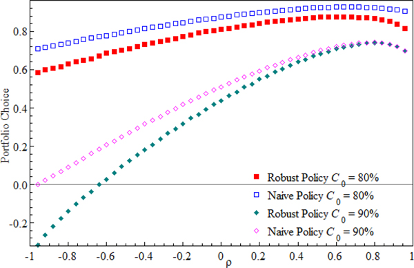
In Figure 6, we show the two hedging policies as a function of correlation parameter ρ. We displayed two scenarios, one when  $C_0 = 80\% $ and the other when
  $C_0 = 90\% $. The relation between the optimal portfolios and ρ is not monotone but is hump shaped. This is because the volatility of the value function σ C is a quadratic function of ρ.

Figure 6. Sensitivity analysis with respect to ρ. The figure plots the optimal naive and robust hedging policies as a function of correlation parameter ρ. We show two pairs of comparison: one with the present funding ratio C 0 of 80%, and the other with  $C_0 = 90\% $. The solid-dot curves represent the robust policy and the empty-dot curves are the naive policy.
The optimal portfolio initially increases with ρ for both policies because the liability is more exposed to the tradable risk driver W 1. Therefore, the risky portfolio has to increase as well, in order to hedge the traded liability risk. The optimal portfolio reaches the peak where ρ maximizes the total volatility σ C. After the peak, the risky portfolio goes down with ρ, because after the peak, any higher level of correlation will reduce σ C. From Figure 6, we can also see that the difference between the two policies under the lower funding ratio is wider than under the higher C 0.
4 Dynamic robust optimization
In this section, we will extend the problem to a dynamic strategy. The robust investor still aims to minimize the final-period expected shortfall under the worst-case scenario, but instead of making a static portfolio choice, she is now considering a dynamic optimal portfolio. Nature also can rebalance her choice of (λ 1t, λ 2t) instantaneously given the intertemporal decision of w t. We employed dynamic programming to solve this robust optimization problem.
4.1 Dynamic programming
Define the indirect utility function V(A t, L t), which follows the min–max expected utility given by (9). Both the investor and nature have a planing horizon of T. We omited the time subscript t for notation convenience. Using Feynman–Kaç, we can derive the Hamilton–Jacobi–Bellman equation (henceforth HJB) or partial differential equation (pde) for the investor's min–max problem:
 $$\eqalign{0 = & \mathop {\min} \limits_w \mathop {\max} \limits_{\lambda _1,\lambda _2} V_t + V_AA\left( {r + w(\mu - r) + w\sigma \lambda _1} \right) + V_LL\left( {a + b\rho \lambda _1 + b\sqrt {1 - \rho ^2} \lambda _2} \right) \cr & + \displaystyle{1 \over 2}V_{AA}w^2\sigma ^2A^2 + \displaystyle{1 \over 2}V_{LL}b^2L^2 + V_{AL}b\rho w\sigma AL - \displaystyle{1 \over 2}\nu \left( {\lambda _1^2 + \lambda _2^2 - \kappa ^2} \right),} $$
where the partial derivative with respect to x is denoted as V x. We formed a Lagrangian function with multiplier ν over the boundary condition:  $\lambda _1^2 + \lambda _2^2 \le \kappa ^2$.Footnote 4
By solving a linear system of equations based on the first-order condition of (16) with respect to the strategy variables w, λ 1, and λ 2, we have
 $$w^{^\ast} = - \displaystyle{{\left( {\mu - r} \right)V_AA\nu} \over {\sigma ^2\left( {V_{AA}A^2\nu + V_A^2 A^2} \right)}} - \displaystyle{{V_{AL}ALb\rho \sigma \nu + V_LV_AALb\rho \sigma} \over {\sigma ^2\left( {V_{AA}A^2\nu + U_A^2 A^2} \right)}},$$
 $$\lambda _1^{^\ast} = - \displaystyle{{\left( {\mu - r} \right)V_A^2 A^2\sigma} \over {\sigma ^2\left( {V_{AA}A^2\nu + V_A^2 A^2} \right)}} - \displaystyle{{b\rho \left( {V_{AL}ALV_AA - V_LLV_{AA}A^2} \right)} \over {\left( {V_{AA}A^2\nu + V_A^2 A^2} \right)}},$$
 $$\lambda _2^{^\ast} = \displaystyle{{V_LLb\sqrt {1 - \rho ^2}} \over \nu}.$$
This is a partial solution. The Lagrange multiplier ν, as well as V A, V AA, still need to be solved numerically.
The sign of the optimal λ 2 must be positive since it increases the expected liability return but does not influence the pension asset. The sign of λ 1 is ambiguous. A positive λ 1 not only increases the liability but also the asset, but the net effect depends on the value of other input variables.
The solution (17) has an interesting structure. The dynamic optimal investment strategy w* is a trade-off between hedging and speculation. We can see this by considering the extreme case when  $\nu \to 0$ and ν → ∞.
For ν → 0, the discrepancy parameters λ 1 and λ 2 have more freedom to choose an arbitrarily large aversion pair of drift for the Brownian motions, or in other words, the agent is extremely pessimistic about the approximation model. When ν → 0, we have
 $$w_{\nu \to 0}^{^\ast} = - \displaystyle{{V_LL} \over {V_AA}}\displaystyle{{b\rho} \over \sigma}. $$
This is a pure hedging portfolio, where the agent invests an amount in risky assets such that the change in the value function due to L is (as much as possible) offset by a change in value due to a. It is not possible to completely eliminate the volatility of L. This is because the liabilities are exposed both to hedgeable risk W 1 and unhedgeable risk W 2, but only the hedgeable part W 1 can be eliminated.
The optimal value for  $\lambda _1^* $ when ν → 0 is given by
 $$\lambda _{1,\nu \to 0}^{^\ast} = - \displaystyle{{\mu - r} \over \sigma} - \displaystyle{{b\rho \left( {V_{AL}V_A - V_LV_{AA}} \right)L} \over {V_A^2}}, $$
which contains two terms. The first term is the observable market price of risk, which we can see from the BS setup. The second term is more interesting. Since
 $$- \displaystyle{{b\rho \left( {V_{AL}V_A - V_LV_{AA}} \right)L} \over {V_A^2}} = \sigma \displaystyle{{\partial (w_{\nu \to 0}^{^\ast} A)} \over {\partial A}} = w_{\nu \to 0}^{^\ast} \sigma + \sigma A\displaystyle{{\partial w_{\nu \to 0}^{^\ast}} \over {\partial A}},$$
this reflects to what extent the agent's best possible hedging strategy is influenced by the instantaneous wealth level A t.
At the other extreme, when ν → ∞, both λ 1 and λ 2 shrink to zero, so κ = 0. This corresponds to the case when the agent faces no model misspecification. Hence, we recovered the ‘classical’ Merton's solution for the optimal portfolio choice:
 $$w_{\nu \to \infty} ^{^\ast} = - \displaystyle{{\mu - r} \over {\sigma ^2}}\displaystyle{{V_A} \over {V_{AA}A}} - \displaystyle{{V_{AL}L} \over {V_{AA}A}}\displaystyle{{b\rho} \over \sigma}. $$
The first term is a speculative portfolio, where the agent invests in the stock market to obtain the optimal trade-off between the observable market price of risk ((μ − r)/σ 2) and the local risk aversion − ((V A/V AAA)). The second term is the intertemporal hedging component, but the optimal amount to hedge is now measured in terms of the ‘CAPM-β’. That is, the optimal hedge is the local covariance term bρσ divided by local variance term σ 2, i.e. the stock market investment that minimizes locally the (unhedgeable) variance in the portfolio.
4.2 Numerical solution
As we cannot solve the PDE analytically, we will present numerical results for the dynamic optimization problem.
In Figure 7, we show the dynamic robust investment policy as a function of the instantaneous funding ratio C t and hedging horizon T. The optimal weight on the risky asset depends both on the solvency condition and the investment horizon. If the funding ratio is low, a longer term investor takes less risk than a shorter term investor. In other words, the risk exposure to the stock market decreases with the hedging horizon. When underfunded, an investor would take an aggressive risk position, betting on the chance of avoiding a shortfall, exactly as we have seen in the static case. A shorter planning horizon triggers a stronger intention to cover the liabilities, hence leads to a riskier position. However, when overfunded (C t > 1), the longer the investment horizon is, the more risk can be taken. The optimal portfolio converges to the hedging ratio δ ((bρ)/σ) when the hedging horizon T is close to zero.

Figure 7. Dynamic robust optimal hedging strategy. This figure displays the robust optimal investment policy as a function of the instantaneous funding ratio C t with benchmark input parameters under different hedging horizons. Panel 7a plots the robust portfolio choice as a function of the instantaneous funding ratio and the investment horizon T. Panel 7b depicts the solutions when investment horizon is T = 1, 3, 5. Due to technical limitations, our grid searching interval for the risky portfolio w has to be smaller than 1.95, otherwise we will confront a negative probability problem in some trinomial trees.
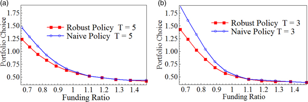
Next, we investigated the difference between the robust and the naive dynamic policies. In Figure 8, we present the two investment policies as a function of the instantaneous funding ratio under two hedging horizons, T = 5 and T = 3. We highlight two findings from the figure. First, the robust policy is less risky than the naive one as long as the instantaneous funding ratio is lower than 1. Second, the difference between the two policies decreases with the investment horizon. As the risk exposure decreases with hedging horizon, so does the fear of uncertainty. Compared with static hedges (Figure 1), dynamic hedges (Figure 8) take riskier positions under both robust and naive policies.

Figure 8. Dynamic robust and naive optimal hedging strategy as a function of instantaneous funding ratio at selected hedging horizon. In this figure, we display both robust and naive investment policies as functions of the instantaneous funding ratio. Panel 8a plots the solution when T = 5. Panel 8b shows the result when T = 3.
Figure 9 shows the dynamic optimal λ 1, λ 2 as functions of the funding ratio at three different investment horizons. It is still the case that λ 1 is always negative and λ 2 is always positive (see also Figure 2). We now focus on the dynamic effect of the processes.

Figure 9. Dynamic optimal perturbation processes. In this figure, we show the optimal perturbation processes λ 1 and λ 2 as functions of the instantaneous funding ratio when hedging horizon equals to T = 1, 3, 5. The solid lines are the movement of λ 1 and λ 2 when T = 5, the dashed curves are for the case T = 3, and the dotted curves are for T = 1. The upper panel with positive perturbations gives the optimal results of λ 2. The negative portion of the figure gives the optimal solutions of λ 1.
When underfunded (C t < 1), the absolute value of λ 1 decreases when the hedging horizon increases, since the longer term investor is less exposed to the stock market (see Figure 7b) than the shorter term investor. Therefore, nature becomes less effective in distorting the asset model when the hedging horizon increases. The optimal value of λ 2 increases with the investment horizon so as to offset the diminished effect of λ 1.
We moveed on to analyze the dynamic perturbed drift terms displayed in Figure 10. Panel 10a plots the perturbed expected stock return process μ S as a function of C t under three different investment horizons. Since μ S = μ + σλ 1 is a linear function of λ 1, it shares common characteristics with λ 1 shown in Figure 9. After all, μ S increases with hedging horizon when underfunded and vice versa if C t > 1. Panel 10b shows the movement of μ L. When C t is low, the perturbed expected liability return μ L increases with T to offset the diminishing distortions from the asset side.

Figure 10. Dynamic perturbation effect on drift terms. In this figure, we plot the dynamic movement of the perturbed drift terms as functions of the instantaneous funding ratio when hedging horizon is T = 1, 3, 5. Panel 10a depicts the movement of μ S = μ + σλ 1 and panel 10b shows  $\mu _L = a + b\rho \lambda _1 + b\sqrt {1 - \rho ^2} \lambda _2$.
4.3 Dynamic policy evaluation
From the static case, we know that the robust policy performs better when the drift terms are overestimated. In this section, we will investigate the effect of the hedging horizon.
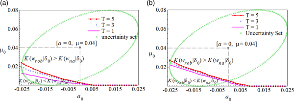
Figure 11 displays the policy indifference curve under different hedging horizons T. The area beneath the indifference curves represents the scenarios that require less initial wealth to hedge a given amount of downside risks by following a robust policy. Different from the static case (Figure 4), the beneficial region of the robust policy in the dynamic setting is smaller than it is in the static case. This means naive dynamic hedging is less sensitive to parameter uncertainty. Additionally, we found that the beneficial region increases with the hedging horizon. Therefore, long-term investors should be more inclined to follow a robust investment strategy than short-term investors. The horizon effect is weaker when the instantaneous funding ratio is relatively high. As a robustness check, we also conducted sensitivity analysis on ρ in the dynamic hedging environment when the instantaneous funding ratio is low. The hedging portfolios for both policies are positively related to the correlation factor ρ and are lower under longer term investment.
Figure 11. Dynamic loss function equivalent curve. The figure shows the policy indifference curve at a function of the true drift terms (μ 0, a 0) at three different horizons T = 1, 3, 5. The left panels plots the case when the instantaneous funding ratio equals to  $80\% $, and the right panel is the case when
  $C_t = 90\% $. The robust policy are better off in the area beneath the indifference curves. The dynamic policies w rob and w na are determined based on the estimated drift terms with values μ = 0.04 and a = 0.
5 Conclusion
We analyzed a robust hedging strategy under the condition that the market is incomplete and the underlying model can be misspecified. We employed and simplified the general model uncertainty problem of Hansen and Sargent (Reference Hansen and Sargent2007) to uncertainty about the drift terms. The robust policy requires an extra cost of capital, or lower liability discount rate, to guarantee against model uncertainty. That is the price to pay for coping with the parameter uncertainty. If the model is truly misspecified, the hedging will be more successful.
From our analysis, we summarize two major characteristics of the robust policy. We first found that the robustness effect strongly depends on the instantaneous funding ratio. The preference for robustness only influences the hedging policy when the funding ratio is low; if the fund's assets are large enough to cover the liability payoff, then the robust and the naive policies are identical. Second, the robust policy also becomes more valuable for longer investment horizons.
The investor can benefit from the robust policy when the expected return is overestimated. That means, with a given expected-shortfall hedging target, the robust policy requires less initial wealth to obtain a successful hedge than the naive policy if the true expected stock return is lower than the estimated value.
Acknowledgements
The authors thank two anonymous referees and the editor Clemens Sialm for extremely valuable suggestions and comments. The authors are also grateful for comments from Jaap Bos, Alexey Rubtsov, Bertrand Melenberg, Marcel Rindisbacher, Hans Schumacher and Michel Vellekoop. This research is financially supported by Netspar. All errors are our own.