


1. Introduction
The flow of inertial–buoyancy gravity current is well described by a horizontal thin-layer smooth propagation. However, when this flow encounters a vertical barrier (wall) a drastic change of pattern occurs. The arrested fluid becomes significantly thicker and a backward propagation, typified by a steep front, develops. This ‘reflection’ is of both practical and academic interest. The gravity current is governed by the thin-layer approximation termed shallow-water equations. The variables are the thickness (height)  $h(x,t)$ and the velocity
  $u(x,t)$ of the flow, where
  $x$ and
  $t$ are the horizontal coordinate and the time. The equations express volume and momentum balance, and form a system of two partial differential equations of hyperbolic type. The solution of such systems admits discontinuities, and hence the reflected front is conveniently treated as a reflected jump, bore or shock.
The classical prototype problem is concerned with the gravity current of a dense fluid in a non-restricting low-density ambient (such as water in air) generated by the dambreak (at position  $x=0$ and time
  $t=0$) of a long horizontal reservoir of depth
  $H$, and the reflection from a vertical smooth wall at
  $x = 2 L$. It is convenient to scale the height variable
  $h$ with
  $H$, the velocity
  $u$ with
  $(g H)^{1/2}$, the horizontal length with
  $L$ and the time with
  $L/(g H)^{1/2}$, where
  $g$ is the gravity acceleration. The scaled position of the obstacle (wall) is
  $x=2$. See figure 1. We assume that
  $H/L \ll 1$, the influence of the sidewalls is negligible, and the backwall of the reservoir is far away from the dam (consistent with the major analysis of Hogg & Skevington Reference Hogg and Skevington2021) and hence the only obstruction and reflection is from the wall at
  $x=2$. We emphasize the choice of the horizontal scale
  $L$: half the distance between the dam and the obstacle (wall). Viscous and surface tension effects are neglected.

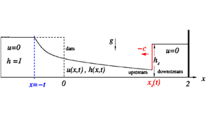
Figure 1. Sketch of the dambreak at  $x=0, t=0$, reflected from the wall at
  $x=2, t = 1$, as a jump of velocity
  $c$. Here
  $+,-$ denote upstream/downstream conditions at
  $x_s$. In our model the fluid downstream of the jump is (almost) stagnant with a horizontal top interface.
The mathematical advantage of this set-up is that the governing shallow-water equations are amenable to solution by the reliable method of characteristics. Such theoretical investigations were carried out by Greenspan & Young (Reference Greenspan and Young1978) and recently revisited and extended by Hogg & Skevington (Reference Hogg and Skevington2021), referred below as Reference Hogg and SkevingtonHS. However, in presence of reflected jumps, the solution by characteristics is an applied-mathematical challenge. Progress requires significant sophistication, such as series expansions (that restrict the time of relevance) and implementation of the hodograph transformation. The latter results are accurate for long times, but difficult for interpretation and extensions by researchers and engineers not familiar with the mathematical tools used for the solution.
This paper reports a simplified approach to the problem. The underlying idea is that the fluid left behind (downstream) the jump is (almost) stagnant, or, to be more precise, the speed  $u$ in
  $(x_s, 2]$ is much smaller than that of the jump,
  $c$; see figure 1. The justifications are as follows. (1) The fluid particles impinging on the wall are expected to convert the kinetic energy into height and pressure, forming a stagnant domain. However, the left vertical boundary, i.e. the jump, of this stagnant fluid must move with a significant speed to accommodate the increasing volume of the arrested fluid. (2) The solutions reported by Reference Hogg and SkevingtonHS strongly support this expectation. For the classical dry-bottom case, figure 5(b) of Reference Hogg and SkevingtonHS displays a very small
  $u$ in the domain between the jump and the wall. For the tailwaters case, Reference Hogg and SkevingtonHS report a ‘first stage’ with
  $u=0$ in the relevant domain (as discussed later in § 3). (3) This stagnant-downstream assumption in the analysis of reflected bores from the wall of a reservoir in two-layer gravity currents has been corroborated by experiments and simulation (see Baker, Ungarish & Flynn Reference Baker, Ungarish and Flynn2020; Ungarish Reference Ungarish2020); since there are physical similarities between the systems, we expect the same good performances in the present problem. We show that the use of this simplification in the problems analysed by Reference Hogg and SkevingtonHS renders a concise and insightful mathematical model. By some straightforward calculations, this model provides the speed, height and trajectory of the reflected jump as functions of time, and other useful estimates. Detailed comparisons with the more accurate predictions of Reference Hogg and SkevingtonHS show good agreement over long periods of propagation. We think that this is a useful model for both research and applications. Practically, the model changes the status of the problem from a matching-of-characteristics challenge to a straightforward calculation.
The structure of the paper: the simple model is derived in § 2; results for a dry bottom are shown and compared with Reference Hogg and SkevingtonHS. The extension to tailwaters systems is presented in § 3. Some concluding remarks are given in § 4. Appendix A summarizes the calculation of the horizontal flow prior to reflection for tailwaters and gravity currents.
2. Simple model formulation
Consider the motion of the reflected jump, see figure 1. The classical unbounded dambreak solution is
 \begin{equation} h(x,t) = ({4}/{9}) [ 1 - x/(2t) ] ^2, \quad u(x,t) = ({2}/{3}) (1 + x/t), \quad (x >{-} t). \end{equation}
We assume that the reservoir behind the dam is sufficiently long, so that the point  ${x = -t}, {h=1}$ of (2.1a,b) is not invalidated by the backwall for the time
  $t$ under consideration. The tip
  $h=0$ of the dambreak flow (2.1a,b) propagates with velocity
  $V=2$ and hits the wall at time
  $t_R = 1$, at which reflection (represented by the jump
  $x_s(t)$) starts. We note that the parabolic profile (2.1a,b) is valid also for the period
  $0< t< t_R$ in the domain
  $x < 2 t$.
We use a co-moving enclosing control volume about  $x_s(t)$. The flow variables in the upstream and downstream side are denoted by
  $+$ and
  $-$, respectively. The velocity of the jump is
  $c$. The volume and momentum (inertia supported by hydrostatic pressure forces) control-volume balances, or Rankine–Hugoniot conditions, are (see Reference Hogg and SkevingtonHS and Ungarish (Reference Ungarish2020) § 4.4)
 $$\begin{gather} {}[ (u-c) h ]^{+} = [(u-c) h ]^{-} , \end{gather}$$
 $$\begin{gather}{}[(u-c)^2~h]_-^+{=} - (1/2) [ h^2] _-^+ . \end{gather}$$
We also recall the kinematic equation
 \begin{equation} \frac{{\rm d} x_s}{{\rm d} t} = c, \end{equation}
with the initial condition  $x_s = 2$ at
  $t= t_R = 1$.
Evidently, (2.1a,b) gives explicitly  $h^+ = h(x_s,t)$ and
  $u^+=u(x_s,t)$. We denote by
  $h_s$ the height
  $h^-$. For a given pair,
  $t, x_s$, we have the two equations (2.2) for the three unknowns
  $c, h_s$ and
  $u^-$. To gain the additional information, Reference Hogg and SkevingtonHS performed a careful integration of the information carried on the reflected characteristics.
We argue that a significant simplification of the problem can be achieved by the following approximation (justified in § 1): the fluid in the downstream domain is arrested by the wall, and hence we set  $u^-=0$. Let
 \begin{equation} a = a(x_s,t) = \frac{h(x_s,t)}{h_s(t)}, \end{equation}
which is the height ratio of the fluid just before (upstream) and behind (downstream) the jump, expected to be smaller than  $1$ (otherwise, the dissipation is negative). Continuity (2.2a) gives
 \begin{equation} c ={-} [a /(1-a)] u(x_s,t). \end{equation}
We substitute this  $c$ into the momentum balance (2.2b), and after some algebra obtain
 \begin{equation} \frac{a}{ (1-a) (1+a)^{1/2} } = \frac{ \sqrt{h(x_s,t) }}{\sqrt{2} u(x_s,t)} = \frac{1}{\sqrt{2}} \frac{1 - x_s/(2 t)}{1 + x_s/t}, \end{equation}
where the last term comes from (2.1a,b). For given  $x_s$ and
  $t$ we can calculate
  $a$ and
  $c$ by (2.6) and (2.5). We have simple equations for the speed and height of the jump. We can integrate (2.3) to predict the position
  $x_s(t)$.
2.1. The jump at  $x=0$
$x=0$

Before performing the integration of  ${\rm d} x_s/ {\rm d} t$ we note that the position
  $x_s =0$ (the locus of the dam) provides some insights. We recall that at
  $x=0$ the speed and height (until the arrival of the jump) are the constant
  $u(x=0)= 2/3$ and
  $h(x=0)=4/9$ (see (2.1a,b)).
First, we note that for  $x_s=0$ the right-hand side of (2.6) is equal to
  $1/\sqrt {2}$ and the solution provides
  $a = 0.461$. We then obtain from (2.4) and (2.5) for the jump at
  $x_s=0$
 \begin{equation} h_s = 0.964, \quad c ={-} 0.570. \end{equation}
Next, we estimate the time  $t_D$ at which the reflected jump arrives at the dam position. We use volume balances. The volume transported to the right (figure 1) during
  $t_D$ at
  $x=0^-$ is equal to the volume between the jump (at
  $x_s=0^+$) and the wall at
  $x=2$. Since the fluid behind the jump is stagnant, the height of the interface must be quasi-constant, i.e.
  $\approx h_s$. This is expressed as
 \begin{equation} u(x=0) \times h(x=0)\times t_D = ({8}/{27}) t_D = 2 h_s = 1.928, \end{equation}
providing  $t_D = 6.48$. This turns out to be a good estimate; the accurate integration, considered below, predicts
  $t_D= 5.99$. The reason for the discrepancy is the present assumption that
  $h=h_s$ in the arrested domain
  $[0,2]$. Actually, the average height is expected to be slightly smaller than at the jump, and hence the volume in this domain is slightly smaller than
  $2 h_s$ used in (2.8), and a reduction of
  $t_D$ is expected. The useful insight is that the time of return from the wall to the dam is approximately five times longer than the time of flow from the dam to the wall. The reflected flow at the dam attains (almost) the initial height
  $h=1$ of the reservoir, see (2.7a).
2.2. Reflected jump results
The assumption  $u^- =0$ renders the model
 \begin{equation} \frac{{\rm d} x_s}{{\rm d} t} ={-} \frac{2}{3} \frac{a}{1-a} (1 + x_s/t), \end{equation}
where  $a$ is given by the non-linear equation (2.6). The initial conditions are
  $x_s = 2^-$ at
  ${t = 1^+}$. The numerical calculation of
  $x_s(t)$ is straightforward, using a standard method for (2.9) (e.g. Runge–Kutta) while
  $a$ is obtained by an iterative solver (e.g. the secant method) for (2.6) at the necessary gridpoints. Practically, we start the integration at
  $t=1 + \epsilon, x_s = 2 - \epsilon$ where
  $\epsilon$ is small,
  $10^{-4}$ say; this gives a tiny initial push to the jump. As a by-product of this solution we also obtain the speed of the jump
  $c = {\rm d} x_s/{\rm d} t$ and the height
  $h_s = (4/9)[1 - x_s/(2t)]^2/ a$ at the time steps. The computational time is insignificant.
Model results of the propagation of the jump are shown in figure 2, and compared with the more accurate solution of Reference Hogg and SkevingtonHS. The agreement is very good. The values of  $h_s(t)$ and
  $-c(t)$ predicted by the model are given in figure 3(a).

Figure 2. Graph of  $x_s$ vs
  $t$. The solid lines show results of the present model: blue line for direct integration; red line for ‘long-time’ formula (2.14) starting at
  $t_1=8$. The dash-dot line shows the predictions of Reference Hogg and SkevingtonHS.

Figure 3. Model predictions (a)  $h_s$ and
  $-c$ as functions of
  $t$. (b) Height at wall, compared with Reference Hogg and SkevingtonHS figure 4(b) results
  $h(2,t)$.
The depth of the fluid layer at the wall,  $h_w$, for
  $t >1$ is also of interest. In our simplified model we assume that the interface behind (downstream) the jump is horizontal,
  $h = h_w(t)$. The first approximation is that this interface is at height
  $h_s(t)$. However,
  $h_s$ is determined by the local conditions at
  $x_s$, and hence a correction that takes into account the entire volume in the arrested domain is suggested. In a realistic system a small adjustment flow in the ‘arrested’ domain is expected, and we argue that this will redistribute the volume accumulated between the jump and the wall to an almost flat domain of height
  $h_w(t)$ not necessarily equal to the instantaneous
  $h_s(t)$. The volume in this domain is
  $(2-x_s) h_w$. This volume has been contributed to
  $x>x_s$ by the unperturbed dambreak flow,
  $\mathcal {V}(t)$. For
  $x_s >0$ the accumulation of fluid begins from
  $\mathcal {V}(t_i)=0$ at
  $t_i = x_s/2$ upon the arrival of the tip, then dambreak
  $u h$ influx according to (2.1a,b). For
  $x_s <0$ there is initial fluid in the lock
  $\mathcal {V}(t_i) = -x_s$, then dambreak
  $uh$ influx. We calculate
  $\mathcal {V}(t)$ using
 \begin{equation} \frac{8}{27} \int_{t_i} ^{t} \left[1 + \frac{x}{t'}\right]\left[ 1 - \frac{x}{2t'}\right]^2 \,{\rm d} t' \end{equation}
for the contribution of the flux see (2.1). After some algebra, the balance gives
 \begin{equation} \mathcal{V}(t) = \frac{(2t - x_s)^3}{27 t^2} = (2-x_s)h_w, \end{equation}
and hence
 \begin{equation} h_w = \frac{(2t - x_s)^3}{27 t^2 (2 - x_s) }, \quad (t >1). \end{equation}
The results are displayed in figure 3(b) and compared with the predictions of Reference Hogg and SkevingtonHS. The agreement is good.
2.3. Long-time further simplification
Another useful simplification is for long time, when the reflected jump is already in the reservoir, i.e.  $x_s<0$. We note that in this stage of motion, the value of
  $h_s$ is close to 1. We have demonstrated that when the jump reaches
  $x=0$ at
  $t \approx 6$ then
  $h_s = 0.96$; figure 3(a) shows that the difference
  $1-h_s$ decreases with
  $t$. Consequently, it is justified to approximate
  $a(x_s,t) = h(x_s,t)/h_s$ by
  $h(x_s,t)$ for sufficiently large
  $t>t_1$ when
  $x_s<0$. (We take
  $t_1 =8$, see below.) This approximation slightly underestimates
  $a$ and
  $c$.
$c$.
The approximation  $a = h(x_s,t)$ and use of (2.1a,b) reduce the relationship (2.5) to
 \begin{equation} c = \frac{{\rm d} x_s}{{\rm d} t} ={-} \frac{u(x_s,t) h(x_s,t)}{1- h(x_s,t)} ={-} \frac{2}{3} \frac{(2 - \xi)^2 (1 + \xi)}{9 - (2 - \xi)^2}, \end{equation}
where  $\xi = x_s(t)/t$. The integration of (2.13) provides the implicit result
 \begin{equation} \frac{t}{t_1} = \frac{(8 - \xi_1)(1 + \xi_1)^2} {(8 - \xi )(1 + \xi )^2}, \end{equation}
where the initial condition  $\xi _1= x_s(t_1)/t_1$ is taken from the numerical integration of (2.9). The more explicit solution
  $x_s$ and
  $c$ as functions of
  $t$ (
$t$ ( $>t_1$) follows: we apply (2.14) for values of
  $\xi < \xi _1$ and obtain the corresponding
  $t$ (
$t$ ( $> t_1$); this provides
  $x_s(t) = \xi \times t$ (the limit is
  $\xi = -1$ for which
  $t \to \infty$). For each
  $x_s(t)$, the corresponding
  $c$ is given by (2.13).
We started the application of (2.14) with  $t_1=8,\ \xi _1 = -0.150$ and obtained the red line of figure 2. The numerical solution gives
  $h_s= 0.98$ at the starting
  $t_1 = 8$, and as time progresses the simplification
  $h_s = 1$ becomes more and more accurate. We thus estimate that the error of (2.14) is approximately
  $2\,\%$; we recall that the error is manifested as a reduction of
  $|c|$. The figure confirms that the approximation error is small. Surprisingly, the approximated curve in figure 2 is in better agreement with the Reference Hogg and SkevingtonHS results than the numerical integration of the model, but this must be considered a coincidence.
3. Reflection with tailwaters
In this system a layer of dense fluid of height  $h_0$ is present on the bottom before dambreak, see figure 7. Essentially, the process is as before: after dambreak at
  $t=0$ the fluid starts propagation from
  $x=0$ toward the wall at
  $x=2$. At time
  $t_R$ this propagation hits the wall and is reflected back. The reflection, see figure 4, is manifested by the jump
  $x_s(t)$ of height
  $h_s$ and velocity
  $c$. In the classical problem (
 $h_0 = 0$), the fluid approaching the wall has a sharp tip
  $h=0$ that moves with
  $V=u=2$. In the new problem, the fluid approaching the wall is a layer of height
  $h_f>h_0$ and velocity
  $u_f$ that forms behind a jump of velocity
  $V>u_f$. Note that
  $h_f,u_f$ and
  $V$ depend on
  $h_0$ and can be easily calculated from available shallow-water theory results (see Appendix A).

Figure 4. Dambreak at  $x=0$ with reflected jump from wall at
  $x=2$ with tailwaters. This is the first stage,
  $t_R< t< t_{SM}$. For
  $t>t_{SM}$ the horizontal domain disappears, like in figure 1.
The time  $t_R$ when the reflection starts for a given
  $h_0$ is given by
  $2/V$. Then, the flow upstream of the jump is composed of the domains: (1) a horizontal layer of constant thickness
  $h_f$ and constant velocity
  $u_f$ for
  $x>x_M(t)$; (2) the standard dambreak flow (2.1a,b) for
  $x \le x_M$. At
  $x=x_M(t)$ there is smooth transition (continuity) between the two domains. The values of
  $x_M(t), h_f, u_f$ can be easily calculated for a given
  $h_0$ (see Appendix A).
As for the  $h_0 =0$ case, the main objective is the calculation of the behaviour of the jump (
 $x_s, c, h_s$ as functions of
  $t$). This problem was solved by Reference Hogg and SkevingtonHS by characteristics in the hodograph plane. The more complex upstream domain when
  $h_0 >0$ complicates the solution. Again, a simplified model is expected to be beneficial.
Our model based on (2.3)–(2.6) can be applied to this problem with some straightforward modification. With the assumption that the fluid in the reflected domain  $x>x_s(t)$ is (almost) stagnant, the previous formulation remains valid for
  $h_0>0$. We only must (a) change the initial time to the correct
  $t_R$, (b) use the appropriate equations for the upstream
  $h,u$ encountered by the jump, i.e. reconsider the
  $\sqrt {h}/{u}$ term in (2.6); here we distinguish between two stages:
(1) In the first stage,
$t_R \le t \le t_{SM}$, the jump encounters constant upstream conditions $h_f,u_f$. The jump has constant $c$ and $h_s$ given by
(3.1a,b)with\begin{equation} c ={-} \frac{a u_f}{1-a}, \quad h_s =\frac{h_f}{a}, \end{equation}$a$ provided by
(3.2)At time\begin{equation} \frac{a}{ (1-a) (1+a)^{1/2} } = \frac{ \sqrt{h_f}}{\sqrt{2} u_f}. \end{equation}$t_{SM}$ the jump meets the point $M$ (which propagates from the dambreak time with velocity $u_f - \sqrt {h_f}$). The meeting position is $x_{SM}$, given by
(3.3)From these equations we obtain\begin{equation} x_{SM} = 2 + c (t_{SM}-t_R) = (u_f - \sqrt{h_f}) t_{SM}. \end{equation}$t_{SM}$ and $x_{SM}$. Note that for $h_0 >0.1383$ point $M$ moves into the reservoir (negative velocity).
It is interesting that for this stage the accurate solution of Reference Hogg and SkevingtonHS and the present model coincide. Indeed, (4.1) of Reference Hogg and SkevingtonHS express the same prediction as our (3.1a,b)–(3.2) for
$c,h_s$ in the first stage, using different notation. In other words, Reference Hogg and SkevingtonHS confirm the assumption of $u^- = 0$ for this stage. This gives additional support to the present model.(2) In the second stage,
$t>t_{SM}$, the jump encounters the classical parabolic-height dambreak domain (figure 1). We therefore apply the same formulation as in the $h_0=0$ case, i.e. we use (2.3)–(2.6). The difference with the $h_0=0$ case is that now the initial conditions for the integration of (2.3) are $x_s = x_{SM}$ at $t = t_{SM}$. We use exactly the same numerical solution as for the $h_0=0$ case. Moreover, we note that the long-time simplification result (2.14) is also relevant, with appropriate $t_1$ and $\xi _1$ conditions.


3.1. Reflected jump results for $h_0>0$

We calculated the solution for the example  $h_0 = 0.1318$ of Reference Hogg and SkevingtonHS, using the same formulas for the basic field before reflection, i.e. the same
  $h_f, u_f, t_R, t_{SM}, x_{SM}$ (in the Reference Hogg and SkevingtonHS paper, our points
  $M$ and
  $SM$ are called
  $P1$ and
  $P2$, respectively).
The shallow-water calculations (Appendix A) give  ${h_f = 0.4444}, {u_f =0.6667}, {t_R = 2.07}$. In the first stage by (3.1a,b) and (3.2), the jump has
  $c = 0,570, h_s = 0.964$. We obtain
  $t_{SM} = 5.58, x_{SM} = 0$. These are the boundary conditions for the calculations of the second stage (numerical integration). The model predictions for
  $h_0 = 0.1318$ are displayed in figure 5. The figure also shows the
  $x_s(t)$ results of Reference Hogg and SkevingtonHS. The agreement between the model and the accurate solution of Reference Hogg and SkevingtonHS is excellent. Actually, the agreement here is better than for
  $h_0 = 0$ in figure 2; this is not coincidence, as explained later in § 4.

Figure 5. Results for system with tailwaters  $h_0=0.1381$: (a)
  $x_s(t)$ red line for model, black dash-dot for Reference Hogg and SkevingtonHS, (b)
  $h_s$ and
  $-c$ vs
  $t$.
$t$.
To gain further insights, figure 6 shows model predictions for  $x_s, h_s$ and
  $c$ as functions of
  $t$ for various
  $h_0$. We conclude that the presence of the tailwaters layer
  $h_0>0$ contributes three major effects (compared with the
  $h_0 = 0$ case): the start of the reflection is delayed, the initial stage of reflection is with constant
  $h_s$ and
  $c$, and the speed of propagation of the jump is larger. These effects are clearly pointed out by the present simplified model, in full agreement with the more accurate solution of Reference Hogg and SkevingtonHS. The interpretation of these effects is as follows. The front
  $V$ from the dam to the wall is delayed by the task of setting in motion the stagnant layer of thickness
  $h_0$, hence the increase of time
  $t_R$ when it reaches the wall. Typically,
  $t_R \approx 2$ (in contrast to 1 for
  $h_0 = 0$). The reflection jump encounters for a while a layer of constant
  $h_f, u_f$, therefore the jump conditions produce constant
  $h_s,c$. The layer impinging on the wall has from the beginning of the reflection a significant
  $h_f > h_0$. Consequently, the reflected jump has from the beginning a significant
  $a = h_f/h_s$, accompanied by a significant
  $c$ (compare figures 5b and 3a).

Figure 6. Model predictions  $x_s, h_s$ and
  $-c$ vs
  $t$ for system with tailwaters
  $h_0 =0.05, 0.15, 0.30$. The dash-dot line is the
  $x_s(t)$ approximation (2.14) for
  $h_0=0.3$.
We note that for  $h_0 \ge 0.15$ the value of
  $h_s$ is close to 1 within 3 % from the beginning. Within this error, the propagation in the second stage is provided by the approximation (2.14). In other words, the reflection behaviour can be obtained from only algebraic formulas: using the known
  $h_f, u_f, t_R$ we calculate
  $h_s$ and
  $c$ for the first stage, then obtain
  $t_{SM}$ and
  $x_{SM}$ from (3.3). This point is identified with
  $t_1$ and
  $\xi _1 = x_{SM}/t_{SM}$ in (2.14). The values of
  $x_s$ and
  $c$ for
  $t>t_{SM}$ follow. Tests have confirmed the good accuracy of this approximation. For example, in figure 6 for
  $h_0=0.3$ the
  $x_s$ lines obtained by numerical integration and approximation (2.14) almost coincide.
3.2. Gravity current in deep ambient
The previous systems were of water-in-air type. Consider a reservoir of fluid of density  $\rho _c$ embedded in a large ambient fluid of a smaller density
  $\rho _a$. The one-layer approximation formulation neglects the motion in the ambient. In this framework, the shallow-water equations for the gravity current and the internal-jump correlations reduce to these used in the previous analysis upon change of
  $g$ to the reduced gravity
  $g' = (1-\rho _a/\rho _c) g$ (Ungarish Reference Ungarish2020).
The dambreak behaviour of the one-layer general gravity current is quite similar to that of the tailwaters system considered in § 3: the reflected jump encounters first a horizontal layer, figure 7(b), then the parabolic-height profile. The calculations of  $h_f,u_f$ and
  $t_R$ are different from those of the
  $h_0>0$ case, see Appendix A, because in the free-propagation stage the nose of the gravity current is governed by a Benjamin-type condition. The subsequent calculation of the reflected jump is the same. Again,
  $g$ is replaced by
  $g'$ in the scaling.

Figure 7. Sketch of dambreak at  $x=0$ prior to reflection
  $(t< t_R$) in presence of tailwaters (a) and for a gravity current of moderate
  $\rho _a/\rho _c$ (b). Reflection starts when the front of speed
  $V$ reaches the wall.
4. Concluding remarks
We revisited the problem of the reflected flow produced by dambreak of a Cartesian long reservoir over a dry bottom ( $h_0=0$) and with tailwaters (
 $h_0>0$). We developed a simplified model for
  $x_s, h_s$ and
  $c$ (position, height and velocity) of the jump as functions of time based on the major assumption that the fluid between the vertical obstacle (wall) and the reflected jump is stagnant (more precisely,
  $|u^-/c| \ll 1$). This allows the solution of the problem by a straightforward numerical integration of an initial-value ordinary differential equation, in contrast with the previously published analytical results that were obtained by the method of characteristics which requires complicated mathematical manipulations for the solution of the reflected domain. For long times, a simple analytical approximation is also available. The model points out clear-cut effects of the presence of the the tailwaters. Surprisingly, for the more complex system
  $h_0>0$, the model is more accurate than for
  $h_0=0$, because the first stage result is identical with the solution of Reference Hogg and SkevingtonHS by characteristics, and in the second stage there is a large
  $|c|$ from the beginning that reduces the error of the neglected
  $| u^-/c |$.
The model does not provide the details of the flow in the reflected domain (speed  $u(x,t)$ and height
  $h(x,t)$), only the approximation
  $u=0$ and the average
  $h = h_w(t)$.
We admit that the model lacks formal justification, such as by a systematic expansion of  $u^-$ in the reflected domain that proves that the leading term is zero. We argue that this deficiency is relaxed by the fact that comparisons with accurate solutions could be performed. Indeed, the model has been validated by comparisons with the more accurate results of the recent paper of Reference Hogg and SkevingtonHS (obtained by significantly more complex methods). In all the tested cases we found very good qualitative compatibility and good quantitative agreement, for long periods of time. These agreements provide reliable justification to the simplifications used in our model. We therefore think that this model can be recommended with confidence for use in various research and engineering problems where a fair approximation is sufficient for the application. In our opinion, this is a significant change of status of the reflection problem, from a difficult analytical challenge to a quite standard off-the-shelf solution.
Acknowledgements
The author thanks Professor A.J. Hogg for useful discussions and for providing data for comparisons.
Declaration of interest
The author reports no conflict of interest.
Appendix A. Calculation of $h_f,u_f$ and $t_R$


A.1. Tailwaters
The dambreak generates a forward-propagating jump of height  $h_f$ and velocity
  $V$ that propagates fluid from the reservoir and also activates the fluid in the
  $h_0$-thick layer below, see figure 7. The jump conditions (2.2) apply with
  $V$ instead of
  $c$. This also yields
 \begin{equation} u_f = (1 - h_0/h_f) V. \end{equation}
The domain activated by the jump is supported by characteristics from the dambreak initial situation. The matching yields
 \begin{equation} u_f = 2(1 - \sqrt{h_f}), \quad 2h_0 u_f^2 h_f = (h_0 + h_f) ( h_f - h_0)^2. \end{equation}
We solve for  $h_f$, then calculate
  $u_f$ and
  $V$. Reflection starts when
  $V$ (formed at
  $t=0, x=0$) reaches the wall
  $x=2$, i.e. at time
  $t_R = 2/V$.
The constant-height domain is matched to the curved-interface domain at  $x_M$ given by the leading characteristic in the dambreak fan about
  $x=0, t=0$. This gives
 \begin{equation} x_M(t) = (u_f - \sqrt{h_f}) t. \end{equation}
A.2. Gravity current
The new parameters are the density ratio  $(\rho _a/\rho _c)$ and the height ratio of ambient-to-lock
  $\tilde {H}$. See figure 7(b). The nose of the gravity current propagates according to a jump condition (see Ungarish Reference Ungarish2020) typically provided by Benjamin's formula:
 \begin{equation} V = u_f = \left[ \frac{\rho_c}{\rho_a} \frac{(2 - \alpha)(1 - \alpha)}{1+\alpha} h_f \right]^{1/2}, \quad \alpha = h_f/\tilde{H}. \end{equation}
Matching with the initial-conditions, characteristics yield again  $u_f = 2(1 - \sqrt {h_f})$. We solve for
  $h_f$, then obtain
  $u_f$ and
  $V$. Reflection starts when
  $V$ (formed at
  $t=0, x=0$) reaches the wall
  $x=2$, i.e. at time
  $t_R = 2/V$. Equation (A3) is valid.
Consider the limit  $\rho _c/\rho _a \to \infty$. Evidently,
  $g' =g$. We also obtain (see Ungarish Reference Ungarish2020)
  $u_f=V=2, h_f =0$,
  $t_R =1$. The classical problem is recovered.


