2.1. SCIF algorithm

Consider a pair of state estimates $\lcub \hat{\bf x}_{i}\comma \; {\bf P}_{i}\rcub $, where i={1, 2}, and $\hat{\bf x}_{i}$ and ${\bf P}_{i}$ represent the estimated state vector and the corresponding error covariance matrix, respectively. If the two estimates are independent from one another, the fused state and its corresponding error covariance can be derived from the general Kalman filter relations (Julier and Uhlmann, Reference Julier and Uhlmann1997):

(1)$$\eqalign{{\bf P} &= \left( {{\bf P}_1^{-1} + {\bf P}_2^{-1} } \right) ^{-1} \cr \hat{{\bf x}} &= {\bf P}\left( {{\bf P}_1^{-1} {\hat{{\bf x}}}_1 + {\bf P}_2^{-1} {\hat{{\bf x}}}_2} \right)}$$

When there is correlation between these two estimates, the fused results in Equation (1) would be inconsistent and would have optimistic measures of their quality (Carrillo-Arce et al., Reference Carrillo-Arce, Nerurkar, Gordillo and Roumeliotis2013). To deal with the correlation between two estimates, CIF can be used (Julier and Uhlmann, Reference Julier and Uhlmann1997). CIF uses a convex combination of the means and covariances of the two estimates, which theoretically yields a consistent estimate for any degree of correlation between two input estimates:

(2)$$\eqalign{{\bf P}^{-1} &= \omega {\bf P}_1^{-1} + \lpar 1-\omega \rpar {\bf P}_2^{-1} \cr \hat{{\bf x}} &= {\bf P}\left[ {\omega {\bf P}_1^{-1} {\hat{{\bf x}}}_1 + \lpar 1-\omega \rpar {\bf P}_2^{-1} {\hat{{\bf x}}}_2}\right] }$$

where ω∈[0, 1] is a scalar parameter, which can be optimised with respect to different criteria, such as minimising the trace or the determinant of ${{\bf P}}$.

Consider two PLs, PL_i and PL_j, in a network of N PLs with states at time instant k denoted as ${\bf x}_{k}^{i} $ and ${\bf x}_{k}^{j} $, and their corresponding covariance ${{\bf P}}_{k}^{i} $ and ${{\bf P}}_{k}^{j} $, respectively. The relative measurement between the two PLs can be expressed as (Carrillo-Arce et al., Reference Carrillo-Arce, Nerurkar, Gordillo and Roumeliotis2013):

(3)$${\bf z}_k^{i\comma j} = {\bf H}_k^{i\comma j} \left( {{\bf x}_k^i -{\bf x}_k^j } \right) + {\bf n}_k^{i\comma j}$$

where ${\bf z}_{k}^{i\comma j}$ denotes the measurement, ${\bf H}_{k}^{i\comma j} $ is an orthogonal matrix which enables the state of either PL to be expressed in terms of the other PL state and ${\bf n}_{k}^{i\comma j}$ is the zero-mean white Gaussian measurement noise with covariance ${\bf R}_{k}^{i\comma j} $. PL_i is assumed to be the one of interest and has the prediction state ${{\hat{\bf x}}}_{k\vert k-1}^{i} $ and corresponding covariance ${{\bf P}}_{k\vert {k-1}}^{i}$ derived using standard Kalman Filter (KF) methods such as the Extended Kalman Filter (EKF). When the relative measurement from PL_j is received by PL_i the information on state ${{\hat{\bf x}}}_{k\vert {k-1}}^{j} $ and covariance ${{\bf P}}_{k\vert {k-1}}^{j} $ of PL_j is also shared with PL_i. With the received relative information, PL_i can directly generate an estimate and corresponding covariance from the relative measurement:

(4)$$\left\{{\matrix{ {\hat{{\bf x}}_k^{i*} = \hat{{\bf x}}_{k\vert k-1}^j + {\left( {{\bf H}_k^{i\comma j} } \right) }^T{\bf z}_k^{i\comma j} } \hfill \cr {{\bf P}_k^{i*} = {\bf P}_{k\vert k-1}^j + {\bf H}_k^{i\comma j} {\bf R}_k^{i\comma j} {\left( {{\bf H}_k^{i\comma j} } \right) }^T} \hfill \cr } } \right.$$

At this instant two pairs of state and corresponding covariance of PL_i, one from the time update and one from the relative measurement update, are derived. The fusion of these two pairs of estimates can then be performed using Equation (2). However, the relative measurement cannot always be expressed as in Equation (3) with an orthogonal matrix ${\bf H}_{k}^{i\comma j} $, which is often in a nonlinear form. When ${\bf H}_{k}^{i\comma j} $ is in any other form it is not possible to directly calculate ${{\hat{\bf x}}}_{k}^{i\ast } $ in Equation (4). To use the relative measurement to update the propagated state and covariance, a transformation of the relative measurements needs to be implemented. ${\bf x}_{k\comma m}^{i} ={\bf H}_{k}^{i\comma j} {\bf x}_{k}^{i} +{\bf n}_{k}^{i\comma j} $ can be derived from Equation (3) using the transformation (Li and Nashashibi, Reference Li and Nashashibi2013):

(5)$${\bf x}_{k\comma m}^i = {\bf H}_k^{i\comma j} \hat{{\bf x}}_{k\vert k-1}^j + {\bf z}_k^{i\comma j}$$

The covariance corresponding to ${\bf x}_{k\comma m}^{i} $ is given by ${{\bf P}}_{k\comma m}^{i} ={\bf H}_{k}^{i\comma j} {{\bf P}}_{k\vert {k-1} }^{j} \lpar {{\bf H}_{k}^{i\comma j} } \rpar ^{T}+{\bf R}_{k}^{i\comma j} $. The fusion can be performed after the relative measurement update in KF methods as follows:

(6)$$\eqalign{{\bf K}_k^* &= {\bf P}_{k\vert k-1}^i \left( {{\bf H}_k^{i\comma j} } \right) ^T \left[ {{\bf H}_k^{i\comma j} {\bf P}_{k\vert k-1}^i {\left( {{\bf H}_k^{i\comma j} } \right) }^T + {\bf P}_{k\comma m}^i }\right] ^{-1} \cr \hat{{\bf x}}_{k\vert k }^{i\comma *} &= \hat{{\bf x}}_{k\vert k-1}^i + {\bf K}_k^* \left( {{\bf x}_{k\comma m}^i -{\bf H}_k^{i\comma j} \hat{{\bf x}}_{k\vert k-1}^i } \right) \cr {\bf P}_{k\vert k }^{i\comma *} &= \left( {{\bf I}-{\bf K}_k{\bf H}_k^{i\comma j} } \right) {\bf P}_{k\vert k-1}^i }$$

where ${{\hat{\bf x}}}_{k\vert k }^{i\comma \ast } $ and ${{\bf P}}_{k\vert k }^{i\comma \ast } $ are the updated state of the PL_i and its corresponding covariance without considering the correlation introduced by PL_j. Then, as in Equation (4), the propagated and updated states can be fused using Equation (2). This fusion can also be performed during the relative measurement update in a standard KF-based algorithm (Goel et al., Reference Goel, Kealy, Gikas, Retscher, Toth, Brzezinska and Lohani2017):

(7)$$\eqalign{{\bf K}_k &= {\bf P}_{k\vert k-1}^{i\comma sca} \left( {{\bf H}_k^{i\comma j} } \right) ^T \left[ {{\bf H}_k^{i\comma j} {\bf P}_{k\vert k-1}^{i\comma sca} {\left( {{\bf H}_k^{i\comma j} } \right) }^T + {\bf P}_{k\comma m}^{i\comma sca} } \right] ^{-1} \cr \hat{{\bf x}}_{k\vert k }^i &= \hat{{\bf x}}_{k\vert k-1}^i + {\bf K}_k \left( {{\bf x}_{k\comma m}^i -{\bf H}_k^{i\comma j} \hat{{\bf x}}_{k\vert k-1}^i } \right) \cr {\bf P}_{k\vert k }^i &= \left( {{\bf I}-{\bf K}_k{\bf H}_k^{i\comma j} } \right) {\bf P}_{k\vert k-1}^{i\comma sca} }$$

where ${{\bf P}}_{k\vert {k-1} }^{i\comma sca} ={{\bf P}}_{k\vert {k-1} }^{i} /\omega $ and ${{\bf P}}_{k\comma m}^{i\comma sca} ={{\bf P}}_{k\comma m}^{i} /\lpar {1-\omega } \rpar $ are two scaled covariances. Another way of performing the fusion during the relative measurement update is given by (Mokhtarzadeh and Gebre-Egziabher, Reference Mokhtarzadeh and Gebre-Egziabher2014):

(8)$$\eqalign{ {\bf P}_{k\vert k }^i &= \left[ {\omega {\left( {{\bf P}_{k\vert k-1}^i } \right) }^{-1} + \left( {1-\omega } \right) {\left( {{\bf H}_k^{i\comma j} } \right) }^T{\left( {{\bf P}_{k\comma m}^i } \right) }^{-1}{\bf H}_k^{i\comma j} } \right] ^{-1} \cr {\bf K}_k &= \left( {1-\omega } \right) {\bf P}_{k\vert k }^i \left( {{\bf H}_k^{i\comma j} } \right) ^T\left( {{\bf P}_{k\comma m}^i } \right) ^{-1} \cr \hat{{\bf x}}_{k\vert k }^i &= \hat{{\bf x}}_{k\vert k-1}^i + {\bf K}_k\left( {{\bf x}_{k\comma m}^i -{\bf H}_k^{i\comma j} \hat{{\bf x}}_{k\vert k-1}^i } \right) }$$

These two ways of accounting for the correlations have less computational cost than the one with fusion performed after the relative measurement update. Since the relative measurement used in this paper is in the form of inter-PL ranges, the correlated covariance components are limited to the states involved in the inter-PL ranges. To incorporate known independent information in the estimates based on the above described algorithms, they need to be modified using the following theory (Li and Nashashibi, Reference Li and Nashashibi2013):

(9)$$\eqalign{{\bf P}_1 &= {\bf P}_{1d}/\omega + {\bf P}_{1i} \cr {\bf P}_1 &= {\bf P}_{2d}/\lpar {1-\omega } \rpar + {\bf P}_{2i} \cr {\bf P}^{-1} &= {\bf P}_1^{-1} + {\bf P}_2^{-1} \cr \hat{{\bf x}} &= {\bf P} \left[ {{\bf P}_1^{-1} {\hat{{\bf x}}}_1 + {\bf P}_2^{-1} {\hat{{\bf x}}}_2} \right] }$$

where ${{\bf P}}_{1i}$ and ${{\bf P}}_{2i}$ are covariance components with known absolute independence and ${{\bf P}}_{1d}$ and ${{\bf P}}_{2d}$ are two correlated covariance components. Therefore, to use the SCIF algorithm, the scaled covariances in Equations (7) and (8) have to be added with the independent component before the measurement update. For example, Equation (7) can be changed to:

(10)$$\eqalign{{\bf K}_k &= {\bf P}_{k\vert k-1}^{i\comma all} \left( {{\bf H}_k^{i\comma j} } \right) ^T \left[ {{\bf H}_k^{i\comma j} {\bf P}_{k\vert k-1}^{i\comma all} {\left( {{\bf H}_k^{i\comma j} } \right) }^T + {\bf P}_{k\comma m}^{i\comma all} }\right] ^{-1} \cr \hat{{\bf x}}_{k\vert k }^i & = \hat{{\bf x}}_{k\vert k-1}^i + {\bf K}_k\left( {{\bf x}_{k\comma m}^i -{\bf H}_k^{i\comma j} \hat{{\bf x}}_{k\vert k-1}^i } \right) \cr {\bf P}_{k\vert k }^i &= \left( {{\bf I}-{\bf K}_k{\bf H}_k^{i\comma j} } \right) {\bf P}_{k\vert k-1}^{i\comma all} }$$

where ${{\bf P}}_{k\vert {k-1} }^{i\comma all} ={{\bf P}}_{k\vert {k-1} }^{i\comma sca} +{{\bf P}}_{k\vert {k-1} }^{i\comma {\rm id}} $ and ${{\bf P}}_{k\comma m}^{i\comma all} ={{\bf P}}_{k\comma m}^{i\comma sca} +{{\bf P}}_{k\comma m}^{i\comma {\rm id}} $ both consist of two covariance components ${{\bf P}}_{\cdot} ^{i\comma sca} $ and ${{\bf P}}_{\cdot}^{i\comma {\rm id}} $ representing correlated and independent covariance components, respectively.

2.2. GNSS PPP combined with inter-PL range

GNSS PPP using the dual-frequency Ionosphere-Free (IF) measurement combination is used for the proposed A-PL absolute positioning algorithm. Since these GNSS measurements are independent of the A-PL's previous state estimates they are processed using standard KF methods.

Figure 1 is a schematic diagram for the A-PL positioning scheme proposed in this paper. PL_i makes GNSS measurements at time t _{k−1, A} and t _{k, A}, and obtains relative measurements from PL_j at time t _{k−1, R} and t _{k, R}. During t _{k−1, R}, t _{k−1, A}, t _{k, R} and t _{k, A}, the state of PL_i is propagated with its corresponding dynamic model, that is, via the time update. In addition, other sensors such as an INS, barometer or magnetometer can be integrated to enhance the propagated state solution. For simplicity, the estimated parameters in this paper only consider the PL position, velocity, acceleration, and other unknowns that need to be estimated for GNSS PPP. The unknown parameters that need to be estimated are:

(11)$${\bf x}_i = \left[{\matrix{ {{\bf r}_i} & {{\bf v}_i} & {{\bf a}_i} & {dt_i} & {Tr_i} & {{\bf N}_i} \cr } } \right]$$

where ${\bf r}_i = \left[ {\matrix{ {x_i} & {y_i} & {z_i} \cr } } \right]$ is the PL_i position, ${\bf v}_i = \left[ {\matrix{ {v_{x_i}} & {v_{y_i}} & {v_{z_i}} \cr } } \right]$ is the corresponding velocity, ${\bf a}_i = \left[ {\matrix{ {a_{x_i}} & {a_{y_i}} & {a_{z_i}} \cr } } \right]$ is the corresponding acceleration, dt _i is the PL_i receiver clock error, Tr _i is the tropospheric zenith total delay and ${\bf N}_i = \left[ {\matrix{ {N_i^{s_1} } & {N_i^{s_2} } & \cdots & {N_i^{s_m} } \cr } } \right]$ denotes the PL-to-satellite carrier phase ambiguities, which are preserved as “float” values in the estimation process. The velocity and acceleration parameters are used to establish the A-PL dynamic model. The A-PL acceleration parameters are modelled as a first-order Gauss-Markov process, while the other unknown parameters are modelled as random walk processes (Jiang et al., Reference Jiang, Li and Rizos2015). The discrete A-PL dynamic model can be expressed as:

(12)$$\left\{{\matrix{ {{\bf r}_{i\comma k + 1} = {\bf r}_{i\comma k} + {\rm T}\cdot {\bf v}_{i\comma k} + {\bf w}_{{\bf r}_{i\comma k}}} \hfill \cr {{\bf v}_{i\comma k + 1} = {\bf v}_{i\comma k} + {\rm T}\cdot {\bf a}_{i\comma k} + {\bf w}_{{\bf v}_{i\comma k}}} \hfill \cr {{\bf a}_{i\comma k + 1} = \left({1-\displaystyle{{\rm T} \over {{\rm T}_c}}} \right){\bf a}_{i\comma k} + {\bf w}_{{\bf a}_{i\comma k}}} \hfill \cr {dt_{i\comma k + 1} = dt_{i\comma k} + w_{dt_{i\comma k}}} \hfill \cr {Tr_{i\comma k + 1} = Tr_{i\comma k} + w_{Tr_{i\comma k}}} \hfill \cr {{\bf N}_{i\comma k + 1} = {\bf N}_{i\comma k} + {\bf w}_{{\bf N}_{i\comma k}}} \hfill \cr } } \right.$$

where T and T_c are the sampling time and correlation time constant, respectively. w _·k is the corresponding parameter white noise model. If the A-PL in the network with no GNSS signal access only propagates its positions using the motion Equation (12), the state estimate error drifts due to the noise w _·k which grows with time without bound. To reduce the error growth, relative measurements between the A-PLs can be used. When the relative measurements are obtained the propagated state of the A-PL can be updated. The relative measurements for the A-PL positioning are the inter-PL ranges:

(13)$$z_{k\comma R}^{i\comma j} = \sqrt {{\lpar {x_i-x_j} \rpar }^2 + {\lpar {y_i-y_j} \rpar }^2 + {\lpar {z_i-z_j} \rpar }^2} + n_k^{i\comma j}$$

where $\left[ {\matrix{ {x_j} & {y_j} & {z_j} \cr } } \right]$ is the PL_j position. To perform the relative measurement update for PL_i, PL_j has to share its propagated position and the corresponding covariance ${{\hat{\bf x}}}_{k\vert {k-1} }^{j} $ and ${{\bf P}}_{k\vert {k-1} }^{j} $ with PL_i. Since it may be possible that the bandwidth of data component for the A-PL positioning signal is insufficient to carry all the information, the A-PL could broadcast the data via a separate data link. Therefore, PL_i has to predict the position of PL_j at the transmitting time of relative range signal according to the dynamic model in Equation (12). Assuming that the shared trajectory data of PL_j at time t _{k, j} is received by PL_i at t _{k, R} along with the relative measurement $z_{k\comma R}^{i\comma j} $, the predicted position for PL_j is:

(14)$${\bf r}_{t_{k\comma R}}^j = {\bf r}_{t_{k\comma j}} + t\cdot {\bf v}_{t_{k\comma j}}$$

with $t=t_{k\comma R} -t_{k\comma j} $. The corresponding covariance ${{\bf P}}_{k\vert {k-1} }^{j} $ is updated according to Equation (14). If PL_i and PL_j are separated by a large distance it is desirable to also take into account the signal travel time, and then t can be calculated as:

(15)$$t = t_{k\comma R}-t_{k\comma j}-z_{k\comma R}^{i\comma j} /c$$

where c is the speed of electromagnetic radiation in a vacuum.

Figure 1. A-PL positioning scheme.

With all the necessary information PL_i then updates its propagated state using the SCIF algorithm. On the other hand, the GNSS measurements are processed using standard KF methods.

Since each A-PL determines its position in a distributed way, there is no requirement for continuous all-to-all communications, as would be necessary using the centralised approach, to keep track of the cross-correlations between different A-PLs state estimates, even when there is no relative measurement. The A-PL can update its state based on SCIF whenever the inter-PL relative measurement is made. The detailed steps to realise the distributed localisation algorithm for A-PL positioning are illustrated in Figure 2. In this algorithm two independent updates are involved, one from the relative measurement update and the other from the absolute positioning measurement update. The fusion is performed after the relative measurement update.

Figure 2. A-PL positioning based on SCIF approach.

3.1. Real-time orbit and clock corrections

IGS RTS correction streams are transmitted to users via NTRIP. They are formatted according to the RTCM Services-State Space Representation (RTCM-SSR) message format. The RTS orbit corrections $\delta {\bf O}$ are expressed as radial (δ O _r ), along-track (δ O _a ) and cross-track (δ O _c ) components. Each component has a correction term δ O along with its rate-of-change $\delta \dot {O}$. The orbit correction at time t can be calculated as (El-Mowafy et al., Reference El-Mowafy, Deo and Kubo2017):

(16)$$\delta {\bf O} = \left[{\matrix{ {\delta O_r} & {\delta O_a} & {\delta O_c} \cr } } \right]^T + \left[{\matrix{ {\delta {\dot{O}}_r} & {\delta {\dot{O}}_a} & {\delta {\dot{O}}_c} \cr } } \right]^T\lpar {t-t_0} \rpar $$

where t ₀ is the reference time included in the RTS message. To apply the corrections to the broadcast orbit ${\bf x}_{b}$, the raw RTS corrections have to be transformed to geocentric corrections by using the radial, along-track and cross-track unit vectors (e _r, e _a, and e _c ):

(17)$${\bf X}_p = {\bf X}_b + \left[{\matrix{ {e_r} & {e_a} & {e_c} \cr } } \right]\delta {\bf O}$$

where ${\bf x}_{p} $ are the precise orbits. The RTS clock correction δ C is provided as a correction to the broadcast satellite clock offset. This consists of the correction quantity and its rate-of-change:

(18)$$\delta C = C_0 + C_1\lpar {t-t_0} \rpar + C_2\lpar {t-t_0} \rpar ^2$$

where C ₀, C ₁ and C ₂ are polynomial coefficients. Then, the corrected satellite clock offset t _sat is computed as:

(19)$$t_{sat} = t_b^{sat} + \displaystyle{{\delta C} \over c}$$

where $t_{b}^{sat} $ is the broadcast satellite clock offset.

3.2. Prediction of orbit and clock corrections

The availability of the RTS corrections has a significant influence on GNSS PPP positioning. When a correction communication link break occurs, the orbit and satellite clock corrections can be predicted using appropriate models. Since the time series of orbit corrections between each Issue Of Data Ephemeris (IODE) change often exhibit a polynomial pattern, it is possible to represent (and predict) the orbit corrections by using polynomial models (Hadas and Bosy, Reference Hadas and Bosy2015). For a short period of less than ten minutes, the polynomial models of order two to four with a few minutes of fitting data are able to achieve orbit prediction accuracy of the order of 10 cm. For a period of longer than one hour, it is practical to use the most recent IGU orbit corrections, which are compatible with RTS orbit corrections (El-Mowafy, Reference El-Mowafy2017). However, the IGU clock correction is not good enough to be used as an alternative for the RTS clock correction during RTS outages (Nie et al., Reference Nie, Gao, Wang, Ji and Yang2018). The RTS clock corrections are often predicted as a time series with both polynomial and periodic terms (Heo et al., Reference Heo, Cho and Heo2010). The commonly used models for clock prediction are often in the following form (Huang et al., Reference Huang, Zhang and Xu2014):

(20)$$\delta t = a_0 + a_1t + a_2t^2 + \sum\limits_{i = 1}^k {A_i\sin \lpar {\omega_it + \phi_i} \rpar }$$

where t is the time since start of modelling; a ₀, a ₁ and a ₂ represent the bias, drift and drift-rate of the clock corrections, respectively; k is the number of periodic terms and A _i, ω_i and ϕ_i denote the amplitude, frequency and phase of the corresponding periodic term, respectively. a ₀, a ₁, a ₂, A _i and ϕ_i are parameters that can be estimated. The quadratic polynomial term can be neglected for current GPS satellites (Nie et al., Reference Nie, Gao, Wang, Ji and Yang2018). Four main sinusoidal periods, including 15 min, 30 min, 3 h and 12 h, are found with fast Fourier transform (FFT) analysis (El-Mowafy et al., Reference El-Mowafy, Deo and Kubo2017). Therefore, Equation (21) can be changed to:

(21)$$\delta t = a_0 + a_1t + \sum\limits_{i = 1}^4 {A_i\sin \left({\displaystyle{{2\pi } \over {T_i}}t + \phi_i} \right)}$$

where T _i is the period. In this paper the scenario of short-term prediction of orbit and clock corrections with fitting data less than 15 min is considered, only one sinusoidal term is used for the clock prediction model. To account for the phase ϕ_i within the sinusoidal term, a transform can be implemented as follows:

(22)$$\delta t = a_0 + a_1t + A_s\sin \left({\displaystyle{{2\pi } \over {T_1}}t} \right)+ A_c\cos \left({\displaystyle{{2\pi } \over {T_1}}t} \right)$$

where $A_{s} =A_{1} \cos \lpar {\phi_{1} } \rpar $ and $A_{c} =A_{1} \sin \lpar {\phi_{1} } \rpar $. To predict the orbit and clock corrections, the fitting data used for building the prediction models have to be free of outliers. To detect outliers in the orbit fitting data, one simple strategy is to check the differences between the orbit corrections and corresponding values calculated with the polynomial fitting model (El-Mowafy et al., Reference El-Mowafy, Deo and Kubo2017). The outlier can be iteratively detected and removed if the corresponding difference satisfies the following condition:

(23)$$\vert {\Delta \delta O-\mu } \vert > f\cdot \sigma$$

where μ and σ represent the average and Standard Deviation (STD) of the orbit difference $\Delta \delta O$, respectively, and f is a scalar threshold, which is recommended to be set to the value of 3 with a 99.7% confidence level. However, this strategy is not suitable for outlier detection of clock correction because the RTS clock correction suffers from abrupt jumps resulting from changes in reference time used by different analysis centres (Chen et al., Reference Chen, Song, Yi, Shi, Lou and Guo2017; El-Mowafy, Reference El-Mowafy2017). To detect the jumps in the clock fitting data, epoch-differenced RTS clock corrections can be used. As with the exclusion condition for orbit corrections, the average and STD of the epoch-differenced RTS clock corrections are calculated. The epoch-differenced RTS clock correction $\Delta \delta t$ is flagged as an outlier if the absolute deviation around the average is larger than three times the STD. An outlier is detected if the $\Delta \delta t$ of two consecutive epochs t _n−1 and t _n both satisfy the condition and have opposite signs. Then the clock correction at t _n−1 is removed from the clock fitting data. However, if the clock correction at t _n does not meet the exclusion condition, a jump may exist at t _n−1. To identify the jump, the $\Delta \delta t$ with an extended period of time from t _n+1 to t _n+T needs to be further examined. T is recommended to be set as 120 s (Chen et al., Reference Chen, Song, Yi, Shi, Lou and Guo2017). If all $\Delta \delta t$ does not satisfy the exclusion condition, a jump is identified. Then the fitting data for clock prediction model have to be reinitialised from t _n−1.

4.1. Simulation Assumptions

It is assumed that there were four A-PLs, designated A-PL 1, 2, 3 and 4, moving along predefined paths. The initial positions of the A-PLs were such that they were evenly distributed on a circular trajectory. Each A-PL can measure inter-PL ranges from other A-PLs, as well as make GNSS measurements. For this simulation the data rate of inter-PL ranges was assumed to be 10 Hz. The inter-PL ranges were generated with the “ground truth” provided by the Piksi Multi. The accuracy of the inter-PL range was assumed to be 5 cm and simulated by adding the corresponding magnitude of white noise.

4.2. A-PL Positioning Performance

To evaluate the influence of inter-PL ranges on A-PL GNSS PPP positioning, two scenarios for A-PL positioning were simulated. The first scenario was that the A-PL of interest was able to retain the converged GNSS PPP positioning accuracy after the initial setup through the entire mission. Since the experiment was performed on the university campus with some trees impacting the simulated A-PL trajectory, some GNSS signals were intermittently disrupted. To obtain steady converged GNSS PPP positioning accuracy for this scenario, the altitudes provided by the Piksi Multi (with 10 cm accuracy) were used to constrain GNSS PPP positioning accuracy. The second scenario was that A-PL GNSS PPP positioning has to converge to the desired accuracy during the movement. To simulate this scenario, the PPP initialisation with the pre-surveyed point was not used. The A-PL of interest is referred to as A-PL 1 in the following simulation. The influence of the observed A-PL trajectory data on A-PL GNSS PPP positioning with inter-PL ranges was also investigated. As was the case for A-PL 1, the other three A-PLs were simulated with two GNSS PPP positioning scenarios, referred to as scenario 1 and 2. In the simulation, the transmitted trajectory data of the observed A-PLs were assumed to be estimated positions at the previous instant of the received relative measurements. The positions of observed A-PLs were predicted with the state dynamic model before the relative measurement update. A-PL 1 and the other three A-PLs' GNSS PPP positioning performance for the two scenarios are shown in Figure 5. The converged accuracies calculated from 600 s with Root Mean Squared Error (RMSE) are listed in Table 1.

Figure 5. A-PL GNSS PPP positioning results.

Table 1. A-PL GNSS PPP positioning accuracy.

To process the inter-PL range measurements, the SCIF-based distributed positioning algorithms were evaluated and compared with the centralised algorithm. All three forms of SCIF algorithm with the fusion implemented during and after relative measurement update based on Equations (6), (7) and (8) are referred to in the following simulations as SCIF1, SCIF2 and SCIF3, respectively. An EKF was implemented locally on each A-PL to estimate the A-PL positions for the SCIF-based distributed algorithms. The optimum values of ω used in the distributed algorithms were determined by minimising the trace of the fused covariance. In addition, the centralised algorithm was operated with the same simulation conditions as the distributed algorithms. This estimates a joint state composed of states of all the A-PLs and tracks the cross-correlations among all the states. The estimated positioning error and corresponding variances, represented by the diagonal components of matrix ${{\bf P}}$ calculated during the EKF, for the two positioning scenarios for A-PL 1 with two different observed A-PLs scenarios are shown in Figure 6. The estimated positioning variances in theory reflect the real positioning error. However, it could be affected by the inaccurate predefined covariances of process and measurement noises. Table 2 lists the corresponding converged accuracies and STDs of the estimated positioning errors for all simulated scenarios.

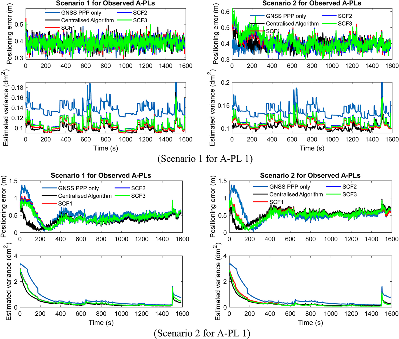
Figure 6. A-PL positioning accuracy of UNSW trial using different algorithms.

Table 2. A-PL positioning accuracy using different algorithms.

From the positioning performance comparison of scenario 1 for A-PL 1, it can be seen that the A-PL with both GNSS and inter-PL range measurements has almost the same performance in terms of positioning accuracy and smoothness as that for GNSS PPP when the A-PLs with 0.4 m GNSS PPP accuracies are observed. However, when the observed A-PLs' transmitted trajectory data deteriorates, utilising the inter-PL ranges could degrade the A-PL GNSS PPP positioning performance, as can be seen in the right figure of scenario 1 for A-PL 1. Both the centralised and distributed algorithms have to re-converge at the beginning and give slightly worse converged positioning accuracy than in the GNSS PPP-only case. The influence of inter-PL ranges on A-PL GNSS PPP positioning is further demonstrated by the comparison in scenario 2 for A-PL 1. It can be seen that by observing A-PLs with 0.4 m GNSS PPP positioning accuracies the algorithms combining GNSS PPP with inter-PL ranges achieved better converged accuracies than for the GNSS PPP-only case. There is also a tendency for a reduction in GNSS PPP convergence time, as indicated by the positioning results and estimated variances. When the trajectory data of the observed A-PLs degrades, the algorithms with both GNSS and inter-PL range measurements reduce the convergence time of GNSS PPP, except that they converge to worse positioning accuracies. Therefore, to ensure the enhancement of inter-PL ranges in practical applications, it is necessary to first check the integrity of the transmitted trajectory data. Interested readers are referred to Goel et al. (Reference Goel, Kealy, Gikas, Retscher, Toth, Brzezinska and Lohani2017) for methods of monitoring transmitted information integrity. Furthermore, when more observed A-PLs with good Geometric Dilution Of Precision (GDOP) could be assessed, there will be a reduction in convergence time for GNSS PPP when adding inter-PL range measurements.

By comparing the positioning and estimated variance results of the centralised and three SCIF-based distributed algorithms as shown in Figure 6, it can be seen that the centralised algorithm generates a smoother positioning result and has faster convergence due to the precisely tracked cross-correlations among the A-PL states. The left figure of scenario 2 for A-PL 1 illustrates this performance difference. As listed in Table 2, compared with the GNSS PPP-only case, around 20% and 10% improvement in converged positioning accuracy is achieved by the centralised and SCIF-based distributed algorithms, respectively. However, when the observed A-PLs could not provide the trajectory information with satisfactory accuracy as shown in the right figure of scenario 2 for A-PL 1, the converged accuracy of the centralised algorithm is even worse than that of the distributed algorithms. In this case, the distributed algorithms tend to be more robust in dealing with the deteriorated trajectory data of the observed A-PLs. The difference in positioning performance between the centralised and SCIF-based algorithms with scenario 1 for A-PL 1 is much smaller than that with scenario 2 for the A-PL 1. The SCIF-based algorithms can achieve almost the same positioning performance as the centralised algorithm when the GNSS PPP-only is generated by a converged solution. In the case of the three different SCIF-based distributed algorithms, all achieve almost the same positioning performance as shown by all the simulated scenarios. In principle, any one of the three SCIF-based algorithms can be used for A-PL positioning, if the slightly higher computational cost of SCIF1 is not an issue.

4.3. Analysis of predictions of orbit and satellite clock corrections

To evaluate the fitting models for short-term RTS correction predictions, the accuracy of IGC predictions with a sliding time window was investigated. The prediction errors were derived from the difference between the predicted values and their known IGC correction values during the prediction period. The periods of the fitting and prediction data were set as 10 min and 30 min, respectively. Three polynomial models with different orders including first, second and third order were investigated. The clock corrections were predicted using the model with linear and sinusoidal terms or only a linear term. For the clock prediction model, the period of the sinusoidal term was first estimated using the FFT. Other parameters involved in the prediction models for the orbit and clock corrections were estimated with a built-in “fittype” function in Matlab.

Table 3 shows one example of the prediction performance for GPS satellite PRN17. The mean and STD prediction errors represent the mean and STD value of all the prediction errors calculated with a sliding window. Since the IGC corrections are not always available, the amount of fitting data in the sliding window may vary, which has to be at least larger than five. The prediction errors only include those calculated before each IODE change or clock jump. Figure 7 shows the variation of all prediction errors. It can be seen that the worst model for orbit prediction is the one with order three. The second-order polynomial model achieves the best orbit prediction performance with the minimum mean and STD prediction errors. For satellite clock corrections, the model with linear and sinusoidal terms could obtain slightly better performance than that with only a linear term.

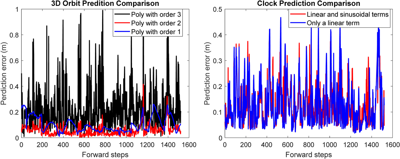
Figure 7. Correction prediction comparison.

Table 3. Mean prediction error of RTS corrections for G17.

To investigate the effect of correction prediction on A-PL positioning, it was assumed that there was one break in receiving the correction messages added to the A-PL measurements, which lasted around 10 min. The second-order polynomial and linear and sinusoidal models were used for orbit and satellite clock predictions, respectively. The A-PL positioning performance with the correction prediction was compared with the results of PPP positioning without predictions and without breaks, as shown in Figure 8. Table 4 summarises these results. The PPP positioning results obtained with correction predictions are almost the same as those without breaks, which demonstrates the effectiveness of the correction prediction models.

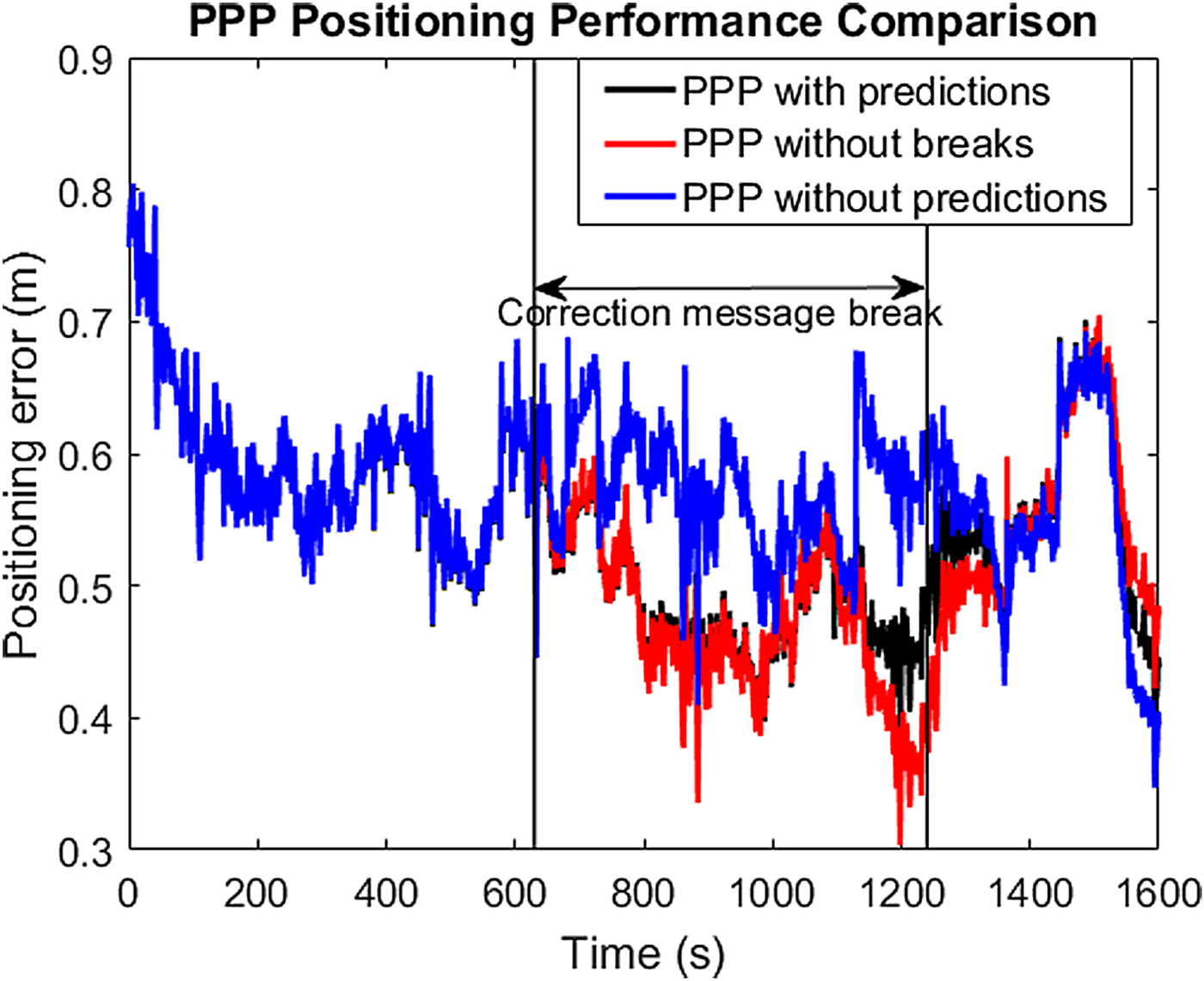
Figure 8. A-PL positioning performance.

Table 4. A-PL positioning accuracy.