


1 Introduction
Removal or displacement flow of one fluid by another is widely observed in nature. These flows also have many applications such as in the petroleum industry, coating and co-extrusion, gas assisted injection moulding, biomedical contexts (mucus, biofilms), cleaning of equipment, food processing and personal care; see Nelson & Guillot (Reference Nelson and Guillot2006), Burfoot, Middleton & Holah (Reference Burfoot, Middleton and Holah2009), Cole et al. (Reference Cole, Asteriadou, Robbins, Owen, Montague and Fryer2010). Much of the motivation for the current study comes from common multifluid flow operations present in the construction and completion of oil and gas wells, e.g. primary cementing, drilling and hydraulic fracturing. Geothermal, CO
 $_{2}$
sequestration and domestic water distribution wells are cemented using the very same techniques as in the oil and gas industry. Throughout the primary cementing process, a series of fluids are pumped down the casing, which can be tilted at any angle varying from horizontal to vertical, to remove the drilling mud and/or other in situ fluids; see Nelson & Guillot (Reference Nelson and Guillot2006). Operational failures can become highly expensive and catastrophic, as seen recently in the gulf of Mexico. For conventional resources, a water-based mud (WBM) is often used during drilling, which is miscible with cement slurry. For rapidly developing unconventional resources, the use of a miscible WBM can nonetheless cause several problems associated with swelling shales and differential sticking. These problems can be resolved by changing from a WBM to an immiscible oil-based mud (OBM) shown to improve the cement bond and thus zonal isolation; see Al Khayyat et al. (Reference Al Khayyat, Morris, Ravi and Faria1999). Whilst the displacement flow of miscible fluids has been explored in depth in the literature experimentally, computationally and analytically by Taghavi et al. (Reference Taghavi, Seon, Martinez and Frigaard2009), Taghavi, Alba & Frigaard (Reference Taghavi, Alba and Frigaard2012a
), Taghavi et al. (Reference Taghavi, Alba, Seon, Wielage-Burchard, Martinez and Frigaard2012b
), Alba, Taghavi & Frigaard (Reference Alba, Taghavi and Frigaard2013a
, Reference Alba, Taghavi and Frigaard2014), our knowledge of immiscible fluids mixing is very limited, due to the increased complexity arising from the presence of the fluids interfacial tension as well as their wetting/non-wetting characteristics when in contact with a solid geometry.
$_{2}$
sequestration and domestic water distribution wells are cemented using the very same techniques as in the oil and gas industry. Throughout the primary cementing process, a series of fluids are pumped down the casing, which can be tilted at any angle varying from horizontal to vertical, to remove the drilling mud and/or other in situ fluids; see Nelson & Guillot (Reference Nelson and Guillot2006). Operational failures can become highly expensive and catastrophic, as seen recently in the gulf of Mexico. For conventional resources, a water-based mud (WBM) is often used during drilling, which is miscible with cement slurry. For rapidly developing unconventional resources, the use of a miscible WBM can nonetheless cause several problems associated with swelling shales and differential sticking. These problems can be resolved by changing from a WBM to an immiscible oil-based mud (OBM) shown to improve the cement bond and thus zonal isolation; see Al Khayyat et al. (Reference Al Khayyat, Morris, Ravi and Faria1999). Whilst the displacement flow of miscible fluids has been explored in depth in the literature experimentally, computationally and analytically by Taghavi et al. (Reference Taghavi, Seon, Martinez and Frigaard2009), Taghavi, Alba & Frigaard (Reference Taghavi, Alba and Frigaard2012a
), Taghavi et al. (Reference Taghavi, Alba, Seon, Wielage-Burchard, Martinez and Frigaard2012b
), Alba, Taghavi & Frigaard (Reference Alba, Taghavi and Frigaard2013a
, Reference Alba, Taghavi and Frigaard2014), our knowledge of immiscible fluids mixing is very limited, due to the increased complexity arising from the presence of the fluids interfacial tension as well as their wetting/non-wetting characteristics when in contact with a solid geometry.
An important limit to our study is when the interfacial tension between the two fluids becomes very small, approaching zero. In this case, we recover a miscible flow with zero molecular diffusion or equivalently infinite Péclet number; see Petitjeans & Maxworthy (Reference Petitjeans and Maxworthy1996). Buoyant mixing and interpenetration of miscible fluids are extensively studied in the absence of an imposed flow (exchange flow configuration) using vertical and inclined pipes; e.g. see Debacq et al. (Reference Debacq, Hulin, Salin, Perrin and Hinch2003), Seon et al. (Reference Seon, Hulin, Salin, Perrin and Hinch2005), Hallez & Magnaudet (Reference Hallez and Magnaudet2008). Depending on the flow parameters, viscous, transitionary and diffusive flows may appear, characterized by the degree of interfacial instability and fluid mixing. Viscous regimes are found at nearly horizontal angles due to strong segregative buoyancy force. The interfacial waves in the form of Kelvin–Helmholtz instabilities grow at higher inclination angles leading to transitionary flows. The flow of two miscible fluids is further destabilized as the pipe is tilted towards the vertical direction which results in complete mixing in diffusive flows. Similar flows are also found for non-zero imposed velocities over a wide range of inclination angles; e.g. see Alba et al. (Reference Alba, Taghavi and Frigaard2013a , Reference Alba, Taghavi and Frigaard2014), Taghavi et al. (Reference Taghavi, Seon, Martinez and Frigaard2009, Reference Taghavi, Alba, Seon, Wielage-Burchard, Martinez and Frigaard2012b ).
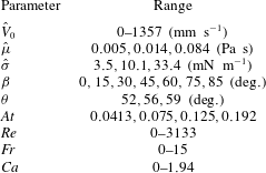
The steady, coaxial exchange flow of two immiscible fluids is studied by Kerswell (Reference Kerswell2011) revealing side by side and core–annular patterns in a vertical geometry. The spreading of the interface at long times in this configuration is governed by the balance of buoyant and viscous forces; see Matson & Hogg (Reference Matson and Hogg2012). See Zukoski (Reference Zukoski1966), Wilkinson (Reference Wilkinson1982) and Sahu & Vanka (Reference Sahu and Vanka2011), Redapangu, Vanka & Sahu (Reference Redapangu, Vanka and Sahu2012b ) for similar experimental and computational findings respectively in horizontal and/or inclined geometries. The effect of adding an imposed flow to the exchange flow of two immiscible fluids is a fairly recent topic which needs further research and analysis to be properly understood. The topic has so far only been investigated computationally using the lattice Boltzmann method (LBM) for a simplified two-dimensional (2-D) channel and square duct geometries; see Redapangu, Sahu & Vanka (Reference Redapangu, Sahu and Vanka2012a , Reference Redapangu, Sahu and Vanka2013). The significant novelties of our study are the following: We know of no other experimental study of immiscible displacement flows in the practical pipe geometry within the existing literature. Our study covers a broad range of pipe inclination angles and imposed flow rates in the density-unstable configuration. Various distinct flow regimes and instabilities have been identified in our study compared to the miscible limit, all characterized in terms of the relevant dimensionless parameters of the problem useful for industrial design. Our experimental methodology and range have been presented in § 2. In presenting the results in § 3, we first discuss the main features of the immiscible flows and then compare against existing displacement flow results of miscible fluids. Regime classification in dimensionless maps is made thereafter. The paper closes with a brief summary in § 4.
Table 1. Parameter range of our experimental study.
2 Experimental set-up and scope of study
Our experiments have been carried out in a 2 m long transparent acrylic pipe with diameter
 $\hat{D}=9.53~\text{mm}$
and thickness 3.18 mm; see figure 1(a) for a schematic representation. The pipe’s supporting structure is capable of being tilted at any angle between horizontal and vertical via a pivot. The entry condition upstream of the pipe is straightened and developed flow, which is mostly run in the laminar regime with also a few experiments carried out under the transitional regime; see table 1. In our study, the dimensional quantities are denoted with
$\hat{D}=9.53~\text{mm}$
and thickness 3.18 mm; see figure 1(a) for a schematic representation. The pipe’s supporting structure is capable of being tilted at any angle between horizontal and vertical via a pivot. The entry condition upstream of the pipe is straightened and developed flow, which is mostly run in the laminar regime with also a few experiments carried out under the transitional regime; see table 1. In our study, the dimensional quantities are denoted with
 $\hat{~}$
symbol and dimensionless quantities without. The pipe is divided into two parts, separated initially by a pneumatically operated gate valve (run at
$\hat{~}$
symbol and dimensionless quantities without. The pipe is divided into two parts, separated initially by a pneumatically operated gate valve (run at
 $103~\text{kPa}$
) which is located
$103~\text{kPa}$
) which is located
 $40~\text{cm}$
from the upper end of the pipe. The displacing fluid is a water-based solution densified by calcium chloride (CaCl
$40~\text{cm}$
from the upper end of the pipe. The displacing fluid is a water-based solution densified by calcium chloride (CaCl
 $_{2}$
) in the range
$_{2}$
) in the range
 $0{-}700~\text{g}~\text{L}^{-1}$
resulting in a density of
$0{-}700~\text{g}~\text{L}^{-1}$
resulting in a density of
 $\hat{\unicode[STIX]{x1D70C}}_{H}\in [997,1354]~\text{kg}~\text{m}^{-3}$
. Black dye (ink) with concentration
$\hat{\unicode[STIX]{x1D70C}}_{H}\in [997,1354]~\text{kg}~\text{m}^{-3}$
. Black dye (ink) with concentration
 $800~\text{mg}~\text{L}^{-1}$
is added to the displacing fluid in order to measure concentration via optical absorption. The low concentration of the dye used does not change the fluid properties. For the experiments presented in this paper, the less dense fluid is always an oil, which is used as the lower displaced fluid. In most experiments, silicone oil with density
$800~\text{mg}~\text{L}^{-1}$
is added to the displacing fluid in order to measure concentration via optical absorption. The low concentration of the dye used does not change the fluid properties. For the experiments presented in this paper, the less dense fluid is always an oil, which is used as the lower displaced fluid. In most experiments, silicone oil with density
 $\hat{\unicode[STIX]{x1D70C}}_{L}=9.18~\text{kg}~\text{m}^{-3}$
and viscosity
$\hat{\unicode[STIX]{x1D70C}}_{L}=9.18~\text{kg}~\text{m}^{-3}$
and viscosity
 $\hat{\unicode[STIX]{x1D707}}_{L}=0.005~\text{Pa}~\text{s}$
has been used. Our focus is on iso-viscous displacements, therefore, a small amount of xanthan gum thickener (
$\hat{\unicode[STIX]{x1D707}}_{L}=0.005~\text{Pa}~\text{s}$
has been used. Our focus is on iso-viscous displacements, therefore, a small amount of xanthan gum thickener (
 $245~\text{mg}~\text{L}^{-1}$
mixed for
$245~\text{mg}~\text{L}^{-1}$
mixed for
 $20$
min at
$20$
min at
 $400~\text{rpm}$
) is added to salt-water solution to match the viscosity of silicone oil. Upon rheological characterization using HR-3 Discovery Hybrid rheometer from TA Instruments, it was found that the shear-thinning effects associated with xanthan gum for the concentration given and our range of shear rate (
$400~\text{rpm}$
) is added to salt-water solution to match the viscosity of silicone oil. Upon rheological characterization using HR-3 Discovery Hybrid rheometer from TA Instruments, it was found that the shear-thinning effects associated with xanthan gum for the concentration given and our range of shear rate (
 $\hat{\dot{\unicode[STIX]{x1D6FE}}}\in [0,100]~\text{s}^{-1}$
) are negligible (
$\hat{\dot{\unicode[STIX]{x1D6FE}}}\in [0,100]~\text{s}^{-1}$
) are negligible (
 $\hat{\unicode[STIX]{x1D707}}_{H}\approx 0.004{-}0.006~\text{Pa}~\text{s}$
). Therefore, we can assume
$\hat{\unicode[STIX]{x1D707}}_{H}\approx 0.004{-}0.006~\text{Pa}~\text{s}$
). Therefore, we can assume
 $\hat{\unicode[STIX]{x1D707}}_{H}\approx \hat{\unicode[STIX]{x1D707}}_{L}\approx \hat{\unicode[STIX]{x1D707}}$
. At the start of each experiment, the gate valve is opened and the flow is driven by gravity through the use of an elevated displacing fluid tank. This ensures a smooth steady inflow.
$\hat{\unicode[STIX]{x1D707}}_{H}\approx \hat{\unicode[STIX]{x1D707}}_{L}\approx \hat{\unicode[STIX]{x1D707}}$
. At the start of each experiment, the gate valve is opened and the flow is driven by gravity through the use of an elevated displacing fluid tank. This ensures a smooth steady inflow.

Figure 1. (a) Schematic view of the experimental set-up used. (b) Snapshots of the displacement flow for
 $\unicode[STIX]{x1D6FD}=60^{\circ }$
,
$\unicode[STIX]{x1D6FD}=60^{\circ }$
,
 $\hat{V}_{0}=81.4~\text{mm}~\text{s}^{-1}$
,
$\hat{V}_{0}=81.4~\text{mm}~\text{s}^{-1}$
,
 $\hat{\unicode[STIX]{x1D70C}}_{H}=1181~\text{kg}~\text{m}^{-3}$
and
$\hat{\unicode[STIX]{x1D70C}}_{H}=1181~\text{kg}~\text{m}^{-3}$
and
 $\hat{\unicode[STIX]{x1D70C}}_{L}=918~\text{kg}~\text{m}^{-3}$
, at times
$\hat{\unicode[STIX]{x1D70C}}_{L}=918~\text{kg}~\text{m}^{-3}$
, at times
 $\hat{t}=[0.41,3.39,6.38,\ldots ,18.27,21.25]~\text{s}$
(
$\hat{t}=[0.41,3.39,6.38,\ldots ,18.27,21.25]~\text{s}$
(
 $At=0.125$
,
$At=0.125$
,
 $Re=163$
,
$Re=163$
,
 $Fr=0.75$
,
$Fr=0.75$
,
 $Ca=0.12$
,
$Ca=0.12$
,
 $\unicode[STIX]{x1D703}=56^{\circ }$
). The field of view is
$\unicode[STIX]{x1D703}=56^{\circ }$
). The field of view is
 $1950\times 9.53~\text{mm}^{2}$
. The bottommost image in panel (b) is a colour bar of concentration
$1950\times 9.53~\text{mm}^{2}$
. The bottommost image in panel (b) is a colour bar of concentration
 $C$
, with
$C$
, with
 $0$
and
$0$
and
 $1$
referring to the displaced and displacing fluids respectively. The square in image (6) indicates the location of a receding contact line where droplet shedding occurs.
$1$
referring to the displaced and displacing fluids respectively. The square in image (6) indicates the location of a receding contact line where droplet shedding occurs.
The volumetric flow rate,
 $\hat{Q}=\unicode[STIX]{x03C0}\hat{D}^{2}\hat{V}_{0}/4$
, is regulated by adjusting a needle valve located before the drain and is measured using a rotameter and a magnetic flow meter (Omega FMG91-PVDF) for the low (
$\hat{Q}=\unicode[STIX]{x03C0}\hat{D}^{2}\hat{V}_{0}/4$
, is regulated by adjusting a needle valve located before the drain and is measured using a rotameter and a magnetic flow meter (Omega FMG91-PVDF) for the low (
 $[0.84{-}8.6]\times 10^{-6}~\text{m}^{3}~\text{s}^{-1}$
) and high (
$[0.84{-}8.6]\times 10^{-6}~\text{m}^{3}~\text{s}^{-1}$
) and high (
 $[0.42-8.2]\times 10^{-5}~\text{m}^{3}~\text{s}^{-1}$
) ranges of the imposed flow respectively. Here,
$[0.42-8.2]\times 10^{-5}~\text{m}^{3}~\text{s}^{-1}$
) ranges of the imposed flow respectively. Here,
 $\hat{V}_{0}$
is the mean imposed velocity. In an experiment, the two fluids are initially filled above and below the gate valve correspondingly. The pipe is back-lit using light-emitting diode (LED) strips. A diffusive layer is placed between LED strips and pipe to improve light homogeneity. The optical measurement method consists of acquiring images of the pipe using a high-speed black-and-white digital camera (Basler Ace acA2040-90um CMOS,
$\hat{V}_{0}$
is the mean imposed velocity. In an experiment, the two fluids are initially filled above and below the gate valve correspondingly. The pipe is back-lit using light-emitting diode (LED) strips. A diffusive layer is placed between LED strips and pipe to improve light homogeneity. The optical measurement method consists of acquiring images of the pipe using a high-speed black-and-white digital camera (Basler Ace acA2040-90um CMOS,
 $2048^{2}$
pixels), with
$2048^{2}$
pixels), with
 $4096$
grey scale levels. This allows us to analyse a reasonably wide range of concentrations. The camera covers the whole 2-m length of the pipe using a high-resolution lens (
$4096$
grey scale levels. This allows us to analyse a reasonably wide range of concentrations. The camera covers the whole 2-m length of the pipe using a high-resolution lens (
 $16~\text{mm}$
F/1.8 C-mount) and records images at a rate of
$16~\text{mm}$
F/1.8 C-mount) and records images at a rate of
 $8{-}90~\text{Hz}$
, depending on the imposed flow rate. The grey scale images obtained from the camera have been converted to colour pictures using a MATLAB image processing code for improved presentation of the results. The surface tension between the two fluids is measured with a tensiometer (Sigma Force Tensiometer 701 from Biolin Scientific Inc.). The device has been successfully calibrated against air–water (
$8{-}90~\text{Hz}$
, depending on the imposed flow rate. The grey scale images obtained from the camera have been converted to colour pictures using a MATLAB image processing code for improved presentation of the results. The surface tension between the two fluids is measured with a tensiometer (Sigma Force Tensiometer 701 from Biolin Scientific Inc.). The device has been successfully calibrated against air–water (
 $\hat{\unicode[STIX]{x1D70E}}=72.9~\text{mN}~\text{m}^{-1}$
) and air–silicone oil (
$\hat{\unicode[STIX]{x1D70E}}=72.9~\text{mN}~\text{m}^{-1}$
) and air–silicone oil (
 $\hat{\unicode[STIX]{x1D70E}}=22.1~\text{mN}~\text{m}^{-1}$
).
$\hat{\unicode[STIX]{x1D70E}}=22.1~\text{mN}~\text{m}^{-1}$
).
An ultrasonic Doppler velocimeter (UDV – model DOP4000 from Signal Processing SA), has also been used in order to measure local velocity profiles of the flow, gaining additional insight into the dynamics of the flow. The measurements are made
 $850~\text{mm}$
downstream of the gate valve. For the tracer, polyamide seeding particles (PSP) with a mean particle diameter of
$850~\text{mm}$
downstream of the gate valve. For the tracer, polyamide seeding particles (PSP) with a mean particle diameter of
 $50$
microns and density close to that of fluid pairs (
$50$
microns and density close to that of fluid pairs (
 $\hat{\unicode[STIX]{x1D70C}}_{PSP}=1030~\text{kg}~\text{m}^{-3}$
) are used to ensure they stay neutrally buoyant within the flow (Stokes settling velocity of the particles
$\hat{\unicode[STIX]{x1D70C}}_{PSP}=1030~\text{kg}~\text{m}^{-3}$
) are used to ensure they stay neutrally buoyant within the flow (Stokes settling velocity of the particles
 ${\approx}0.1~\text{mm}~\text{s}^{-1}$
without considering hindrance and wall effects; see Cook, Bertozzi & Hosoi (Reference Cook, Bertozzi and Hosoi2008) for details). Note that in our previous studies for miscible fluids such as in Alba et al. (Reference Alba, Taghavi and Frigaard2013a
), a volumetric PSP concentration of
${\approx}0.1~\text{mm}~\text{s}^{-1}$
without considering hindrance and wall effects; see Cook, Bertozzi & Hosoi (Reference Cook, Bertozzi and Hosoi2008) for details). Note that in our previous studies for miscible fluids such as in Alba et al. (Reference Alba, Taghavi and Frigaard2013a
), a volumetric PSP concentration of
 $0.2~\text{g}~\text{L}^{-1}$
has been used in the UDV measurements. However, when mixed with an oil, this low concentration of PSP will not provide an acceptable UDV echo. Thus, we needed to increase the concentration up to
$0.2~\text{g}~\text{L}^{-1}$
has been used in the UDV measurements. However, when mixed with an oil, this low concentration of PSP will not provide an acceptable UDV echo. Thus, we needed to increase the concentration up to
 $0.5~\text{g}~\text{L}^{-1}$
(in both fluids) to overcome this issue. The concentration used was found to have a negligible effect on the viscosity of our solutions. The measuring volume of the probe has a cylindrical shape. The axial resolution of UDV within the depth of our fluids is approximately
$0.5~\text{g}~\text{L}^{-1}$
(in both fluids) to overcome this issue. The concentration used was found to have a negligible effect on the viscosity of our solutions. The measuring volume of the probe has a cylindrical shape. The axial resolution of UDV within the depth of our fluids is approximately
 $0.128~\text{mm}$
and the lateral resolution is equal to the transducer diameter (
$0.128~\text{mm}$
and the lateral resolution is equal to the transducer diameter (
 $8~\text{mm}$
), slightly varying with depth. A
$8~\text{mm}$
), slightly varying with depth. A
 $4$
-MHz transducer has been used in our measurements. The probe was mounted at an angle
$4$
-MHz transducer has been used in our measurements. The probe was mounted at an angle
 ${\approx}75^{\circ }$
relative to the axis of the pipe, selected to balance a good signal to noise ratio with small ultrasonic signal reflections; see Brunone & Berni (Reference Brunone and Berni2010) for details. The UDV measures the flow velocity projection on the ultrasound beam, essentially giving the axial velocity across the pipe. In a typical experimental sequence, we would fix the pipe inclination and fluid pairs and then run a number of experiments at increasing fixed flow rates while capturing flow visualization and velocimetry data.
${\approx}75^{\circ }$
relative to the axis of the pipe, selected to balance a good signal to noise ratio with small ultrasonic signal reflections; see Brunone & Berni (Reference Brunone and Berni2010) for details. The UDV measures the flow velocity projection on the ultrasound beam, essentially giving the axial velocity across the pipe. In a typical experimental sequence, we would fix the pipe inclination and fluid pairs and then run a number of experiments at increasing fixed flow rates while capturing flow visualization and velocimetry data.
An analysis of the flow suggests that 7 dimensional parameters may govern the immiscible flow; see table 1 and also Alba et al. (Reference Alba, Taghavi and Frigaard2013a
) for miscible limit analysis. The dimensionless numbers associated with the geometry are pipe inclination angle,
 $\unicode[STIX]{x1D6FD}$
, and aspect ratio,
$\unicode[STIX]{x1D6FD}$
, and aspect ratio,
 $\unicode[STIX]{x1D6FF}=\hat{D}/\hat{L}$
, where
$\unicode[STIX]{x1D6FF}=\hat{D}/\hat{L}$
, where
 $\hat{L}$
is the length of the pipe. Industrially, we are interested in pipes with small aspect ratio i.e.
$\hat{L}$
is the length of the pipe. Industrially, we are interested in pipes with small aspect ratio i.e.
 $\unicode[STIX]{x1D6FF}\ll 1$
; see Nelson & Guillot (Reference Nelson and Guillot2006). Given our experimental set-up, we have
$\unicode[STIX]{x1D6FF}\ll 1$
; see Nelson & Guillot (Reference Nelson and Guillot2006). Given our experimental set-up, we have
 $\unicode[STIX]{x1D6FF}=0.00476$
. A third dimensionless parameter is the Reynolds number,
$\unicode[STIX]{x1D6FF}=0.00476$
. A third dimensionless parameter is the Reynolds number,
 $Re=\hat{V}_{0}\hat{D}/\hat{\unicode[STIX]{x1D708}}$
, where
$Re=\hat{V}_{0}\hat{D}/\hat{\unicode[STIX]{x1D708}}$
, where
 $\hat{\unicode[STIX]{x1D708}}$
is defined using the mean density
$\hat{\unicode[STIX]{x1D708}}$
is defined using the mean density
 $\hat{\unicode[STIX]{x1D70C}}=(\hat{\unicode[STIX]{x1D70C}}_{L}+\hat{\unicode[STIX]{x1D70C}}_{H})/2$
and the common viscosity of the two fluids,
$\hat{\unicode[STIX]{x1D70C}}=(\hat{\unicode[STIX]{x1D70C}}_{L}+\hat{\unicode[STIX]{x1D70C}}_{H})/2$
and the common viscosity of the two fluids,
 $\hat{\unicode[STIX]{x1D707}}$
. The fourth dimensionless parameter is the Atwood number defined as
$\hat{\unicode[STIX]{x1D707}}$
. The fourth dimensionless parameter is the Atwood number defined as
 $At=(\hat{\unicode[STIX]{x1D70C}}_{H}-\hat{\unicode[STIX]{x1D70C}}_{L})/(\hat{\unicode[STIX]{x1D70C}}_{H}+\hat{\unicode[STIX]{x1D70C}}_{L})$
, representing a dimensionless density difference. For this study,
$At=(\hat{\unicode[STIX]{x1D70C}}_{H}-\hat{\unicode[STIX]{x1D70C}}_{L})/(\hat{\unicode[STIX]{x1D70C}}_{H}+\hat{\unicode[STIX]{x1D70C}}_{L})$
, representing a dimensionless density difference. For this study,
 $At>0$
since
$At>0$
since
 $\hat{\unicode[STIX]{x1D70C}}_{H}>\hat{\unicode[STIX]{x1D70C}}_{L}$
. Our experiments are mostly performed for
$\hat{\unicode[STIX]{x1D70C}}_{H}>\hat{\unicode[STIX]{x1D70C}}_{L}$
. Our experiments are mostly performed for
 $At=0.075,0.125$
. Since
$At=0.075,0.125$
. Since
 $At$
can be larger than
$At$
can be larger than
 $0.1$
, the Boussinesq approximation may not be entirely valid; see Sundén & Brebbia (Reference Sundén and Brebbia2006). The significance of inertial to buoyant stresses is captured by the densimetric Froude number,
$0.1$
, the Boussinesq approximation may not be entirely valid; see Sundén & Brebbia (Reference Sundén and Brebbia2006). The significance of inertial to buoyant stresses is captured by the densimetric Froude number,
 $Fr=\hat{V}_{0}/\sqrt{At{\hat{g}}\hat{D}}$
, where
$Fr=\hat{V}_{0}/\sqrt{At{\hat{g}}\hat{D}}$
, where
 ${\hat{g}}$
is the gravitational acceleration. Finally, since our fluids are immiscible, two more dimensionless numbers become relevant, namely the capillary number, defined as
${\hat{g}}$
is the gravitational acceleration. Finally, since our fluids are immiscible, two more dimensionless numbers become relevant, namely the capillary number, defined as
 $Ca=\hat{\unicode[STIX]{x1D707}}\hat{V}_{0}/\hat{\unicode[STIX]{x1D70E}}$
, and the contact angle between the two fluids,
$Ca=\hat{\unicode[STIX]{x1D707}}\hat{V}_{0}/\hat{\unicode[STIX]{x1D70E}}$
, and the contact angle between the two fluids,
 $\unicode[STIX]{x1D703}$
. Motivated by the primary cementing process of the wells drilled using OBM, we consider the case that the water-based displacing fluid is wetting and the oil-based displaced one is non-wetting in the presence of a solid boundary. In summary, providing
$\unicode[STIX]{x1D703}$
. Motivated by the primary cementing process of the wells drilled using OBM, we consider the case that the water-based displacing fluid is wetting and the oil-based displaced one is non-wetting in the presence of a solid boundary. In summary, providing
 $\unicode[STIX]{x1D6FF}\ll 1$
the important dimensionless parameters of the problem reduce to six, namely
$\unicode[STIX]{x1D6FF}\ll 1$
the important dimensionless parameters of the problem reduce to six, namely
 $\unicode[STIX]{x1D6FD}$
,
$\unicode[STIX]{x1D6FD}$
,
 $At$
,
$At$
,
 $Re$
,
$Re$
,
 $Fr$
,
$Fr$
,
 $Ca$
and
$Ca$
and
 $\unicode[STIX]{x1D703}$
. The range of dimensional and dimensionless parameters is shown in table 1. Evidently, we are able to cover a wide range of these parameters with our experiments (total of 168). In presenting our results, both dimensional and dimensionless quantities are provided for convenience. Most of the experiments shown are conducted with the parameters
$\unicode[STIX]{x1D703}$
. The range of dimensional and dimensionless parameters is shown in table 1. Evidently, we are able to cover a wide range of these parameters with our experiments (total of 168). In presenting our results, both dimensional and dimensionless quantities are provided for convenience. Most of the experiments shown are conducted with the parameters
 $\hat{\unicode[STIX]{x1D707}}=0.005~\text{Pa}~\text{s}$
,
$\hat{\unicode[STIX]{x1D707}}=0.005~\text{Pa}~\text{s}$
,
 $\hat{\unicode[STIX]{x1D70E}}=3.5~\text{mN}~\text{m}^{-1}$
,
$\hat{\unicode[STIX]{x1D70E}}=3.5~\text{mN}~\text{m}^{-1}$
,
 $\unicode[STIX]{x1D703}=56^{\circ }$
and
$\unicode[STIX]{x1D703}=56^{\circ }$
and
 $At=0.075,~0.125$
unless otherwise stated.
$At=0.075,~0.125$
unless otherwise stated.
3 Results
We now present our experimental results. In § 3.1, we first give a detailed description of the main features observed in our immiscible displacement flow experiments and then compare them against existing results for miscible fluids. The variations in measured displacing front velocity, important in estimating the displacement efficiency, is studied in § 3.2. The immiscible effects are studied in § 3.3 for various fluid pairs. The behaviour of the trailing displacement front is discussed in § 3.4. In § 3.5, we classify the flow regimes observed, approximating the boundaries in terms of the dimensionless parameters of the problem.
3.1 Immiscible displacement flows: main features
We first aim to present a typical immiscible displacement flow. Figure 1(b) shows snapshots of an experiment for CaCl
 $_{2}$
–water displacing silicone oil. The fluids are initially separated by a gate valve (green rectangle). Upon opening the gate valve, the light fluid is instantaneously pushed in the downstream direction (instantaneous displacement). In other words, there is no flow of the light displaced layer observed upstream of the gate valve (zero back flow). The formation of a narrow displacing layer towards the bottom wall is evident. The droplets of silicone oil are located closer to the trailing front. Note that the trailing front is the one driven by the light fluid, as opposed to the heavy fluid, which is referred to as displacing front. Another feature of the flow prevalently observed in the immiscible experiments is the formation of interfacial kinks. These kinks, amplitude of which stay rather constant throughout the experiment, originate from strong interfacial instabilities at early times. Figure 2 shows the short time behaviour of the flow more clearly. After opening the gate valve, a rather (stable) stratified interface forms; figure 2(3). Due to the highly unstable nature of this interface, perturbations grow very quickly over time, reaching the top and/or bottom walls of the pipe; figure 2(8). Via tracking the interface modulations, we found that the interfacial kinks observed at later times in figure 1(b) result from these very early time instabilities.
$_{2}$
–water displacing silicone oil. The fluids are initially separated by a gate valve (green rectangle). Upon opening the gate valve, the light fluid is instantaneously pushed in the downstream direction (instantaneous displacement). In other words, there is no flow of the light displaced layer observed upstream of the gate valve (zero back flow). The formation of a narrow displacing layer towards the bottom wall is evident. The droplets of silicone oil are located closer to the trailing front. Note that the trailing front is the one driven by the light fluid, as opposed to the heavy fluid, which is referred to as displacing front. Another feature of the flow prevalently observed in the immiscible experiments is the formation of interfacial kinks. These kinks, amplitude of which stay rather constant throughout the experiment, originate from strong interfacial instabilities at early times. Figure 2 shows the short time behaviour of the flow more clearly. After opening the gate valve, a rather (stable) stratified interface forms; figure 2(3). Due to the highly unstable nature of this interface, perturbations grow very quickly over time, reaching the top and/or bottom walls of the pipe; figure 2(8). Via tracking the interface modulations, we found that the interfacial kinks observed at later times in figure 1(b) result from these very early time instabilities.
Upon comparing figure 1(b)(3) and (4), one may find that some of these kinks have disappeared. However, this is not really the case and the waves may rather coalesce over time. Figure 3 shows such wave coalescence behaviour more clearly over a higher number of snapshots. The rectangular regions in figure 3(a) highlight merging of waves. It is useful to define a cross-sectional-averaged concentration,
 $\bar{C}_{{\hat{y}}}(\hat{x},\hat{t})$
to assess how much displacing and/or displaced fluids exist in a given streamwise location,
$\bar{C}_{{\hat{y}}}(\hat{x},\hat{t})$
to assess how much displacing and/or displaced fluids exist in a given streamwise location,
 $\hat{x}$
, at time
$\hat{x}$
, at time
 $\hat{t}$
. Note that due to our back-lighting technique, the concentration values,
$\hat{t}$
. Note that due to our back-lighting technique, the concentration values,
 $C$
, captured by the camera are already averaged in the transverse
$C$
, captured by the camera are already averaged in the transverse
 $\hat{z}$
direction i.e.
$\hat{z}$
direction i.e.
 $C=C(\hat{x},{\hat{y}},\hat{t})$
only. Figure 3(b) shows
$C=C(\hat{x},{\hat{y}},\hat{t})$
only. Figure 3(b) shows
 $\bar{C}_{{\hat{y}}}(\hat{x},\hat{t})$
for the same snapshots as in part (a) in order to indicate and track the location of waves more accurately. Coalescence of waves 5 and 6 is clear from figure 3(b). Waves 2 and 3 have also approached towards one another. The wave coalescence behaviour has, in fact, been commonly observed in many other studies related to the prediction of instability, interface pinch off and slugging onset at immiscible interfaces; e.g. see Lin & Hanratty (Reference Lin and Hanratty1986), Woods & Hanratty (Reference Woods and Hanratty1996), Hanyang & Liejin (Reference Hanyang and Liejin2008).
$\bar{C}_{{\hat{y}}}(\hat{x},\hat{t})$
for the same snapshots as in part (a) in order to indicate and track the location of waves more accurately. Coalescence of waves 5 and 6 is clear from figure 3(b). Waves 2 and 3 have also approached towards one another. The wave coalescence behaviour has, in fact, been commonly observed in many other studies related to the prediction of instability, interface pinch off and slugging onset at immiscible interfaces; e.g. see Lin & Hanratty (Reference Lin and Hanratty1986), Woods & Hanratty (Reference Woods and Hanratty1996), Hanyang & Liejin (Reference Hanyang and Liejin2008).
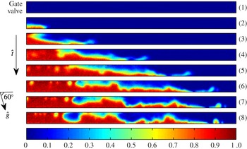
Figure 2. Snapshots of the displacement flow in figure 1(b) at early times
 $\hat{t}=[0,0.086,0.172,0.258,\ldots ,0.516,0.602]~\text{s}$
showing the growth of interfacial instability. The domain covers
$\hat{t}=[0,0.086,0.172,0.258,\ldots ,0.516,0.602]~\text{s}$
showing the growth of interfacial instability. The domain covers
 $0~\text{mm}<\hat{x}<245~\text{mm}$
. The bottommost image is a colour bar of concentration
$0~\text{mm}<\hat{x}<245~\text{mm}$
. The bottommost image is a colour bar of concentration
 $C$
, with
$C$
, with
 $0$
and
$0$
and
 $1$
referring to the displaced and displacing fluids respectively.
$1$
referring to the displaced and displacing fluids respectively.

Figure 3. (a) Snapshots of the concentration for the displacement flow shown in figure 1(b) at times
 $\hat{t}=[5,5.7,6.4,7.1,7.8]~\text{s}$
. The domain covers 600 mm
$\hat{t}=[5,5.7,6.4,7.1,7.8]~\text{s}$
. The domain covers 600 mm
 ${<}\hat{x}<1350~\text{mm}$
. (b) Cross-sectional-averaged profiles of the concentration corresponding to snapshots in (a).
${<}\hat{x}<1350~\text{mm}$
. (b) Cross-sectional-averaged profiles of the concentration corresponding to snapshots in (a).

Figure 4. The dependency of the Richardson number,
 $Ri$
, on wavenumber,
$Ri$
, on wavenumber,
 $\hat{k}$
, for the early time (figure 2) and long-time (figure 3) phases of the displacement flow. The dashed line indicates
$\hat{k}$
, for the early time (figure 2) and long-time (figure 3) phases of the displacement flow. The dashed line indicates
 $Ri=1$
predicting the onset of Kelvin–Helmholtz instabilities as found by Funada & Joseph (Reference Funada and Joseph2001).
$Ri=1$
predicting the onset of Kelvin–Helmholtz instabilities as found by Funada & Joseph (Reference Funada and Joseph2001).
The early time snapshots in figure 2 suggest large speeds and strong shearing between the heavy and light fluid layers making the interface potentially susceptible to Kelvin–Helmholtz instabilities. Building up on the pioneering work of Thorpe (Reference Thorpe1969), through a robust stability analysis Funada & Joseph (Reference Funada and Joseph2001) found that the onset of Kelvin–Helmholtz instability in an immiscible two-layered system is independent of viscosity and can be captured through a Richardson number,
 $Ri$
, defined as
$Ri$
, defined as
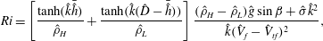 $$\begin{eqnarray}Ri=\left[\frac{\tanh (\hat{k}\bar{{\hat{h}}})}{\hat{\unicode[STIX]{x1D70C}}_{H}}+\frac{\tanh (\hat{k}(\hat{D}-\bar{{\hat{h}}}))}{\hat{\unicode[STIX]{x1D70C}}_{L}}\right]\frac{(\hat{\unicode[STIX]{x1D70C}}_{H}-\hat{\unicode[STIX]{x1D70C}}_{L}){\hat{g}}\sin \unicode[STIX]{x1D6FD}+\hat{\unicode[STIX]{x1D70E}}\hat{k}^{2}}{\hat{k}(\hat{V}_{f}-\hat{V}_{tf})^{2}},\end{eqnarray}$$
where
 $\bar{{\hat{h}}}$
is the average interface height,
$\bar{{\hat{h}}}$
is the average interface height,
 $\hat{k}$
the wavenumber as in interface perturbation
$\hat{k}$
the wavenumber as in interface perturbation
 ${\hat{h}}=\hat{A}\text{e}^{\text{i}\hat{k}\hat{x}+(\hat{\unicode[STIX]{x1D70E}}_{R}+\text{i}\hat{\unicode[STIX]{x1D70E}}_{I})\hat{t}}$
(
${\hat{h}}=\hat{A}\text{e}^{\text{i}\hat{k}\hat{x}+(\hat{\unicode[STIX]{x1D70E}}_{R}+\text{i}\hat{\unicode[STIX]{x1D70E}}_{I})\hat{t}}$
(
 $\hat{A}$
being amplitude and
$\hat{A}$
being amplitude and
 $\hat{\unicode[STIX]{x1D70E}}_{R}$
and
$\hat{\unicode[STIX]{x1D70E}}_{R}$
and
 $\hat{\unicode[STIX]{x1D70E}}_{I}$
the growth rate and wave speed respectively) and
$\hat{\unicode[STIX]{x1D70E}}_{I}$
the growth rate and wave speed respectively) and
 $\hat{V}_{f}$
and
$\hat{V}_{f}$
and
 $\hat{V}_{tf}$
the displacing and trailing front velocities which we will explain in detail how to measure in § 3.2. The Richardson number, in a sense, is the ratio of stabilizing potential energy of gravity and surface tension to destabilizing kinetic energy at the interface. Therefore,
$\hat{V}_{tf}$
the displacing and trailing front velocities which we will explain in detail how to measure in § 3.2. The Richardson number, in a sense, is the ratio of stabilizing potential energy of gravity and surface tension to destabilizing kinetic energy at the interface. Therefore,
 $Ri<1$
represents unstable flow; see Funada & Joseph (Reference Funada and Joseph2001). Figure 4 shows the variation of
$Ri<1$
represents unstable flow; see Funada & Joseph (Reference Funada and Joseph2001). Figure 4 shows the variation of
 $Ri$
with
$Ri$
with
 $\hat{k}$
for stratified situation shown in figure 2(3) assuming
$\hat{k}$
for stratified situation shown in figure 2(3) assuming
 $\bar{{\hat{h}}}\approx 0.5\hat{D}$
. The Richardson number can be less than 1 over a large range of wavenumbers with the minimum happening at
$\bar{{\hat{h}}}\approx 0.5\hat{D}$
. The Richardson number can be less than 1 over a large range of wavenumbers with the minimum happening at
 $\hat{k}\approx 793~\text{m}^{-1}$
. Note that this value of
$\hat{k}\approx 793~\text{m}^{-1}$
. Note that this value of
 $\hat{k}$
corresponds to a wavelength of
$\hat{k}$
corresponds to a wavelength of
 $\hat{\unicode[STIX]{x1D706}}=2\unicode[STIX]{x03C0}/\hat{k}\approx 7.92~\text{mm}$
which is comparable to the instabilities observed in the figure 2 snapshots. Given
$\hat{\unicode[STIX]{x1D706}}=2\unicode[STIX]{x03C0}/\hat{k}\approx 7.92~\text{mm}$
which is comparable to the instabilities observed in the figure 2 snapshots. Given
 $\bar{{\hat{h}}}$
,
$\bar{{\hat{h}}}$
,
 $\hat{V}_{f}$
and
$\hat{V}_{f}$
and
 $\hat{V}_{tf}$
of the flow at longer times (figure 3) we can similarly calculate the Richardson number which is also added to figure 4. It can be seen that
$\hat{V}_{tf}$
of the flow at longer times (figure 3) we can similarly calculate the Richardson number which is also added to figure 4. It can be seen that
 $Ri$
(which is much larger than early time values) can be marginally less than 1 (unstable). Moreover, the instability at long times occurs over a much narrower range of wavenumber compared to the early times. Finally, note that in interpreting the stability results, while the linear theory may predict unbounded exponential growth of infinitesimally small perturbations, once they grow over time the nonlinear terms become important, modifying the dynamics of the flow; see Stuart (Reference Stuart1960) and Drazin & Reid (Reference Drazin and Reid2004).
$Ri$
(which is much larger than early time values) can be marginally less than 1 (unstable). Moreover, the instability at long times occurs over a much narrower range of wavenumber compared to the early times. Finally, note that in interpreting the stability results, while the linear theory may predict unbounded exponential growth of infinitesimally small perturbations, once they grow over time the nonlinear terms become important, modifying the dynamics of the flow; see Stuart (Reference Stuart1960) and Drazin & Reid (Reference Drazin and Reid2004).

Figure 5. Snapshots of the displacement flow in figure 1(b) at times
 $\hat{t}=[7.91,8.27,8.63,\ldots ,10.07,10.43]~\text{s}$
showing droplet shedding (pearling) in the vicinity of the highlighted rectangular region in image (1). The domain covers
$\hat{t}=[7.91,8.27,8.63,\ldots ,10.07,10.43]~\text{s}$
showing droplet shedding (pearling) in the vicinity of the highlighted rectangular region in image (1). The domain covers
 $432~\text{mm}<\hat{x}<805~\text{mm}$
. The bottommost image is a colour bar of concentration
$432~\text{mm}<\hat{x}<805~\text{mm}$
. The bottommost image is a colour bar of concentration
 $C$
, with
$C$
, with
 $0$
and
$0$
and
 $1$
referring to the displaced and displacing fluids respectively.
$1$
referring to the displaced and displacing fluids respectively.
Although the intensity of Kelvin–Helmholtz instabilities at long times is reduced, there are still other modes of instability active in the flow. The snapshots in figure 1(b)(5)–(8) exhibit continuous droplet shedding at a receding contact line. In the literature, see e.g. Eres, Schwartz & Roy (Reference Eres, Schwartz and Roy2000), Podgorski, Flesselles & Limat (Reference Podgorski, Flesselles and Limat2001), such droplet shedding, often referred to as pearling, is associated with surface-tension-driven Rayleigh-type instabilities. Figure 5 provides a closer look into the pearling mechanism and its formation over a rather short period of time. The thin film of light silicone fluid is pinched off in snapshot (4) creating advancing and receding contact lines (fronts). Snapshots (5)–(8) afterwards reveal constant detachment of droplets from the receding front. The detached droplets are then merged into the upstream advancing front. In a novel work, Podgorski et al. (Reference Podgorski, Flesselles and Limat2001) showed that for a droplet of silicone oil, the transition to pearling regime occurs if its speed exceeds the following critical value:
 $$\begin{eqnarray}\hat{V}_{cr}=2\unicode[STIX]{x1D705}\hat{\unicode[STIX]{x1D70E}}\unicode[STIX]{x1D703}_{r}^{3}/\hat{\unicode[STIX]{x1D707}},\end{eqnarray}$$
where
 $\unicode[STIX]{x1D705}$
is a constant that for 0.005 Pa s silicone oil can be calculated as
$\unicode[STIX]{x1D705}$
is a constant that for 0.005 Pa s silicone oil can be calculated as
 $\unicode[STIX]{x1D705}\approx 0.01$
; see Podgorski et al. (Reference Podgorski, Flesselles and Limat2001). In (3.2),
$\unicode[STIX]{x1D705}\approx 0.01$
; see Podgorski et al. (Reference Podgorski, Flesselles and Limat2001). In (3.2),
 $\unicode[STIX]{x1D703}_{r}$
is the receding contact angle prior to the droplet breakup and shedding which from figure 5(5) can be assumed to be
$\unicode[STIX]{x1D703}_{r}$
is the receding contact angle prior to the droplet breakup and shedding which from figure 5(5) can be assumed to be
 $\unicode[STIX]{x1D703}_{r}\approx \unicode[STIX]{x03C0}/2$
. Equation (3.2) then predicts
$\unicode[STIX]{x1D703}_{r}\approx \unicode[STIX]{x03C0}/2$
. Equation (3.2) then predicts
 $\hat{V}_{cr}$
to be of order
$\hat{V}_{cr}$
to be of order
 $50~\text{mm}~\text{s}^{-1}$
. Through measurement of the receding contact line speed in figure 5, we found
$50~\text{mm}~\text{s}^{-1}$
. Through measurement of the receding contact line speed in figure 5, we found
 $\hat{V}\approx 95.6~\text{mm}~\text{s}^{-1}$
suggesting that Rayleigh instability can indeed be the responsible mechanism for the pearling phenomenon observed in our experiments; see also figure 6(b). In most of our experiments, the pearling was noticed to occur at receding contact lines forming after an interface pinch off. Just after pinch off, the dynamic contact angle at receding front can become very small and, according to (3.2), the interface becomes susceptible to surface-tension-driven instabilities given that it is advancing fast enough. Formula (3.2) has been derived for a droplet exposed to air (not liquid–liquid system). However, Espin & Kumar (Reference Espin and Kumar2017) recently found that an external shear on the droplet surface does not significantly change the pearling transition critical speed. Finally, note that due to the given density-unstable configuration, the Rayleigh–Taylor instability may also be potentially present in our experiments. However, we might neglect its effect at inclination angles away from the vertical direction. In the discussion to follow in this section, we will explore the role of surface tension on Rayleigh–Taylor instability in detail.
$\hat{V}\approx 95.6~\text{mm}~\text{s}^{-1}$
suggesting that Rayleigh instability can indeed be the responsible mechanism for the pearling phenomenon observed in our experiments; see also figure 6(b). In most of our experiments, the pearling was noticed to occur at receding contact lines forming after an interface pinch off. Just after pinch off, the dynamic contact angle at receding front can become very small and, according to (3.2), the interface becomes susceptible to surface-tension-driven instabilities given that it is advancing fast enough. Formula (3.2) has been derived for a droplet exposed to air (not liquid–liquid system). However, Espin & Kumar (Reference Espin and Kumar2017) recently found that an external shear on the droplet surface does not significantly change the pearling transition critical speed. Finally, note that due to the given density-unstable configuration, the Rayleigh–Taylor instability may also be potentially present in our experiments. However, we might neglect its effect at inclination angles away from the vertical direction. In the discussion to follow in this section, we will explore the role of surface tension on Rayleigh–Taylor instability in detail.

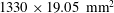
Figure 6. Change in iso-viscous displacement flow with
 $\unicode[STIX]{x1D6FD}$
. (a) For miscible fluids (salt-water displacing water) of Alba et al. (Reference Alba, Taghavi and Frigaard2013a
) (
$\unicode[STIX]{x1D6FD}$
. (a) For miscible fluids (salt-water displacing water) of Alba et al. (Reference Alba, Taghavi and Frigaard2013a
) (
 $At=0.0035$
,
$At=0.0035$
,
 $Re\approx 726$
,
$Re\approx 726$
,
 $Fr\approx 1.48$
,
$Fr\approx 1.48$
,
 $Ca=\infty$
). The field of view is
$Ca=\infty$
). The field of view is
 $1330\times 19.05~\text{mm}^{2}$
located 1740 mm downstream of the gate valve. (b) For immiscible fluids (current study) obtained for
$1330\times 19.05~\text{mm}^{2}$
located 1740 mm downstream of the gate valve. (b) For immiscible fluids (current study) obtained for
 $\hat{\unicode[STIX]{x1D70C}}_{H}=1181~\text{kg}~\text{m}^{-3}$
,
$\hat{\unicode[STIX]{x1D70C}}_{H}=1181~\text{kg}~\text{m}^{-3}$
,
 $\hat{\unicode[STIX]{x1D70C}}_{L}=918~\text{kg}~\text{m}^{-3}$
and approximately close imposed flow rates
$\hat{\unicode[STIX]{x1D70C}}_{L}=918~\text{kg}~\text{m}^{-3}$
and approximately close imposed flow rates
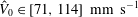 $\hat{V}_{0}\in [71,114]~\text{mm}~\text{s}^{-1}$
(
$\hat{V}_{0}\in [71,114]~\text{mm}~\text{s}^{-1}$
(
 $At=0.125$
,
$At=0.125$
,
 $Re\in [146,247]$
,
$Re\in [146,247]$
,
 $Fr\in [0.66,1.05]$
,
$Fr\in [0.66,1.05]$
,
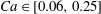 $Ca\in [0.06,0.25]$
,
$Ca\in [0.06,0.25]$
,
 $\unicode[STIX]{x1D703}=56^{\circ }$
). The field of view is
$\unicode[STIX]{x1D703}=56^{\circ }$
). The field of view is
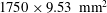 $1750\times 9.53~\text{mm}^{2}$
. The colour bar at the top left of the figures shows the corresponding concentration value,
$1750\times 9.53~\text{mm}^{2}$
. The colour bar at the top left of the figures shows the corresponding concentration value,
 $C$
, with
$C$
, with
 $0$
referring to the pure displaced fluid and
$0$
referring to the pure displaced fluid and
 $1$
to the pure displacing fluid.
$1$
to the pure displacing fluid.
Let us now examine how the immiscible experiments compare against our previous miscible experiments in Alba et al. (Reference Alba, Taghavi and Frigaard2013a
) over a large range of inclination angles. Figure 6(a) shows the snapshots of experiments by Alba et al. (Reference Alba, Taghavi and Frigaard2013a
) for miscible fluids (salt-water displacing water) revealing viscous (
 $\unicode[STIX]{x1D6FD}=85^{\circ }$
), transitionary (
$\unicode[STIX]{x1D6FD}=85^{\circ }$
), transitionary (
 $\unicode[STIX]{x1D6FD}=30^{\circ },45^{\circ },60^{\circ },70^{\circ }$
) and diffusive (
$\unicode[STIX]{x1D6FD}=30^{\circ },45^{\circ },60^{\circ },70^{\circ }$
) and diffusive (
 $\unicode[STIX]{x1D6FD}=0^{\circ }$
) flows. The observed interfacial mixing, which is increased as the pipe is tilted towards the vertical direction, was found to be mainly due to Kelvin–Helmholtz instabilities; see Alba et al. (Reference Alba, Taghavi and Frigaard2013a
). Using our new (smaller) set-up for immiscible experiments, we ran approximately
$\unicode[STIX]{x1D6FD}=0^{\circ }$
) flows. The observed interfacial mixing, which is increased as the pipe is tilted towards the vertical direction, was found to be mainly due to Kelvin–Helmholtz instabilities; see Alba et al. (Reference Alba, Taghavi and Frigaard2013a
). Using our new (smaller) set-up for immiscible experiments, we ran approximately
 $30$
miscible fluids tests covering a range of inclination angles and density differences. Through dimensional analysis we found complete qualitative and quantitative agreement with the Alba et al. (Reference Alba, Taghavi and Frigaard2013a
) results in terms of regime classification and frontal speed characterization. The results are not shown here for brevity. In the case of immiscible flows, completely different flows emerge as shown in figure 6(b). Note that the immiscible displacement flows in the Atwood number range
$30$
miscible fluids tests covering a range of inclination angles and density differences. Through dimensional analysis we found complete qualitative and quantitative agreement with the Alba et al. (Reference Alba, Taghavi and Frigaard2013a
) results in terms of regime classification and frontal speed characterization. The results are not shown here for brevity. In the case of immiscible flows, completely different flows emerge as shown in figure 6(b). Note that the immiscible displacement flows in the Atwood number range
 $At\lesssim 0.04$
(not shown here) were found to approximately be complete i.e. the displacing and trailing fronts were very close to one another, meaning that the oil is efficiently displaced. At higher density differences, the interface between the two fluids is further stretched due to buoyancy. Figure 6 suggests that even though the density difference between the two fluids is significantly larger in the immiscible case compared to the miscible one, the displaced fluid is overall much more efficiently removed in the former (e.g. see angles
$At\lesssim 0.04$
(not shown here) were found to approximately be complete i.e. the displacing and trailing fronts were very close to one another, meaning that the oil is efficiently displaced. At higher density differences, the interface between the two fluids is further stretched due to buoyancy. Figure 6 suggests that even though the density difference between the two fluids is significantly larger in the immiscible case compared to the miscible one, the displaced fluid is overall much more efficiently removed in the former (e.g. see angles
 $\unicode[STIX]{x1D6FD}=60^{\circ }{-}85^{\circ }$
). An important contributing factor to this can be due to the wetting properties of the displacing fluid and slip-type behaviour of the contact point which is evident in the vicinity of the upper pipe wall (figure 6
b). Another finding from figure 6 is that rather stable flows (interfaces) are found at nearly horizontal inclination angles for both miscible and immiscible cases. This is due to the fact that
$\unicode[STIX]{x1D6FD}=60^{\circ }{-}85^{\circ }$
). An important contributing factor to this can be due to the wetting properties of the displacing fluid and slip-type behaviour of the contact point which is evident in the vicinity of the upper pipe wall (figure 6
b). Another finding from figure 6 is that rather stable flows (interfaces) are found at nearly horizontal inclination angles for both miscible and immiscible cases. This is due to the fact that
 $\sin \unicode[STIX]{x1D6FD}$
in (3.1) is maximum for a horizontal case, resulting in large Richardson numbers. Finally, in a vertical configuration, the displacing fluid layers appear to advance in the central region of the flow instead of slumping close to the bottom wall of the pipe due to the reduced segregative buoyancy stress,
$\sin \unicode[STIX]{x1D6FD}$
in (3.1) is maximum for a horizontal case, resulting in large Richardson numbers. Finally, in a vertical configuration, the displacing fluid layers appear to advance in the central region of the flow instead of slumping close to the bottom wall of the pipe due to the reduced segregative buoyancy stress,
 $(\hat{\unicode[STIX]{x1D70C}}_{H}-\hat{\unicode[STIX]{x1D70C}}_{L}){\hat{g}}\hat{D}\sin \unicode[STIX]{x1D6FD}$
.
$(\hat{\unicode[STIX]{x1D70C}}_{H}-\hat{\unicode[STIX]{x1D70C}}_{L}){\hat{g}}\hat{D}\sin \unicode[STIX]{x1D6FD}$
.

Figure 7. Spatio-temporal diagrams of cross-sectional-averaged concentration field,
 $\bar{C}_{{\hat{y}}}(\hat{x},\hat{t})$
, obtained from the same experiments as shown in figure 6(b): (a)
$\bar{C}_{{\hat{y}}}(\hat{x},\hat{t})$
, obtained from the same experiments as shown in figure 6(b): (a)
 $\unicode[STIX]{x1D6FD}=0^{\circ }$
,
$\unicode[STIX]{x1D6FD}=0^{\circ }$
,
 $\hat{V}_{0}=81~\text{mm}~\text{s}^{-1}$
; (b)
$\hat{V}_{0}=81~\text{mm}~\text{s}^{-1}$
; (b)
 $\unicode[STIX]{x1D6FD}=30^{\circ }$
,
$\unicode[STIX]{x1D6FD}=30^{\circ }$
,
 $\hat{V}_{0}=71~\text{mm}~\text{s}^{-1}$
; (c)
$\hat{V}_{0}=71~\text{mm}~\text{s}^{-1}$
; (c)
 $\unicode[STIX]{x1D6FD}=45^{\circ }$
,
$\unicode[STIX]{x1D6FD}=45^{\circ }$
,
 $\hat{V}_{0}=80~\text{mm}~\text{s}^{-1}$
; (d)
$\hat{V}_{0}=80~\text{mm}~\text{s}^{-1}$
; (d)
 $\unicode[STIX]{x1D6FD}=60^{\circ }$
,
$\unicode[STIX]{x1D6FD}=60^{\circ }$
,
 $\hat{V}_{0}=81~\text{mm}~\text{s}^{-1}$
; (e)
$\hat{V}_{0}=81~\text{mm}~\text{s}^{-1}$
; (e)
 $\unicode[STIX]{x1D6FD}=75^{\circ }$
,
$\unicode[STIX]{x1D6FD}=75^{\circ }$
,
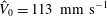 $\hat{V}_{0}=113~\text{mm}~\text{s}^{-1}$
; (f)
$\hat{V}_{0}=113~\text{mm}~\text{s}^{-1}$
; (f)
 $\unicode[STIX]{x1D6FD}=85^{\circ }$
,
$\unicode[STIX]{x1D6FD}=85^{\circ }$
,
 $\hat{V}_{0}=73~\text{mm}~\text{s}^{-1}$
.
$\hat{V}_{0}=73~\text{mm}~\text{s}^{-1}$
.
Figure 7 shows the spatio-temporal diagrams of the cross-sectional-averaged concentration field,
 $\bar{C}_{{\hat{y}}}(\hat{x},\hat{t})$
, for the same experiments as shown in figure 6(b). The green region in the vicinity of
$\bar{C}_{{\hat{y}}}(\hat{x},\hat{t})$
, for the same experiments as shown in figure 6(b). The green region in the vicinity of
 $\hat{x}=0~\text{mm}$
corresponds to the gate valve. It can be seen that there is initially a highly unstable phase present for almost all the flows, manifested through wavy patterns at small
$\hat{x}=0~\text{mm}$
corresponds to the gate valve. It can be seen that there is initially a highly unstable phase present for almost all the flows, manifested through wavy patterns at small
 $\hat{x}$
and
$\hat{x}$
and
 $\hat{t}$
. This phenomenon, which was briefly introduced earlier in figure 2, is similar in nature to that reported by Seon et al. (Reference Seon, Hulin, Salin, Perrin and Hinch2005, Reference Seon, Znaien, Salin, Hulin, Hinch and Perrin2007b
) for exchange flow of miscible fluids, and can be associated with the strong inertial forces balancing buoyancy at the beginning of the displacement flow. At later times, the buoyancy is balanced by viscous forces, reducing the contribution of the inertial forces and relaxing the flow (less steep slopes in the spatio-temporal diagram). The trace of the kinks and droplets forming within the flow due to an interfacial instability is also evident from figure 7(a–e). Another important note here is that the boundary between displacing and displaced fluids remains sharp in the spatio-temporal diagrams for immiscible flows, whereas it can be diffuse for miscible fluids due to mixing and molecular diffusion; see Alba et al. (Reference Alba, Taghavi and Frigaard2013a
) for spatio-temporal diagrams of miscible flows shown in figure 6(a).
$\hat{t}$
. This phenomenon, which was briefly introduced earlier in figure 2, is similar in nature to that reported by Seon et al. (Reference Seon, Hulin, Salin, Perrin and Hinch2005, Reference Seon, Znaien, Salin, Hulin, Hinch and Perrin2007b
) for exchange flow of miscible fluids, and can be associated with the strong inertial forces balancing buoyancy at the beginning of the displacement flow. At later times, the buoyancy is balanced by viscous forces, reducing the contribution of the inertial forces and relaxing the flow (less steep slopes in the spatio-temporal diagram). The trace of the kinks and droplets forming within the flow due to an interfacial instability is also evident from figure 7(a–e). Another important note here is that the boundary between displacing and displaced fluids remains sharp in the spatio-temporal diagrams for immiscible flows, whereas it can be diffuse for miscible fluids due to mixing and molecular diffusion; see Alba et al. (Reference Alba, Taghavi and Frigaard2013a
) for spatio-temporal diagrams of miscible flows shown in figure 6(a).

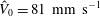
Figure 8. Change in the displacement flow with increasing
 $\hat{V}_{0}$
for the same parameters as shown in figure 6(b) except for
$\hat{V}_{0}$
for the same parameters as shown in figure 6(b) except for
 $\unicode[STIX]{x1D6FD}=45^{\circ }$
and (a)
$\unicode[STIX]{x1D6FD}=45^{\circ }$
and (a)
 $\hat{V}_{0}=0~\text{mm}~\text{s}^{-1}$
(exchange flow), (b)
$\hat{V}_{0}=0~\text{mm}~\text{s}^{-1}$
(exchange flow), (b)
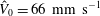 $\hat{V}_{0}=66~\text{mm}~\text{s}^{-1}$
, (c)
$\hat{V}_{0}=66~\text{mm}~\text{s}^{-1}$
, (c)
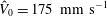 $\hat{V}_{0}=175~\text{mm}~\text{s}^{-1}$
, (d)
$\hat{V}_{0}=175~\text{mm}~\text{s}^{-1}$
, (d)
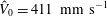 $\hat{V}_{0}=411~\text{mm}~\text{s}^{-1}$
and (e)
$\hat{V}_{0}=411~\text{mm}~\text{s}^{-1}$
and (e)
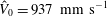 $\hat{V}_{0}=937~\text{mm}~\text{s}^{-1}$
. The snapshots belong to
$\hat{V}_{0}=937~\text{mm}~\text{s}^{-1}$
. The snapshots belong to
 $\hat{t}=10.6,8.8,6.0,2.6,1.3~\text{s}$
, respectively (
$\hat{t}=10.6,8.8,6.0,2.6,1.3~\text{s}$
, respectively (
 $At=0.125$
,
$At=0.125$
,
 $Re\in [0,2196]$
,
$Re\in [0,2196]$
,
 $Fr\in [0,8.67]$
,
$Fr\in [0,8.67]$
,
 $Ca\in [0,\infty ]$
,
$Ca\in [0,\infty ]$
,
 $\unicode[STIX]{x1D703}=56^{\circ }$
). The field of view is
$\unicode[STIX]{x1D703}=56^{\circ }$
). The field of view is
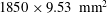 $1850\times 9.53~\text{mm}^{2}$
.
$1850\times 9.53~\text{mm}^{2}$
.
A natural question to ask is that how does the picture given in immiscible displacement flows, e.g. in figure 6(b), change with varying the mean imposed velocity,
 $\hat{V}_{0}$
, or the pumping rate? Figure 8 shows the snapshots of a sequence of immiscible experiments for increasing
$\hat{V}_{0}$
, or the pumping rate? Figure 8 shows the snapshots of a sequence of immiscible experiments for increasing
 $\hat{V}_{0}$
at
$\hat{V}_{0}$
at
 $\unicode[STIX]{x1D6FD}=45^{\circ }$
and
$\unicode[STIX]{x1D6FD}=45^{\circ }$
and
 $At=0.125$
. Figure 8(a) corresponds to
$At=0.125$
. Figure 8(a) corresponds to
 $\hat{V}_{0}=0$
i.e. the exchange configuration. We can interestingly observe that even though the heavy fluid is placed on top of the light one, there is no flow development in this case due to the capillary blockage; see Hulin et al. (Reference Hulin, Znaien, Mendonca, Sourbier, Moisy, Salin and Hinch2008). In the case of miscible fluids there is always a flow as soon as the slightest density difference is applied; see Seon et al. (Reference Seon, Hulin, Salin, Perrin and Hinch2005). Let us have a deeper look into the blockage phenomenon. Examples of the interface shape between heavy and light fluids at various inclination angles in the case of exchange flow and capillary blockage are shown in figure 9. Note that since the gate valve region does not allow us to visualize the interface between the two fluids, we used a different pipe for pictures in figure 9 than the one used in experiments. The pipe properties and diameter are exactly the same as those in our experiments. It can be observed that the interface is curved in a way that the surface tension force can balance that of gravity. The interface curvature is slightly different at various inclination angles. For instance, as the pipe is inclined towards the horizontal direction, the domed-shaped interface is elastically deformed such that the heavy and light fluids accumulate mainly close to the lower and upper parts of the pipe respectively (slumping).
$\hat{V}_{0}=0$
i.e. the exchange configuration. We can interestingly observe that even though the heavy fluid is placed on top of the light one, there is no flow development in this case due to the capillary blockage; see Hulin et al. (Reference Hulin, Znaien, Mendonca, Sourbier, Moisy, Salin and Hinch2008). In the case of miscible fluids there is always a flow as soon as the slightest density difference is applied; see Seon et al. (Reference Seon, Hulin, Salin, Perrin and Hinch2005). Let us have a deeper look into the blockage phenomenon. Examples of the interface shape between heavy and light fluids at various inclination angles in the case of exchange flow and capillary blockage are shown in figure 9. Note that since the gate valve region does not allow us to visualize the interface between the two fluids, we used a different pipe for pictures in figure 9 than the one used in experiments. The pipe properties and diameter are exactly the same as those in our experiments. It can be observed that the interface is curved in a way that the surface tension force can balance that of gravity. The interface curvature is slightly different at various inclination angles. For instance, as the pipe is inclined towards the horizontal direction, the domed-shaped interface is elastically deformed such that the heavy and light fluids accumulate mainly close to the lower and upper parts of the pipe respectively (slumping).
Assuming a simple vertical pipe filled with two immiscible fluids (heavy on top of light), the decay/growth of an interfacial perturbation in the form of Rayleigh–Taylor instability would dictate blockage/non-blockage patterns. The Rayleigh–Taylor instability originating from the presence of a heavy fluid on top of a light one has extensively been investigated in the literature; see Boffetta & Mazzino (Reference Boffetta and Mazzino2017) for the most recent review. In the absence of a surface tension, i.e. miscible fluids, the flow is always unstable as expansively reported by Seon et al. (Reference Seon, Hulin, Salin, Perrin and Hinch2004, Reference Seon, Hulin, Salin, Perrin and Hinch2005, Reference Seon, Hulin, Salin, Perrin and Hinch2006, Reference Seon, Znaien, Salin, Hulin, Hinch and Perrin2007a
). However, for immiscible fluids there exists a critical perturbation wavelength,
 $\hat{\unicode[STIX]{x1D706}}_{cr}$
, below which the flow can be stable. Through linear stability analysis, such a wavelength is given as the following; see Liu et al. (Reference Liu, George, Bo and Glimm2006)
$\hat{\unicode[STIX]{x1D706}}_{cr}$
, below which the flow can be stable. Through linear stability analysis, such a wavelength is given as the following; see Liu et al. (Reference Liu, George, Bo and Glimm2006)
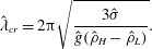 $$\begin{eqnarray}\hat{\unicode[STIX]{x1D706}}_{cr}=2\unicode[STIX]{x03C0}\sqrt{\frac{3\hat{\unicode[STIX]{x1D70E}}}{{\hat{g}}(\hat{\unicode[STIX]{x1D70C}}_{H}-\hat{\unicode[STIX]{x1D70C}}_{L})}}.\end{eqnarray}$$
Using the parameters of a typical capillary blockage case (
 $\hat{\unicode[STIX]{x1D70C}}_{H}=1067~\text{kg}~\text{m}^{-3}$
,
$\hat{\unicode[STIX]{x1D70C}}_{H}=1067~\text{kg}~\text{m}^{-3}$
,
 $\hat{\unicode[STIX]{x1D70C}}_{L}=918~\text{kg}~\text{m}^{-3}$
and
$\hat{\unicode[STIX]{x1D70C}}_{L}=918~\text{kg}~\text{m}^{-3}$
and
 $\hat{\unicode[STIX]{x1D70E}}=3.5~\text{mN}~\text{m}^{-1}$
), the critical wavelength is obtained as
$\hat{\unicode[STIX]{x1D70E}}=3.5~\text{mN}~\text{m}^{-1}$
), the critical wavelength is obtained as
 $\hat{\unicode[STIX]{x1D706}}_{cr}\approx 16.84~\text{mm}$
which is larger than the radius of our pipe (
$\hat{\unicode[STIX]{x1D706}}_{cr}\approx 16.84~\text{mm}$
which is larger than the radius of our pipe (
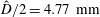 $\hat{D}/2=4.77~\text{mm}$
). Thus the flow is theoretically predicted to be stable which is also confirmed experimentally (figure 9).
$\hat{D}/2=4.77~\text{mm}$
). Thus the flow is theoretically predicted to be stable which is also confirmed experimentally (figure 9).

Figure 9. Examples of formation of capillary blockage between heavy salt water (
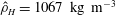 $\hat{\unicode[STIX]{x1D70C}}_{H}=1067~\text{kg}~\text{m}^{-3}$
) and light silicone oil (
$\hat{\unicode[STIX]{x1D70C}}_{H}=1067~\text{kg}~\text{m}^{-3}$
) and light silicone oil (
 $\hat{\unicode[STIX]{x1D70C}}_{L}=918~\text{kg}~\text{m}^{-3}$
) solutions at various inclination angles (
$\hat{\unicode[STIX]{x1D70C}}_{L}=918~\text{kg}~\text{m}^{-3}$
) solutions at various inclination angles (
 $\hat{\unicode[STIX]{x1D70E}}=3.5~\text{mN}~\text{m}^{-1}$
). The red dotted lines are guide to the eye showing domed and slumping-type interface shapes as the pipe is inclined towards the horizontal direction.
$\hat{\unicode[STIX]{x1D70E}}=3.5~\text{mN}~\text{m}^{-1}$
). The red dotted lines are guide to the eye showing domed and slumping-type interface shapes as the pipe is inclined towards the horizontal direction.
As the mean imposed velocity increases (figure 8
b–e), the flow develops through overcoming the capillary blockage. It can be seen from figure 8 that the inertia has shortened the wavelength of the instabilities at the interface between the two fluids; compare figure 8(b) to 8(c–e). Given the limited length of the pipe used in our experiments, it is not clear how the wavelength of the interfacial instabilities in high flow rate cases (figure 8(c–e)) will change over time and distance. Further increasing the mean flow speed breaks down the approximate two-layered slumping structure of the flow (figure 8
b–c) resulting in the dispersed flows (figure 8
e). The dispersed flows are characterized by the droplets that advance through the pipe centreline surrounded by the bulk fluid. The Reynolds number of the imposed flow in several of our experiments, such as the one in figure 8(e), can be marginally larger than the laminar–turbulent transition threshold (
 $Re\approx 2100$
). This can potentially cause (weak) intermittent turbulence in the flow, in turn, enhancing local mixing and droplet formation. The effect of
$Re\approx 2100$
). This can potentially cause (weak) intermittent turbulence in the flow, in turn, enhancing local mixing and droplet formation. The effect of
 $\hat{V}_{0}$
on the flow discussed here persists over other inclination angles and density differences (results not presented for brevity).
$\hat{V}_{0}$
on the flow discussed here persists over other inclination angles and density differences (results not presented for brevity).
3.2 Front velocity measurement
Taghavi et al. (Reference Taghavi, Seon, Martinez and Frigaard2009) found that at long times, the ratio of the mean flow speed to the displacing front velocity,
 $\hat{V}_{0}/\hat{V}_{f}$
, approximates the volume fraction of the light fluid behind the front that is displaced i.e. displacement efficiency. Consequently, it becomes important to measure
$\hat{V}_{0}/\hat{V}_{f}$
, approximates the volume fraction of the light fluid behind the front that is displaced i.e. displacement efficiency. Consequently, it becomes important to measure
 $\hat{V}_{f}$
in a consistent and repeatable way. The front velocity can be measured via tracking the cross-sectional-averaged concentration profile,
$\hat{V}_{f}$
in a consistent and repeatable way. The front velocity can be measured via tracking the cross-sectional-averaged concentration profile,
 $\bar{C}_{{\hat{y}}}$
, over time. Figure 10(a) depicts the evolution of
$\bar{C}_{{\hat{y}}}$
, over time. Figure 10(a) depicts the evolution of
 $\bar{C}_{{\hat{y}}}$
along the pipe,
$\bar{C}_{{\hat{y}}}$
along the pipe,
 $\hat{x}$
, at different times
$\hat{x}$
, at different times
 $\hat{t}=[0.083,1.33,2.583,\ldots ,8.83]~\text{s}$
, for a typical experiment shown in figure 1(b). To avoid noise in the data close to the lower wall of the pipe, we estimate the speed of the displacement front by the velocity of the concentration level
$\hat{t}=[0.083,1.33,2.583,\ldots ,8.83]~\text{s}$
, for a typical experiment shown in figure 1(b). To avoid noise in the data close to the lower wall of the pipe, we estimate the speed of the displacement front by the velocity of the concentration level
 $\bar{C}_{{\hat{y}}}=0.05$
(see the solid line in figure 10
a). One can similarly measure the speed of the trailing front,
$\bar{C}_{{\hat{y}}}=0.05$
(see the solid line in figure 10
a). One can similarly measure the speed of the trailing front,
 $\hat{V}_{tf}$
, by tracking a concentration level close to
$\hat{V}_{tf}$
, by tracking a concentration level close to
 $1$
. Due to slight noise close to this limit,
$1$
. Due to slight noise close to this limit,
 $\bar{C}_{{\hat{y}}}=0.9$
value has been selected as the threshold, marked by dashed line in figure 10(a).
$\bar{C}_{{\hat{y}}}=0.9$
value has been selected as the threshold, marked by dashed line in figure 10(a).

Figure 10. (a) Evolution of the cross-sectional-averaged concentration field,
 $\bar{C}_{{\hat{y}}}(\hat{x},\hat{t})$
, with time,
$\bar{C}_{{\hat{y}}}(\hat{x},\hat{t})$
, with time,
 $\hat{t}=[0.083,1.33,2.583,\ldots ,8.83]~\text{s}$
, and streamwise location,
$\hat{t}=[0.083,1.33,2.583,\ldots ,8.83]~\text{s}$
, and streamwise location,
 $\hat{x}$
, measured from the gate valve for the same experiment as in figure 1(b). The red solid line shows
$\hat{x}$
, measured from the gate valve for the same experiment as in figure 1(b). The red solid line shows
 $\bar{C}_{{\hat{y}}}=0.05$
which is used as threshold for measuring the displacing front velocity,
$\bar{C}_{{\hat{y}}}=0.05$
which is used as threshold for measuring the displacing front velocity,
 $\hat{V}_{f}$
, consistently. The black dashed line shows
$\hat{V}_{f}$
, consistently. The black dashed line shows
 $\bar{C}_{{\hat{y}}}=0.9$
used as threshold in measuring the trailing front velocity,
$\bar{C}_{{\hat{y}}}=0.9$
used as threshold in measuring the trailing front velocity,
 $\hat{V}_{tf}$
. (b) Evolution of the displacing and trailing front velocity values,
$\hat{V}_{tf}$
. (b) Evolution of the displacing and trailing front velocity values,
 $\hat{V}_{f}$
and
$\hat{V}_{f}$
and
 $\hat{V}_{tf}$
, with time for the same experiment.
$\hat{V}_{tf}$
, with time for the same experiment.
Figure 10(b) shows the variation of the displacing and trailing front velocities,
 $\hat{V}_{f}$
and
$\hat{V}_{f}$
and
 $\hat{V}_{tf}$
respectively, with time, which is quite typical in most of our experiments. After opening the gate valve at
$\hat{V}_{tf}$
respectively, with time, which is quite typical in most of our experiments. After opening the gate valve at
 $\hat{t}=0$
, the velocities abruptly increase from
$\hat{t}=0$
, the velocities abruptly increase from
 $0$
(stationary flow) but relax back to steady levels, at longer times (
$0$
(stationary flow) but relax back to steady levels, at longer times (
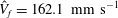 $\hat{V}_{f}=162.1~\text{mm}~\text{s}^{-1}$
and
$\hat{V}_{f}=162.1~\text{mm}~\text{s}^{-1}$
and
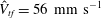 $\hat{V}_{tf}=56~\text{mm}~\text{s}^{-1}$
for the case depicted with approximately
$\hat{V}_{tf}=56~\text{mm}~\text{s}^{-1}$
for the case depicted with approximately
 $1.7\,\%$
and
$1.7\,\%$
and
 $7.2\,\%$
standard deviation respectively). See also Cantero et al. (Reference Cantero, Lee, Balachandar and Garcia2007) for analogous behaviour witnessed in gravity currents. Representative of industrial applications, we are interested in long-time phenomena far from initial transients such as in figure 2. The displacing front velocity seems to be consistently larger than that of the trailing front, suggesting constant stretching of the interface; see also figure 1(b). The selection of a threshold value is a trade-off between robustness and proximity to
$7.2\,\%$
standard deviation respectively). See also Cantero et al. (Reference Cantero, Lee, Balachandar and Garcia2007) for analogous behaviour witnessed in gravity currents. Representative of industrial applications, we are interested in long-time phenomena far from initial transients such as in figure 2. The displacing front velocity seems to be consistently larger than that of the trailing front, suggesting constant stretching of the interface; see also figure 1(b). The selection of a threshold value is a trade-off between robustness and proximity to
 $\bar{C}_{{\hat{y}}}=0,1$
. In order to ensure the validity of the technique, the
$\bar{C}_{{\hat{y}}}=0,1$
. In order to ensure the validity of the technique, the
 $\hat{V}_{f}$
and
$\hat{V}_{f}$
and
 $\hat{V}_{tf}$
readings have also been compared with another method based on the slope of the displacing and displaced fluid edges in the spatio-temporal diagram. Values of
$\hat{V}_{tf}$
readings have also been compared with another method based on the slope of the displacing and displaced fluid edges in the spatio-temporal diagram. Values of
 $\hat{V}_{f}=158.3~\text{mm}~\text{s}^{-1}$
and
$\hat{V}_{f}=158.3~\text{mm}~\text{s}^{-1}$
and
 $\hat{V}_{tf}=51~\text{mm}~\text{s}^{-1}$
(with standard deviations
$\hat{V}_{tf}=51~\text{mm}~\text{s}^{-1}$
(with standard deviations
 $2.2\,\%$
and
$2.2\,\%$
and
 $2.7\,\%$
) have correspondingly been obtained showing close agreement with the threshold method. Note that while the varying length of light path in the transverse
$2.7\,\%$
) have correspondingly been obtained showing close agreement with the threshold method. Note that while the varying length of light path in the transverse
 $\hat{z}$
direction with depth of the pipe can slightly impact
$\hat{z}$
direction with depth of the pipe can slightly impact
 $C$
and
$C$
and
 $\bar{C}_{{\hat{y}}}$
, it does not affect
$\bar{C}_{{\hat{y}}}$
, it does not affect
 $\hat{V}_{f}$
and
$\hat{V}_{f}$
and
 $\hat{V}_{tf}$
measurement.
$\hat{V}_{tf}$
measurement.
We now explore the main characteristics of front velocity measurements across our experimental range, where we have varied inclination angles,
 $\unicode[STIX]{x1D6FD}$
, mean flow speeds
$\unicode[STIX]{x1D6FD}$
, mean flow speeds
 $\hat{V}_{0}$
and density differences,
$\hat{V}_{0}$
and density differences,
 $At$
. Note that in terms of process design, the displacing front,
$At$
. Note that in terms of process design, the displacing front,
 $\hat{V}_{f}$
is of more importance than the trailing one,
$\hat{V}_{f}$
is of more importance than the trailing one,
 $\hat{V}_{tf}$
. We thus focus mostly on the former throughout the rest of the paper. Figure 11(a,b) shows
$\hat{V}_{tf}$
. We thus focus mostly on the former throughout the rest of the paper. Figure 11(a,b) shows
 $\hat{V}_{f}$
for experiments conducted with
$\hat{V}_{f}$
for experiments conducted with
 $At=0.075$
and
$At=0.075$
and
 $0.125$
respectively. In each experimental sequence, at fixed
$0.125$
respectively. In each experimental sequence, at fixed
 $At$
and
$At$
and
 $\unicode[STIX]{x1D6FD}$
, the experiment is carried out at successively higher
$\unicode[STIX]{x1D6FD}$
, the experiment is carried out at successively higher
 $\hat{V}_{0}$
, starting from exchange flow (
$\hat{V}_{0}$
, starting from exchange flow (
 $\hat{V}_{0}=0$
). The values of the front velocity naturally increase with the mean flow speed,
$\hat{V}_{0}=0$
). The values of the front velocity naturally increase with the mean flow speed,
 $\hat{V}_{0}$
. While
$\hat{V}_{0}$
. While
 $\hat{V}_{f}$
strongly changes with
$\hat{V}_{f}$
strongly changes with
 $\hat{V}_{0}$
, it weakly depends on the inclination angle,
$\hat{V}_{0}$
, it weakly depends on the inclination angle,
 $\unicode[STIX]{x1D6FD}$
, and Atwood number,
$\unicode[STIX]{x1D6FD}$
, and Atwood number,
 $At$
.
$At$
.
Figure 11. Change in displacing front velocity,
 $\hat{V}_{f}$
, with tilt angle,
$\hat{V}_{f}$
, with tilt angle,
 $\unicode[STIX]{x1D6FD}$
, and imposed flow velocity,
$\unicode[STIX]{x1D6FD}$
, and imposed flow velocity,
 $\hat{V}_{0}$
, for (a)
$\hat{V}_{0}$
, for (a)
 $At=0.075$
and (b)
$At=0.075$
and (b)
 $At=0.125$
. Different markers represent
$At=0.125$
. Different markers represent
 $\hat{V}_{0}=0$
(
$\hat{V}_{0}=0$
(
 $\times$
for capillary blockage and ▹ for exchange flow),
$\times$
for capillary blockage and ▹ for exchange flow),
 $50$
(▪),
$50$
(▪),
 $100$
(♦),
$100$
(♦),
 $300$
(◂),
$300$
(◂),
 $500$
(▴),
$500$
(▴),
 $700$
(*),
$700$
(*),
 $900$
(○) and
$900$
(○) and
 $1100~\text{mm}~\text{s}^{-1}$
(▾). The dashed lines are guide to the eye plotted at
$1100~\text{mm}~\text{s}^{-1}$
(▾). The dashed lines are guide to the eye plotted at
 $\hat{V}_{f}=50,100,200,\ldots ,1200,1300~\text{mm}~\text{s}^{-1}$
.
$\hat{V}_{f}=50,100,200,\ldots ,1200,1300~\text{mm}~\text{s}^{-1}$
.

Figure 12. Presentation of our results for the full range of experiments for
 $At=0.075$
and
$At=0.075$
and
 $0.125$
(
$0.125$
(
 $\unicode[STIX]{x1D703}=56^{\circ }$
): normalized front velocity
$\unicode[STIX]{x1D703}=56^{\circ }$
): normalized front velocity
 $\hat{V}_{f}/\hat{V}_{0}$
, plotted against
$\hat{V}_{f}/\hat{V}_{0}$
, plotted against
 $Re$
and
$Re$
and
 $Re\cos \unicode[STIX]{x1D6FD}/Fr$
. For
$Re\cos \unicode[STIX]{x1D6FD}/Fr$
. For
 $0\leqslant Re\lesssim 730$
indicated by a dashed line, we have
$0\leqslant Re\lesssim 730$
indicated by a dashed line, we have
 $V_{f}>1.5$
. Normalized front velocity scale is limited to
$V_{f}>1.5$
. Normalized front velocity scale is limited to
 $1.5$
to better show the variations of the front velocity in the plane of
$1.5$
to better show the variations of the front velocity in the plane of
 $Re$
and
$Re$
and
 $Re\cos \unicode[STIX]{x1D6FD}/Fr$
. All the displacement flows in the range given were found to be in the instantaneous regime.
$Re\cos \unicode[STIX]{x1D6FD}/Fr$
. All the displacement flows in the range given were found to be in the instantaneous regime.
Let us now proceed with a dimensionless analysis of the results, focusing on the normalized front velocity,
 $V_{f}=\hat{V}_{f}/\hat{V}_{0}$
. In our previous study of miscible displacements, see Taghavi et al. (Reference Taghavi, Alba, Seon, Wielage-Burchard, Martinez and Frigaard2012b
) and Alba et al. (Reference Alba, Taghavi and Frigaard2013a
), we were able to classify all the flows in
$V_{f}=\hat{V}_{f}/\hat{V}_{0}$
. In our previous study of miscible displacements, see Taghavi et al. (Reference Taghavi, Alba, Seon, Wielage-Burchard, Martinez and Frigaard2012b
) and Alba et al. (Reference Alba, Taghavi and Frigaard2013a
), we were able to classify all the flows in
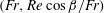 $(Fr,Re\cos \unicode[STIX]{x1D6FD}/Fr)$
plane. Note that
$(Fr,Re\cos \unicode[STIX]{x1D6FD}/Fr)$
plane. Note that
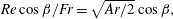 $$\begin{eqnarray}Re\cos \unicode[STIX]{x1D6FD}/Fr=\sqrt{Ar/2}\cos \unicode[STIX]{x1D6FD},\end{eqnarray}$$
where
 $$\begin{eqnarray}Ar=(\hat{\unicode[STIX]{x1D70C}}_{H}+\hat{\unicode[STIX]{x1D70C}}_{L})(\hat{\unicode[STIX]{x1D70C}}_{H}-\hat{\unicode[STIX]{x1D70C}}_{L}){\hat{g}}\hat{D}^{3}/(2\hat{\unicode[STIX]{x1D707}}^{2}),\end{eqnarray}$$
is the Archimedes number. The parameter
 $Re\cos \unicode[STIX]{x1D6FD}/Fr$
is independent of
$Re\cos \unicode[STIX]{x1D6FD}/Fr$
is independent of
 $\hat{V}_{0}$
and represents the relative strengths of buoyancy stresses
$\hat{V}_{0}$
and represents the relative strengths of buoyancy stresses
 $(\hat{\unicode[STIX]{x1D70C}}_{H}-\hat{\unicode[STIX]{x1D70C}}_{L}){\hat{g}}\hat{D}\cos \unicode[STIX]{x1D6FD}$
, to viscous stresses,
$(\hat{\unicode[STIX]{x1D70C}}_{H}-\hat{\unicode[STIX]{x1D70C}}_{L}){\hat{g}}\hat{D}\cos \unicode[STIX]{x1D6FD}$
, to viscous stresses,
 $\hat{\unicode[STIX]{x1D707}}\hat{V}_{t}/\hat{D}$
. We start with this description except we aim to classify the flows in
$\hat{\unicode[STIX]{x1D707}}\hat{V}_{t}/\hat{D}$
. We start with this description except we aim to classify the flows in
 $(Re,Re\cos \unicode[STIX]{x1D6FD}/Fr)$
instead, in order to conveniently be able to relate to the mean imposed flow strength in terms of process design. Figure 12 shows the normalized front velocity,
$(Re,Re\cos \unicode[STIX]{x1D6FD}/Fr)$
instead, in order to conveniently be able to relate to the mean imposed flow strength in terms of process design. Figure 12 shows the normalized front velocity,
 $V_{f}=\hat{V}_{f}/\hat{V}_{0}$
, plotted against
$V_{f}=\hat{V}_{f}/\hat{V}_{0}$
, plotted against
 $Re$
and
$Re$
and
 $Re\cos \unicode[STIX]{x1D6FD}/Fr$
, for all experiments conducted in this study for
$Re\cos \unicode[STIX]{x1D6FD}/Fr$
, for all experiments conducted in this study for
 $At=0.075$
and
$At=0.075$
and
 $0.125$
. The exchange flow data have not been included due to their singularity (
$0.125$
. The exchange flow data have not been included due to their singularity (
 $\hat{V}_{0}=0$
). Our first observation is that over nearly the entire range of
$\hat{V}_{0}=0$
). Our first observation is that over nearly the entire range of
 $Re\cos \unicode[STIX]{x1D6FD}/Fr$
studied,
$Re\cos \unicode[STIX]{x1D6FD}/Fr$
studied,
 $V_{f}$
increases as
$V_{f}$
increases as
 $Re$
decreases. As
$Re$
decreases. As
 $Re\rightarrow 0$
, we approach the exchange flow limit. For
$Re\rightarrow 0$
, we approach the exchange flow limit. For
 $Re\lesssim 730$
we observe a number of flows for which
$Re\lesssim 730$
we observe a number of flows for which
 $V_{f}>1.5$
(highlighted by a dashed line). Note that the scale in figure 12 is adjusted such that to emphasize the experiments for which
$V_{f}>1.5$
(highlighted by a dashed line). Note that the scale in figure 12 is adjusted such that to emphasize the experiments for which
 $V_{f}>1.5$
. The actual data vary in the range
$V_{f}>1.5$
. The actual data vary in the range
 $1<V_{f}<2.7$
. In the case of miscible flows we have
$1<V_{f}<2.7$
. In the case of miscible flows we have
 $1<V_{f}<3.3$
, see Alba et al. (Reference Alba, Taghavi and Frigaard2013a
), emphasizing that
$1<V_{f}<3.3$
, see Alba et al. (Reference Alba, Taghavi and Frigaard2013a
), emphasizing that
 $\hat{V}_{f}$
in the immiscible flows is closer to
$\hat{V}_{f}$
in the immiscible flows is closer to
 $\hat{V}_{0}$
i.e. more efficient displacement. All the displacement flows in the range given were found to be in the instantaneous regime (no back flow). The picture given in figure 12 may, in general, vary with the Atwood number, however, we did not find a noticeable change for the range
$\hat{V}_{0}$
i.e. more efficient displacement. All the displacement flows in the range given were found to be in the instantaneous regime (no back flow). The picture given in figure 12 may, in general, vary with the Atwood number, however, we did not find a noticeable change for the range
 $At\in [0.075{-}0.125]$
. In order to assess the robustness of the choice of controlling parameters of the problem, it is useful to test flow regime classification i.e. fast (
$At\in [0.075{-}0.125]$
. In order to assess the robustness of the choice of controlling parameters of the problem, it is useful to test flow regime classification i.e. fast (
 $V_{f}>1.5$
) versus slow (
$V_{f}>1.5$
) versus slow (
 $1<V_{f}<1.5$
) experiments, in a map other than
$1<V_{f}<1.5$
) experiments, in a map other than
 $Re\cos \unicode[STIX]{x1D6FD}/Fr-Re$
. In particular, we are interested to see how the classification unfolds by the surface tension parameter i.e. capillary number,
$Re\cos \unicode[STIX]{x1D6FD}/Fr-Re$
. In particular, we are interested to see how the classification unfolds by the surface tension parameter i.e. capillary number,
 $Ca$
. It is found that, in the plane of
$Ca$
. It is found that, in the plane of
 $Re\cos \unicode[STIX]{x1D6FD}/Fr-Ca$
, the flows with
$Re\cos \unicode[STIX]{x1D6FD}/Fr-Ca$
, the flows with
 $V_{f}>1.5$
locate in the low range of the capillary number,
$V_{f}>1.5$
locate in the low range of the capillary number,
 $Ca\leqslant 0.5$
(results not presented here for brevity). As
$Ca\leqslant 0.5$
(results not presented here for brevity). As
 $Ca$
is increased (enhancement of viscous stress relative to surface tension due to flow acceleration), the dimensionless front velocity relaxes to lower values (
$Ca$
is increased (enhancement of viscous stress relative to surface tension due to flow acceleration), the dimensionless front velocity relaxes to lower values (
 $\hat{V}_{f}$
becomes closer to
$\hat{V}_{f}$
becomes closer to
 $\hat{V}_{0}$
).
$\hat{V}_{0}$
).
Figure 13(a) shows snapshots of the flow for CaCl
 $_{2}$
–water displacing silicone oil suggesting a simple (rather stable) layered pattern. In order to analyse the immiscible flow velocity field we may define four flow zones namely B, C, D and E. Zone B characterizes Poiseuille flow of a single fluid (oil) which is indeed captured in figure 13(b) via UDV measurements. Reflection effects at the lower wall of the pipe make it difficult to measure a zero velocity at the lower wall; see also Taghavi et al. (Reference Taghavi, Alba, Seon, Wielage-Burchard, Martinez and Frigaard2012b
), Alba et al. (Reference Alba, Taghavi and Frigaard2013a
) for similar effects. The dotted lines in figure 13(b–e) are guides to the eye correcting for this artefact. In zone C, the pipe is partly filled with displacing and displaced fluids. Figure 13(c) depicts the velocity profile recorded over this period. The interface height measured from our visualization has also been added to the figure for comparison. The figure shows a bulged region within the displacing fluid (velocity maximum just below the interface) dragging the displaced layer downstream due to viscous stress. Measuring the velocity profile using UDV for immiscible systems can be extremely difficult, especially when the interface is moving as discussed recently by Amini, De Cesare & Schleiss (Reference Amini, De Cesare and Schleiss2009). The fluids immiscibility causes refraction errors in the vicinity of the interface which in turn can affect the neighbouring acoustic field. This erroneous region has been identified by dashed lines in figure 13(c,d).
$_{2}$
–water displacing silicone oil suggesting a simple (rather stable) layered pattern. In order to analyse the immiscible flow velocity field we may define four flow zones namely B, C, D and E. Zone B characterizes Poiseuille flow of a single fluid (oil) which is indeed captured in figure 13(b) via UDV measurements. Reflection effects at the lower wall of the pipe make it difficult to measure a zero velocity at the lower wall; see also Taghavi et al. (Reference Taghavi, Alba, Seon, Wielage-Burchard, Martinez and Frigaard2012b
), Alba et al. (Reference Alba, Taghavi and Frigaard2013a
) for similar effects. The dotted lines in figure 13(b–e) are guides to the eye correcting for this artefact. In zone C, the pipe is partly filled with displacing and displaced fluids. Figure 13(c) depicts the velocity profile recorded over this period. The interface height measured from our visualization has also been added to the figure for comparison. The figure shows a bulged region within the displacing fluid (velocity maximum just below the interface) dragging the displaced layer downstream due to viscous stress. Measuring the velocity profile using UDV for immiscible systems can be extremely difficult, especially when the interface is moving as discussed recently by Amini, De Cesare & Schleiss (Reference Amini, De Cesare and Schleiss2009). The fluids immiscibility causes refraction errors in the vicinity of the interface which in turn can affect the neighbouring acoustic field. This erroneous region has been identified by dashed lines in figure 13(c,d).

Figure 13. (a) Experimental snapshots for
 $\unicode[STIX]{x1D6FD}=85^{\circ }$
,
$\unicode[STIX]{x1D6FD}=85^{\circ }$
,
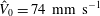 $\hat{V}_{0}=74~\text{mm}~\text{s}^{-1}$
,
$\hat{V}_{0}=74~\text{mm}~\text{s}^{-1}$
,
 $\hat{\unicode[STIX]{x1D70C}}_{H}=1181~\text{kg}~\text{m}^{-3}$
and
$\hat{\unicode[STIX]{x1D70C}}_{H}=1181~\text{kg}~\text{m}^{-3}$
and
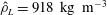 $\hat{\unicode[STIX]{x1D70C}}_{L}=918~\text{kg}~\text{m}^{-3}$
at times
$\hat{\unicode[STIX]{x1D70C}}_{L}=918~\text{kg}~\text{m}^{-3}$
at times
 $\hat{t}=[0.250,1.725,3.200,\ldots ,7.625]~\text{s}$
, with a field of view
$\hat{t}=[0.250,1.725,3.200,\ldots ,7.625]~\text{s}$
, with a field of view
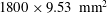 $1800\times 9.53~\text{mm}^{2}$
(
$1800\times 9.53~\text{mm}^{2}$
(
 $At=0.125$
,
$At=0.125$
,
 $Re=148$
,
$Re=148$
,
 $Fr=0.69$
,
$Fr=0.69$
,
 $Ca=0.11$
,
$Ca=0.11$
,
 $\unicode[STIX]{x1D703}=56^{\circ }$
). The bottommost image is a colour bar of concentration
$\unicode[STIX]{x1D703}=56^{\circ }$
). The bottommost image is a colour bar of concentration
 $C$
, with
$C$
, with
 $0$
and
$0$
and
 $1$
referring to the displaced and displacing fluids respectively. Each snapshot is assigned a letter B to E. The representative UDV profiles to these flows are plotted in panels (b–e). (b) Velocity profile averaged over
$1$
referring to the displaced and displacing fluids respectively. Each snapshot is assigned a letter B to E. The representative UDV profiles to these flows are plotted in panels (b–e). (b) Velocity profile averaged over
 $\hat{t}=[0,3.00]~\text{s}$
, when only the displaced oil flows under the UDV probe. (c) Velocity profile averaged over
$\hat{t}=[0,3.00]~\text{s}$
, when only the displaced oil flows under the UDV probe. (c) Velocity profile averaged over
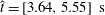 $\hat{t}=[3.64,5.55]~\text{s}$
, when there is a stratification of oil and water layers. The horizontal blue dash-dotted line shows the interface height. The dashed line highlights the region affected by the error due to a moving oil–water interface. (d) Velocity profile at
$\hat{t}=[3.64,5.55]~\text{s}$
, when there is a stratification of oil and water layers. The horizontal blue dash-dotted line shows the interface height. The dashed line highlights the region affected by the error due to a moving oil–water interface. (d) Velocity profile at
 $\hat{t}\approx 5.69~\text{s}$
, capturing slip-type behaviour at the upper wall. Similar to panel (c), the dashed line highlights the erroneous region affected by an immiscible oil–water interface. (e) Velocity profile averaged over
$\hat{t}\approx 5.69~\text{s}$
, capturing slip-type behaviour at the upper wall. Similar to panel (c), the dashed line highlights the erroneous region affected by an immiscible oil–water interface. (e) Velocity profile averaged over
 $\hat{t}=[5.85,7.20]~\text{s}$
, when only the displacing water-based solution flows under the UDV probe. The dotted lines in panels (b–e) for
$\hat{t}=[5.85,7.20]~\text{s}$
, when only the displacing water-based solution flows under the UDV probe. The dotted lines in panels (b–e) for
 ${\hat{y}}\lesssim 1~\text{mm}$
, are guides to the eye correcting the UDV refraction errors close to the lower wall.
${\hat{y}}\lesssim 1~\text{mm}$
, are guides to the eye correcting the UDV refraction errors close to the lower wall.
The displacing and displaced fluids in the vicinity of the pipe walls (
 ${\hat{y}}=0,\hat{D}$
) introduce a contact line problem which is well known to be mathematically singular if one is to assume conventional no-slip condition; see for instance Dussan (Reference Dussan1979). A concrete argument in explaining the contact problem has been proposed by Greenspan (Reference Greenspan1978), Spaid & Homsy (Reference Spaid and Homsy1996) through introducing a Navier-slip, rather than no-slip, condition at the wall. A great application of UDV in our experiments can be in detecting the slip-type behaviour of the flow close to the contact line. For this purpose, we carefully examined our experiments finding the exact time at which the contact line passes the UDV location. Figure 13(d) depicts the velocity profile at this time (zone D in figure 13
a). Upon comparison with the rest of the UDV profiles e.g. in zones B and C, we can identify a sharp slip-type increase in the velocity close to the upper wall of the pipe. Similar behaviour persists in other experiments. Note that akin slip-type patterns close to the contact line have been reported in the computational study of Redapangu et al. (Reference Redapangu, Sahu and Vanka2012a
) carried out for displacement flow of immiscible fluids at comparable range of the Reynolds number. We believe that the slip-type behaviour at the wall has a major effect in increasing the displacement efficiency in the case of immiscible fluids compared to the miscible ones; see figure 6. Figure 13(e) shows the typical velocity field for zone E where the pipe is fully occupied by the displacing fluid, again supporting a Poiseuille-type profile. Finally, note that we are unable to analyse the velocity profile of the flows exhibiting strong Kelvin–Helmholtz and Rayleigh instabilities due to the inherent high level of noise present in the UDV data of such cases.
${\hat{y}}=0,\hat{D}$
) introduce a contact line problem which is well known to be mathematically singular if one is to assume conventional no-slip condition; see for instance Dussan (Reference Dussan1979). A concrete argument in explaining the contact problem has been proposed by Greenspan (Reference Greenspan1978), Spaid & Homsy (Reference Spaid and Homsy1996) through introducing a Navier-slip, rather than no-slip, condition at the wall. A great application of UDV in our experiments can be in detecting the slip-type behaviour of the flow close to the contact line. For this purpose, we carefully examined our experiments finding the exact time at which the contact line passes the UDV location. Figure 13(d) depicts the velocity profile at this time (zone D in figure 13
a). Upon comparison with the rest of the UDV profiles e.g. in zones B and C, we can identify a sharp slip-type increase in the velocity close to the upper wall of the pipe. Similar behaviour persists in other experiments. Note that akin slip-type patterns close to the contact line have been reported in the computational study of Redapangu et al. (Reference Redapangu, Sahu and Vanka2012a
) carried out for displacement flow of immiscible fluids at comparable range of the Reynolds number. We believe that the slip-type behaviour at the wall has a major effect in increasing the displacement efficiency in the case of immiscible fluids compared to the miscible ones; see figure 6. Figure 13(e) shows the typical velocity field for zone E where the pipe is fully occupied by the displacing fluid, again supporting a Poiseuille-type profile. Finally, note that we are unable to analyse the velocity profile of the flows exhibiting strong Kelvin–Helmholtz and Rayleigh instabilities due to the inherent high level of noise present in the UDV data of such cases.

Figure 14. Static contact angles obtained for salt-water/oil solutions used in our study in the same acrylic pipe as used for the experiments: (a) silicone oil (
 $\hat{\unicode[STIX]{x1D70C}}=918~\text{kg}~\text{m}^{-3}$
,
$\hat{\unicode[STIX]{x1D70C}}=918~\text{kg}~\text{m}^{-3}$
,
 $\hat{\unicode[STIX]{x1D707}}=0.005~\text{Pa}~\text{s}$
,
$\hat{\unicode[STIX]{x1D707}}=0.005~\text{Pa}~\text{s}$
,
 $\hat{\unicode[STIX]{x1D70E}}=3.5~\text{mN}~\text{m}^{-1}$
), (b) light viscosity mineral oil (
$\hat{\unicode[STIX]{x1D70E}}=3.5~\text{mN}~\text{m}^{-1}$
), (b) light viscosity mineral oil (
 $\hat{\unicode[STIX]{x1D70C}}=853~\text{kg}~\text{m}^{-3}$
,
$\hat{\unicode[STIX]{x1D70C}}=853~\text{kg}~\text{m}^{-3}$
,
 $\hat{\unicode[STIX]{x1D707}}=0.014~\text{Pa}~\text{s}$
,
$\hat{\unicode[STIX]{x1D707}}=0.014~\text{Pa}~\text{s}$
,
 $\hat{\unicode[STIX]{x1D70E}}=10.1~\text{mN}~\text{m}^{-1}$
) and (c) heavy viscosity mineral oil (
$\hat{\unicode[STIX]{x1D70E}}=10.1~\text{mN}~\text{m}^{-1}$
) and (c) heavy viscosity mineral oil (
 $\hat{\unicode[STIX]{x1D70C}}=864~\text{kg}~\text{m}^{-3}$
,
$\hat{\unicode[STIX]{x1D70C}}=864~\text{kg}~\text{m}^{-3}$
,
 $\hat{\unicode[STIX]{x1D707}}=0.084~\text{Pa}~\text{s}$
,
$\hat{\unicode[STIX]{x1D707}}=0.084~\text{Pa}~\text{s}$
,
 $\hat{\unicode[STIX]{x1D70E}}=33.4~\text{mN}~\text{m}^{-1}$
). The vertical red lines indicate inner pipe wall positions. Note that for the sets shown
$\hat{\unicode[STIX]{x1D70E}}=33.4~\text{mN}~\text{m}^{-1}$
). The vertical red lines indicate inner pipe wall positions. Note that for the sets shown
 $At=0.125$
.
$At=0.125$
.

Figure 15. Snapshots of experiments for immiscible displacement flows for
 $At=0.125$
. (a) Salt-water displacing silicone oil with
$At=0.125$
. (a) Salt-water displacing silicone oil with
 $\hat{\unicode[STIX]{x1D70C}}_{H}=1181~\text{kg}~\text{m}^{-3}$
,
$\hat{\unicode[STIX]{x1D70C}}_{H}=1181~\text{kg}~\text{m}^{-3}$
,
 $\hat{\unicode[STIX]{x1D70C}}_{L}=918~\text{kg}~\text{m}^{-3}$
,
$\hat{\unicode[STIX]{x1D70C}}_{L}=918~\text{kg}~\text{m}^{-3}$
,
 $\hat{\unicode[STIX]{x1D707}}=0.005~\text{Pa}~\text{s}$
,
$\hat{\unicode[STIX]{x1D707}}=0.005~\text{Pa}~\text{s}$
,
 $\hat{\unicode[STIX]{x1D70E}}=3.5~\text{mN}~\text{m}^{-1}$
and
$\hat{\unicode[STIX]{x1D70E}}=3.5~\text{mN}~\text{m}^{-1}$
and
 $\unicode[STIX]{x1D703}=56^{\circ }$
(
$\unicode[STIX]{x1D703}=56^{\circ }$
(
 $Re\in [141,315]$
,
$Re\in [141,315]$
,
 $Fr\in [0.60,1.19]$
,
$Fr\in [0.60,1.19]$
,
 $Ca\in [0.04,0.34]$
). From left to right
$Ca\in [0.04,0.34]$
). From left to right
 $\hat{V}_{0}=81,73,159~\text{mm}~\text{s}^{-1}$
, and
$\hat{V}_{0}=81,73,159~\text{mm}~\text{s}^{-1}$
, and
 $\hat{t}=8.5,8.5,7~\text{s}$
. (b) Salt-water displacing light viscosity mineral oil with
$\hat{t}=8.5,8.5,7~\text{s}$
. (b) Salt-water displacing light viscosity mineral oil with
 $\hat{\unicode[STIX]{x1D70C}}_{H}=1097~\text{kg}~\text{m}^{-3}$
,
$\hat{\unicode[STIX]{x1D70C}}_{H}=1097~\text{kg}~\text{m}^{-3}$
,
 $\hat{\unicode[STIX]{x1D70C}}_{L}=853~\text{kg}~\text{m}^{-3}$
,
$\hat{\unicode[STIX]{x1D70C}}_{L}=853~\text{kg}~\text{m}^{-3}$
,
 $\hat{\unicode[STIX]{x1D707}}=0.014~\text{Pa}~\text{s}$
,
$\hat{\unicode[STIX]{x1D707}}=0.014~\text{Pa}~\text{s}$
,
 $\hat{\unicode[STIX]{x1D70E}}=10.1~\text{mN}~\text{m}^{-1}$
and
$\hat{\unicode[STIX]{x1D70E}}=10.1~\text{mN}~\text{m}^{-1}$
and
 $\unicode[STIX]{x1D703}=52^{\circ }$
(
$\unicode[STIX]{x1D703}=52^{\circ }$
(
 $Re\in [45,145]$
,
$Re\in [45,145]$
,
 $Fr\in [0.46,1.46]$
,
$Fr\in [0.46,1.46]$
,
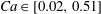 $Ca\in [0.02,0.51]$
). From left to right
$Ca\in [0.02,0.51]$
). From left to right
 $\hat{V}_{0}=62,84,196~\text{mm}~\text{s}^{-1}$
, and
$\hat{V}_{0}=62,84,196~\text{mm}~\text{s}^{-1}$
, and
 $\hat{t}=10,10,5.4~\text{s}$
. (c) Salt-water displacing heavy viscosity mineral oil with
$\hat{t}=10,10,5.4~\text{s}$
. (c) Salt-water displacing heavy viscosity mineral oil with
 $\hat{\unicode[STIX]{x1D70C}}_{H}=1110~\text{kg}~\text{m}^{-3}$
,
$\hat{\unicode[STIX]{x1D70C}}_{H}=1110~\text{kg}~\text{m}^{-3}$
,
 $\hat{\unicode[STIX]{x1D70C}}_{L}=864~\text{kg}~\text{m}^{-3}$
,
$\hat{\unicode[STIX]{x1D70C}}_{L}=864~\text{kg}~\text{m}^{-3}$
,
 $\hat{\unicode[STIX]{x1D707}}=0.084~\text{Pa}~\text{s}$
,
$\hat{\unicode[STIX]{x1D707}}=0.084~\text{Pa}~\text{s}$
,
 $\hat{\unicode[STIX]{x1D70E}}=33.4~\text{mN}~\text{m}^{-1}$
and
$\hat{\unicode[STIX]{x1D70E}}=33.4~\text{mN}~\text{m}^{-1}$
and
 $\unicode[STIX]{x1D703}=59^{\circ }$
(
$\unicode[STIX]{x1D703}=59^{\circ }$
(
 $Re\in [7,20]$
,
$Re\in [7,20]$
,
 $Fr\in [0.46,1.10]$
,
$Fr\in [0.46,1.10]$
,
 $Ca\in [0.03,0.57]$
). From left to right
$Ca\in [0.03,0.57]$
). From left to right
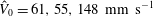 $\hat{V}_{0}=61,55,148~\text{mm}~\text{s}^{-1}$
, and
$\hat{V}_{0}=61,55,148~\text{mm}~\text{s}^{-1}$
, and
 $\hat{t}=14,14,7.5~\text{s}$
. The field of view for all the figures shown is
$\hat{t}=14,14,7.5~\text{s}$
. The field of view for all the figures shown is
 $1550\times 9.53~\text{mm}^{2}$
located just below the gate valve.
$1550\times 9.53~\text{mm}^{2}$
located just below the gate valve.
3.3 Other water–oil solutions
It is useful at this stage to verify whether the general flow patterns reported above for immiscible flows hold for various fluid pairs other than the salt water and silicone oil. To address this, two other displaced fluid oils were used namely light viscosity and heavy viscosity mineral oils. Figure 14 shows slight variation in static contact angles obtained for various oils used. A high-resolution DSLR Canon100D with macro lens was used to obtain the images as the resolution is the key in determining fluids contact angles. In particular, we followed the methodology of Lamour et al. (Reference Lamour, Hamraoui, Buvailo, Xing, Keuleyan, Prakash, Eftekhari-Bafrooei and Borguet2010) in analysing the images employing ImageJ software contact angle plugin. The error in reading was found to be
 $\pm 1.5^{\circ }$
.
$\pm 1.5^{\circ }$
.
Figure 15(a–c) shows immiscible displacement flows over a range of inclination angles and imposed velocities for salt water displacing silicone oil and light and heavy viscosity mineral oils respectively for
 $At=0.125$
. The mean imposed velocities,
$At=0.125$
. The mean imposed velocities,
 $\hat{V}_{0}$
, and time snapshots,
$\hat{V}_{0}$
, and time snapshots,
 $\hat{t}$
, in different figures are chosen closely to make a direct comparison between the figures feasible. Also note that the displacing fluid solutions were viscosified accordingly using xanthan gum (
$\hat{t}$
, in different figures are chosen closely to make a direct comparison between the figures feasible. Also note that the displacing fluid solutions were viscosified accordingly using xanthan gum (
 $245,450,1170~\text{mg}~\text{L}^{-1}$
for silicone oil and light and heavy viscosity mineral oils respectively) to ensure an iso-viscous study. The shear-thinning effects for higher concentration of xanthan become important, however, not in the range of shear rates considered in our experiments. The flow patterns observed between various types of oil appear to be similar overall. Note that the wettability and interfacial tension in the ranges considered do not affect slip-type effects, i.e. the displaced fluids still seem to have been successfully removed resulting in high displacement efficiencies. The two-layered slumping patterns are found at inclination angles
$245,450,1170~\text{mg}~\text{L}^{-1}$
for silicone oil and light and heavy viscosity mineral oils respectively) to ensure an iso-viscous study. The shear-thinning effects for higher concentration of xanthan become important, however, not in the range of shear rates considered in our experiments. The flow patterns observed between various types of oil appear to be similar overall. Note that the wettability and interfacial tension in the ranges considered do not affect slip-type effects, i.e. the displaced fluids still seem to have been successfully removed resulting in high displacement efficiencies. The two-layered slumping patterns are found at inclination angles
 $\unicode[STIX]{x1D6FD}=30^{\circ },60^{\circ }$
. At vertical configuration (
$\unicode[STIX]{x1D6FD}=30^{\circ },60^{\circ }$
. At vertical configuration (
 $\unicode[STIX]{x1D6FD}=0^{\circ }$
), the displacing fluid instead advances mostly in the central region of the pipe.
$\unicode[STIX]{x1D6FD}=0^{\circ }$
), the displacing fluid instead advances mostly in the central region of the pipe.

Figure 16. Snapshots of experiments for immiscible exchange/displacement flows for
 $\hat{\unicode[STIX]{x1D70C}}_{H}=1355~\text{kg}~\text{m}^{-3}$
and
$\hat{\unicode[STIX]{x1D70C}}_{H}=1355~\text{kg}~\text{m}^{-3}$
and
 $\hat{\unicode[STIX]{x1D70C}}_{L}=918~\text{kg}~\text{m}^{-3}$
(
$\hat{\unicode[STIX]{x1D70C}}_{L}=918~\text{kg}~\text{m}^{-3}$
(
 $At=0.192$
and
$At=0.192$
and
 $\unicode[STIX]{x1D703}=56^{\circ }$
). (a) From left to right
$\unicode[STIX]{x1D703}=56^{\circ }$
). (a) From left to right
 $\hat{V}_{0}=0~\text{mm}~\text{s}^{-1}$
,
$\hat{V}_{0}=0~\text{mm}~\text{s}^{-1}$
,
 $\hat{t}=[33.1,11.9,25]~\text{s}$
(
$\hat{t}=[33.1,11.9,25]~\text{s}$
(
 $Re=0$
,
$Re=0$
,
 $Fr=\infty$
,
$Fr=\infty$
,
 $Ca=\infty$
). Note that at
$Ca=\infty$
). Note that at
 $\unicode[STIX]{x1D6FD}=0^{\circ }$
there occurs capillary blockage. (b) From left to right
$\unicode[STIX]{x1D6FD}=0^{\circ }$
there occurs capillary blockage. (b) From left to right
 $\hat{V}_{0}=[10,47,14]~\text{mm}~\text{s}^{-1}$
,
$\hat{V}_{0}=[10,47,14]~\text{mm}~\text{s}^{-1}$
,
 $\hat{t}=[31.8,8.8,12.5]~\text{s}$
(
$\hat{t}=[31.8,8.8,12.5]~\text{s}$
(
 $Re=[21,102,30]$
,
$Re=[21,102,30]$
,
 $Fr=[0.07,0.35,0.10]$
). The position of the displacing front in
$Fr=[0.07,0.35,0.10]$
). The position of the displacing front in
 $\unicode[STIX]{x1D6FD}=0^{\circ }$
case is marked by an arrow. (c) From left to right
$\unicode[STIX]{x1D6FD}=0^{\circ }$
case is marked by an arrow. (c) From left to right
 $\hat{V}_{0}=[15,53,59]~\text{mm}~\text{s}^{-1}$
,
$\hat{V}_{0}=[15,53,59]~\text{mm}~\text{s}^{-1}$
,
 $\hat{t}=[30.9,7.8,6.75]~\text{s}$
(
$\hat{t}=[30.9,7.8,6.75]~\text{s}$
(
 $Re=[33,114,128]$
,
$Re=[33,114,128]$
,
 $Fr=[0.11,0.39,0.44]$
). The field of view in all the snapshots is
$Fr=[0.11,0.39,0.44]$
). The field of view in all the snapshots is
 $1650\times 9.53~\text{mm}^{2}$
.
$1650\times 9.53~\text{mm}^{2}$
.
3.4 Trailing front behaviour
In the limit of miscible fluids, Taghavi et al. (Reference Taghavi, Alba, Seon, Wielage-Burchard, Martinez and Frigaard2012b
) identified the behaviour of the trailing front as sustained back flow, stationary interface, temporary back flow and instantaneous displacement. Briefly, for strong buoyancy compared to the mean flow strength, the displaced layer may continue travelling upstream (sustained back flow). As the mean flow speed,
 $\hat{V}_{0}$
, is increased, the displaced layer travels upstream but stops at a location above the gate valve (stationary interface). The flow within the displaced layer in this case is only recirculated by pumping the displacing layer. At progressively higher mean flow speeds, the back flow forms temporarily but then disappears over time (temporary back flow) or eventually may not form at all (instantaneous displacement). We are interested to know how this picture changes in the case of immiscible fluids. Figure 16 shows snapshots of experiments for
$\hat{V}_{0}$
, is increased, the displaced layer travels upstream but stops at a location above the gate valve (stationary interface). The flow within the displaced layer in this case is only recirculated by pumping the displacing layer. At progressively higher mean flow speeds, the back flow forms temporarily but then disappears over time (temporary back flow) or eventually may not form at all (instantaneous displacement). We are interested to know how this picture changes in the case of immiscible fluids. Figure 16 shows snapshots of experiments for
 $At=0.192$
at different angles and carefully increasing values of the mean flow speed from (a–c). Note that we had to add significant amount of salt to the aqueous solutions (close to the saturation limit) to observe any back flow in our immiscible experiments. There exists a continuous back flow at
$At=0.192$
at different angles and carefully increasing values of the mean flow speed from (a–c). Note that we had to add significant amount of salt to the aqueous solutions (close to the saturation limit) to observe any back flow in our immiscible experiments. There exists a continuous back flow at
 $\hat{V}_{0}=0$
except for
$\hat{V}_{0}=0$
except for
 $\unicode[STIX]{x1D6FD}=0^{\circ }$
where a capillary blockage occurs (figure 16
a). As
$\unicode[STIX]{x1D6FD}=0^{\circ }$
where a capillary blockage occurs (figure 16
a). As
 $\hat{V}_{0}$
is increased in figure 16(b), the displaced layer stops at the gate valve location which can be similar to the stationary interface case for miscible flows. Eventually, we observe movement of the trailing front at higher
$\hat{V}_{0}$
is increased in figure 16(b), the displaced layer stops at the gate valve location which can be similar to the stationary interface case for miscible flows. Eventually, we observe movement of the trailing front at higher
 $\hat{V}_{0}$
as evident from figure 16(c). In summary, it appears as though only three regimes namely sustained back flow, stationary interface and instantaneous displacement exist in the case of immiscible fluids as opposed to the four regimes of the miscible limit. Note that studying non-Boussinesq flows beyond the Atwood number considered (
$\hat{V}_{0}$
as evident from figure 16(c). In summary, it appears as though only three regimes namely sustained back flow, stationary interface and instantaneous displacement exist in the case of immiscible fluids as opposed to the four regimes of the miscible limit. Note that studying non-Boussinesq flows beyond the Atwood number considered (
 $At=0.192$
) is not possible in our experiments due to the limitations in the density of salt as well as its solubility in water.
$At=0.192$
) is not possible in our experiments due to the limitations in the density of salt as well as its solubility in water.

Figure 17. Presentation of our data in the exchange limit (
 $\hat{V}_{0}=Re=Fr=0$
) in the
$\hat{V}_{0}=Re=Fr=0$
) in the
 $(Fr/Ca,\sqrt{Ar/2}\cos \unicode[STIX]{x1D6FD})$
plane identifying capillary blockage/non-blockage regimes.
$(Fr/Ca,\sqrt{Ar/2}\cos \unicode[STIX]{x1D6FD})$
plane identifying capillary blockage/non-blockage regimes.
3.5 Regime classification
We now aim to classify various flow regime types observed between two immiscible fluids in dimensionless maps. Let us first consider the simple case of exchange flow where the mean imposed velocity is zero (
 $\hat{V}_{0}=Re=Fr=0$
). In §§ 3.1 and 3.4 we learnt that depending on the inclination angle and the strength of capillary to buoyancy force, either blockage or non-blockage flows may emerge. The exchange flow data over our range of experiments have been plotted in figure 17 in the plane of
$\hat{V}_{0}=Re=Fr=0$
). In §§ 3.1 and 3.4 we learnt that depending on the inclination angle and the strength of capillary to buoyancy force, either blockage or non-blockage flows may emerge. The exchange flow data over our range of experiments have been plotted in figure 17 in the plane of
 $(Fr/Ca,\sqrt{Ar/2}\cos \unicode[STIX]{x1D6FD})$
. Note that
$(Fr/Ca,\sqrt{Ar/2}\cos \unicode[STIX]{x1D6FD})$
. Note that
 $Fr$
and
$Fr$
and
 $Ca$
, individually, would be zero for all exchange data since
$Ca$
, individually, would be zero for all exchange data since
 $\hat{V}_{0}=0$
but the ratio
$\hat{V}_{0}=0$
but the ratio
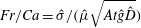 $Fr/Ca=\hat{\unicode[STIX]{x1D70E}}/(\hat{\unicode[STIX]{x1D707}}\sqrt{At{\hat{g}}\hat{D}})$
resolves such singularity. From (3.4) we further realized that
$Fr/Ca=\hat{\unicode[STIX]{x1D70E}}/(\hat{\unicode[STIX]{x1D707}}\sqrt{At{\hat{g}}\hat{D}})$
resolves such singularity. From (3.4) we further realized that
 $\sqrt{Ar/2}\cos \unicode[STIX]{x1D6FD}(=Re\cos \unicode[STIX]{x1D6FD}/Fr)$
captures buoyant-to-viscous stress. As
$\sqrt{Ar/2}\cos \unicode[STIX]{x1D6FD}(=Re\cos \unicode[STIX]{x1D6FD}/Fr)$
captures buoyant-to-viscous stress. As
 $Fr/Ca\rightarrow 0$
(
$Fr/Ca\rightarrow 0$
(
 $\hat{\unicode[STIX]{x1D70E}}\rightarrow 0$
) we can spot the appearance of more non-blockage flows (weakened capillary force). On the other hand, as
$\hat{\unicode[STIX]{x1D70E}}\rightarrow 0$
) we can spot the appearance of more non-blockage flows (weakened capillary force). On the other hand, as
 $Fr/Ca\rightarrow \infty$
(
$Fr/Ca\rightarrow \infty$
(
 $\hat{\unicode[STIX]{x1D70E}}\rightarrow \infty$
) we increasingly observe blockage flows which is in agreement with finding of relation (3.3) presented earlier.
$\hat{\unicode[STIX]{x1D70E}}\rightarrow \infty$
) we increasingly observe blockage flows which is in agreement with finding of relation (3.3) presented earlier.

Figure 18. Classification of our results presented in the
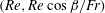 $(Re,Re\cos \unicode[STIX]{x1D6FD}/Fr)$
-plane: (i) viscous flows marked by red circles; (ii) transitionary flows marked with blue triangles; and (iii) dispersed flows marked with green squares. Note that the picture given is primarily obtained for
$(Re,Re\cos \unicode[STIX]{x1D6FD}/Fr)$
-plane: (i) viscous flows marked by red circles; (ii) transitionary flows marked with blue triangles; and (iii) dispersed flows marked with green squares. Note that the picture given is primarily obtained for
 $At\in [0.075,0.125]$
and the contact angle
$At\in [0.075,0.125]$
and the contact angle
 $\unicode[STIX]{x1D703}=56^{\circ }$
. The dashed lines correspond to
$\unicode[STIX]{x1D703}=56^{\circ }$
. The dashed lines correspond to
 $Re\cos \unicode[STIX]{x1D6FD}/Fr=50$
,
$Re\cos \unicode[STIX]{x1D6FD}/Fr=50$
,
 $Re=730$
and
$Re=730$
and
 $Re=1000$
. The snapshots are obtained for viscous:
$Re=1000$
. The snapshots are obtained for viscous:
 $\unicode[STIX]{x1D6FD}=85^{\circ }$
,
$\unicode[STIX]{x1D6FD}=85^{\circ }$
,
 $\unicode[STIX]{x1D70C}_{H}=1181~\text{kg}~\text{m}^{-3}$
,
$\unicode[STIX]{x1D70C}_{H}=1181~\text{kg}~\text{m}^{-3}$
,
 $\unicode[STIX]{x1D70C}_{L}=918~\text{kg}~\text{m}^{-3}$
,
$\unicode[STIX]{x1D70C}_{L}=918~\text{kg}~\text{m}^{-3}$
,
 $\hat{V}_{0}=74~\text{mm}~\text{s}^{-1}$
at
$\hat{V}_{0}=74~\text{mm}~\text{s}^{-1}$
at
 $\hat{t}=7.6~\text{s}$
(
$\hat{t}=7.6~\text{s}$
(
 $At=0.125$
,
$At=0.125$
,
 $Re=148$
,
$Re=148$
,
 $Fr=0.68$
,
$Fr=0.68$
,
 $Ca=0.10$
), transitionary:
$Ca=0.10$
), transitionary:
 $\unicode[STIX]{x1D6FD}=15^{\circ }$
,
$\unicode[STIX]{x1D6FD}=15^{\circ }$
,
 $\unicode[STIX]{x1D70C}_{H}=1067~\text{kg}~\text{m}^{-3}$
,
$\unicode[STIX]{x1D70C}_{H}=1067~\text{kg}~\text{m}^{-3}$
,
 $\unicode[STIX]{x1D70C}_{L}=918~\text{kg}~\text{m}^{-3}$
,
$\unicode[STIX]{x1D70C}_{L}=918~\text{kg}~\text{m}^{-3}$
,
 $\hat{V}_{0}=73~\text{mm}~\text{s}^{-1}$
at
$\hat{V}_{0}=73~\text{mm}~\text{s}^{-1}$
at
 $\hat{t}=14.2~\text{s}$
(
$\hat{t}=14.2~\text{s}$
(
 $At=0.075$
,
$At=0.075$
,
 $Re=130$
,
$Re=130$
,
 $Fr=0.87$
,
$Fr=0.87$
,
 $Ca=0.11$
) and dispersed flows:
$Ca=0.11$
) and dispersed flows:
 $\unicode[STIX]{x1D6FD}=45^{\circ }$
,
$\unicode[STIX]{x1D6FD}=45^{\circ }$
,
 $\unicode[STIX]{x1D70C}_{H}=1067~\text{kg}~\text{m}^{-3}$
,
$\unicode[STIX]{x1D70C}_{H}=1067~\text{kg}~\text{m}^{-3}$
,
 $\unicode[STIX]{x1D70C}_{L}=918~\text{kg}~\text{m}^{-3}$
,
$\unicode[STIX]{x1D70C}_{L}=918~\text{kg}~\text{m}^{-3}$
,
 $\hat{V}_{0}=874~\text{mm}~\text{s}^{-1}$
at
$\hat{V}_{0}=874~\text{mm}~\text{s}^{-1}$
at
 $\hat{t}=1.8~\text{s}$
(
$\hat{t}=1.8~\text{s}$
(
 $At=0.075$
,
$At=0.075$
,
 $Re=1652$
,
$Re=1652$
,
 $Fr=10.44$
,
$Fr=10.44$
,
 $Ca=1.25$
). The field of view in the snapshots shown is
$Ca=1.25$
). The field of view in the snapshots shown is
 $1800\times 9.53~\text{mm}^{2}$
.
$1800\times 9.53~\text{mm}^{2}$
.
Upon closely looking into the immiscible displacement flow experiments, and in comparison with the miscible limit, three major regimes may be identified along with the classification given in (
 $Re-Re\cos \unicode[STIX]{x1D6FD}/Fr$
)-plane. (i) Viscous flows: similar to the miscible limit, there were found a number of immiscible flows where the degree of instability is low i.e. the fluids stay stratified with minimal interfacial wave formation; see e.g.
$Re-Re\cos \unicode[STIX]{x1D6FD}/Fr$
)-plane. (i) Viscous flows: similar to the miscible limit, there were found a number of immiscible flows where the degree of instability is low i.e. the fluids stay stratified with minimal interfacial wave formation; see e.g.
 $\unicode[STIX]{x1D6FD}=85^{\circ }$
in figures 6(b) and 13. These flows were found to mainly occur in a rectangular region bounded by
$\unicode[STIX]{x1D6FD}=85^{\circ }$
in figures 6(b) and 13. These flows were found to mainly occur in a rectangular region bounded by
 $Re\approx 1000$
and
$Re\approx 1000$
and
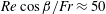 $Re\cos \unicode[STIX]{x1D6FD}/Fr\approx 50$
and are marked by red circles in figure 18. (ii) Transitionary flows: the flow instability in these flows is enhanced up to a point they result in evident interfacial waves and/or droplet formation, see e.g.
$Re\cos \unicode[STIX]{x1D6FD}/Fr\approx 50$
and are marked by red circles in figure 18. (ii) Transitionary flows: the flow instability in these flows is enhanced up to a point they result in evident interfacial waves and/or droplet formation, see e.g.
 $\unicode[STIX]{x1D6FD}=30^{\circ },45^{\circ },60^{\circ },75^{\circ }$
in figure 6(b). Although droplets may form in this regime due to pearling, the overall structure of the flow is still layered i.e. the heavy displacing fluid slumps beneath the light displaced one. These flows, marked by blue triangles in figure 18, appear for
$\unicode[STIX]{x1D6FD}=30^{\circ },45^{\circ },60^{\circ },75^{\circ }$
in figure 6(b). Although droplets may form in this regime due to pearling, the overall structure of the flow is still layered i.e. the heavy displacing fluid slumps beneath the light displaced one. These flows, marked by blue triangles in figure 18, appear for
 $Re\cos \unicode[STIX]{x1D6FD}/Fr\gtrsim 50$
and
$Re\cos \unicode[STIX]{x1D6FD}/Fr\gtrsim 50$
and
 $Re\lesssim 730$
. Based on figure 12,
$Re\lesssim 730$
. Based on figure 12,
 $Re\lesssim 730$
was also found to be the boundary for the flows with
$Re\lesssim 730$
was also found to be the boundary for the flows with
 $V_{f}>1.5$
. (iii) Dispersed flows: similar to the transitionary flows, the dispersed flows (e.g.
$V_{f}>1.5$
. (iii) Dispersed flows: similar to the transitionary flows, the dispersed flows (e.g.
 $\unicode[STIX]{x1D6FD}=0^{\circ }$
in figures 6
b and 8
e) exhibit a large degree of flow instability. However, the significant difference is that in the latter, the droplets of the displaced fluid move within the centre of the pipe rather than leaning towards the upper and lower walls of the pipe. Another fundamental difference is that in the dispersed flows, both water-in-oil (w/o) and oil-in-water (o/w) dispersions may exist; see closely the dispersed flow snapshot in figure 18 for the droplets forming on the right- and left-hand sides of the pipe respectively. However, in transitionary flows, only o/w dispersion may be found. For similar w/o and o/w classification of immiscible flows see Schümann et al. (Reference Schümann, Tutkun, Yang and Nydal2016). We suspect that for dispersed flows, smaller-sized droplets may form at progressively higher values of
$\unicode[STIX]{x1D6FD}=0^{\circ }$
in figures 6
b and 8
e) exhibit a large degree of flow instability. However, the significant difference is that in the latter, the droplets of the displaced fluid move within the centre of the pipe rather than leaning towards the upper and lower walls of the pipe. Another fundamental difference is that in the dispersed flows, both water-in-oil (w/o) and oil-in-water (o/w) dispersions may exist; see closely the dispersed flow snapshot in figure 18 for the droplets forming on the right- and left-hand sides of the pipe respectively. However, in transitionary flows, only o/w dispersion may be found. For similar w/o and o/w classification of immiscible flows see Schümann et al. (Reference Schümann, Tutkun, Yang and Nydal2016). We suspect that for dispersed flows, smaller-sized droplets may form at progressively higher values of
 $Re$
as also noted in the study of Habchi et al. (Reference Habchi, Lemenand, Della Valle and Peerhossaini2009). The dispersed flows which are marked by green squares in figure 18 emerge for
$Re$
as also noted in the study of Habchi et al. (Reference Habchi, Lemenand, Della Valle and Peerhossaini2009). The dispersed flows which are marked by green squares in figure 18 emerge for
 $Re\gtrsim 1000$
for
$Re\gtrsim 1000$
for
 $Re\cos \unicode[STIX]{x1D6FD}/Fr\lesssim 50$
and
$Re\cos \unicode[STIX]{x1D6FD}/Fr\lesssim 50$
and
 $Re\gtrsim 730$
for
$Re\gtrsim 730$
for
 $Re\cos \unicode[STIX]{x1D6FD}/Fr\gtrsim 50$
. Typical snapshots of representative flows explained here have been added to figure 18 for convenience. Lastly, it is emphasized that the picture provided in this figure is valid for the range
$Re\cos \unicode[STIX]{x1D6FD}/Fr\gtrsim 50$
. Typical snapshots of representative flows explained here have been added to figure 18 for convenience. Lastly, it is emphasized that the picture provided in this figure is valid for the range
 $At\in [0.075,0.125]$
and a configuration where the wetting displacing fluid removes a non-wetting displaced one with contact angle
$At\in [0.075,0.125]$
and a configuration where the wetting displacing fluid removes a non-wetting displaced one with contact angle
 $\unicode[STIX]{x1D703}\approx 56^{\circ }$
. Similar to figure 12, the general features of the phase diagram and flow classification given in figure 18 remain the same if capillary number,
$\unicode[STIX]{x1D703}\approx 56^{\circ }$
. Similar to figure 12, the general features of the phase diagram and flow classification given in figure 18 remain the same if capillary number,
 $Ca$
, is to be chosen instead of
$Ca$
, is to be chosen instead of
 $Re$
in the
$Re$
in the
 $x$
-axis. Results are not shown here for brevity but shortly, the viscous flows locate in a rectangular region bounded between
$x$
-axis. Results are not shown here for brevity but shortly, the viscous flows locate in a rectangular region bounded between
 $0\leqslant Re\cos \unicode[STIX]{x1D6FD}/Fr\leqslant 50$
and
$0\leqslant Re\cos \unicode[STIX]{x1D6FD}/Fr\leqslant 50$
and
 $0\leqslant Ca\leqslant 0.7$
, the transitionary flows in the region
$0\leqslant Ca\leqslant 0.7$
, the transitionary flows in the region
 $Re\cos \unicode[STIX]{x1D6FD}/Fr>50$
and
$Re\cos \unicode[STIX]{x1D6FD}/Fr>50$
and
 $0\leqslant Ca\leqslant 0.5$
and diffusive flows in the rest of
$0\leqslant Ca\leqslant 0.5$
and diffusive flows in the rest of
 $Re\cos \unicode[STIX]{x1D6FD}/Fr-Ca$
plane extending up to
$Re\cos \unicode[STIX]{x1D6FD}/Fr-Ca$
plane extending up to
 $Ca=2$
.
$Ca=2$
.
4 Summary
Displacement flow of two immiscible iso-viscous Newtonian fluids in an inclined pipe have been investigated experimentally in the case where the wetting displacing fluid is denser than the non-wetting displaced fluid (i.e. density unstable). Our experiments have covered a broad range of the governing dimensionless parameter space
 $(\unicode[STIX]{x1D6FD},Re,Fr,Ca,\unicode[STIX]{x1D703})$
, not covered before in any experimental study. Compared to the miscible study of Alba et al. (Reference Alba, Taghavi and Frigaard2013a
), novel flow patterns and instabilities were observed in the immiscible case. The fluids immiscibility is found to significantly increase the displacement efficiency through decreasing the front velocity
$(\unicode[STIX]{x1D6FD},Re,Fr,Ca,\unicode[STIX]{x1D703})$
, not covered before in any experimental study. Compared to the miscible study of Alba et al. (Reference Alba, Taghavi and Frigaard2013a
), novel flow patterns and instabilities were observed in the immiscible case. The fluids immiscibility is found to significantly increase the displacement efficiency through decreasing the front velocity
 $\hat{V}_{f}$
. The displacing layer wets the wall close to the contact line resulting in the removal of the non-wetting displaced fluid. This finding can potentially be very useful in cementing operations where the goal is to remove the in situ displaced fluid meanwhile minimally contaminating the displacing one. The observed effect is persistent over a wide range of oils as the displaced fluid. Ultrasonic Doppler velocimetry has been used to compliment flow visualization, shedding light on the dynamics of the flow and wetting mechanisms at the walls. The early stage of the displacement is found to be governed by strong shearing and Kelvin–Helmholtz instabilities. The intensity of the Kelvin–Helmholtz instabilities is later reduced. Surface-tension-driven Rayleigh-type instabilities, however, remain active in the flow causing droplet shedding (pearling) at displaced fluid receding contact lines. Capillary blockage was found to occur in the absence of the mean imposed flow i.e. exchange configuration, classified in the plane of
$\hat{V}_{f}$
. The displacing layer wets the wall close to the contact line resulting in the removal of the non-wetting displaced fluid. This finding can potentially be very useful in cementing operations where the goal is to remove the in situ displaced fluid meanwhile minimally contaminating the displacing one. The observed effect is persistent over a wide range of oils as the displaced fluid. Ultrasonic Doppler velocimetry has been used to compliment flow visualization, shedding light on the dynamics of the flow and wetting mechanisms at the walls. The early stage of the displacement is found to be governed by strong shearing and Kelvin–Helmholtz instabilities. The intensity of the Kelvin–Helmholtz instabilities is later reduced. Surface-tension-driven Rayleigh-type instabilities, however, remain active in the flow causing droplet shedding (pearling) at displaced fluid receding contact lines. Capillary blockage was found to occur in the absence of the mean imposed flow i.e. exchange configuration, classified in the plane of
 $\sqrt{Ar/2}\cos \unicode[STIX]{x1D6FD}$
and
$\sqrt{Ar/2}\cos \unicode[STIX]{x1D6FD}$
and
 $Fr/Ca$
. We have further classified the displacement flows as viscous, transitionary and dispersed. A qualitative description of each of these flows has been provided, delineating where each flow can be found in the dimensionless planes of
$Fr/Ca$
. We have further classified the displacement flows as viscous, transitionary and dispersed. A qualitative description of each of these flows has been provided, delineating where each flow can be found in the dimensionless planes of
 $Re$
and
$Re$
and
 $Re\cos \unicode[STIX]{x1D6FD}/Fr$
. Lastly, it is emphasized that it would be useful to examine how the flow patterns observed will be affected when the displacing fluid is non-wetting and the displaced one is wetting. However, there are a few limitations to running such experiments as most oils are lighter than water. Due to polarity issues, it is not possible to densify oils using salt to achieve a density-unstable configuration. On the other hand, the density-stable flows are governed through entirely different dynamics than the density-unstable ones (our scope); see for instance Alba, Taghavi & Frigaard (Reference Alba, Taghavi and Frigaard2012), Alba et al. (Reference Alba, Taghavi and Frigaard2013a
) for miscible fluids. Future directions of this work include studying the destabilizing mechanisms of immiscible interfaces theoretically through a weakly inertial weighted-residual model similar to that of Alba, Taghavi & Frigaard (Reference Alba, Taghavi and Frigaard2013b
) developed for miscible fluids. It would also be useful to examine other wetting/non-wetting flow configurations than the one considered in the current work.
$Re\cos \unicode[STIX]{x1D6FD}/Fr$
. Lastly, it is emphasized that it would be useful to examine how the flow patterns observed will be affected when the displacing fluid is non-wetting and the displaced one is wetting. However, there are a few limitations to running such experiments as most oils are lighter than water. Due to polarity issues, it is not possible to densify oils using salt to achieve a density-unstable configuration. On the other hand, the density-stable flows are governed through entirely different dynamics than the density-unstable ones (our scope); see for instance Alba, Taghavi & Frigaard (Reference Alba, Taghavi and Frigaard2012), Alba et al. (Reference Alba, Taghavi and Frigaard2013a
) for miscible fluids. Future directions of this work include studying the destabilizing mechanisms of immiscible interfaces theoretically through a weakly inertial weighted-residual model similar to that of Alba, Taghavi & Frigaard (Reference Alba, Taghavi and Frigaard2013b
) developed for miscible fluids. It would also be useful to examine other wetting/non-wetting flow configurations than the one considered in the current work.
Acknowledgements
This research has been carried out at the University of Houston (UH) through National Research University Fund (NRUF). The authors feel indebted to Professor J. P. Hulin (FAST laboratory, France) for invaluable discussion and guidance forming the foundations of the current study. Helpful comments from Professor I. A. Frigaard (The University of British Columbia, Canada) in improving the presentation of the results are also greatly appreciated. P. Jalalmanesh is sincerely thanked for assisting in running the experiments. A.H. acknowledges the support received from Houston Scholars Program. Finally, the authors thank the reviewers for their extremely useful and constructive comments.


