


1. Introduction
Blending grains with a liquid is an essential step in many industrial processes, for instance in the food industry (Forny, Marabi & Palzer Reference Forny, Marabi and Palzer2011) and in civil engineering for the preparation of building materials (Cazacliu & Roquet Reference Cazacliu and Roquet2009; Collet et al. Reference Collet, Oulahna, De Ryck, Henri and Martin2010). The mixing step often involves initially pouring granular materials into a liquid bath so that the particles are dispersed in the interstitial fluid. At a larger scale, the entry of grains into water occurs during the collapse of a cliff edge at the seaside. In this situation, tsunami waves can be generated by the entry of the granular mass into the ocean, which leads to a significant hazard for the population. This phenomenon has been the subject of experimental work to quantify the amplitude of the waves resulting from these events (Fritz, Hager & Minor Reference Fritz, Hager and Minor2003; Heller, Hager & Minor Reference Heller, Hager and Minor2008; Viroulet, Sauret & Kimmoun Reference Viroulet, Sauret and Kimmoun2014; Robbe-Saule et al. Reference Robbe-Saule, Morize, Henaff, Bertho, Sauret and Gondret2021). Macroscopic theoretical models describing the energy transfer between the grains and the liquid have been proposed to predict the amplitude of the wave generated (Zitti et al. Reference Zitti, Ancey, Postacchini and Brocchini2016; Mulligan & Take Reference Mulligan and Take2017). Nevertheless, an understanding of the interplay between the grains and the liquid is essential for correctly describing the transition from dry to wet grains during the immersion of a dense granular material. This interaction is also important for predicting the liquid and sediment transports in complex granular systems, for instance during the drainage of water from basements after heavy rains (Horton Reference Horton1945; Kirchner, Feng & Neal Reference Kirchner, Feng and Neal2000; Guérin, Devauchelle & Lajeunesse Reference Guérin, Devauchelle and Lajeunesse2014), which also impact the stability of soils subjected to extreme conditions (Herminghaus Reference Herminghaus2005).
The interplay between a granular material and a liquid has been studied in static configurations where the granular material behaves as a porous medium in which the liquid flows. At low Reynolds number, the flow dynamics is captured by Darcy's law, which relates the fluid velocity to the pressure gradient applied to the liquid (Bear Reference Bear1988). For larger Reynolds numbers, inertial effects induce a nonlinear dependence of the pressure gradient on the velocity. Different inertial corrections have been reported in the literature (Bear Reference Bear1988). Among them, Forchheimer's law has successfully been used to capture various situations of flow in porous media (Bear Reference Bear1988). These approaches are used to describe, for instance, capillary flows in porous media in different geometries (Lucas Reference Lucas1918; Washburn Reference Washburn1921; Hyväluoma et al. Reference Hyväluoma, Raiskinmäki, Jäsberg, Koponen, Kataja and Timonen2006; Xiao, Stone & Attinger Reference Xiao, Stone and Attinger2012; Benner & Petsev Reference Benner and Petsev2013), as well as various layered porous systems (Reyssat et al. Reference Reyssat, Sangne, van Nierop and Stone2009; Mensire et al. Reference Mensire, Ault, Lorenceau and Stone2016). Gravity flows in porous media, such as during drainage in aquifers, have also been successfully described using these models (Lyle et al. Reference Lyle, Huppert, Hallworth, Bickle and Chadwick2005; Vella & Huppert Reference Vella and Huppert2006; Guérin et al. Reference Guérin, Devauchelle and Lajeunesse2014). Nevertheless, understanding of the dynamics of a porous medium plunging from the air into a water bath remains elusive.
In this work, we investigate the entry of a dry granular jet in a liquid bath. The granular jet configuration is well-known in the case of impact on a solid surface (Cheng et al. Reference Cheng, Varas, Citron, Jaeger and Nagel2007; Müller, Formella & Pöschel Reference Müller, Formella and Pöschel2014). Conversely, its interaction with a soft or a liquid surface remains a subject of investigation. When the granular material penetrates the liquid bath, it tends to fragment by interacting with the fluid (González Gutiérrez, Carrillo Estrada & Ruiz Suárez Reference González Gutiérrez, Carrillo Estrada and Ruiz Suárez2014; Cervantes-Álvarez et al. Reference Cervantes-Álvarez, Escobar-Ortega, Sauret and Pacheco-Vázquez2020). Once immersed, the flow of grains in an interstitial liquid is governed by the viscous displacement of the particle in the fluid (Courrech du Pont et al. Reference Courrech du Pont, Gondret, Perrin and Rabaud2003; Doppler et al. Reference Doppler, Gondret, Loiseleux, Meyer and Rabaud2007; Topin et al. Reference Topin, Monerie, Perales and Radjaï2012; Bougouin, Lacaze & Bonometti Reference Bougouin, Lacaze and Bonometti2017).
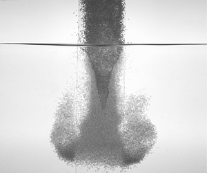
The modelling of a dry granular jet entering water is a complex problem, since the structure of the jet evolves as the grains enter the fluid. Unlike a jet of an immiscible liquid into water, a granular jet impregnates when the particles that compose it are hydrophilic, leading to a complex multiphase situation. Figure 1 shows a time series of a jet of dry grains entering into a quiescent water bath. In the configuration considered here, when the jet crosses the liquid surface, it remains compact and deforms the free surface. As the jet begins to impregnate, there is a dry part located inside the jet (dark grey) surrounded by an impregnated part (light grey). After a short transient, a stationary  $V$-shaped impregnation front appears. The grains only disperse after being entirely wetted by the water. This observation suggests modelling at first order the initial behaviour of a dense granular jet as a porous medium translating into a liquid bath. The situation is reminiscent of the coating processes used to coat textiles or surfaces with a liquid by dragging them into a bath (Quéré Reference Quéré1999; Clarke Reference Clarke2002; Seiwert, Clanet & Quéré Reference Seiwert, Clanet and Quéré2011). When a liquid slides on partially wetting substrates, a
  $V$ shape can also be observed behind a droplet (Podgorski, Flesselles & Limat Reference Podgorski, Flesselles and Limat2001) or for forced wetting and dewetting (Blake & Ruschak Reference Blake and Ruschak1979; He & Nagel Reference He and Nagel2019). In these cases, the
  $V$ shape results from the existence of a limiting wetting velocity of the contact line, which can be estimated to be of the order of 5 m s
 $^{-1}$ for water (He & Nagel Reference He and Nagel2019), far beyond our experimental conditions. Moreover, our configuration differs in the complexity of the surface exposed to the liquid: a porous material that can be impregnated by the liquid. Furthermore, in the case of a porous material, the isotropy of the medium does not constrain an orientation of the fluid front, contrary to the case of the hairy surfaces studied recently by Nasto et al. (Reference Nasto, Regli, Brun, Alvarado, Clanet and Hosoi2016).

Figure 1. Time series of a free semi-2D granular jet penetrating into a water bath. Particles are spherical glass beads of diameter  $d_g=1050\pm 250\ \mathrm {\mu }\textrm {m}$. The jet of width 5 cm is confined between two polymethyl methacrylate (PMMA) plates (at the front and the rear). Each picture is separated from the next by 0.25 s. Scale bar is 2 mm.
In this work, we experimentally investigate the impregnation of a porous material translated into a liquid reservoir. The experimental observations are compared to analytical models and numerical results. The experimental set-up is described in § 2. The transient impregnation regime is reported in § 3 and modelled by a one-dimensional (1D) impregnation dynamics. In § 4, we focus on the stationary regime characterized by a stationary impregnation. This stable profile is then partially modelled using Darcy's and Forchheimer's models in § 5. In § 6, a numerical method is developed to model the shape of the impregnation front fully. Finally, a discussion is proposed in § 7 to compare the results obtained with a porous medium to those obtained with a dense granular jet.
2. Experimental methods
2.1. Experimental set-up
The experimental set-up, shown in figure 2(a), consists of a linear motor stage translating a porous material at a constant velocity  $V_0$ into a water reservoir of large dimensions. The porous medium is formed by packing spherical glass beads into a transparent cell of length 40 cm, of variable width
  $W=5$, 10, or 20 cm and of thickness 12 mm, so that the configuration can be considered bidimensional, as shown in figure 2(b). The side and bottom walls of the cell are permeable thanks to a metal wire mesh with openings of 250
  $\mathrm {\mu }$m (visible in figure 2a). The low thickness of the cell allows us to observe the dry and wet grains as dark and light, respectively, using the contrast of absorption of the light emitted by an LED panel placed behind the set-up (figure 2c). It also allows us to track the impregnation front separating the dry and wet regions.

Figure 2. (a) Photo of the porous medium made of grains (system W3). The front and rear are made of PMMA, and the sides and bottom of the cell consist of a metal wire mesh with openings of 250  $\mathrm {\mu }$m. (b) Schematic of the experimental set-up. A vertical linear motor imposes the speed of translation
  $V_0$. (c) Picture of the stationary impregnation front during the translation of the porous medium into the water bath. The system is illuminated by an LED panel placed behind the cell. The light part is fully saturated with water whereas the dark part is dry.
The porous medium is translated vertically into the water bath at a constant speed  $V_0$ varying between 1 mm s
 $^{-1}$ and 150 mm s
 $^{-1}$. The impregnation dynamics is recorded at 30 frames per second (using a Nikon D-7100 with an F30 lens) and then analysed by image processing to extract the shape of the impregnation front and its time-evolution during the experiment.
2.2. Characterization of porous media
Each porous medium was prepared by filling the transparent cell with glass beads. Different systems of grains were used to tune the pore size and the wettability of the porous medium. We performed the experiments with the systems W1, W2, W3, where W stands for ‘wetting’, and the systems N1 and N2, where N stands for ‘non-wetting’ thanks to coated glass beads (Sigmund Lindner). The coating changes the surface properties of the beads by increasing the contact angle with the liquid. The beads are sieved to refine the size distributions, which are summarized in table 1 (see also Appendix A). For each system, the glass beads are cleaned with soap and thoroughly rinsed with de-ionized water to remove any dust on the grains.
Table 1. Physical properties of the grains composing the model porous media.

The contact angle between the grain and the water is measured by trapping a single bead at the surface of a pending drop of liquid (Timounay, Lorenceau & Rouyer Reference Timounay, Lorenceau and Rouyer2015). For each experiment, the granular packing is prepared by following a protocol detailed in Appendix A. Several taps are given to compact the granular packing until it reaches a constant volume fraction of  $\phi \simeq 0.62$. The compacity
  $\phi$ and the porosity
  $\epsilon$ of the granular packing are estimated by measuring the mass and the volume occupied by the grains (see Appendix A). The permeability is measured by an experiment of filtration through the porous medium, following the procedure presented by Chopin & Kudrolli (Reference Chopin and Kudrolli2011). This measurement is performed at low Reynolds number, in the range of velocities compatible with Darcy's law. The measured permeability is denoted by
  $k_1$ in table 1. Another set of measurements of the permeability is performed at larger Reynolds numbers to determine the Forchheimer coefficient
  $\beta _2$, which is required in the Darcy–Forchheimer equation used in § 5. Furthermore, a third value for the permeability, denoted by
  $k$, is used to fit the theoretical prediction to the experimental data. Only the values
  $k$ and
  $\beta _2$ are used in this paper. The discrepancies between the measurements of the permeability are relatively small and remain less than
  $20\,\%$ for all experimental configurations. The small difference can be explained by experimental artifacts introduced by the glass tube used for the flow measurements through the packed beads. The physical characteristics of all model porous media used in this study are summarized in table 1, and all the experimental methods used to characterize the properties of the beads are detailed in Appendix A.
2.3. Phenomenology
An example of a time series extracted from an experiment is shown in figure 3. This experiment is performed with a porous medium made of glass beads from the system W1 in a cell 5 cm wide translating into a water bath at a constant velocity  $V_0=30$ mm s
 $^{-1}$. When the porous medium plunges into the water, air is entrained within the porosity of the material, and liquid penetrates laterally and vertically into the pores, which leads to the
  $V$-shaped impregnating front visible in the last image. This front separates the part of the porous medium invaded by the liquid (the wet grains, light region in figure 3) from the dry part of the sample (the dark region), which contains only air in the pores. The dynamical impregnation is characterized by a transient phase for
  $t < \tau$, where
  $\tau$ is the time to reach a stationary impregnation profile. The transient phase is followed by a stationary regime for
  $t > \tau$. During the transient phase, the impregnation front evolves through different shapes until it reaches a steady
  $V$ shape in the stationary regime. The extent of the
  $V$ shape increases with the imposed velocity
  $V_0$, leading to sharper profiles with straighter sides.

Figure 3. Time series during the transient phase of a porous medium of width  $W=10$ cm composed of the system W2 plunging into water at a speed
  $V_0 = 30$ mm s
 $^{-1}$.
The first row of images in figure 3 shows that initially the lower part of the front remains flat and parallel to the bottom of the cell during the transient regime. On the horizontal front and at the bottom, the pressure is constant, so that the streamlines are vertical. To model this transient phase, a 1D vertical model is sufficient. Later, a two-dimensional (2D) flow takes place inside the porous medium. However, in the vicinity of the free surface, one can foresee that at first order the flow could be governed only by the vertical boundaries and the shape of the top front, so that the bottom of the cell has no effect. We may even idealize the top corners of the system as a triangular shape, which will be more valid at large velocities, as we will see later. In this case, we again anticipate that a 1D lateral-flow model may be sufficient to account for the experimental results, while a full 2D numerical model will be needed for intermediate regimes.
In any case, the flow in the porous medium is driven by the capillary pressure and the hydrostatic pressure. The Darcy equation in a porous medium is expected to capture the situation. However, at early times, when the length of wet grains is small, inertia may be important; we will test the relevance of inertia in describing such flows when our data allow us to follow the entire time evolution of the front.
Finally, the wettability of the grains plays a significant role. For non-wetting grains, the impregnation does not start before the grains reach the depth at which the hydrostatic pressure compensates the withstanding capillary pressure. For wetting grains, the liquid invades the granular media more rapidly, even allowing the liquid to rise above the free surface of the water for very low driving velocity. It is worth noting that the wettability of the grid itself modifies the behaviour of the system. The liquid needs to overcome a small pressure to flow through the grid, corresponding to a depth  $h_0$. However, this pressure is not always the same, because the holes are partially clogged by grains. The resulting pores of the grid in fact comprise both the grid and the grains of differing wettability, which leads to different
  $h_0$ for the start of impregnation.
3. Transient regime
We first focus in this section on the transient regime observed for  $t < \tau$. The transient regime is characterized by the continuous evolution of the impregnation front until it reaches the stationary
  $V$-shaped profile, which will be characterized in § 4.
3.1. Dynamics of impregnation
We study the transient regime by tracking the temporal evolution of the impregnation front. The shape of the impregnation front is reported at different times in figure 4(a) for an experiment performed with a porous medium of width  $W=10$ cm composed of grains from the system W2 and plunged in the water bath at a constant velocity
  $V_0 = 30$ mm s
 $^{-1}$. The impregnation front evolves continuously from an initial flat profile to a
  $V$-shaped profile by keeping a constant slope on the side. The temporal evolution of the impregnation is characterized by measuring the vertical length of air entrained in the bath, which is denoted by
  $\ell _{dry}(t)$ (see figure 4a). The slope of the impregnation front remains constant throughout the process and will be characterized in the next section. The time evolution of
  $\ell _{dry}(t)$ is presented in figure 4(b). The length
  $\ell _{dry}(t)$ increases linearly with a velocity
  $V_f$ before saturating to a constant value,
  $\ell _{dry}(t \rightarrow \infty ) = h_{dry}$, which corresponds to the maximum length of air entrained by the porous material when the stationary regime is reached.

Figure 4. (a) Evolution of the impregnation front during the transient regime. The data are extracted from the experiment shown in figure 3. The air–water interface is located at  $z=0$. (b) Evolution of the maximum length of air
  $\ell _{dry}(t)$ entrained under the liquid surface. The red circles correspond to the position of the bottom of the porous medium, which is translated at a constant velocity V 0 under the surface.
Using  $h_{dry}$ and
  $\tau = h_{dry}/V_f$ as the characteristic length scale and time scale, respectively, we can rescale the evolution of
  $\ell _{dry}(t)$ for all the experiments performed with the different model porous media. The results, reported in figure 5, show that all the rescaled data, which are measured mainly for
  $t/\tau >0.25$, seem to collapse on an empirical law with a single fitting parameter,
  $n$:
$n$:
 \begin{equation} \frac{\ell_{dry}}{h_{dry}} = f \left( \frac{t}{\tau} \right) \quad \mbox{with } f(\xi) = ( 1 - \textrm{e}^{-\xi^n} )^{1/n} \quad \mbox{and} \quad n \simeq 4.5 . \end{equation}
We have few experimental data for  $t/\tau <0.25$, where disturbances from the corners and from the initial impregnation are seen.

Figure 5. Rescaled length of air entrained under the free surface,  $\ell _{dry}/h_{dry}$, as a function of the dimensionless time
  $t/\tau$. The figure summarizes the results of 30 sets of parameters varying the size of the grains, the width of the cell
  $W$ and the plunging speeds
  $V_0$. Experiments with beads of systems W1, W2 and W3 are plotted in blue, red and green, respectively. The red dashed line is the empirical fit given by (3.1).
The impregnation by the fluid from the bottom wall of the porous medium governs the evolution of  $\ell _{dry}$ during the transient regime. In parallel, the liquid invades the porous medium from the lateral walls. The resulting impregnation profile exhibits a constant slope resulting from the balance between the liquid impregnation and the translation of the porous medium. The stationary regime is reached when the two impregnation fronts from each side meet to form the stationary
  $V$-shaped profile. Before that, the vertical impregnation length
  $\ell _{dry}(t)$ is limited by the vertical 1D flows coming from the bottom of the cell. Therefore, the transient regime and the linear time evolution of
  $\ell _{dry}(t)$ before saturation can be modelled by considering the vertical impregnation in a uniform 1D porous medium translating into a liquid bath.
3.2. 1D impregnation model
We consider a 1D porous medium with impermeable sidewalls and a porous bottom wall translated at a constant speed  $V_0$ into a liquid bath (see figure 6). The porous material is characterized by its permeability
  $k$, its compacity
  $\phi$, the average pore diameter
  $\bar {d}_g$ and the contact angle
  $\theta _c$ of the three-phase contact line on the glass beads. The capillary pressure drop at the impregnation front,
  $p_c$, is given by Reyssat et al. (Reference Reyssat, Sangne, van Nierop and Stone2009) and Xiao et al. (Reference Xiao, Stone and Attinger2012):
 \begin{equation} p_c = \frac{4 \gamma \cos\theta_c}{ \bar{d}_g},\end{equation}
where  $\gamma \simeq 70\ \textrm {mN} \ \textrm {m}^{-1}$ is the air–water surface tension. We also define the Reynolds number associated to the fluid displacement in the porous material as
 \begin{equation} Re_p = \frac{ \rho u \bar{d}_g }{\eta}, \end{equation}
where  $\rho$ is the density of the fluid,
  $\eta$ the viscosity and
  $u$ its characteristic velocity in the porous medium. In the transient regime studied here, an order of magnitude of the velocity
  $u$ is about 10 mm s
 $^{-1}$, resulting in a Reynolds number
  $Re_p$ in the range 1–10, depending on the grain sizes. In this range of Reynolds numbers, the flow dynamics into the porous medium is modelled by Darcy's equation, which relates the average liquid velocity
  $\boldsymbol {u}_{Darcy}$ to the pressure gradient
  ${\boldsymbol {\nabla }} p$ (Mensire et al. Reference Mensire, Ault, Lorenceau and Stone2016):
 \begin{equation} \boldsymbol{u}_{Darcy} = (1-\phi)\boldsymbol{u}_{p} ={-}\frac{k}{\eta} ( {\boldsymbol{\nabla}} p - \rho \boldsymbol{g} ), \end{equation}
where  $\boldsymbol {u}_{p}$ is the mean velocity of the liquid into the porous medium, and
  $\boldsymbol {g}$ is the gravitational acceleration. In this configuration, the liquid flow is driven both by the drop of capillary pressure at the interface and by the hydrostatic pressure.

Figure 6. Schematic of the impregnation of a 1D porous medium plunging in water at a constant velocity  $V_0$ along the
  $z$-axis. The total length of the porous medium immersed in water is denoted by
  $\ell _0$, while
  $\ell _{dry}$ and
  $\ell _{wet}$ respectively correspond to the dry and wet length under the surface.
We denote by  $\ell _0$ the position of the bottom of the porous medium, so that
  $\ell _0$ is the total length of the material immersed under the liquid surface. This length can be decomposed as the sum of the wet part
  $\ell _{wet}$ and the dry part
  $\ell _{dry}$, as shown in figure 6. The porous material is translated at a constant speed
  $V_0$, so that
  $\ell _0 = V_0 \,t = \ell _{dry} + \ell _{wet}$.
Darcy's equation (3.4) in one dimension, along the  $z$-axis, is then
 \begin{equation} \frac{\mbox{d} \ell_{wet}}{\mbox{d} t} = \frac{k}{(1-\phi)\eta} \left( \frac{p_c + \rho g \ell_{0}}{\ell_{wet}} - \rho g \right), \end{equation}
where the fluid velocity at the pore scale is associated to the velocity of the impregnation front  $u_p = \mbox {d}\ell _{dry}/\mbox {d}t$. We introduce
  $V^\star$ as the characteristic impregnation velocity associated to the gravity-driven flow:
 \begin{equation} V^\star{=} \frac{k \rho g}{(1-\phi)\eta}. \end{equation}
We also introduce the dimensionless length  $L_{wet} = \ell _{wet}/h_J$ and the dimensionless time
  $T = t V^\star /h_J$, where
  $h_J$ is the Jurin height defined by the balance of the capillary forces and the liquid weight:
  $h_J = p_c/\rho g$. The equation (3.5) then becomes
 \begin{equation} \frac{ \mbox{d} L_{wet} }{\mbox{d} T} = \frac{ 1 + (V_0/V^\star)T}{L_{wet}} - 1. \end{equation}
 This equation can be solved analytically, as detailed in Appendix B. The theoretical impregnation dynamics are computed for different values of  $V_0/V^\star$ and reported in figure 7(a). For
  $V_0/V^\star = 0$, the dynamics reduces to the well-known Lucas–Washburn equation for the vertical impregnation of a liquid in a static porous medium under gravity (Lucas Reference Lucas1918; Washburn Reference Washburn1921). The fluid displacement in the porous medium is controlled by the capillary imbibition and follows a diffusion dynamics in
  $t^{1/2}$ before saturating under the effect of gravity at the Jurin height
  $h_J$ (Delker, Pengra & Wong Reference Delker, Pengra and Wong1996; Lago & Araujo Reference Lago and Araujo2001). For moderate values of
  $V_0/V^\star$, a capillary regime is observed at early times, followed by a pressure-driven regime exhibiting a constant impregnation velocity
  $V_{wet}$, as shown in figure 7(a). These front velocities are reported in figure 7(b) as a function of the dimensionless plunging speed
  $V_0/V^\star$. We can derive an analytical expression for the impregnation front velocity
  $V_{wet}$ by simplifying (3.7) for large time scales, i.e. for
  $(V_0/V^\star )T \gg 1$. In this regime, the capillary term can be neglected with respect to the hydrostatic term, and the equation becomes
 \begin{equation} \frac{ \mbox{d} L_{wet} }{\mbox{d} T} = \left( \frac{V_0}{V^\star} \right) \frac{T}{L_{wet}} - 1. \end{equation}
This equation has a solution of the form  $L_{wet} = \nu T$, where
  $\nu$ is a constant (Mullins & Braddock Reference Mullins and Braddock2012). This kind of solution is consistent with the experimental observations, where the front velocity is constant for a long time in the transient regime before saturating when the stationary state is reached. Injecting the ansatz
  $L_{wet} = \nu T$ in (3.8), we obtain
 \begin{equation} \nu^{{\pm}} ={-} \frac{1}{2} \pm \frac{1}{2}\sqrt{1 + 4 \left( \frac{V_0}{V^\star} \right) }, \end{equation}
where only the positive root has a physical meaning, leading to
 \begin{equation} L_{wet} = \frac{T}{2}\,\left[\sqrt{1 + 4 \left( \frac{V_0}{V^\star} \right)} -1\right]. \end{equation}
We also derived this expression in Appendix B by considering the long-term behaviour of the implicit analytical solution. The solution (3.10) is plotted as a dashed line in figure 7(b) and captures the long-term behaviour of the implicit solutions of (3.7), confirming that the long-term dynamics is dominated by the pressure-driven flow and the capillary effects can be neglected.

Figure 7. (a) Evolution of  $L_{wet}$ as a function of
  $T$ given by the numerical resolution of (3.7) for different values of
  $V_0/V^\star$. The slope gives the value of
  $V_{wet}/V^\star$. (b) Evolution of the constant impregnation velocity
  $V_{wet}/V^\star$ as a function of the dimensionless plunging speed
  $V_0/V^\star$ fitted from the curves in (a). The dashed line corresponds to the solution (3.10).
The velocity  $V_{wet}$ corresponds to the impregnation front velocity with respect to the bottom of the porous medium and is thus related to the front velocity
  $V_f$ with respect to the free surface through
 \begin{equation} V_f = V_0 - V_{wet}. \end{equation}
 The dimensionless front velocity  $V_f/V^\star$ is reported as a function of the rescaled plunging velocity
  $V_0/V^\star$ in figure 8, where we also show the experimental data obtained for different systems of grains and cell widths. Additional data obtained from 1D impregnation experiments are also plotted in figure 8 for comparison with the 2D results in the transient regime. Both 1D and 2D experimental results collapse on a master curve and are well captured by the analytical model developed above. These results confirm that the transient regime is governed by the impregnation from the bottom of the porous medium.

Figure 8. Front velocity  $V_f/V^\star$ as a function of the plunging speed
  $V_0/V^\star$ for different experimental systems and cell widths. The dashed line is obtained from (3.10).
We can formulate two comments. First, the data for the transient regime shown in figure 5 do not allow us to test the influence of the inertia that is expected to play a role at early times. Indeed, the experimental configuration introduces artifacts at the beginning of the impregnation (delay due to the grid and the presence of the spacers at the corners of the cell). Therefore we have only reported constant velocities after this very short regime (figure 8). Secondly, the collapse of the data observed in figure 5 at early times seems to be a coincidence: with wetting grains, the effect of the capillary pressure should drive the front faster and shift the curves toward lower values, but the delay of impregnation due to the grid roughly compensates this effect and leads to apparent curves going through the origin. For non-wetting grains, the curves would be shifted upward because the impregnation would start after overcoming the capillary pressure, and for wetting grains the curves would be shifted downward, even having a negative part close to the origin where spontaneous capillary rise may dominate the imposed velocity at early times.
4. Experimental characterization of the stationary front
We now characterize experimentally the stationary regime reached after the transient impregnation phase. In this regime, the impregnation front is stable and stationary in the laboratory reference frame, whereas the porous medium is translating in the water bath. The shape of the impregnation front results from the balance between the air entrainment by the translated porous material and the liquid impregnation coming from the side of the cell.
4.1. Morphology of the impregnation front
The morphology of the stationary front, which separates the wet and dry grains, is characterized by a  $V$-shaped profile, as shown in figure 9(a). The impregnation profile exhibits a shouldering of height
  $h_0$ in the vicinity of the surface of the bath and a local curvature at the tip of the profile. The maximum length of air entrained under the liquid surface in the bath is denoted by
  $h_{dry}$, as represented in figure 9(a). To characterize the impregnation front, we denote by
  $\theta$ the opening angle of the profile, so that
  $1/\tan \theta$ is the slope. We also denote by
  $R_{c}$ the radius of curvature of the front near the tip of the profile (see figure 9c). The measurements of the opening angle
  $\theta$ and the radius of curvature
  $R_c$ are described in figure 9(b,c).

Figure 9. (a) Picture of a stationary impregnation front obtained with the system W2, a cell of width  $W = 10$ cm and a plunging speed
  $V_0 = 60$ mm s
 $^{-1}$. (b) Impregnation profile
  $z(x)$ extracted from the experiment shown in (a). The red dashed line corresponds to the parabola fitting the centre of the profile. (c) Close-up view of the bottom of the impregnation profile. The radius of curvature
  $R_c$ is evaluated by fitting the profile with a parabola.
The evolution of  $\tan \theta$, measured on each stationary
  $V$-shaped profile, is reported in figure 10(a) as a function of the dimensionless plunging speed
  $V_0/V^\star$ for different systems of beads and cell widths
  $W$. The experimental data collapse well on a master curve, confirming that the
  $V$ shape of the impregnation profile results from the competition between the fluid penetration into the porous medium and the translation in the water bath. The experimental data are well fitted by a power law of the dimensionless velocity:
 \begin{equation} \tan\theta \propto \left( \frac{V_0}{V^\star} \right)^{\alpha} \quad \mbox{where} \ \alpha ={-}0.65. \end{equation}
Figure 10. Evolution of (a) the slope  $\tan \theta$ and (b) the dimensionless radius of curvature
  $R_c/W$ of the stationary impregnation profile as a function of the dimensionless plunging speed
  $V_0/V^\star$ for several systems of wetting porous materials with different widths
  $W$. The dotted line in each figure shows the best-fitting power law.
Similarly, the radius of curvature  $R_c$ at the tip of the profile as a function of
  $V_0/V^\star$ is reported in figure 10(b). A good collapse of the data is again observed, after rescaling the radius of curvature by the width
  $W$ of the porous medium. This result indicates that the curvature is invariant under a change of scale and depends only on the aspect ratio of the impregnation front. Moreover, the experimental results suggest that the radius of curvature at the tip evolves as the inverse of the dimensionless plunging velocity:
 \begin{equation} \frac{R_c}{W} \propto \left( \frac{V_0}{V^\star} \right)^\gamma \quad \mbox{where} \ \gamma ={-}1.14. \end{equation}
Therefore, the larger the speed of immersion, the smaller the curved area is.
4.2. Effect of wettability
We investigate the influence of the wettability of the grains composing the synthetic porous medium on the shape of the impregnation profile. The coated grains used for these experiments (systems N1 and N2 in table 1) have a contact angle of  $\theta _c \simeq 75^\circ$. The grains can thus be considered non-wetting grains, for which the capillary pressure is neglected. Moreover, a contact angle larger than about
  $55^\circ$ prevents the spontaneous imbibition in a granular packing (Raux et al. Reference Raux, Cockenpot, Ramaioli, Quéré and Clanet2013). This phenomenon results from geometrical inaccessibility of the material porosity for the liquid menisci. The non-wetting porous medium is plunged in the water bath in the same conditions as in the previous experiments. After a similar transient regime, a stationary profile is again observed. In contrast to the situation with wetting grains (systems W1, W2 and W3), the profile is now shifted by a much larger length
  $h_0$ and does not present any shouldering in the vicinity of the sidewalls, as shown in the inset in figure 11(b).

Figure 11. Evolution of the slope  $\tan \theta$ of the stationary profile of impregnation as a function of the dimensionless plunging speed
  $V_0/V^\star$ for two systems of non-wetting porous media (systems N1 and N2 of contact angle
  $\theta _c \simeq 75^\circ$) and a cell of width
  $W=5$ cm. (b) Evolution of the lateral entrance depth
  $h_0-h_0^{\star }$ as a function of the plunging speed
  $V_0$ for the systems N1 and N2. The dotted lines show the best-fitting power laws.
The evolution of  $\tan \theta$ as a function of
  $V_0/V^\star$ for the non-wetting porous media is reported in figure 11(a). A transition is observed, characterized by a change of the exponent describing the evolution of
  $\tan \theta$ with
  $V_0/V^\star$:
 \begin{equation} \tan\theta \propto \left( \frac{V_0}{V^\star} \right)^{\alpha}, \quad \mbox{with} \ \left\{ \begin{array}{@{}ll} \alpha ={-} 0.64 & \mbox{for} \ V_0/V^\star \lesssim 5, \\ \alpha ={-} 0.5 & \mbox{for} \ V_0/V^\star \gtrsim 5. \end{array} \right. \end{equation}
For large plunging speeds ( $V_0/V^\star \gtrsim 5$), the exponent
  $\alpha$ matches well with the prediction of Nasto et al. (Reference Nasto, Regli, Brun, Alvarado, Clanet and Hosoi2016), who neglected the capillary effects and assumed a horizontal impregnation in the porous material. For small plunging speeds (
 $V_0/V^\star \lesssim 5$), we find an exponent
  $\alpha \simeq - 0.64$ similar to the one reported for wetting systems in figure 10(a), which suggest that this exponent does not depend on the capillary effect. Instead, for these small plunging speeds, the impregnation front is likely shaped by the direction of the flow inside the porous medium.
The impregnation front is also characterized by an entrance depth above which the liquid does not penetrate the porous medium. This macroscopic length,  $h_0$, corresponds to the entrance depth of the impregnation front and is also measured for different grain sizes and several plunging speeds
  $V_0$. The length
  $h_0$ increases with
  $V_0$ and typically varies from 10 to 200 mm in the range of velocities studied in this work with the systems N1 and N2 (
 $V_0=1\text {--}150 \ \mbox {mm} \ \mbox {s}^{-1}$).
In static situations, the entrance depth corresponds to the hydrostatic forcing required to impregnate the porous material and the metal wire mesh. The wire mesh holds together the grains, which have a contact angle larger than the critical angle of impregnation  $\theta ^\star \simeq 55^\circ$ (Raux et al. Reference Raux, Cockenpot, Ramaioli, Quéré and Clanet2013). Using geometrical arguments, several authors have linked this depth to the accessibility of the pores by the liquid menisci (Bán, Wolfram & Rohrsetzer Reference Bán, Wolfram and Rohrsetzer1987; Lago & Araujo Reference Lago and Araujo2001; Shirtcliffe et al. Reference Shirtcliffe, McHale, Newton, Pyatt and Doerr2006; Raux et al. Reference Raux, Cockenpot, Ramaioli, Quéré and Clanet2013). We denote by
  $h_0^\star$ the entrance depth in the static case, i.e. for
  $V_0 = 0$. At constant contact angle
  $\theta _c$,
  $h_0^{\star }$ depends only on the size of the pores (different for each system) and the nature of the wire mesh. In all the experiments presented here, the opening of the wire mesh remains unchanged. The evolution of
  $h_0 - h_0^\star$ with the plunging speed
  $V_0$ is presented in figure 11(b) for the systems N1 and N2. The entrance depth
  $h_0-h_0^*$ increases as
  ${V_0}^{0.5}$ in a range of lengths too large to be consistent with a viscous entrainment of air along the surface of the porous material (Lorenceau, Restagno & Quéré Reference Lorenceau, Restagno and Quéré2003). A possible explanation is to consider the influence of the wire mesh and the first layer of grains just behind as an additional porous material presenting a lower permeability. Because there is little difference in size between the grid openings (
 $d_{grid} = 250 \ \mathrm {\mu } \mbox {m}$) and the grain diameters (
 $d_g = 140\text {--}320 \ \mathrm {\mu }\mbox {m}$ and
  $d_g = 280\text {--}420\ \mathrm {\mu }\mbox {m}$), the effective pore size in this layer is very small. This layer of small permeability delays the penetration of the liquid into the porous medium and leads to an increase of the length
  $h_0$. The influence of the opening size of the mesh and the physical mechanism responsible for this evolution will be discussed in § 7.2.
5. Theoretical modelling of the impregnation profile
In this section, we propose to model theoretically the shape of the impregnation front in the stationary regime. As a first approximation, following the approach of Nasto et al. (Reference Nasto, Regli, Brun, Alvarado, Clanet and Hosoi2016), the fluid flow in the translated porous medium is assumed to be purely horizontal. As we shall see later, this assumption is not valid for the entire front profile but correctly describes a fraction of the shape of the impregnation front.
As previously mentioned, the impregnation front results from the competition between the capillary imbibition, the pressure-driven flows generated by the hydrostatic pressure, and the translation of the porous material in the water. Because of capillary effects, the fluid velocity may be locally significant. Therefore, the assumption of laminar flows required to use Darcy's equation is not valid everywhere in the porous medium. For this reason, in this section, we determine the impregnation front profile by using Forchheimer's equation, which constitutes an extension of Darcy's equation for larger Reynolds numbers.
5.1. Forchheimer's equation
For large Reynolds numbers (typically  $Re_p > 10$), the flow velocity in the porous material is not simply proportional to the pressure gradient. An additional correction is required to account for the inertial effects that appear in the inertial regime and add a dissipation at the pore scale. These effects are modelled by Forchheimer's equation, written as
 \begin{equation} \boldsymbol{\nabla}p ={-} \frac{\eta}{k} \boldsymbol{u}_{Darcy} \left( 1 + \frac{k \rho \beta}{\eta}|\boldsymbol{u}_{Darcy}| \right),\end{equation}
where  $\beta$ is the Forchheimer coefficient (in m
 $^{-1}$) and is typically of the order of
  $1/\sqrt {k}$. For small Reynolds numbers,
  ${k \rho \beta } |\boldsymbol {u}_{Darcy}|/{\eta } \ll 1$, and Forchheimer's equation (5.1) reduces to Darcy's equation (3.4).
The Forcheimer coefficient  $\beta$ is measured for the different model porous media using the methods presented in § 2 for the permeability measurement, but now imposing a larger pressure gradient
  $\boldsymbol {\nabla } p$. The details of the measurements are given in Appendix A, and the values for wetting beads (systems W1, W2 and W3) are reported in table 1.
5.2. Profile of the impregnation front
We model the shape of the impregnation front as the result of the lateral impregnation from the sidewalls of the porous material. Forchheimer's equation (5.1) reads
 \begin{equation} (1-\phi) \boldsymbol{u}_p \left[ 1 + (1-\phi) \frac{k \rho \beta}{\eta}|\boldsymbol{u}_p| \right] ={-} \frac{k}{\eta} \left( \boldsymbol{\nabla}p - \rho \boldsymbol{g} \right), \end{equation}
where  $\boldsymbol {u}_p$ is the mean velocity of the liquid in the porous medium, so that
  $\boldsymbol {u}_{Darcy} = (1 - \phi ) \boldsymbol {u}_p$. We first assume that the streamlines are horizontal in the reference frame of the porous material. We further assume that the velocity field is uniform along the horizontal direction, so that
  $\boldsymbol {u}_p(x,z) = u_x(z)\boldsymbol {e}_x$, where the
  $z$-axis is oriented downward and the
  $x$-axis is perpendicular to it. The relevance of this assumption depends on the plunging velocity
  $V_0$ and the properties of the porous material. We shall discuss the limits of this assumption in the following sections.
Along the  $x$-direction, the pressure gradient in the porous medium depends on the hydrostatic pressure, the capillary pressure and the position of the impregnation front
  $x_f(z)$. An additional length
  $\ell _g$ is added to
  $x_f$ to model the hydraulic resistance contributed by the metal wire mesh which holds the grains within the cell. The pressure gradient is thus given by
 \begin{equation} \boldsymbol{\nabla} p \boldsymbol{\cdot} \boldsymbol{e}_x ={-} \frac{p_c + \rho g z}{x_f(z) + \ell_g}. \end{equation}
The length  $\ell _g$ is taken equal to 2 mm in all the calculations, leading to good agreement between the experimental profiles and the theoretical predictions, as we shall see later. Equation (5.2) written along the
  $x$-direction in the reference frame of the porous medium yields
 \begin{equation} u_x(z) \left[ 1 + (1-\phi) \frac{k \rho \beta}{\eta} u_x(z) \right] = \frac{k}{\eta (1-\phi)} \left[ \frac{p_c + \rho g z}{x_f(z) + \ell_g} \right]. \end{equation}
We denote by  $V^\star$ the characteristic microscopic velocity of impregnation under gravity, by
  $\tilde {V}^\star$ the characteristic Forchheimer velocity and by
  $h_J$ the Jurin height:
 \begin{equation} V^\star{=} \frac{k \rho g}{(1-\phi)\eta}, \quad \tilde{V} = \frac{1}{(1-\phi)}\sqrt{\frac{g}{\beta}}, \quad h_J = \frac{p_c}{\rho g}. \end{equation}
The equation (5.4) for the front profile thus becomes
 \begin{equation} \frac{u_x(z)}{V_0} \left( 1 + \frac{V^\star}{\tilde{V}^2} u_x(z) \right) = \frac{V^\star}{V_0} \left( \frac{h_J + z}{x_f(z) + \ell_g} \right).\end{equation}
Experimentally,  $u_x{V^\star }/{\tilde {V}^2}$ varies from 0.1 to 10, which further justifies the use of the Forchheimer correction to accurately predict the front shape. Then (5.6) leads to
 \begin{equation} \frac{u_x(z)}{V_0} = \frac{\displaystyle -1 + \left[ 1 + 4 \left( \frac{V^\star}{\tilde{V}} \right)^2 \left(\frac{h_J + z}{x_f(z) + \ell_g} \right) \right]^{1/2} } {2 {V^\star V_0}/{\tilde{V}^2} }.\end{equation}
We validate this model by designing a complementary 1D experiment of impregnation in a granular medium. The details of this experiment are presented in Appendix C. The predictions of (5.7) are in good agreement with the experimental measurements. While validating the relevance of Forchheimer's formalism to describe these capillary flows, it also shows that this term is more important near the free surface of the bath, where the capillary pressure is predominant compared to the hydrostatic pressure, and where the pressure gradients are larger.
We can get additional insight into the phenomenon by looking at the long-term behaviour of (5.6), where we neglect the inertial correction. If we assume that the grains are moving downward at a constant speed  $V_0$, then the last term of
  $z=V_0t$ becomes predominant at large times,
  $z\gg h_J$. A steady solution of this equation is given by a constant speed of the wetting front
  $x_f(t)=u_x(z\gg h_J) t$:
 \begin{equation} \frac{u_f(z\gg h_J)}{V_0} \approx \frac{V^\star}{V_0} \frac{V_0 t}{ u_f(t\gg h_J) t}.\end{equation}
This long-term behaviour leads to a straight interface between the wet grains and the dry grains whose scaling of the slope matches the scaling found by Nasto et al. (Reference Nasto, Regli, Brun, Alvarado, Clanet and Hosoi2016). The slope of the dry–wet interface is given by the following equation:
 \begin{equation} \tan\theta = \frac{\mbox{d} x_f}{\mbox{d} z} = \left( \frac{V_0}{V^\star} \right)^{{-}1/2}. \end{equation}
In the following, we compare the analytical model to the experimental results obtained with the 2D porous media.
5.3. Theoretical model and experimental 2D impregnation profile
The solution of (5.7) is now compared to the stationary impregnation fronts extracted from the experiments in the translated 2D porous medium described in § 4. Again, (5.7) is solved with a fourth-order Runge–Kutta method with the initial condition  $x(t_0 = h_0/V_0) = 0$. The solutions are plotted for each system (W1, W2 and W3) in figure 12(a–c) for several cell widths (
 $W = 5$, 10 and 20 cm). The theoretical solution captures well the shape of the front profile in the first half of the profile, near the free surface. The discrepancy observed at the tip of the profile comes from the assumption of a semi-infinite material, which does not predict the junction between the profiles. In particular, the region at the tip, close to the junction, is more challenging to describe since the pressure field and the streamlines become complex. The focusing of the pressure gradients occurs near the tip of the impregnation profile and imposes the inflection of the streamlines. This inflection results from the isotropy of the porous material, which prevents the specific orientation of the fluid. The streamline reorientation and the bidimensional effects are more significant at low values of
  $V_0/V^\star$, particularly when
  $V^\star$ is large, i.e. for a porous medium made of large grains. This point is consistent with the limited agreement between experimental results and theoretical prediction reported for large pore sizes (system W3) and wider cells (
 $W = 20$ cm), as shown in figure 12(c). A better prediction is observed for narrow porous media with low permeability (figure 12a,b).

Figure 12. Profiles of the impregnation front for different experimental configurations: (a) system W1 and  $W = 5 \ \mbox {cm}$, (b) system W2 and
  $W = 10 \ \mbox {cm}$, (c) system W3 and
  $W = 20 \ \mbox {cm}$. The red dashed lines show the theoretical predictions given by (5.7).
The analytical model described previously allows us to determine the shape of the first half of the impregnation profile when the flow remains mostly unidirectional and horizontal. Nevertheless, this model does not correctly predict the slopes reported experimentally in figure 10(a). The calculation presented in the previous section predicts an evolution of  $\tan \theta$ as
  $(V_0/V^\star )^{-1/2}$ regardless of the grains’ wettability. However, the experimental results for wetting grains indicate an evolution of
  $\tan \theta \propto (V_0/V^\star )^{-0.64}$. This discrepancy comes both from the 2D effects in the flow through the porous medium, and from the influence of the grains’ wettability, since a transition in the scaling law is only observed for the non-wetting particles (see figure 11a). The complexity of the flow field around the tip of the impregnation profile suggests that numerical simulations should be used to determine the entire shape of the impregnation front.
6. Numerical modelling of the impregnation profile in the stationary regime
The analytical approach developed in the previous section assumed a horizontal orientation of the fluid flow to simplify the equations and obtain the shape of the profile. This assumption is only relevant in the vicinity of the free surface and is not valid near the tip of the profile, where the streamlines are deflected. In this section, we develop a numerical model to predict the shape of the entire impregnation front in the stationary regime. This approach allows us to account for the actual flow field in the porous medium.
6.1. The numerical method
We solve the pressure field  $p(x,z)$ numerically in the liquid confined in the moving porous medium. The liquid–air interface is imposed by the shape of the impregnation front, which is related to the plunging velocity. Combining Darcy's equation and the incompressibility of the liquid, the associated pressure field is obtained from the classical Laplace equation
  ${\nabla }^2 {p} = 0$ with the following boundary conditions: a hydrostatic pressure along the vertical side and the capillary pressure on the liquid–air interface. The velocity field in the porous medium,
  $\boldsymbol {u}_p(x,z)$, is then derived from the pressure field
  $p(x,z)$. The numerical calculation is performed in the moving frame (see figure 13a) to obtain the steady state as in experiments. Numerically, a stationary shape of the impregnation front is found when the flow velocity remains constant along the front and is constant and equal to the plunging speed
  $V_0$. For the computation and in the following sections, the variables are made dimensionless:
 \begin{equation} \tilde{\boldsymbol{u}} = \frac{\boldsymbol{u}_p}{V^\star}, \quad \tilde{p} = \frac{p}{\rho g W}, \quad \tilde{x} = \frac{x}{W}, \quad \tilde{z} = \frac{z}{W}, \quad \tilde{\boldsymbol{\nabla}} = \frac{\partial}{\partial \tilde{x}}\boldsymbol{e_x} + \frac{\partial}{\partial \tilde{z}}\boldsymbol{e_z}. \end{equation}
Figure 13. (a) Schematics of the numerical model of the stationary regime and the associated notation. (b) Examples of streamlines (left side) and velocity field (right side) observed in the stationary regime of impregnation for a non-wetting porous material ( $p_c = 0$) and
  $V_0/V^\star =9.7$.
An example of a stationary fluid velocity field in the laboratory reference frame and the associated streamlines  $\tilde {\boldsymbol {u}}(\tilde {x},\tilde {z})-\tilde {V}_0\boldsymbol {e}_z$ are shown in figure 13(b) for non-wetting grains (
 $\tilde {p}_c = 0$).
6.2. Non-wetting grains –  $\tilde{p}_c = 0$

We first consider the case of a porous medium composed of non-wetting grains. The capillary pressure is thus equal to zero,  $\tilde {p}_c = 0$. Therefore, the boundary condition imposed along the front profile simply becomes
  $\tilde {p}_{i_F, j_F} = 0$. The shape of the impregnation front is modelled in the half-domain [0, W/2] by the function
 \begin{equation} \tilde{z}(\tilde{x}) = \frac{H}{W} \left( \frac{1}{C^n+1} - \frac{(1-\tilde{x})^{n+1}}{C^n + (1-\tilde{x})^n} \right), \end{equation}
which depends on the three parameters  $H$,
$H$,  $C$ and
  $n$. These parameters are chosen to have an impregnation profile along which the vertical projection of the fluid velocity remains constant to ensure the stationarity of the liquid–air interface in the laboratory reference frame. The parameter
  $H/W$ controls the aspect ratio of the profile with no curvature, the exponent
  $n$ adjusts the slope of the profile and the parameter
  $C$ modifies the curvature at the tip of the profile.
6.2.1. Slope of the stationary profile
The evolution of  $\tan \theta$ and of the dimensionless radius of curvature at the tip of the front
  $R_c/W$ are reported in figures 14(a) and 14(b), respectively, for different stationary impregnation profiles computed numerically. The numerical results are in good agreement with the experimental data obtained with non-wetting particles (contact angle around
  $75^\circ$). The value of
  $\tan \theta$ decreases with
  $V_0/V^\star$ according to the scaling laws
 \begin{equation} \tan\theta \propto \left( \frac{V_0}{V^\star} \right)^{\alpha}, \quad \mbox{with} \ \left\{ \begin{array}{@{}ll} \alpha ={-} 0.66 & \mbox{for} \ V_0/V^\star \lesssim 5, \\ \alpha ={-} 0.50 & \mbox{for} \ V_0/V^\star \gtrsim 5. \end{array} \right. \end{equation}
The exponents of the power laws obtained as the best fit of the numerical results are similar to the experimental values previously reported in § 4.2. The transition between the two regimes is observed at approximatively the same value of  $V_0/V^\star$. Therefore, the numerical simulations correctly reproduce the evolution of the slope of the stationary profile. In addition, the radius of curvature evaluated at the tip of the impregnation profile for the numerical simulation is also in fairly good agreement with the experiments. The dimensionless radius of curvature
  $R_c/W$ decreases with the plunging speed as
 \begin{equation} \frac{R_c}{W} \propto \left(\frac{V_0}{V^\star}\right)^{{-}0.95}. \end{equation}
Figure 14. (a) Evolution of  $\tan \theta$ of the stationary profile of impregnation obtained numerically as a function of the dimensionless plunging speed
  $V_0/V^\star$ for
  $p_c = 0$. (b) Evolution of the rescaled radius of curvature
  $R_c/W$ measured at the centre of the profile as a function of the dimensionless plunging speed
  $V_0/V^\star$. In both panels, the numerical results are reported in black (
 $\blacksquare$) and the best fit is plotted in dashed lines. Numerical simulations are carried out with a mesh of width
  $N_x = 100$ and length varying between
  $N_z = 600$ and
  $N_z = 1300$ depending on the aspect ratio
  $H/W$ of the impregnation front. In each case, preliminary tests are performed to ensure that the domain is large enough not to influence the front velocity.
6.2.2. Velocity field
The numerical simulations allow us to obtain the velocity field in the porous medium and the associated streamlines. Figures 15(a) and 15(b) provide two examples of stationary profiles and associated flow fields for two different dimensionless plunging speeds  $V_0/V^\star$. Figure 15(a) corresponds to an immersion velocity
  $V_0/V^\star = 0.65$, below the change of slope in the evolution of
  $\tan \theta$, whereas figure 15(b), obtained for
  $V_0/V^\star = 49.6$, reports the case beyond the transition. For
  $V_0/V^\star$ larger than 5, the streamlines are mostly horizontal. The region affected by the tip effect is small and located close to the tip. In this configuration, the assumption of a pure lateral flow in the porous medium is appropriate. Indeed, it correctly predicts the evolution of the slope
  $\tan \theta$ of the front profile with the dimensionless plunging speed. Conversely, for
  $V_0/V^\star$ smaller than 5, as illustrated in figure 15(a), streamlines are not horizontal but instead are bent around the front. The flow reorientation induces a flattening of the front profile and an increase of
  $\tan \theta = \mbox {d}x/\mbox {d}z$. The radius of curvature can reasonably be interpreted as a characteristic length of the disturbance generated by the tip of the impregnation front. The larger the radius of curvature, the broader the area of streamline deformation is.

Figure 15. Streamlines (left) and amplitude of the velocity field (right) for two stationary impregnation fronts determined numerically for a non-wetting porous material ( $p_c = 0$) and a dimensionless plunging velocity (a)
  $V_0/V^\star = 0.65$ and (b)
  $V_0/V^\star = 49.6$.
The numerical simulations suggest that the transition observed for the slope of the impregnation profile results from a change of flow morphology inside the porous medium. The exponent  $\alpha = - 0.66$ observed at low plunging speed is the result of the deformation of the streamlines of the flow on a characteristic length that increases as
  $1/V_0$. Below a rescaled critical radius of curvature
  $R_c/W \simeq 5\times 10^{-2}$, the change of direction of the streamlines inside the porous medium remains confined near the tip of the impregnation profile. It affects only the shape of the impregnation front in this region, not the slope. The critical radius of curvature corresponds to a slope
  $\tan \theta$ of about 0.5. This means that the transition between the two regimes occurs for impregnation fronts presenting an aspect ratio smaller than 0.5, which is consistent with the experimental observations.
6.3. Capillarity: wetting grains – $\tilde {p}_c > 0$

The previous numerical simulations were performed without capillary pressure and revealed an evolution of the flow morphology with the plunging velocity  $V_0$. This observation is consistent with the experiments carried out with non-wetting grains (systems N1 and N2). However, for wetting grains (systems W1, W2 and W3), this transition is not observed in the same range of plunging speeds. To understand the difference, we now account for the capillary pressure along the impregnation front in the numerical simulation. The new boundary condition at the dry–wet interface is
  $\tilde {p}_{i_{F}, j_{F}}=-\widetilde {p_c}$, with
  $\widetilde {p_c}>0$ for wetting grains. We have observed experimentally that the shape of the stationary impregnation front exhibits two curvatures in opposite directions: one close to the free surface of the water bath and another near the tip of the front. To capture the numerical stationary fronts, we adjust the shape of the boundary in the porous material, now using the function
 \begin{equation} \tilde{z}(\tilde{x})=\frac{H}{W}\left(\frac{1}{{C_1}^{n}+1}- \frac{(1-\tilde{x})^{n+1}}{{C_1}^{n}+(1-\tilde{x})^{n}}+(1-\tilde{x}) \frac{\tilde{x}^{n+1}}{{C_2}^{n}+\tilde{x}^{n}}\right).\end{equation}
 The last term, with the parameter  $C_2$, is added to reproduce the upper part of the profiles. Again, the parameters
  $H$,
$H$,  $C_1$,
  $C_2$ and
  $n$ are optimized to get an impregnation profile along which the vertical projection of the fluid velocity remains constant. Note that at low plunging velocities
  $V_0$, the fluid may move upward close to the top corner because of the capillary forces. We adapted the numerical code by increasing the size of the domain above the free surface of the bath with a no-flux boundary condition at the material–air interface for
  $\tilde {z}<0$. The capillary effects are expected to be important when the capillary speed,
  $V_c^\star =k\, p_c/(\eta \, W)$, is comparable to the plunging speed
  $V_0$. The simulations are performed with
  $\tilde {p}_c=1$, corresponding to
  $p_c = \rho g W$. As a result, the capillary speed
  $V_c^\star$ is equal to the characteristic velocity
  $V^\star$. The upward capillary impregnation is only observed for
  $V_0 \ll V^\star$ (
 $V_0/V^\star < 50$ in practice).
An example of a velocity profile is reported in figure 16(a). From the stationary front, we extract the value of  $\tan \theta$ at the middle depth for varying
  $V_0/V^\star$ as shown in figure 16(b). For wetting grains, we observe that
  $\tan \theta \propto (V_{0} / V^{\star })^{-0.66}$ over the whole range of
  $V_0/V^\star$ investigated here. This evolution is in quantitative agreement with the experimental measurements reported in figure 10. The conservation of the power law for high plunging speed
  $V_0/V^\star$ is thus related to the capillary effects, which constrain the shape of the impregnation front near the free surface.

Figure 16. (a) Streamlines and velocity field obtained numerically for the stationary impregnation front for a wetting porous material,  $\tilde {p}_c = 1$ and
  $V_0/V^\star = 44.4$. (b) Evolution of the slope
  $\tan \theta$ measured on the numerical stationary profiles as a function of the imposed dimensionless velocity
  $V_0/V^\star$ for
  $\tilde {p}_c = 1$. The dotted line is the best fit of the numerical data (
 $\bullet$) by a power law of exponent 0.66.
7. Discussion and extension to confined granular jet
In this section, we first discuss the main results for the morphology of the impregnation front in the stationary regime. These results and predictions for porous media are then compared to observations of a confined granular jet falling into a water bath.
7.1. Front morphology
The morphology of the impregnation front results from a combination of hydrostatic, geometrical and capillary effects, each predominant in different regions of the impregnation front, depending on the plunging velocity. The numerical simulations allow us to decompose the different contributions. The capillary effects are predominant for wetting grains at low depth, i.e. for  $z < h_J = p_c/(\rho g)$. The capillary effects induce large pressure gradients near the liquid surface and generate a shouldering of the impregnation front profile. In this region, the assumption of low-Reynolds-number flow is not valid, and additional inertial dissipation must be accounted for to capture the amplitude of the capillary imbibition. For larger plunging depth, i.e.
  $z \gg h_J = p_c/(\rho g)$, the hydrostatic pressure is the dominant mechanism and increases linearly with the depth. The numerical simulations reveal that the flow profile induced by the hydrostatic pressure gradient is mainly horizontal. The flow profile leads to the linear portion of the impregnation front, between the capillary shouldering at the top and the front tip. In the region surrounding the front tip, the fluid flows coming from each side meet. The shape of the front tip is mainly a geometrical effect. The streamlines have to bend, which strongly affects the shape of the front. The radius of curvature
  $R_c$ of the front tip can be seen as the characteristic length of the bending of the streamlines. Indeed, the streamlines have to bend over a distance of
  $R_c/\tan \theta$ to reach the curve tip. Moreover, the numerical results reported in figure 16(a) show that the upwards streamlines arise from the isopressure
  $p = \rho g W/(2 \tan \theta )$, which is parallel to the impregnation front. The resulting vertical pressure gradient can be written as
  $|\boldsymbol {\nabla } p| \simeq \rho g W/R_c$. Using Darcy's equation at the front tip, where the upwards speed is equal to
  $V_0$, we can write
 \begin{equation} V_0 \simeq \frac{k}{\eta (1-\phi) \boldsymbol{\nabla} p}, \ {\rm so \; that} \ \frac{R_c}{W} \simeq \left( \frac{V_0}{V^\star} \right)^{{-}1}. \end{equation}
This prediction is in satisfactory agreement with the experimental measurements and the numerical simulation for the evolution of the radius of curvature at the tip as a function of the dimensionless plunging speed  $V_0/V^\star$.
The evolution of the main slope of the front shape is a consequence of the combination of these different effects. By considering a pure horizontal impregnation without capillary effects in a semi-infinite porous medium, Nasto et al. (Reference Nasto, Regli, Brun, Alvarado, Clanet and Hosoi2016) also obtained a scaling law  $\tan \theta \propto (V_0/V^\star )^{-1/2}$. This prediction is observed experimentally and numerically in our case, but only for a porous medium composed of non-wetting grains at high plunging speeds. We can use this scaling to estimate the threshold velocity at which we observe the transition between a 2D flow at low velocity to a 1D horizontal flow at high velocity for non-wetting grains. To allow observation of the expected scaling of the opening angle of the front, the radius of curvature at the tip should be smaller than the width of the cell,
  $R_c\ll W$, which corresponds to
  $V_0/V^\star \gg 1$. We do indeed observe a transition around a threshold velocity
  $V_{0,th}/V^\star \approx 10$ in both the experimental and the numerical results for non-wetting grains (figures 11a and 14a).
For wetting grains where capillary effects are present, a different exponent  $-0.65 \pm 0.01$ is observed in the experiments and the simulations at low plunging speeds. The change of exponent is induced by the tip of the front, where impregnation fronts from each side meet. The characteristic size of the tip increases as the inverse of the plunging speed, as illustrated in figure 14(b). At low velocity, this geometrical contribution affects the linear portion of the front and flattens it. The resulting slope,
  $1/\tan \theta$, becomes lower than in the semi-infinite case, as shown in figure 14(a). Therefore, this effect is due to the finite size of the cell, and a 2D flow must be considered. Furthermore, the transition is not present for porous media composed of wetting grains, as observed both experimentally and numerically. This observation suggests that the capillary effects shift the previous threshold velocity of the transition toward higher values, leading to an exponent
  $-0.65 \pm 0.01$ over the whole range of experimental velocities considered here. We propose in the following a mechanism consistent with this observation. Based on (5.7), the effect of the capillary pressure can be viewed as an offset of the
  $z$-coordinate toward the negative value
  $-h_J$. Thus, in first approximation, the expected shape of the front would be the same as for non-wetting grains, but shifted upward by
  $h_J$. At the water level
  $z=0$, this situation is equivalent to a cell of smaller width. The equivalent width
  $W^\prime$ can be estimated from the slope of the profile:
 \begin{equation} \frac{W^\prime}{W}\simeq 1 - 2 \frac{h_J}{W}\tan\theta \simeq 1 - 2 \frac{h_J}{W}\left(\frac{V_0}{V^\star}\right)^{{-}1/2}. \end{equation}
Combining this relation with the criterion  $R_c/W^\prime \approx 0.1$ for the transition leads to the following equation for the threshold velocity
  $V_{0,th}$:
 \begin{equation} \frac{V_{0,th}}{V^\star}\simeq 10\left[1 - 2 \frac{h_J}{W}\left(\frac{V_{0,th}}{V^\star}\right)^{{-}1/2}\right]^{{-}1}. \end{equation}
For the wetting grains  $W1$ in a cell of width
  $W=5$ cm, the transition should occur around
  $V_{0,th}/V^\star \approx 30$, which is consistent with our experiments. The capillary shouldering thus increases the threshold velocity compared to the non-wetting case.
7.2. Origin of the entrance depth $h_0$

We now discuss the evolution of the impregnation depth  $h_0$, illustrated in figure 17(a), with the plunging speed
  $V_0$, for non-wetting grains. This length corresponds to the dry length of porous medium under the liquid–air interface of the liquid bath. Our experiments have shown that
  $h_0$ increases as
  ${V_0}^{0.5}$, as reported in figure 11(b). This effect can be described by considering the role of the metal wire mesh that keeps the grains in the cell. As the mesh of the grid, with openings of width 250
  $\mathrm {\mu }$m, is comparable to the size of the particles, the arrangement of the grains on the mesh leads to effective pores of smaller size. This layer then behaves locally as an effective porous medium of lower permeability over a thickness
  $\delta$. The thickness
  $\delta$ can be assumed to be of the order of the grain size, so that we consider
  $\delta \sim d_g$ in the following. We denote by
  $k_g$ the local effective permeability of this layer. As this permeability is lower, the fluid flowing through it is subject to a delay. This effect generates an apparently dry height
  $h_0$ in the experiments, as illustrated schematically in figure 17(a).

Figure 17. (a) Schematic illustration of the physical origin of the impregnation depth  $h_0$. The length
  $h_0^\star$ represents the hydrostatic forcing depth required to get the non-wetting grains wet (
 $\theta > \theta ^\star = 55^\circ$). The arrangement of grains on the metal grid is modelled by a thin layer of thickness
  $\delta$ with a lower permeability
  $k_g$. (b) Evolution of the impregnation depth
  $h_0-h_0^\star$ as a function of the plunging speed
  $V_0$ for grains of diameters 280–420
  $\mathrm {\mu }$m (system N2) and different grid openings. (c) Evolution of the rescaled impregnation depth
  $d_{eff}(h_0-h_0^\star )/{d_g}^2$ for different grain sizes (systems N1 and N2) and different grid openings. The dashed line shows the prediction given by (7.6).
The flow in this layer results from the hydrostatic pressure gradient. Since the size of the effective pores in the layer is rather small and the grains are non-wetting, the flow can be modelled by Darcy's equation. In this case, the impregnation profile is a straight line of slope
 \begin{equation} \tan\theta = \frac{\delta}{h_0-h^\star_0} = \left( \frac{V_0}{V_g^\star} \right)^{{-}1/2}, \end{equation}
where  $V_g^\star$ is the characteristic impregnation velocity under gravity in the layer of thickness
  $\delta$, and
  $h_0^\star$ is the forcing depth of impregnation in the static regime. This velocity is related to the effective permeability through the Carman–Kozeny equation (Carman Reference Carman1937)
 \begin{equation} V_g^\star{=} \frac{k_g \rho g}{(1-\phi)\eta} = \left( \frac{d_{eff}}{d_g} \right)^2 \frac{k \rho g}{(1-\phi)\eta} = \left( \frac{d_{eff}}{d_g} \right)^2 V^\star. \end{equation}
 Assuming that the compacity  $\phi$ remains the same in each region, the permeability is proportional to the square of the pore size. The diameter
  $d_{eff}$ corresponds in this case to the diameter of the effective pores created by the distribution of the grains near the grid and depends on the ratio between the opening width of the wire mesh and the grain diameter. The evolution of
  $h_0-h_0^\star$ as a function of
  $V_0$ is reported in figure 17(b) for different widths of mesh opening. The value of
  $h_0-h_0^\star$ increases when the size of the mesh opening decreases, which corresponds to a decrease of the effective local permeability. As a result, the impregnation depth
  $h_0-h_0^\star$ can be written as a function of the plunging velocity:
 \begin{equation} \frac{h_0-h_0^\star}{d_g} \simeq \frac{d_g}{d_{eff}}\sqrt{\frac{V_0}{V^\star}}. \end{equation}
The experimental data  $d_{eff}(h_0-h_0^\star )/{d_g}^2$ are plotted as a function of
  $V_0/V^\star$ in figure 17(c) for different non-wetting grain sizes (systems N1 and N2) and metal mesh sizes. A good collapse of the data is obtained for a value of
  $d_{eff}$ between 5 and 10 microns for all mesh sizes considered here. The order of magnitude of the effective pore size is consistent with the space created by the arrangement of the grains on the grid.
7.3. Comparison with the confined granular jet
We now consider the initial situation of a dense granular jet entering a water bath, as illustrated in figure 1. We perform granular jet experiments in conditions close to those of the experiments with porous media. We consider a free jet of width  $W = 5$ cm confined between two fixed PMMA plates at the rear and front, separated by a distance of 12 mm and by two fixed lateral wire meshes (figure 18a). The grains are suddenly released from a hopper at
  $t=0$ and enter the fixed PMMA channel. The jet is quasi-bidimensional, allowing us to visualize the impregnation front, as in the situation of a confined porous medium. Figure 18(b) illustrates the morphology of the dense granular jet of glass beads of diameter
  $d_g = 400\text {--}460\ \mathrm {\mu }$m entering the water bath, which is located 15 cm below the opening of the hopper. The jet slows down when crossing the water–air interface and permeates while remaining dense. A
  $V$-shaped impregnation front is observed for the granular jet, similar to the impregnation front in the porous media reported previously. After being wetted by the liquid, the grains slow down further and form a ‘granular plug’ composed of dry grains and immersed grains, from which the bottom grains wetted by the liquid escape at a flow rate
  $Q_c$. We should emphasize that even if the transient free-fall velocity of the grains in the air is initially large, a dense flowing column is observed as soon as the granular plug is formed, as illustrated in figure 18(b). Furthermore, this dense granular phase fills the column up to the hopper, and a steady flow of velocity
  $V_0$ is established. Therefore, the velocity
  $V_0$ is selected by the system itself and does not depend on the release height of the grains from the hopper. Below the dense and dry phase the wet grains flow as a plug and then form a tail, i.e. a dense thin jet, instead of falling freely as a dilute suspension (figure 18b).

Figure 18. (a) Schematic of a granular jet entering water, confined by a lateral wire mesh of aperture 250  $\mathrm {\mu }$m. (b) Steady state of the confined granular jet of beads of diameter 400–460
  $\mathrm {\mu }$m. Scale bar is 2 cm. (c) 1D model of the confined jet, assuming that the motion of the grains and of the liquid is only vertical, and three different zones form on top of each other: dense dry grains, dense wet grains and grains dispersed in water.
We can summarize the experimental observations as follows. The PMMA plates are fixed, so that the grains slide with friction between the walls. The granular material flows as a plug in the dry phase and in the upper part of the wet phase. The wet grains finally start moving parallel to the interface, accelerate and detach from the plug. It is worth noting that the grains slide along the water–grain interface because of the projection of their weight, and that in the direction perpendicular to the interface, their weight is compensated by the liquid flowing through the wet granular medium. This flow prevents the grains at the interface from falling vertically. Because of the narrowness of the tail compared to the width of the cell, we expect that the tail does not significantly influence the plug flow or the impregnation, but is instead a consequence of the impregnation. The selection of the velocity must thus arise from a balance between the weight, the friction at the walls, the viscous drag and the liquid pressure along the water–wet-grain interface. The physical situation is far more complicated, and drastic assumptions will be necessary to rationalize the observations. In the following, we characterize the shape of the fronts.
Following the same analysis as in the previous sections, we measure the morphology of the impregnation front in the steady state for all the systems of wetting grains, in terms of the mean slope  $\tan \theta$ and the mean radius of curvature at the tip
  $R_c$. The results are reported in figure 19(a,b), where we have also added the experimental results obtained previously for the translating porous media. The velocity
  $V_0$ of the granular jet in the steady state is normalized by the characteristic velocity
  $V^\star ={k\,\rho \, g}/{\eta }$.

Figure 19. (a) Evolution of the mean slope  $\tan \theta$ of the stationary front as a function of the dimensionless velocity
  $V_0/V^\star$ (red symbols). The experiments performed with the model porous media are also reported. (b) Evolution of the mean radius of curvature at the tip of the steady profile
  $R_c/W$ as function of the normalized flow velocity
  $V_0/V^\star$ (red symbols). The open symbols are the same as in figure 10.
The values obtained for the slope of the granular jet,  $\tan \theta$, are similar to those obtained with the porous media. This result supports our initial approach to approximate the dense jet by a porous medium translating into water at the velocity
  $V_0$. The radius of curvature at the tip,
  $R_c$, seems to be more significant in the case of the confined jet than for the porous media. Qualitatively, we expect the shape of the interface between the suspension and the water to modify the shape of the impregnation front. Indeed, the shape of the impregnated region in the jet configuration is slightly different, and the liquid needs to flow through a shorter distance in a porous medium before reaching the dry region (figure 18b). Therefore, the position of the tip of the impregnation front for the jet should be slightly higher, while, for the same velocity, the slope of the profile should remain similar between the two situations. As a result, the entry of the porous media was characterized by a
  $V$ shape, whereas in the case of the jet, the impregnation profile becomes closer to a
  $U$ shape with the same profile slope.
The remaining question is to understand the selection of the velocity  $V_0$ at which the grains enter the water in a steady state. If we consider a solid of the same volume and density as the dense granular column of height 15 cm, and we apply Archimedes’ principle, we predict an immersion depth of 22 cm to balance the weight. This large depth is not observed experimentally. One reason is that the friction of the grains at the wall reduces the apparent weight of the column, as first described by Janssen (Reference Janssen1895). To evaluate this effect, the granular pressure should be estimated. Moreover, the capillary forces that apply at the dry–wet interface also modify the pressure on the wet grains. Then the weight of the thickness of the wet layer changes the equilibrium. Finally, a criterion should be applied at the bottom interface to ensure that the wet grains do not directly disperse into a suspension. These four ingredients are required to capture the experimental results in this complex geometry. In the following paragraph, we present a minimal model that gathers these effects without considering the detailed geometry, and we justify the role of each of them.
Figure 18(c) shows the configuration of the simplified model considered. The grids on the side are replaced by impermeable walls. We use a 1D vertical model and assume a flat interface between the wet and dry grains and between the water and the wet grains. The motion of the fluid and the grains is then only vertical. This assumption allows a simple relation for velocities in the steady state: the relative velocity between the grains and the liquid inside the pores is  $V_0$, i.e. the flow velocity of the grains. Moreover, the jet is considered to be dense up to the water–wet-grain interface, where the grains can freely escape and flow as a suspension without disturbing the water. Therefore, our model is based on three equations. First, the flow dynamics of the water in the pores is governed by Darcy's equation (3.4), where the pressure gradient is given by the pressure at the bottom and the capillary pressure at the dry–wet interface. This equation will allow us to compute the thickness of the wet layer of grains. The second equation corresponds to the force balance on the granular medium composed of the dense column of grains and the water inside the pores; it links the Archimedes forces, the friction forces and the weight . The third equation is obtained by assuming that the upward flux of liquid at the interface between the wet grains and the water is adjusted to the limit velocity, allowing the immersed grains to fall. Indeed, if the fluid flux is larger, or smaller, then the length of the immersed media will grow as grains are blocked, or decrease from the quick production of a suspension, respectively.
The first equation relates the relative velocity of the water inside the pores with respect to the grains,  $u_p$, to the water pressure at the bottom:
 \begin{equation} u_p ={-}\frac{k}{\eta (1-\phi)} (\boldsymbol{\nabla} p -\rho g) ={-}\frac{k}{\eta (1-\phi)} \frac{p_c+\rho g(H-h_w)}{h_w}. \end{equation}
 The second equation, which describes the force balance on the grains and the liquid in the pores, involves the weight of the grains, the air and liquid pressure at the bottom, and the friction on the vertical walls. Since the grains are confined to a gap of  $e=12$ mm between two plates of width
  $W=5$ cm, their apparent weight at the bottom of the column is modified by the solid friction at the walls. Janssen (Reference Janssen1895) has described this effect in the case of homogeneous dry grains; the granular pressure saturates at
  $p_{g,dry}=\lambda \phi \rho _g g$, where
  $\lambda$ is given by
 \begin{equation} \lambda=\frac{eW}{2(e+W)K\mu}. \end{equation}
Here  $\mu$ is the friction coefficient between the grains and the walls and is typically taken equal to 0.15 (Shojaaee et al. Reference Shojaaee, Brendel, Török and Wolf2012). The parameter
  $K$ corresponds to the redirection coefficient, which is the proportionality between the vertical and the horizontal pressures; the value is typically around 0.8 (Vanel & Clément Reference Vanel and Clément1999). Considering the dry granular column, an immersed depth of 6 cm can compensate an apparent weight corresponding to a height of 4 cm of material. This value is closer to the experimental observations, as for increasing grain diameter we measure 5.3 cm, 5.5 cm and 6 cm, respectively. We must also include the effect of the liquid layer to obtain a dependency on the grain diameter. To evaluate the granular pressure
  $p_g$ and the friction on the walls in the layer of the immersed grains, we need to account for all the forces acting on the grains: namely, the buoyancy and the drag force of the liquid. In the steady state, the resulting equilibrium equation for a horizontal slice of wet grains is
 \begin{equation} -\frac{p_g}{\lambda}+\phi\rho_g g -\frac{\mathrm{d}p_g}{\mathrm{d} z}-\phi \frac{p_c+ \rho g H}{h_w} -(1-\phi)\left[\frac{p_c+ \rho g (H-h_w)}{h_w}\right]= 0. \end{equation}
 The first three terms in (7.9) correspond to the terms derived by Janssen (Reference Janssen1895): the solid friction force on the walls, the weight of the grains and the differential of the granular pressure. The fourth term corresponds to the effect of the water pressure gradient on the grains and is equivalent to the static Archimedes force. The fifth term corresponds to the drag force induced by the vertical Darcy flow in the grains. The granular pressure can be calculated with the appropriate boundary condition at the dry–wet interface. Owing to capillary effects, the granular pressure is subjected to a discontinuity starting from the assumed saturated granular pressure in the dry phase  $p_g=p_{g,dry}+p_c$. Applying a global force balance on the entire system in the steady state allows us to find a second relation between
  $H$ and
  $h_w$.
Finally, we assume that the velocity  $u_p$ can be estimated from experiments performed in fluidized beds (Campos & De Carvalho Reference Campos and De Carvalho1992). For excessive flux, the grains are entrained to the top of the column and form a dense granular plug. Decreasing the fluid velocity, Campos & De Carvalho (Reference Campos and De Carvalho1992) estimated the critical velocity supporting a dense granular plug at the top of a fluidized column to be proportional to the Ergun velocity, i.e. the minimum fluidizing velocity
 \begin{equation} (1-\phi) u_p = 2.5 u_{Ergun} = 2.5 \frac{k\phi}{\eta} (\rho_g-\rho) g. \end{equation}
 Equation (7.10) sets the dimensionless velocity to a fixed value for all grains:  $V_0/V^\star =2.5 \phi (\rho _g-\rho )/\rho \approx 2.25$. The experimental velocities are of the same order of magnitude, but slightly higher by a factor of 2 to 5, as reported in figure 19. Despite the simplified approach, the results support the relevance of the criterion for the detaching grains.
Qualitatively, for non-wetting grains, i.e.  $p_c=0$, the granular profile of the pressure is continuous for all grain diameters. The friction coefficient and the density are also the same. Considering the external forces applied on the total system composed of the grains and of the liquid inside the pores (the viscous forces are then internal forces), we conclude that, for the same thickness of wet layer, the granular pressure is the same and the same immersed depth
  $H$ compensates the total weight. Indeed we find for
  $p_c=0$ that the numerical values of the thicknesses do not depend on the grain diameter:
  $H_{p_c=0}=4.5$ cm and
  $h_{w,p_c=0}=1.4$ cm. These values are close to the experimental results, showing the pertinence of the choice of the parameters.
For wetting grains, the evolution of the diameter of the grains induces opposite effects. First the capillary pressure increases the confining granular pressure in the wet layer more for small grains. Second, the immersed thickness increases and more greatly compensates the weight of the grains, changing the friction force. The granular pressure arises from the competition of these two effects. As a result, the numerical resolution shows that the apparent weight at the bottom is smaller for smaller grains. The immersed depth  $H$ should thus decrease and
  $h_w$ increase. The predicted values of the height of immersed grains before this dispersion,
  $H$, are 4.2 cm, 4.3 cm and 4.7 cm, respectively, for increasing bead diameters, and the predicted values of
  $h_w$ are 3.2 cm, 3 cm and 2 cm, respectively. Those values are in qualitative agreement with the values that can be estimated from figure 20(a–c), as the values of
  $h_w$ are respectively 1.8 cm, 2.3 cm and 2.6 cm in experiments. However, experimentally, the evolution is in the opposite direction and is difficult to measure because of the enlargement of the tail. Moreover, we observe that all the configurations exhibit a height of dry grains in a comparable range, while the predictions show an increase of the dry zone. We do not know the origin of the discrepancy, which will be the topic of future work.

Figure 20. Steady morphologies of the confined jets for wetting grains of increasing diameter: (a) system W1, (b) system W2 and (c) system W3. Scale bar is 2 cm. A typical experiment (system W1) can be viewed in the supplementary movie available at https://doi.org/10.1017/jfm.2021.131.
While this model is rather simplified, the numerical results are encouraging. This comparison calls for a more refined model of a granular jet entering water to allow for thorough understanding of the dynamics of the jet and the dispersion mechanism of the initially dry grains. The avalanching angle modified by an internal flow, from Philippe & Richard (Reference Philippe and Richard2008), could provide clues for a more realistic model to predict the selection of inclination of the dilute interface. Because of the lack of measurements in this configuration, we will not try to accurately predict the morphology of the front. However, this shape exhibits similarities to the shape of the top of air bubbles rising in a 2D fluidized bed. The grains do not fall vertically inside the bubble but rather flow around it, leading to a selection of wavelength (Vinningland et al. Reference Vinningland, Toussaint, Niebling, Flekkøy and Måløy2012).
Owing to the geometry of the grid, the liquid is free to enter laterally and can be entrained by the thin granular stream. This immersed granular stream may be enhanced by the recirculation of the fluid on both sides of the jet of grains dispersed into water. We can notice that some oscillations of this jet develop downstream. While we postpone to future work the study of these oscillations, we think they are due to the coupling with the surrounding fluid, as we observe a flapping movement of the jet through velocity differences or tiny fluctuations of local local granular flow rate.
8. Conclusion
In this paper, we have investigated the impregnation process in a 2D porous medium plunged from the air into water using experimental, analytical and numerical approaches. Our results indicate that the impregnation of the grains is characterized by a transient phase followed by a stationary regime. During the transient phase, the shape of the impregnation front evolves continuously until it finally reaches a stationary  $V$ shape. The impregnation dynamics can be modelled through a 1D impregnation process. The shape of the stationary impregnation front is experimentally measured and compared to an asymptotic model. This model, based on Forchheimer's equation, captures well the shape of the impregnation front near the surface of the liquid bath. The front profile is also characterized experimentally for porous media made of wetting and non-wetting grains. We have reported the evolution of the opening angle
  $\theta$ of the impregnation profile for varying plunging velocity. A scaling law,
  $\tan \theta \propto (V_0/V^\star )^{-0.65}$, is reported for different porous media made of wetting grains. However, a transition from an exponent of
  $-$0.65 to an exponent of
  $-$0.5 at high plunging speeds is observed in this power law for porous media made of non-wetting grains.
Using a numerical approach, we have determined that the exponent  $-$0.65 results from a combination of a hydrostatic-pressure-driven flow and geometrical effects. The capillary forces dominate at low penetration depth and affect the transition toward the exponent value
  $-$0.65 at high plunging speed. The geometrical effects are located in the vicinity of the front tip, where the streamlines concentrate and bend. These geometrical effects modify the exponent of the scaling law at low plunging speed, since the impregnation front is flattened and curved.
These results, which are aimed at improving our understanding of how dry grains enter into water, have been compared with those of experiments of confined 2D granular jets falling into a water bath. Similar observations are reported: there is a stationary impregnation front exhibiting a  $V$ shape. The front shape follows the scaling law obtained for the porous media. We have also provided an estimate of the velocity at which the dense jet of grains enters the water bath. This last result confirms that, at first order, we can assimilate a confined dense granular jet to a porous medium during its impregnation. This work constitutes a first milestone to model the complex interactions between the particles, the interface, and the fluid when grains are entering a liquid.
Supplementary movie
Supplementary movie is available at https://doi.org/10.1017/jfm.2021.131.
Acknowledgements
The authors thank the anonymous referees, whose questions helped us to clarify the role of capillarity and to improve the presentation of this work. G.S. performed the experiments and the simulations. All authors contributed equally to analysing data and deriving the models.
Funding
This work was supported by the French Association Nationale de la Recherche et de la Technologie (ANRT) (grant no. CIFRE 2015/0504).
Declaration of interest
The authors report no conflict of interest.
Appendix A. Characterization of the properties of the grains
A.1. Size distribution and porosity
To produce the different batches of grains used in this study, glass beads are first sieved using a sieve column that is installed on a vibrated table to reduce the granulometric dispersion. The size distributions are then determined by an optical analysis. An example size distribution is reported for the system W1 in figure 21(a).

Figure 21. (a) Example of distribution of the glass bead diameters obtained with the system W1. A Gaussian fit is plotted by the red line. Here the size of the grains is  $d_g=340 \pm 40 \ \mathrm {\mu } \textrm {m}$. (b) Evolution of the porosity
  $\varepsilon$ of the granular packing during compaction (system W3). The porosity after compaction is
  $\varepsilon =0.38$ (horizontal dashed line).
The porosity  $\varepsilon =1-\phi$ of the porous medium is experimentally estimated by measuring the volume
  $V_g$ occupied by a mass
  $M_g$ of beads. The porosity is given by
 \begin{equation} \varepsilon = 1 - \left( \frac{M_g}{\rho_g V_g} \right), \end{equation}
where  $\rho _g$ is the density of the glass. This measurement depends highly on the preparation of the granular packing. Indeed, a granular material is compacting under vibration or cyclic shearing (Knight et al. Reference Knight, Fandrich, Lau, Jaeger and Nagel1995; Nicolas, Duru & Pouliquen Reference Nicolas, Duru and Pouliquen2000; Richard et al. Reference Richard, Nicodemi, Delannay, Ribiére and Bideau2005; Kiesgen de Richter et al. Reference Kiesgen de Richter, Hanotin, Marchal, Leclerc, Demeurie and Louvet2015). This phenomenon is illustrated in figure 21(b), where we report the progressive compaction of a granular packing as a function of the number of taps. Note that a similar behaviour is also observed for granular suspensions and was used as a reliable protocol for preparing controlled samples (Jerome, Vandenberghe & Forterre Reference Jerome, Vandenberghe and Forterre2016). In our case, for each experiment, the granular material is compacted by tapping the sample 20 times to ensure that the final porosity is reached.
A.2. Contact angle of water on glass beads
To measure the contact angle of water on glass beads, a drop is generated at the outlet of a needle of diameter 1 mm. Once deposited at the water–air interface, the particle stabilizes at the extremity of the drop and exhibits a contact angle  $\theta _c$, which can be measured as illustrated in figure 22. Pictures of the particle are recorded with a standard camera and a macro lens (F-105 Macro). This measurement is performed on 20 beads and averaged to obtain a reasonable estimate of the contact angle. Note that other methods could have been used, such as placing a single particle at the surface of a bath of liquid and measuring the depth of intrusion of the centre of the grain (Raux et al. Reference Raux, Cockenpot, Ramaioli, Quéré and Clanet2013; Saingier, Sauret & Jop Reference Saingier, Sauret and Jop2017).

Figure 22. Picture of a glass bead from the system N1 trapped at the surface of a pending drop of water, and zoom on the water–air–bead interface. The measured contact angle is  $\theta _c=72^\circ$.
A.3. Permeability of the model porous medium
A custom-made  $U$-shaped tube is filled with glass beads and compacted following the protocol reported above. The material is then saturated with water, and the two branches of the tube are filled with different levels of liquid,
  $z_1$ and
  $z_2$, such that
  $z_2 > z_1$, as shown in figure 23(a). The evolution of the water levels is then recorded; the time evolution of the difference
  ${\rm \Delta} z = z_2-z_1$ is shown in figure 23(b) for the systems W1, W2 and W3. The height
  ${\rm \Delta} z$ decreases exponentially with a characteristic time
  $\tau _D$. According to Darcy's law, the flow velocity
  $u_{Darcy}$ through the porous material is
 \begin{equation} u_{Darcy} ={-}\frac{k}{\eta} \boldsymbol{\nabla} p \quad \mbox{with} \ u_{Darcy} ={-} \frac{\mbox{d} z_1}{\mbox{d} t} = \frac{\mbox{d} z_2}{\mbox{d} t}. \end{equation}
The pressure gradient is imposed by the difference of hydrostatic pressure resulting from the difference of altitude  ${\rm \Delta} z$. This leads to the ordinary differential equation describing the time evolution of
  ${\rm \Delta} z$:
 \begin{equation} \frac{\mbox{d} {\rm \Delta} z} {\mbox{d} t} ={-} \frac{2 k}{\eta} \frac{\rho g}{L} {\rm \Delta} z, \end{equation}
where  $L$ is the length of the porous medium. The difference of altitude
  ${\rm \Delta} z$ decreases exponentially, and the characteristic time
  $\tau _D$ depends on the permeability
  $k$:
$k$:
 \begin{equation} \tau_D = \frac{\eta L}{2 k \rho g}. \end{equation}
Measuring the characteristic time of decrease  $\tau _D$, we obtain the permeability
  $k_1$ reported in table 1.

Figure 23. (a) Picture of the  $U$-shaped tube filled with glass beads over a length
  $L$. (b) Exponential decrease of the difference of altitude
  ${\rm \Delta} z$ as function of time for different systems of glass beads.
A.4. The Forchheimer coefficient
The Forchheimer coefficient  $\beta$ is measured by fitting the evolution of the pressure gradient
  $\boldsymbol {\nabla } p$ as a function of the Darcy velocity
  $u_{Darcy}$ corresponding to the fluid velocity outside of the porous medium. The set-up consisting of the
  $U$-shaped tube is modified to impose a larger hydrostatic pressure at the beginning of the experiments. The evolution of the pressure gradient as a function of the Darcy velocity is shown in figure 24. For small pressure gradients, a linear evolution is observed between
  $\boldsymbol {\nabla } p$ and the Darcy velocity
  $u_{Darcy}$. At larger pressure gradients, we observe a quadratic deviation resulting from the inertial effects. The experimental measurements are fitted by (5.1), and the measurements of the Forcheimer coefficients
  $\beta_2 \ {\rm and} \ k_2$ are obtained from these fits and summarized in table 1 for the systems W1, W2 and W3.

Figure 24. Evolution of the pressure gradient as a function of the Darcy velocity for several size distributions and large Reynolds numbers.
Appendix B. Analytical expression for the vertical impregnation in a porous medium
We here derive an implicit solution for the equation describing the impregnation in a 1D porous medium translating into a water bath at the constant speed  $V_0$. This situation corresponds to the configuration studied in § 3. We recall the dimensionless equation (3.7) governing the evolution of
  $L_{wet}$:
 \begin{equation} \frac{\mbox{d} L_{wet}}{\mbox{d} T} = \frac{ 1 + (V_0/V^\star) T}{L_{wet}} -1, \end{equation}
where  $L_{wet}$,
  $T$ and
  $V^\star$ are the dimensionless impregnation length, the dimensionless time and the characteristic speed of impregnation under gravity, respectively, as defined in § 3. We introduce a reduced dimensionless time
  $\tilde {T} = T\,{V_0}/{V^\star } + 1$ and a new variable
  $\tilde {u} = {L_{wet}}/{\tilde {T}}$, so that (B1) becomes
 \begin{equation} \frac{V_0}{V^\star} \frac{\mbox{d} \tilde{u} }{\mbox{d} \tilde{T} } = \frac{1}{\tilde{T}} \left( \frac{1}{\tilde{u}} -1 - \frac{V_0}{V^\star} \tilde{u} \right). \end{equation}
Introducing the parameters  $\tilde {U} = \tilde {u}\,({2\,V_0}/{V^\star })$ and
  $\tilde {V} = ( {4\,V_0}/{V^\star } +1 )^{1/2}$, we obtain
 \begin{equation} \frac{\mbox{d} \tilde{U}}{ \mbox{d} \tilde{T} } = \frac{1}{\tilde{T}} \left[ \frac{ \tilde{V}^2 - (\tilde{U}+1)^2 } { \tilde{U} } \right].\end{equation}
Equation (B3) can be expressed in an integrable form:
 \begin{equation} \frac{\mbox{d} \tilde{T} }{\tilde{T}} = \frac{ \mbox{d} \tilde{U} }{ 2 \tilde{V} } \left[ \frac{ - (\tilde{V}+1) }{ \tilde{V} + \tilde{U} +1 } + \frac{ \tilde{V} -1 } { \tilde{V} - (\tilde{U} +1 )} \right].\end{equation}
The solution of (B4), with the initial condition  $\tilde {U}(\tilde {T} = 1) =0$ corresponding to
  $L_{wet}(T=0) = 0$, is
 \begin{align} \log{\tilde{T}_0} - \log{\tilde{T}} = \frac{1}{2} \left[ \left( 1 + \frac{1}{\tilde{V}} \right) \log{( \tilde{V} + \tilde{U} +1 )} + \left(1-\frac{1}{\tilde{V}} \right) \log{\left( \tilde{V} - (\tilde{U}+1) \right)} \right], \end{align}
where
 \begin{equation} \log{\tilde{T}_0} = \frac{1}{2} \left[ \left( 1 + \frac{1}{\tilde{V}} \right) \log{( \tilde{V} +1 )} + \left(1-\frac{1}{\tilde{V}} \right) \log{\left( \tilde{V} -1 \right)} \right]. \end{equation}
Finally, the implicit solution can be rewritten as
 \begin{equation} \tilde{T}^2 = \left[{ \left( 1 + \frac{\tilde{U}}{\tilde{V}+1} \right)^{1 + ({1}/{\tilde{V}})} \left( 1 -\frac{\tilde{U}}{\tilde{V}-1} \right)^{1-({1}/{\tilde{V}})} }\right]^{{-}1}. \end{equation}
In the long term, i.e.  $\tilde {T} \to \infty$, we have
  $1 -{\tilde {U}}/({\tilde {V}-1}) \rightarrow 0$, which finally leads to
 \begin{equation} L_{wet} = \nu T \quad \mbox{with} \ \nu ={-}\frac{1}{2} + \frac{1}{2}\sqrt{1 + 4\left(\frac{V_0}{V^\star} \right)}. \end{equation}
Appendix C. Validation of the model by a 1D horizontal experiment: lateral impregnation
We compare the theoretical prediction given by (5.7) to 1D experiments of impregnation in a horizontal porous medium translated vertically into a liquid bath (figure 25a). This configuration satisfies the assumptions used in the 1D model described in § 5.2, and at first order, it constrains the direction of the flow. The grains are packed into an L-shaped glass tube of diameter 1 cm closed by a metal wire mesh. The porous medium is plunged at a constant speed  $V_0$ into a water bath, as shown in figure 25(a). The evolution of the impregnation front is recorded for several plunging speeds
  $V_0$ and different systems of wetting glass beads (systems W1, W2 and W3). A time series of the impregnation fronts for the system W3 is reported in figure 25(b). The time series shows an initial fast impregnation at low immersion depth followed by a displacement of the impregnation front in the porous medium at a constant velocity for larger immersion depth. Furthermore, as observed previously for non-wetting grains, the impregnation only begins for a depth larger than
  $h_0$, which weakly increases with
  $V_0$.

Figure 25. (a) Picture of the experimental set-up used to characterized the horizontal 1D impregnation in a porous medium. The grains are packed into an L-shaped tube closed by a metal wire mesh of opening size  $250 \ \mathrm {\mu }\mbox {m}$. The experimental system is vertically plunged into the water bath at a constant speed
  $V_0$, and the impregnation front is visualized by the contrast of light transmission between the wet part (light) and the dry part (darker). (b) Time series of the front propagation in the granular packing (system W3) translated at a velocity
  $V_0 = 60 \ \mbox {mm} \ \mbox {s}^{-1}$. Scale bars are 1 cm.
The porous medium is translated at a constant velocity  $V_0$, so that its vertical position is given by
  $z(t) = V_0 t$. Using
  $u_z(x) = \mbox {d}x_f/\mbox {d}t$, (5.7) yields
 \begin{equation} \frac{1}{V_0} \frac{\mbox{d}x_f}{\mbox{d}t} = \frac{\displaystyle -1 + \left[ 1 + 4 \left( \frac{V^\star}{\tilde{V}} \right)^2 \left(\frac{h_J + V_0 t}{x_f + \ell_g} \right) \right]^{1/2} } {\displaystyle 2 \left( \frac{V^\star V_0}{\tilde{V}^2} \right)}. \end{equation}
A discretization by a fourth-order Runge–Kutta method is used to solve (C1) with the initial condition  $x_f(t_0) = 0$, where
  $t_0 = h_0/V_0$. The initial condition ensures that the front profile is shifted by
  $h_0$ in the reference frame of the laboratory, so that the impregnation starts at the depth
  $h_0$, as observed experimentally. This shift results from the presence of the metal wire mesh that holds the grains in the tube and delays the penetration of the liquid into the porous medium. The theoretical predictions are compared to the experimental measurements in figure 26(a). Good agreement is observed, with only one adjustable parameter, namely the length
  $\ell _g=2\ \textrm {mm}$ modelling the hydraulic resistance induced by the metal wire mesh, kept fixed in the modelling. The shouldering observed in the vicinity of the free surface is induced by the capillary pressure gradient. This effect is dominant at low depth, i.e.
  $h \ll h_J$. The linear part of the profile, observed at greater depth, i.e.
  $h \gg h_J$, results from the hydrostatic pressure gradient, which remains constant. Indeed, both the hydrostatic pressure and the distance between the impregnation front and the lateral wall grow linearly with the depth. The good agreement validates the relevance of Forchheimer's formalism to describe the capillary flows in the porous media for the parameters considered in this study.

Figure 26. (a) Impregnation profiles for the experiments in the 1D geometry shown in figure 25 and the system W3. The profiles are plotted by superimposing the successive positions of the front at each time as illustrated in figure 25(b). The theoretical prediction given by (5.6) is plotted with black dashed lines, whereas the prediction of (C3) is plotted with red dashed lines. (b) Evolution of the dimensionless horizontal speed of impregnation in the linear regime as a function of the dimensionless plunging speed  $V_0/V^\star$. The dashed line is the best-fitting power law.
To evaluate the importance of the inertial term in the present situation, we compare the prediction provided by Forchheimer's and Darcy's formalisms. Neglecting the Forchheimer correction in (5.6) leads to
 \begin{equation} \frac{\mbox{d}x_f}{\mbox{d}t} = V^\star \left( \frac{h_J + V_0 t}{x_f + \ell_g} \right). \end{equation}
This equation, with the same initial condition  $x_f(t_0 = h_0/V_0)=0$, has an analytical solution,
 \begin{equation} x_f(z) = \left[ \left( \frac{V^\star}{V_0} \right) (z-h_0)^2 \left( 1 + \frac{2(h_0 + h_J)}{z-h_0} \right) + {\ell_g}^2 \right]^{1/2} - \ell_g\end{equation}
where  $z = V_0 t$. This solution is plotted with red dashed lines in figure 26(a). This prediction systematically overestimates the position of the impregnation front, because the additional dissipation appearing when the fluid velocity is too large is not taken into account. This discrepancy is maximum near the free surface, where the capillary pressure gradient is the largest and the Forchheimer corrective term becomes significant. For larger depths, the fluid velocity is smaller and the inertial correction becomes negligible. As a result, the impregnation profiles predicted by the solution of (5.6) and by (C3) are parallel for
  $z \gg h_J$.
The slopes of the profiles are evaluated in the linear part for different plunging velocities  $V_0$. The evolution of
  $\tan \theta$ with
  $V_0/V^\star$ is reported in figure 26(b). The experimental results follow a power law
  $(V_0/V^\star )^{-1/2}$, consistent with the theoretical prediction at large depths, i.e. for
  $z-h_0 \gg h_0 + h_J$. In this limit, the analytical solution reduces to
 \begin{gather} x_f(z) = \left( \frac{V^\star}{V_0} \right)^{1/2} (z-h_0), \end{gather}
 \begin{gather}\tan\theta = \frac{\mbox{d} x_f}{\mbox{d} z} = \left( \frac{V_0}{V^\star} \right)^{{-}1/2}. \end{gather}
This power law also corresponds to the prediction proposed by Nasto et al. (Reference Nasto, Regli, Brun, Alvarado, Clanet and Hosoi2016) for hairy surfaces plunged vertically into a liquid. In their configuration, Nasto et al. (Reference Nasto, Regli, Brun, Alvarado, Clanet and Hosoi2016) assume that because the fibers are oriented horizontally, the induced lateral flows are only horizontal, in the direction of the fibers. Equation (C5) is plotted in figure 26(b) and captures well the evolution of the impregnation front with the plunging speed at large depth. The good collapse between the experimental data and (C5) shows that the nonlinear dissipation modelled by the Forchheimer correction is localized in the vicinity of the free surface. In this region, the pressure gradient is large because of the capillary depression and locally generates a large velocity in the porous medium. The rest of the profile can be described by Darcy's equation.
Furthermore, we should emphasize that the model presented in § 5 assumes that the flow field is purely lateral in the porous medium. For an infinite bidimensional material without capillary effects, the solution of Darcy's equations leads to this particular flow field. In the presence of capillary forces and for finite porous media, the flow direction may be modified near the shouldering. Still, this effect seems to be marginal in the present 1D experiments.
Appendix D. Details of the numerical method
We solve the pressure field  $p(x,z)$ numerically in the liquid confined in the porous medium. The liquid–air interface is imposed by the shape of the impregnation front, which is related to the plunging velocity. The associated pressure field is obtained from the Laplace equation and the boundary conditions. The velocity field in the porous medium,
  $\boldsymbol {u}_p(x,z)$, is then derived from the pressure field
  $p(x,z)$. The numerical calculation is performed in the laboratory reference frame, where the porous medium translates into the liquid at a constant velocity, leading to a stationary impregnation front. The stationary shape of the impregnation front imposes the condition that the flow velocity must remain constant along the front and equal to the plunging speed
  $V_0$.
The velocity field  $\boldsymbol {u}_p = u_x \boldsymbol {e}_x + u_z \boldsymbol {e}_z$ in the porous medium is obtained from the pressure field
  $p(x,z)$ by solving Darcy's equation (3.4), which can be written in dimensionless variables as
 \begin{equation} \tilde{\boldsymbol{u}} ={-} {\tilde{\boldsymbol{\nabla}}}( \tilde{p} + \tilde{z} ),\end{equation}
where
 \begin{equation} \tilde{\boldsymbol{u}} = \frac{\boldsymbol{u}_p}{V^\star}, \quad \tilde{p} = \frac{p}{\rho g W}, \quad \tilde{x} = \frac{x}{W}, \quad \tilde{z} = \frac{z}{W}, \quad \tilde{\boldsymbol{\nabla}} = \frac{\partial}{\partial \tilde{x}}\boldsymbol{e_x} + \frac{\partial}{\partial \tilde{z}}\boldsymbol{e_z}. \end{equation}
Darcy's law is not relevant for describing the flow field for large Reynolds numbers. However, we have shown in the previous section that, locally, capillary effects can generate large pressure gradients, in particular near the free surface. Here, we focus on the shape of the wetting front far from the free surface. In particular, we are interested in the complexity of the fluid flow generated in the porous medium. With this in mind, the range of Reynolds numbers considered along the front remains compatible with the limitations of Darcy's law and allows us to solve the problem numerically. The combination of the dimensionless Darcy equation (D1) and the incompressibility of the fluid flow in the porous matrix,  $\tilde {\boldsymbol {\nabla }} \boldsymbol {\cdot } \tilde {\boldsymbol {u}} = 0$, leads to the Laplace equation, which determines the evolution of the pressure field in the stationary regime for given boundary conditions:
 \begin{equation} \tilde{\nabla}^2 \tilde{p} = 0.\end{equation}
The porous material is discretized into a finite number of rectangular elements. The Laplacian is solved on a rectangular lattice of width  $N_x$ and height
  $N_z$ as shown in figure 13(a). The problem is symmetric along the vertical direction; we thus solve (D3) only in half of the porous medium, the other part being obtained by symmetry. The discretized pressure field
  $p_{i,j}$ is defined at the node
  $i,j$ (
 $i$ along the horizontal direction and
  $j$ along the vertical direction), and we denote by
  $\varDelta$ the step of the mesh, so that
  $\varDelta = 1/N_x=1/N_z$. Discretizing (D3) leads to
 \begin{equation} \frac{1}{\varDelta} \left( \frac{\tilde{p}_{i+1,j} - \tilde{p}_{i,j}}{\varDelta} - \frac{\tilde{p}_{i,j} - \tilde{p}_{i-1,j}}{\varDelta} \right) + \frac{1}{\varDelta} \left( \frac{\tilde{p}_{i,j+1} - \tilde{p}_{i,j}}{\varDelta} - \frac{\tilde{p}_{i,j}-\tilde{p}_{i,j-1}}{\varDelta} \right) = 0. \end{equation}
The stationary pressure field is obtained by solving the linear system composed of  $N_x \times N_z$ equations with
  $N_x \times N_z$ unknowns:
 \begin{equation} \tilde{p}_{i+1,j} + \tilde{p}_{i-1,j} + \tilde{p}_{i,j+1} + \tilde{p}_{i,j-1} - 4 \tilde{p}_{i,j} = 0. \end{equation}
 The simulation is performed by considering a static porous medium with an imposed impregnation profile, which separates the dry region from the wet region of the porous material. The pressure at the dry–wet interface is  $p_0 - p_c$, where
  $p_0$ is the atmospheric pressure and
  $p_c$ the capillary pressure. The pressure along the sidewall is the hydrostatic pressure
  $p_0 + \rho g z$ and increases linearly with the depth. As the problem is solved on a half-domain, a symmetry condition is imposed on the other side. The atmospheric pressure is taken as the reference pressure, and the dimensionless boundary conditions are
 \begin{equation} \left. \begin{array}{c@{}} \tilde{p}_{0,j} = j \ \mbox{at the vertical boundary,} \\ \tilde{p}_{i,N_z} = N_z \ \mbox{at the bottom boundary,} \\ \tilde{p}_{{-}i,j} = \tilde{p}_{i,j} \ \mbox{along the symmetry axis,} \\ \tilde{p}_{i_F, j_F} ={-}\tilde{p}_c \ \mbox{at the liquid--air interface.}\end{array}\right\} \end{equation}
The solution of the linear system with the boundary conditions and the shape of the impregnation profile leads to the pressure field at each point of the lattice. The fluid velocity is then computed using Darcy's law (D1) along  $\boldsymbol {e}_x$ and
  $\boldsymbol {e}_z$:
 \begin{equation} \left. \begin{array}{c@{}} \widetilde{u_x} ={-}\tilde{\nabla}_x \tilde{p}, \\ \widetilde{u_z} ={-}\tilde{\nabla}_z \tilde{p}. \end{array}\right\} \end{equation}
An example of a stationary fluid velocity field in the laboratory reference frame and the associated streamlines  $\tilde {\boldsymbol {u}}(\tilde {x},\tilde {z})-\tilde {V}_0\boldsymbol {e}_z$ are shown in figure 13(b) for non-wetting grains (
 $\tilde {p}_c = 0$). The vertical component of the velocity field in the moving frame is then evaluated along the dry–wet interface. The profile is stable and stationary if the vertical projection of the velocity
  $\tilde {u}_z$ along the interface is constant. We vary the shape of the impregnation profile until it reaches a constant fluid velocity all along the impregnation front, equal to
  $\|\tilde {u}(\tilde {x}_F, \tilde {z}_F) \boldsymbol{\cdot} \boldsymbol {e}_z\| = V_0$. The resulting profile then corresponds to the plunging velocity
  $V_0$.


