


Speculative bubbles can be traced far back in history, and have foiled scholars for centuries. During the South Sea bubble of the early eighteenth century Sir Isaac Newton famously said: ‘I can calculate the motions of the heavenly bodies, but not the madness of people’ (Kindleberger and Aliber Reference Kindleberger and Aliber1978/2011). Since then many economists have made attempts to detect the bursting of bubbles ex ante. Robert Shiller is one amongst the few who have successfully predicted crashes, as he did the crash of the dot-com bubble in 2000 and that of the housing bubble in 2007 (Shiller Reference Shiller2000). However, Shiller and many others face the same fundamental drawback: using their methods they are unable to consistently and accurately predict the end date of a bubble, which is more difficult than just acknowledging that the market will eventually have to correct itself.
Sornette et al. (Reference Sornette, Johansen and Bouchaud1996) circumvent this drawback by presenting a quantification of the asset price dynamics leading up to a crash in their log-periodic power law model, henceforth called the LPPL-model. The authors propose that all speculative bubbles are the results of endogenous market dynamics where asset prices during a speculative bubble increase as a power law decorated with log-periodic oscillations. A speculative bubble is assumed to be driven by two main characteristics: faster-than-exponential growth and oscillatory movements. The faster-than-exponential growth is explained by the concept of positive feedback (Sornette et al. Reference Sornette, Woodard, Yan and Zhou2013). Positive feedback means that when prices go up, investors tend to buy because they are expecting further price increases (Shiller Reference Shiller2000), in turn derived from the psychological phenomenon known as herding behavior, as discussed by Shiller (Reference Shiller1984) and Nofsinger and Sias (Reference Nofsinger and Sias1999). This phenomenon is what an observer of a market might see during a speculative bubble. When positive feedback becomes dominant the result is a self-reinforcing loop driving the market out of equilibrium. This loop continues until the bubble reaches its critical point, which is when a change in regime, i.e. a change in growth rate of prices, occurs.
The oscillations of the LPPL-model are mainly based on empirical observations. As pointed out by Sornette et al. (Reference Sornette, Johansen and Bouchaud1996), however, the oscillations bear resemblance to the wave principle as posited by Elliott (Reference Elliot1938/2012), which is sometimes used in technical analysis. According to Elliott, collective investor psychology alternates between optimism and pessimism, which creates observable patterns in price movements. In addition to this alternation between optimism and pessimism, Sornette et al. propose that the oscillations during a speculative bubble decrease in amplitude as the price movements approach the regime shift. The theory suggests that the regime shift should occur when the amplitude of the oscillations reaches zero. This particular pattern is strictly empirical, as observed by several authors within this area (see, for example, Sornette et al. Reference Sornette, Johansen and Bouchaud1996). The literature does not provide a definitive explanation of the mechanisms underlying the decreasing amplitude of oscillations. It should be noted that the LPPL-model is only applicable to bubbles driven by endogenous factors and that the model does not necessarily predict crashes, but rather regime shifts. Therefore, a speculative bubble, in our definition, does not have to be followed by a drastic downfall in asset prices. It might as well end by the asset prices leveling out, although a common feature of all speculative bubbles is that they end with a regime shift.
The patterns of the LPPL-model are illustrated in Figure 1, where the model has been fitted to the S&P 500 Index prior to the 1987 crash, colloquially known as Black Monday. Note that the asset prices, as the model suggests, during this period follow a faster-than-exponential trend and oscillate around this trend, while the oscillations become lower in amplitude closer to the peak.
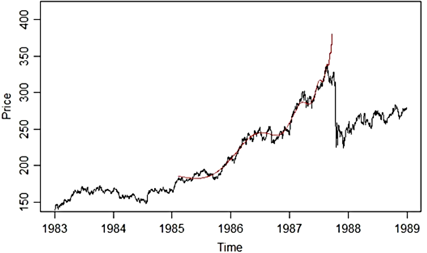
Figure 1. The LPPL-model fitted to the S&P 500 Index prior to the 1987 crash
The LPPL-model has proven useful in predicting the end of speculative bubbles both ex post and ex ante in various markets such as the 2006–8 oil bubble (Sornette et al. Reference Sornette, Woodard and Zhou2009), historical bubbles on the Dow Jones Industrial Average (Vandewalle et al. Reference Vandewalle, Ausloos, Boveroux and Minguet1999), the gold price peak of 2009 (Geraskin and Fantazzini Reference Geraskin and Fantazzini2011) and the real estate market in Las Vegas (Zhou and Sornette Reference Zhou and Sornette2008). However, since there are a lot of markets and bubbles to which the LPPL-model has not yet been fitted, more studies are needed. Also, all previous studies only present results that reinforce the theory, while none has highlighted both the potential and the limitations of the LPPL-model. In addition, no previous study has examined the robustness of the model. By addressing these issues we give ourselves the opportunity to further assess the predictability and the accuracy of predictions of the model, and thereby expand the understanding of the LPPL-model. In the next section, the model, the estimation procedure and the data are presented. Then follow the empirical test and a comparative analysis of the selected bubbles, before our results are summarized.
I
The pattern proposed by the LPPL-model is quantified by the LPPL-equation. When this model was first presented by Sornette et al. (Reference Sornette, Johansen and Bouchaud1996) the equation was defined as
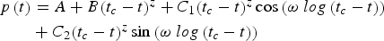
 $$p\left( t \right) = A + B{\left( {{t_c} - t} \right)^z} + C{\left( {{t_c} - t} \right)^z}{\rm cos}\left( {\omega \; log\left( {{t_c} - t} \right) + \varphi} \right)$$
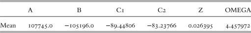
where asset price, p, is a function of time, t, and t c expresses the critical point, the most probable time of a change in regime. The parameter z in the equation controls the strength of the feedback mechanism as well as the amplitude of the oscillations. z must lie between 0 and 1, else we are dealing with some other type of process and not a power law characterized by faster-than-exponential growth. ω denotes the frequency of the oscillations and empirically takes on values between 4.8 and 7.9 (Johansen and Sornette Reference Johansen and Sornette2010). A is a positive parameter which naturally takes on the asset price value of the LPPL-fit at the critical point. The parameter B will in the case of a speculative bubble take on negative values since asset prices are increasing during a bubble, while C must take on values between 1 and -1. φ in the equation simply signifies the direction of the oscillations.
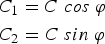
Filimonov and Sornette (Reference Filimonov and Sornette2013) present a modification of the equation where they expand the cosine term of the original equation and rewrite the equation as follows:
 $$\eqalign{p\left( t \right) & = A + B{\left( {{t_c} - t} \right)^z} + {C_1}{\left( {{t_c} - t} \right)^z}\cos \left( {\omega \; log\left( {{t_c} - t} \right)} \right) \cr & + {C_2}{\left( {{t_c} - t} \right)^z}\sin \left( {\omega \; log\left( {{t_c} - t} \right)} \right)}$$
Where
 $$\eqalign{& {C_1} = C\; cos\; \varphi \cr & {C_2} = C\; sin\; \varphi} $$
This transformation has two important implications. Firstly, the transformation decreases the complexity of the fitting procedure since the optimization problem is converted from a four-dimensional space to a three-dimensional space. Secondly, and possibly of even greater importance, the cost function to be minimized now contains a single minimum instead of multiple minima, as long as the model is appropriate for the empirical data. The stability of the model is thereby significantly improved. Due to this transformation the need for complex search algorithms such as a taboo search is eliminated and more simple algorithms, e.g. a Gauss-Newton algorithm, can be used without any reduction in the robustness of the estimation. For these reasons we in this article choose to base our methods on equation (2).
This study is quantitative in its nature and based on a nonlinear least squares estimation with the objective of solving the minimization problem related to equation (2), using a Gauss-Newton algorithm. The nonlinear least squares estimation is conducted over a great number of iterations, using a rolling window technique, where the start and end date of the analyzed time period is changed in between iterations. This is consistent with the recommendations of Sornette et al. (Reference Sornette, Woodard, Yan and Zhou2013) to make the predictions more statistically robust. The estimation procedure returns the two fits with the lowest sum of squared errors for each window of estimation. In each iteration we use all available data up until one month before the actual regime shift in order to examine whether an ex-ante prediction conducted one month before the peak would have yielded an accurate prediction. Henceforth we consistently call this date the last observed date. This procedure yields thousands of results, where the bad fits are separated from the good fits through a set of carefully chosen constraints on the different parameters of the LPPL-equation.
Regarding the parameter ω, measuring the frequency of oscillations, we choose to follow the guidelines proposed by Filimonov and Sornette (Reference Filimonov and Sornette2013) in allowing for values between 3 and 15. When it comes to z, the parameter for feedback and amplitude of oscillations, we do not enforce any further constraints other than the accepted values between 0 and 1. We also constrain B to only take on negative values. In addition, we introduce constraints on the augmented Dickey-Fuller and Phillips-Perron values of the fits to filter out stationary fits which have no explanatory power in predicting the critical points. We only accept fits that are non-stationary at a 1 percent significance level.
By enforcing these constraints we are left with only fits which help explain the regime shift of the bubble, where the end date of each fit signifies the predicted critical point of the bubble, i.e. the point in time at which the asset prices are anticipated to change regime. These end dates are the objects of analysis, where they comprise confidence intervals of critical points, indicating where it is most likely for the analyzed bubble to change regime.
In testing the robustness of the model we proceed by setting the last observed date two months and two weeks prior to the peak, respectively, and repeat the estimation process. Then we can establish whether there is any distinct difference in results based on the last observed date, and whether these results match the theoretical assumption.
II
We chose to focus this study on a selection of bubbles where their historical contexts make them particularly interesting. This might, for example, be when it is well known that the underlying assets were objects of speculation, or when differences in interest rates caused increased capital flows between economies leading to increased anticipation of rising asset prices. We thereby circumvent the problems related to bubble selection based on the drawdown methodology explained by Johansen and Sornette (Reference Johansen and Sornette2010), where the methodology excludes speculative bubbles that do not end in a crash, while it might include exogenous bubbles.
Based on this selection criterion, and due to the lack of previous thorough empirical examination, we select the following eight bubbles to base our analysis upon; the panic of 1907, when financial distress was spread across the Atlantic; the Wall Street crash of 1929, one of the largest financial crises of the twentieth century; the Japanese asset price bubble of the 1980s, one of the most spectacular and speculative bubbles in living memory; the London stock price bubble of the 1990s, where changes in interest rates possibly led to excessive speculation; the emerging markets bubble of the 1990s, where investment trends contributed to excessive price growth in emerging markets; the dot-com bubble of the late 1990s, where an entirely new market led to disproportionate anticipations; the wheat price bubble of the 2000s, where the possible occurrence of speculation has been a topic of discussion; and lastly the Chinese stock market crash in 2015, where investors encouraged by national media invested large amounts, in many cases borrowed money.
The datasets consist of daily closing prices of various well-known stock price indices and a commodity index. Data were retrieved from Thomson Reuters Datastream, except data for the panic of 1907 and the Wall Street crash of 1929, which were retrieved from www.measuringworth.com. The datasets have not been processed by us in any way. We chose to base this study on actual price data since we do not want to process the data more than necessary and since we have found, in a previous study, that the choice of actual versus log-price data does not significantly alter our results (Gustavsson and Levén Reference Gustavsson and Levén2015). We also consider that the use of actual prices is preferable for graphical reasons since this makes the faster-than-exponential growth and thereby the positive feedback mechanism easier to distinguish and understand.
When analyzing the different bubbles we use data from the following indices: for the panic of 1907 and the Wall Street crash of 1929 we use data from the Dow Jones Industrial Average; for the Japanese asset price bubble we use data from the Nikkei 225 Index; for the London stock price bubble we use data from the FTSE 100 Index; for the emerging markets bubble we use data from the Hang Seng Index of Hong Kong; for the dot-com bubble we use data from the Nasdaq Composite Index; for the wheat price bubble we use American Soft Red Winter wheat futures prices; for the Chinese crash we use data from the Shanghai Stock Exchange Composite Index.
III
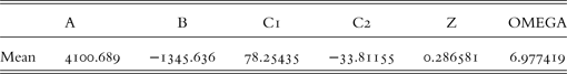
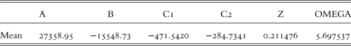
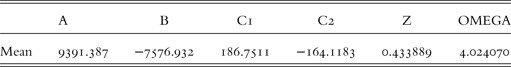
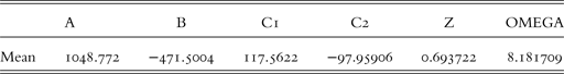
In this section we examine the ability of the LPPL-model to accurately predict the end of speculative bubbles, through modeling of asset price dynamics on a selection of historical bubbles. Highlighted in dark grey in each figure of this section is the 80 percent confidence interval of the critical points, t c , that are the results of the fitting procedure described above. In lighter grey within this interval is a 50 percent confidence interval of critical points. These intervals thus represent the most probable time for a change in regime. The confidence intervals are plotted with the motivation that the date of the regime shift is a highly stochastic process and that the prediction of one specific crash date in fact might be misleading. The median date of the critical points is marked by the (red) vertical line within the confidence interval and gives guidance to where it is more likely for the regime shift to occur. In each graph only a dozen of the resulting LPPL-fits are plotted, regardless of how many resulting fits are produced. We do this for the sake of visibility, while the total number of fitted curves is given in the upper left corner of each figure. The bold black line in each figure illustrates the last observed date, which is where the ex-ante prediction is assumed to be conducted. Due to there in most cases being a lot of fitted curves we, instead of presenting the parameter values for each fit, present the parameter means based on all fits. These values are presented for each estimation conducted one month prior to the peak.
The panic of 1907
In the panic of 1907, the Dow Jones Industrial Average fell almost 50 percent from its peak the previous year. The immediate reason was a retraction of market liquidity by a number of New York City banks and a loss of confidence among depositors. There contagion came from Europe, where London and Paris had decided in 1906 to cut off the credits to Italian banks, after years of speculative investments. Thus, the regime shift came already in 1906. When the financial distress was spread across the Atlantic, the panic spread throughout the US, where many state and local banks and businesses went bankrupt (Kindleberger and Aliber Reference Kindleberger and Aliber1978/2011).
Figure 2 shows the results of a prediction conducted one month prior to the peak. The results are ambiguous. We notice that the model finds two distinct patterns, one with more frequent oscillations that seems to predict an earlier critical point, and one with less frequent oscillations which pushes the interval of predicted end dates to later dates. However, the projection only finds a total of 20 fits, indicating that the prediction should not be taken as a certainty. We observe that the actual peak date of 19 January is captured within the 80 percent confidence interval but occurs months before the 50 percent confidence interval.

Figure 2. The LPPL-model fitted to the Dow Jones Index prior to the panic of 1907

Figure 3a, which shows a prediction conducted two months before the actual peak, gives us a quite different result. Since the model no longer finds any fitted lines matching the pattern with less frequent oscillations we get a much shorter interval of predicted end dates just after the last observed date. Neither the 50 percent confidence interval nor the 80 percent interval captures the actual peak date.

Figure 3a–b. The LPPL-model fitted to the Dow Jones Index prior to the panic of 1907 with different last observed dates
The estimation conducted two weeks prior to the actual peak, as shown in Figure 3b, finds results quite similar to those of Figure 2, with a broad and uncertain interval of predictions. Throughout these three estimations it seems that the model continuously finds oscillations and fits that are not of any significance when trying to predict the regime shift. These results indicate that the model is a poor fit to this time series. However, recall that the model is not supposed to be a good fit for all historic bubbles.
The Wall Street crash of 1929
The stock market crash of 1929 formed the largest financial crisis of the twentieth century. The panic of October 1929 and the Wall Street crash has come to serve as a symbol of the economic contraction that gripped the world during the next decade, during the Great Depression. After a few weeks, the Dow Jones Index had gone down by more than 40 percent. The crash followed on from a speculative boom from the mid 1920s, where steel production, building construction, retail turnover and automobiles registered advanced from record to record. Like the panic of 1907, the roots of the crash in 1929 could be traced to both Europe and the US. On both continents, hundreds of banks and businesses went into bankruptcy in the aftermath of the crash (Kindleberger and Aliber Reference Kindleberger and Aliber1978/2011).
From Figure 4 it is apparent that the asset prices prior to the Wall Street crash follow the characteristic pattern as proposed by the LPPL-model; the prices seem to oscillate around a faster-than-exponential growth where the oscillations become smaller closer to the peak. These price movements act exactly as they are expected to during a speculative bubble, according to the LPPL-framework. It can also be seen from Figure 4 that the actual peak date of 3 September is encapsulated by both the 50 percent and the 80 percent confidence intervals. These are promising results since they indicate that an ex-ante estimation conducted one month prior to the actual peak date would have accurately predicted the upcoming change in regime.

Figure 4. The LPPL-model fitted to the Dow Jones Index prior to the Wall Street crash of 1929
When performing an estimation where the last observed date is two months prior to the peak, we reach similar results to those of Figure 4. It can be seen from Figure 5a that the median date is shifted one day to the right in the graph, while both confidence intervals are broadened compared to the first estimation. These results indicate that an ex-ante prediction conducted two months prior to the peak would have yielded almost the exact same conclusions regarding the upcoming regime shift as those of the estimation performed one month prior to the peak. However, the broadened confidence intervals indicate some additional uncertainty, which is expected when performing an earlier ex-ante prediction.

Figure 5a–b. The LPPL-model fitted to the Dow Jones Index prior to the Wall Street crash of 1929 with different last observed dates
From Figure 5b, where the last observed date is set two weeks prior to the peak, it is evident that both confidence intervals as well as the median are shifted approximately two weeks later compared to the estimation of Figure 4. Since the LPPL-framework suggests that the regime shift should occur when the oscillations reach zero, one possible explanation for this occurrence is that the oscillations are already quite low in amplitude when the last two predictions are conducted. Due to this low amplitude, the model anticipates the number of days after the last observed date needed to reach a zero amplitude to be about the same in both of the last two predictions. Thus, the confidence interval and the median are simply shifted to the right in the graph as we conduct estimations closer to the peak. These results and this possible explanation will be further assessed in the comparative analysis.
The Japanese asset price bubble of the 1980s
The Japanese asset price bubble, a classic example of a speculative bubble, formed in the 1980s due to an increased interest in investments in Japan. This increased interest was in turn attributed to financial liberalization and a relaxed monetary policy followed by the Bank of Japan. The result was a massive inflow of capital from foreign investors. The asset prices plunged in early 1990, which is often attributed to two exogenous events: a tightening of the monetary policy and new credit regulations introduced by the Bank of Japan, imposing lending restrictions on Japanese banks.
When fitting the LPPL-equation to the time series preceding the peak we arrive at the results presented in Figure 6. It can be seen from the figure that the stock prices during this time period follow the characteristics of LPPL. It can also be seen from Figure 6 that both the 80 and 50 percent confidence intervals capture the actual peak date, or regime shift, of 29 December, while the median date is only five days later. This means that if an ex-ante prediction would have been performed on the Nikkei 225 Index one month prior to the actual peak it would have given us a good estimation of the upcoming date of the regime shift.

Figure 6. The LPPL-model fitted to the Nikkei 225 Index during the Japanese asset price bubble of the 1980s

It is evident from Figure 7a that both the start and the end of the confidence intervals are moved roughly one month to the left in the graph compared to the interval in Figure 6, although the 80 percent confidence interval still captures the actual peak date. One possible explanation for this behavior could, as in the case of the Wall Street crash, be that the amplitude of oscillations is already quite low when the predictions are conducted. The confidence intervals will continue to move to the left in the graph when moving the last observed date to the left, as long as the oscillations soon before the last observed date are close to zero. This means that the LPPL-framework would expect the regime shift to occur earlier. Why this speculative bubble lives for so long is difficult to tell. One possibility is that an exogenous trigger might be needed when the oscillations have reached maturity to offset the positive feedback loop and end the bubble. Perhaps in this case there was no negative news big enough to start the downward spiral prior to the implementation of a tightened monetary policy and new central bank regulations. These tentative explanations will be discussed more thoroughly in the comparative analysis below.

Figure 7a–b. The LPPL-model fitted to the Nikkei 225 Index during the Japanese asset price bubble of the 1980s with different last observed dates
From Figure 7b it is apparent that the actual regime shift yet again is captured by the 80 percent confidence interval, while the intervals are moved roughly two weeks to the right in the graph. This is probably for the same reason as above, namely that the oscillations are so far gone when the prediction is conducted.
The London stock price bubble of the 1990s
During the early 1990s the United States Federal Reserve pursued an expansionary monetary policy, which led American and foreign investors to seek alternative investments with higher returns (Blakey Reference Blakey2010). Hence there was a large inflow of capital to European and emerging financial markets. This capital inflow gave birth to a rapid increase in stock prices on these markets. The eventual sudden change of course has been attributed to the Federal Reserve's shift to a more contractionary policy.
In Figure 8, the LPPL-equation is fitted to the FTSE 100 Index during the period preceding the downturn of 1994. It is apparent that the asset prices follow the characteristics of LPPL. It is also evident that the predictions of the LPPL-model in this case yield accurate results, since the actual change in regime on 2 February is captured by both confidence intervals.

Figure 8. The LPPL-model fitted to the FTSE 100 Index during the London stock price bubble of the 1990s
The accuracy of the predictions may be surprising since both the initiation and end of the bubble were most likely influenced by an exogenous factor, the Federal funds rate. Perhaps the initiating shock started a wave of positive feedback where speculation on further increases drove the market to new heights. In line with the results of the Japanese asset price bubble, perhaps the Federal funds rate acted as an exogenous trigger which disrupted the speculative behavior.
When the last observed date is set two months prior to the peak date the intervals of predicted end dates are shifted to the left in the graph, as seen in Figure 9a. These results are reminiscent of those for the Japanese asset price bubble, with the exception that none of the confidence intervals captures the actual peak of 2 February. As in the case of the Japanese asset price bubble, the oscillations are already quite small when the predictions are conducted and this is probably why the confidence intervals are simply moved sideways.

Figure 9a–b. The LPPL-model fitted to the FTSE 100 Index during the London stock price bubble of the 1990s with different last observed dates
When conducting the prediction closer to the peak, as seen in Figure 9b, the intervals of critical points capture the actual peak date.
The emerging markets bubble of the 1990s
During the middle of the 1990s institutional investors, mainly in Europe and North America, found particular interest in emerging markets around the world (Kindleberger and Aliber Reference Kindleberger and Aliber1978/2011). By 1997 the large inflow of capital into several Asian economies led to dramatic rises in asset prices, possibly fueled by speculative behavior. Instability in the Thai economy eventually led to increased perceived risks in emerging markets, and the asset prices plunged in the second half of 1997. The results below are based on the Hang Seng Index of Hong Kong. We have chosen to focus on this index since the Hong Kong Stock Exchange was the largest stock exchange among emerging markets at the time, and probably provides the most reliable data.
It is apparent from Figure 10 that the analyzed time series exhibits clear characteristics of the LPPL-model. The confidence intervals encapsulate the actual regime shift which occurred on 7 August. There is, however, a heavy skew to the left, indicated by the median red line, meaning that the regime shift is more likely to occur during the earlier dates of the interval.

Figure 10. The LPPL-model fitted to the Hang Seng Index during the emerging markets bubble of the 1990s
When the last observed date is set two months prior to the peak date, as in Figure 11a, we observe slimmer confidence intervals of predicted end dates, with the median only a few days earlier compared to the median of the estimation conducted one month prior to the peak. This means that estimations performed one and two months prior to the actual peak would have yielded almost the exact same conclusions regarding the upcoming change in regime. Results that are largely unaffected by when the predictions are conducted are what one wishes to see when examining a bubble.

Figure 11a–b. The LPPL-model fitted to the Hang Seng Index during the emerging markets bubble of the 1990s with different last observed dates
When the last observed date instead is set two weeks prior to the peak, as in Figure 11b, the results are similar to the prediction done one month prior to the peak, with the intervals and the median shifted to the right. This occurrence, yet again, probably has to do with the oscillations already being quite low in amplitude when the predictions are conducted.
The dot-com bubble of the late 1990s
The dot-com bubble of the late 1990s is perhaps one of the most well-known examples of a highly speculative bubble. The establishment of a new market with the advent of internet-based-companies garnered great public interest, which led to drastic increases in asset prices (Lowenstein Reference Lowenstein2004). Concerns about the digital shift to a new millennium contributed to a hype in the computer service industry, including consultancy. The drastic downturn following the peak was not triggered by any particular major event, but was seemingly self-inflicted.
Having the characteristics of a speculative bubble, it does not come as a surprise that the price movements during the dot-com bubble closely followed the patterns of the LPPL-model, as shown in Figure 12. The actual peak date on the Nasdaq Composite Index occurred on 10 March 2000 and thus fits within the 80 percent confidence interval of predictions, but not within the 50 percent interval.

Figure 12. The LPPL-model fitted to the Nasdaq Composite Index during the dot-com bubble of the late 1990s
It can be seen from Figure 13a that when setting the last observed date two months before the peak date the intervals of predictions are comprised of very few curves, and the actual peak date is missed by more than two months. It seems that the model finds only one long oscillation prior to the last observed date and therefore predicts that the bubble will continue for several months. The explanation for why this happens is that the dot-com bubble spans over a quite short period and there is a great deal of information needed for an accurate prediction contained in the price data of the last two months before the regime shift. For the model to accurately predict the regime shift there is a need for more data closer to the peak. When conducted one month before the crash, as in Figure 12, the data include a second oscillation, thus allowing the estimation to find a regime shift closer to the observation date. Without these data the model is unable to anticipate how rapidly the oscillations actually are decreasing in size, which is crucial for the prediction.

Figure 13a–b. The LPPL-model fitted to the Nasdaq Composite Index during the dot-com bubble of the late 1990s with different last observed dates
When the last observed date is set two weeks before the actual peak date, as in Figure 13b, the results are similar those of Figure 12, although the intervals are shifted slightly to the right. The total number of fitted curves is now higher compared to when the prediction is conducted both one and two months before the peak. This is what one might expect when a bubble ranges over a short period of time and the information contained in the last few months is of great significance for the prediction.
The wheat price bubble of the 2000s
During the period 2006–8 the price of wheat futures increased more than threefold to a high of 1,280 US cents per bushel. Whether widespread speculative behavior was the reason behind this rapid price increase or not has been a topic of discussion after the drastic downturn in prices during 2008. Most probable is that the wheat prices were affected by several factors including rising demand for food, climate change, high oil prices, increased interest in alternative use of land through biofuels, but also speculative behavior (Robles et al. Reference Robles, Torero and von Braun2009). As a result of the global financial crisis starting in 2007 and the associated credit crunch with more restrictive lending, overall speculative behavior saw a major drop as capital became harder to access (Mizen Reference Mizen2008). The downturn in wheat prices was probably a result of the credit crunch, although other factors possibly could have been influential as well.
Although the bubble in wheat futures is said to have begun in 2006 the model only finds fits starting in April 2007. For this reason we only present the shorter period between April 2007 and March 2008 in Figure 14 and 15a–b. It is possible that the prices started to rise in 2006 but the actual herding behavior commenced in 2007. The futures prices have two peaks, where we have chosen to define the second peak as the regime shift, since it is at this time that the growth rate of the prices is dramatically changed. It can be seen from Figure 14 that the LPPL-model yields a quite inaccurate prediction where the actual peak date is not encapsulated by the confidence intervals and the median date is about two weeks prior to the peak date. It can also be observed that the price of wheat futures, despite the inaccurate prediction, closely follows the characteristic patterns proposed by the LPPL-model leading up to the last observed date.

Figure 14. The LPPL-model fitted to wheat futures prices during the wheat price bubble of the 2000s
A question that arises when examining Figure 14 is how it is possible for the model to miss the actual regime shift with such significance despite the fits of the curves being quite accurate. It seems that the oscillations are so far gone when the prediction is conducted that they indicate a regime shift close to the last observed date, while the movements after the last observed date are not possible to explain from the underlying theory of the LPPL-model.
Figure 15a illustrates that an ex-ante prediction conducted two months before the regime shift yields results indicating that the change in regime should occur right after the last observed date. This prediction is, yet again, probably due to the fact that the oscillations already have reached maturity and are quite small when the prediction is conducted.

Figure 15a–b. The LPPL-model fitted to wheat futures prices during the wheat price bubble of the 2000s with different last observed dates
It is apparent from Figure 15b that the model yields more accurate critical points when the ex-ante prediction is assumed to be conducted two weeks before the actual change in regime. However, the 80 percent confidence interval just barely captures the actual peak date while the 50 percent interval does not. Yet again the oscillations are quite small when the prediction is conducted and therefore the change in regime is expected to occur just after the last observed date.
The Chinese stock market crash in 2015
The Chinese stock market crash began with the popping of the stock market bubble on 12 June 2015. Within one month, a third of the value of A-shares on the Shanghai Stock Exchange was gone and half of the listed firms filed for a trading halt in an attempt to prevent further losses. Despite efforts by the government to reduce the fall, values of Chinese stock markets continued to drop. After three stable weeks the Shanghai index fell by 8.5 percent on 24 August, dubbed Black Monday, wiping out hundreds of billions of dollars in market capitalization. This event marked the largest biggest one-day fall since 2007. Commodity prices fell into territory not seen since 1999, and the contagion infected Western markets.Footnote 1 One reason for the bubble was a herding behavior among domestic investors. The Chinese economy was expansive and enthusiastic individual investors, encouraged by state-owned media, invested in stocks, often using borrowed money. Since the prospects were high, the value of the stocks often exceeded the rate of growth and profits of the very companies. The inflated prices also reflected a long history of high market volatility in China, typical for emerging markets in transition economies. The bumpy prices and the burst of the bubble revealed structural imbalances in the Chinese economy.Footnote 2
From Figure 16 we can see that the bubble preceding the Chinese stock market crash follows the pattern of the LPPL-model closely and that the median date ends up just a few days ahead of the actual peak on 12 June. Both confidence intervals are quite tight and encapsulate, or are close to encapsulating, the actual change in regime.

Figure 16. The LPPL-model fitted to the Shanghai Stock Exchange Composite Index prior to the Chinese stock market crash in 2015
When conducting a prediction two months prior to the peak we retrieve the fits of Figure 17a, where it is apparent that the period prior to the last observed date follows the LPPL-model pattern closely and that the model is quite uncertain about what is going to happen next. For these reason we end up with widely scattered predicted end dates, and thus wide confidence intervals. Both the 80 percent and the 50 percent confidence intervals capture the actual peak, while the median is more than a month off.

Figure 17a–b. The LPPL-model fitted to the Shanghai Stock Exchange Composite Index prior to the Chinese stock market crash in 2015 with different last observed dates
The prediction conducted two weeks prior to the peak, as in Figure 17b, yields an accurate prediction, where both confidence intervals capture the actual peak date and the median date ends up just one day after the peak.
IV
We find that most of the bubbles analyzed behave in accordance with the expected characteristics of the LPPL-model. The price movements leading up to the regime shift are characterized by faster-than-exponential growth and show clear oscillatory patterns where the oscillations decrease in amplitude leading up to the regime shift. The smaller oscillations close to the regime shift are in some cases difficult for the model to fit perfectly, although it is clear that these oscillations in general are smaller than the earlier oscillations, and that deviations from the patterns proposed by the LPPL-model are uncommon.
The most apparent deviation from the expected behavior of the model is the results for the panic of 1907. We previously noted that the prediction yields inaccurate and uncertain results with poor robustness, which could be used as an argument against the assumptions of the model. However, recall that the theory of the model only applies to bubbles that are driven by the endogenous factors of the LPPL-framework and does not claim that all bubbles follow this pattern. We instead consider the results to be an indication that the bubble preceding the panic of 1907 was driven not by endogenous super-exponential growth but by other factors. Thus we conclude that the basic assumptions of the LPPL-model are legitimate, since the suggested patterns are possible to observe on markets during bubble periods.
The reasoning behind why asset prices during bubble periods in theory should increase faster-than-exponentially and simultaneously oscillate around this trend is well established in the LPPL-framework. However, what is less discussed in the literature are the reasons why the oscillations decrease in amplitude as the bubble approaches its regime shift. Previous studies have explained this behavior as strictly empirical. We imagine that the earlier oscillations during a bubble are results of investor mentality alternating between optimism and pessimism, while one possible explanation for the decreasing amplitude is that as asset prices reach greater heights, so does the market anxiety. It is safe to assume that as investors get more anxious they are less confident in their positions, while at the same time afraid of missing out on further increases, resulting in short periods of market sell-outs and buy-ins. For this reason there are periods with ups and downs as the bubble approaches its peak. Despite these movements being quite large in a short time frame, compared to the earlier oscillations during the bubble they are small. This behavior would result in more frequent oscillations with lower amplitude as the bubble gets older. This reasoning is in line with the theory proposed by Abreu and Brunnermeier (Reference Abreu and Brunnermeier2003), according to which rational arbitrageurs ‘test the market’ to find out whether many investors, like themselves, have realized that the asset prices are overvalued.
One recurring observation of the results is the apparent influence of exogenous factors on the regime shift of a bubble. For example, the downturn following the Japanese asset price bubble has been attributed to a tightened monetary policy and new credit regulations, while the regime shift of the emerging markets bubble was influenced by the Thai crisis. Despite these exogenous influences the predictions of the model are quite accurate, which is unexpected since the model obviously cannot predict the occurrence of exogenous events. Additionally, in some cases we observe that the entire interval of predicted end dates is shifted when moving the last observed date, calling into question the nature of the model's predictive ability. These results are problematic for the prediction of regime shifts since the actual peak date is unknown when conducting ex-ante predictions. We propose a couple of possible explanations for the exogenous influence on the regime shifts.
One possibility is that the exogenous events that seem to be plausible explanations for the regime shifts are accredited more influence than is justified. Since it is difficult to measure speculative behavior, the influence of endogenous speculative growth might be mitigated in favor of more easily observable exogenous events. For example, in the case of the London stock market bubble the regime shift seems to have been the effect of unsustainable speculative behavior based on the results of the LPPL-curves, but the prevailing explanation for the downturn is the more easily observed external change in the interest rate. The disregarding of speculation in favor of an exogenous trigger may explain the apparent influence of exogenous factors although it does not serve as a satisfactory explanation for why the confidence intervals of predicted end dates in many cases are shifted when the last observed date is changed.
Another possible explanation is that the endogenous speculative growth and the exogenous trigger events complement each other. We propose that the LPPL-model patterns by themselves are not enough to explain the end of a speculative bubble. Rather there is a need for an exogenous event to trigger the regime shift after the oscillations have reached maturity. We find this to be the most feasible explanation since it also explains the quite frequently occurring shift in the intervals of predicted end dates. Consider, for example, the case of the Japanese asset price bubble. From Figure 6 and Figure 7a–b it seems that the oscillatory patterns of the LPPL-curves become very small and probably reach maturity in late 1988. By setting the last observed date two months prior to the peak, the model then concludes that the time series is sensitive to a regime shift just following the last observed date. The fact that the asset prices continued to grow for two months more indicates that there was no exogenous event large enough to trigger the regime shift during this period. In fact, the model in this case will predict the regime shift to occur quite soon after the last observed date when predicting the outcome as early as in late 1988. In this particular case it took until the implementation of a tightened monetary policy and stricter central bank regulations in late 1989 for the herding behavior to be disrupted. At this point the asset prices had risen a great deal, while the impending downturn was more severe.
Our hypothesis is strengthened by the logical assumption that for speculators to stop buying and start selling, something more than endogenous factors is needed. During bubble periods asset prices continue to rise due to anticipation of further price increases. For the prices to take a downturn, or change regime, the investors have to change their expectations with regard to anticipating decreasing asset prices. It is easy to assume that this does not happen by itself; an exogenous event is needed to disrupt the herding behavior and the investors’ anticipations. In some cases this disruption might crystallize as reversed speculative behavior, where investors sell because they are anticipating decreasing asset prices, causing a crash on the market. If no exogenous event occurs the herding behavior and increasing asset prices will continue until big enough negative news reaches the market. On the other hand, if such an exogenous event occurs before the speculative behavior has reached maturity, i.e. when the oscillations are still quite large in amplitude, the prices will not fall drastically since they are not sufficiently overvalued to begin with. We expect a dip in prices since they still are affected by exogenous shocks, although the asset prices quickly return to the trend and thereafter continue to rise in accordance with the LPPL-model patterns.
This reasoning is in line with the work of Abreu and Brunnermeier (Reference Abreu and Brunnermeier2003), who argue that rational arbitrageurs ‘ride the bubble’ even though they are aware of its existence and that it eventually has to burst. The rational arbitrageurs choose to stay in the market because they do not know whether they have acquired this information early or late relative to other rational arbitrageurs. These agents await the next negative exogenous shock events and choose to get out of the market when the perceived probability that the bubble will burst is sufficiently high. Our hypothesis suggests that the model's ability to predict the bursting of bubbles is not as strong as has been claimed in previous studies, since it actually predicts periods when asset prices are especially sensitive to exogenous events. Therefore, the results of all estimations have to be interpreted in a more careful manner. When conducting an ex-ante prediction and interpreting the results, the predicted critical points should not be interpreted as best estimates of a change in regime, but rather as the start of a period when the asset prices are more sensitive to negative external events. However, as our empirical results underline, the model still has the capacity to accurately predict regime shifts. Negative exogenous events occur during most time periods and quite frequently, leading to the conclusion that a regime shift usually closely follows when the oscillations have reached maturity. The asset prices do not change regime due to negative exogenous events earlier since the oscillations at this point have not reached far enough. Therefore, the high frequency of negative exogenous events can explain the accuracy of the LPPL-model in most cases.
Before going into what we have found on the robustness of the LPPL-model it is important to consider what robustness actually means in this context. Consider an ex-ante prediction conducted two months before the actual regime shift. For the model to yield similar results when conducting an ex-ante prediction one month later, it is a prerequisite that the price movements during the period in between have followed the predicted LPPL-fits of the earlier estimation. If this is not the case the new prediction will yield different results than those of the earlier prediction. We can observe this on several of the bubbles analyzed where the results cannot be considered robust. A representative example is that of the dot-com bubble, where the predictions yield different results since price movements in between the dates of prediction are contradictory to the LPPL-model patterns of the earlier prediction. A counter-example is that of the emerging markets bubble, where the price movements in between the dates of prediction follow the first LPPL-fits closely. The results of the emerging markets bubble are clearly to be considered robust.
Even though the results of the emerging markets bubble as well as, at least to some degree, the Wall Street crash of 1929 yield robust results, the results in general cannot be regarded as robust since most of the bubbles examined exhibit predictions that are dependent on the time of prediction. Why the predictions regarding the dot-com bubble are not robust is quite easy to tell. The bubble in this case spreads over a quite short time interval while the asset prices increase very rapidly. Due to this there is a great deal of information contained in the price data of the last few months, why the earlier prediction does not capture the actual trend and its oscillations leading up to the regime shift. The same reasoning applies for the Shanghai stock market bubble, also a bubble spanning over a quite short time period. The Japanese asset price bubble, the London stock market bubble and the wheat price bubble all seem to suffer from the same condition, where the results of the different predictions cannot be regarded as robust.
Instead of drawing the conclusion that the LPPL-model is lacking predictive ability due to this non-robustness, we stick to our hypothesis presented earlier. The reason why these predictions are so dependent on the time of prediction is that the oscillations are so far gone when the predictions are conducted, and the market is awaiting negative news big enough to disrupt the upward trend. For this reason, the predicted end dates appear just after the last observed date. That the model does not yield robust results is of no major significance, since this is totally logical if the estimation results are interpreted as predictions as to when the asset prices start being more easily influenced by exogenous factors.
Given this newfound interpretation one may ponder upon the ex-ante usability of the LPPL-model. The different estimations of the Chinese stock market crash shed light on this question since they reveal how the model can be used to examine bubbles ex ante by monitoring price developments through continuous estimations. At the estimation two months prior to the peak date the investor can see that an LPPL-model pattern is forming and that there are several possible trajectories the future price development can take. One month later the investor observes the course that the prices actually took, and can conclude that the peak is near. If the investor chooses to wait another two weeks before exiting the market they will notice that the model still determines that the end is near. When performing continuous estimations, results like these are exactly what you want to see, since they all point in the same direction and form a basis for an investment strategy. The reasons why the ex-ante usability becomes so clear in this case is that the Chinese stock market crash was quite a short bubble and the usage of estimations conducted one month, two months and two weeks prior to the crash, respectively, suits a shorter bubble better than a long one. For the same reasons the ex-ante usability is also quite clear for the dot-com bubble. We propose that future research should be more focused on assessing the ex-ante usability of the LPPL-model, especially through monitoring a larger number of estimations for each bubble, with a longer interval in between the different estimations.
V
We have investigated the ability of the LPPL-model to accurately predict the end of speculative bubbles on financial markets. Previous studies have only presented results where the predictions turn out to be successful. Through this study we are first to highlight both the potential and the limitations of the LPPL-model. We have done so by applying the model to time series of eight bubbles, chosen based on their historical context. Our empirical results reinforce the underlying theory of the model that asset prices during bubble periods oscillate with decreasing amplitude around a faster-than-exponential growth. We find that the predictions of the LPPL-model in most cases are quite accurate, where the actual peak date is encapsulated by the confidence intervals of critical points. The robustness of the model, however, can be questioned since the predictions seem to be dependent on when they are conducted.
One recurring observation is that asset prices continue to rise with small oscillatory patterns even after the predicted regime shift. We suggest that this is due to there being an interaction between exogenous and endogenous influences, where an exogenous factor acts as a trigger and is needed for the speculative behavior to be disrupted, thus changing the regime. With this motivation we propose that the results of the LPPL-model should be interpreted differently. We argue that the interval of critical points is not a prediction of the regime shift itself, but rather a prediction of when the asset prices are especially sensitive to influences of exogenous factors. The interval thus gives an indication of the point in time after which a negative exogenous factor is enough to disrupt the speculative behavior. The reason why the LPPL-model yields accurate predictions in most cases is due to these exogenous events occurring quite frequently. When no such event occurs the asset prices continue to rise, although the oscillations have reached maturity. To conclude, our study has shown that the LPPL-model has the ability to predict sensitivity to exogenous events ex ante.


