Formulation of problem

Active phased antenna array diagnosis problem is carried out on the basis of the inverse problem solution and can be reduced to the finding of array elements’ amplitudes and phases. The geometry of the problem is shown in Fig. 1. Radius vector r_n specifies the position of n-th (n = 1,2, …, N) radiating element located in the aperture plane S _A, r_m is the position of m-th (m = 1,2,…, M) measurement point in the measurement surface S _M. The field of each element is modeled by a set of elementary electric and magnetic dipoles, which are located at ${\bf r}_{kn}^e $ and ${\bf r}_{kn}^m $, k = 1,2, …, K. Current distribution of the dipoles is given as:

(1)$$\eqalign{{\bf j}{\kern 1pt} _T^e ({\bf r},\omega ) = &p_{kn}^e \delta ({\bf r}-{\bf r}_{kn}^e ){\bf p}_{0k}^e \cr {\bf j}{\kern 1pt} _T^m ({\bf r},\omega ) = &p_{kn}^m \delta ({\bf r}-{\bf r}_{kn}^m ){\bf p}_{0k}^m,} $$

where $p_{kn}^e {\bf p}_{0k}^e $ and $p_{kn}^m {\bf p}_{0k}^m $ are the vector dipole moments, and ${\bf p}_{0k}^e $ and ${\bf p}_{0k}^m $ are the unit vectors that define the orientation of k-th dipole.

Fig. 1. Geometry of the problem.

The field of the n-th element at the m-th measurement point can be found as shown in [Reference Hansen17]:

(2)$${\bf E}_{Dn}({\bf r}_{mn},\omega ) = {\bf E}_{Dn}^e ({\bf r}_{mn},\omega ) + {\bf E}_{Dn}^m ({\bf r}_{mn},\omega ),$$

where

(3)$$\eqalign{{\bf E}_{Dn}^e ({\bf r}_{mn}) = &\displaystyle{{ik_0Z_0\exp (-ik_0r_{mn})} \over {4\pi r_{mn}}} \cr &\quad \times \left[ {\sum\limits_{{\rm k} = 1}^{N_{\rm }} {\,p_{kn}^e \exp \left( {i\,k_0{\kern 1pt} {\bf r}_{kn}^e {\bf r}_{n0}} \right)\left[ {\left( {{\bf p}_{0k}^e {\bf r}_{n0}} \right){\bf r}_{n0}-{\bf p}_{0k}^e } \right]} } \right] \cr = &{\tilde {\bf E}}_{Dn}^e ({\bf r}_{mn})\displaystyle{{\exp (-ik_0r_{mn})} \over {r_{mn}}}} $$

and

(4)$$ \!\! \eqalign{{\bf E}_{Dn}^m ({\bf r}_{mn}) = &-\displaystyle{{ik_0\exp (-ik_0{\kern 1pt} r_{mn})} \over {4\pi r_{mn}}} \times \left[ {\sum\limits_{k = 1}^{K_{\rm }} {\,p_k^m \exp \left( {ik_0{\kern 1pt} {\bf r}_k^m {\bf r}_{n0}} \right)\left[ {{\bf p}_{0k}^m \times {\bf r}_{n0}} \right]} } \right] \cr = &{\tilde {\bf E}}_{Dn}^m ({\bf r}_{mn})\displaystyle{{\exp (-ik_0r_{mn})} \over {r_{mn}}},} $$

where k ₀ is the wave number, $r_{mn} = \vert {{\bf r}_m-{\bf r}_n} \vert $ ‒ distance from the element to the measurement point,${\bf r}_{n0} = {\bf r}_{mn}/r_{mn}$, and it is taken into account that r _mn ≫ $\vert {{\bf r}_{kn}^e} \vert $ and r _mn ≫ $\vert {{\bf r}_{kn}^m} \vert $ (see Fig. 1). Assuming that the dipole moments in (3) and (4) are normalized, the radiated field (2) of the n-th element excited by the current with complex amplitude x _n can be found as

(5)$$\eqalign{{\bf E}_{Dn}({\bf r}_{mn}) = &x_n\big( {{ \tilde{ \bf E}}_{Dn}^e ({\bf r}_{mn}) + { \tilde {\bf E}}_{Dn}^m ({\bf r}_{mn})} \big) \displaystyle{{\exp (-ik_0r_{mn})} \over {r_{mn}}} \cr = &x_n{\bf E}_n(\theta, {\kern 1pt} \varphi )\displaystyle{{\exp (-ik_0r_{mn})} \over {r_{mn}}},} $$

where ${\bf E}_n(\theta {\rm,} {\kern 1pt} \varphi )$ is the n-th element field (or far-field pattern) when the excitation current amplitude is unity. If the receiving far-field pattern of the probe ${\bf h}(\theta, \phi )$ is known, the antenna array diagnosis problem can be written in matrix form

(6)$${\bf U} = {\bf Ax}$$

where ${\bf x} = (x_1,x_2, \ldots, x_N)^T\in {\open C}^N$ is an excitation vector, ${\bf U} = (U_1,U_2, \ldots, U_M)^T\in {\open C}^M$ is the measurement vector, i.e. complex amplitudes of voltage registered by the probe, and elements of the measurement matrix ${\bf A}\in {\open C}^{M \times N}$ can be found as

(7)$$a_{mn} = \displaystyle{{U_m} \over {x_n}} = {\bf E}_n(\theta _{mn},{\kern 1pt} \varphi _{mn}) \cdot {\bf h}({\theta} ^{\prime}_{mn},{\kern 1pt} {\varphi} ^{\prime}_{mn})\exp (-ik_0r_{mn})/{\kern 1pt} r_{mn}$$

The definition of angles θ, φ, θ′, and φ′ is shown in Fig. 2.

Fig. 2. Geometry of coordinate systems used for n-th radiating element and m-th position of the probe located at the point P.

This formulation is correct for any array geometry and measurement surface S _M. It is also applicable to similar problems that can be reduced to the reconstruction of electric and/or magnetic currents, in the frequency domain or time domain [Reference Kuznetsov, Baev, Gorbunova, Konovalyuk, Thomas, Smartt, Baharuddin, Russer and Russer18]. Conventional methods require M ≥ N to solve (6), i.e. a full set of measurements is required. Due to several reasons, the measurement matrix A is ill-conditioned, so the convergence and accuracy of the solution degrade when the dimensionality of the problem grows [Reference Bucci, Migliore and Panariello6].

Solution of CS problem

It is assumed that the excitation vector is sparse, i.e. the number of non-zero components K is significantly lower than total number of its elements N. For an array that has low number of defect elements, a vector that is a difference between defect array (AUT) and reference array (non-defect) can be found x = x_r − x_d. Then (6) can be rewritten as

(8)$${\bf U}_d-{\bf U}_r = {\bf A}({\bf x}_d-{\bf x}_r)$$

(9)$${\bf U} = {\bf U}_d-{\bf U}_r,\quad {\bf x} = {\bf x}_d-{\bf x}_r$$

Excitation vector x in (9) (see Fig. 3) corresponds to a “sparse” array that consists of a small number of radiating elements.

Fig. 3. An illustration of 10 × 10 “sparse” array construction.

Note that the reference array excitation vector can be found by using the conventional diagnosis methods or by means of numerical modeling. If the number of measurements M is smaller than the number of elements N (the goal of using CS-based methods), the problem (8) is ill-posed and a regularization procedure is required. Usually some kind of a priori information about the solution is used, e.g. the sparseness of x for the CS-based methods. There are different ways to exploit the sparseness of x [Reference Migliore9], for example, using the ℓ₀ norm:

(10)$$\min \left\Vert {\bf x} \right\Vert_0:\quad \left\Vert {{\bf Ax}-{\bf U}} \right\Vert _2 \lt \varepsilon, $$

or using a more convenient ℓ₁norm, which leads to a convex minimization problem:

(11)$$\min \left\Vert {\bf x} \right\Vert _1:\quad \left\Vert {{\bf Ax}-{\bf U}} \right\Vert _2 \lt \varepsilon, $$

where $\left\| \ldots \right\|_2$ is Euclidean norm, $\left\Vert {\bf x} \right\Vert_1 = \sum\limits_{n = 1}^N {\vert {x_n} \vert } $ is ℓ₁norm, ε is related to the noise affecting the data. The constrained minimization problem (11) can be rewritten as a ℓ₁/ℓ₂ minimization problem

(12)$$\mathop {\min} \limits_{\bf x} \left\Vert {{\bf Ax}-{\bf y}} \right\Vert _2^2 + \mu \left\Vert {\bf x} \right\Vert _1,$$

which can be efficiently solved using different iterative algorithms, e.g. YALL 1 [Reference Yang and Zhang19] or NESTA [Reference Becker, Bobin and Candes20,Reference Nesterov21].

The reliability and precision of solution depend not only on the signal-to-noise ratio (SNR), but also on the measurement matrix, i.e. the positions of measurement points. If a measurement matrix satisfies the so-called restricted isometry property (RIP) [Reference Migliore9,Reference Rauhut10], then the excitation vector can be reliably reconstructed with high precision. Calculation of RIP requires proof for all K-sparse x vectors, which is usually impractical. For far-field array diagnosis, an approach to the deterministic selection of measurement points is presented in [Reference Li, Deng and Migliore13]. In a near-field diagnosis case discussed in [Reference Pinchera and Migliore14], a 368-element circular array is effectively diagnosed using 24 measurement points, whose positions were determined by numerical trials.

Even if the optimal positions of the probe are found, there still are other issues that need to be solved before CS-based methods could be used in practice. They are described in the next section.

Low reconstruction accuracy

First modification of the method addresses an issue with exact values of measurement matrix A. The only practically feasible way of obtaining A with high precision implies direct measurements of the field of every single element at every measurement point (7). This process is very time-consuming and requires AUT to be placed exactly in the same position as a reference array. This leads us to the two-step algorithm. In the first step, the radiating elements are separated into two groups: normally operating elements and potentially defect elements using CS-based diagnosis. The second step is required to separate the defect elements and operating elements from the set of potentially defect elements. To do so, the additional measurement set is conducted at a selected measurement point m (or a set of selected additional measurement points, see Fig. 4), for which a _mn, n = 1,…, N, is known with required high accuracy.

Fig. 4. Geometry of acquisition for additional measurements.

For each potentially defect element, the excitation phase is increased (using phase shifters of AUT) by the specified value Δφ, e.g. 180°, leaving the excitations of other elements unchanged. For k-th defect element, the complex amplitudes of the measured field at the measurement point can be found as

(13)$$\eqalign{\dot{U}_{\Sigma 1}^k = \dot{U}_{\Sigma 0}^k + {\dot{U}}^k = &\sum \limits_{n = 1,\;n \ne k}^N {\big( {\dot{U}_n^d -\dot{U}_n^r} \big) } + \dot{U}_k^d -\dot{U}_k^r \cr \dot{U}_{\Sigma 2}^k = \dot{U}_{\Sigma 0}^k + {{\dot{U}}^{\prime k}} = &\sum\limits_{n = 1,\;n\ne k}^N {\big( {\dot{U}_n^d -\dot{U}_n^r} \big) } + \dot{U}_k^d \times \exp (i\Delta \varphi )-\dot{U}_k^r,} $$

where $\dot{U}_{\Sigma 1}^k $, $\dot{U}_{\Sigma 0}^k $, and $\dot{U}^k$ are the complex amplitudes (before changing the phase of k-th element) of the measured field, field of all elements except k-th element and field of k-th element only, respectively. $\dot{U}_{\Sigma 2}^k $ and ${\dot{U}}^{\prime k}$ are the complex amplitudes (after changing the phase) of the measured field and of k-th element field, respectively. Transforming (13), the field produced by k-th defect element can be found as

(14)$$\dot{U}_k^d = \displaystyle{{\dot{U}_{\Sigma 1}^k -\dot{U}_{\Sigma 2}^k} \over {1-\exp (i\Delta \varphi )}}$$

Note that $\dot{U}_{\Sigma 1}^k -\dot{U}_{\Sigma 2}^k $ may be zero in case the amplitude of k-th element is zero, or in case of phase shifter failure when Δφ = 0. The element will be classified as a defect in both cases.

The complex amplitude of k-th element excitation can be found from (6) as

(15)$$\dot{x}_k^d = \displaystyle{{\dot{U}_k^d} \over {{\dot{a}}_{mk}}}$$

or, if using expression (7):

(16)$$\dot{x}_k^d = \displaystyle{{\dot{U}_k^d r_{mk}\exp (ik_0r_{mk})} \over {h({{\theta} ^{\prime}}_{mk},{{\varphi} ^{\prime}}_{mk})E(\theta _{mk},\varphi _{mk})}}$$

Thermal instability of the array

Second modification of the method addresses the issue of thermal instability of the array. Changes in excitation are usually modeled in the same way as thermal noise (e.g. [Reference Pinchera and Migliore14]), but thermal instability error has a non-zero mean value because changes in temperature lead to approximately the same change of amplitude and phase of all elements. It means that vector ${\bf x} = {\bf x}_d-{\bf x}_r$ is no longer sparse and non-defect elements could be categorized as a defect.

To solve this problem we assume that all elements change their amplitudes and phases equally. This assumption is true when temperature changes only slightly (several °C) and there is no significant variation in temperature across the array. In practice, it means that the reference and defect arrays are the same, e.g. when the reference array is measured, then tested (mechanically/thermally) and then is measured again at the same thermal conditions as before to check whether any active elements have failed.

In this case, the measured field of AUT ${\bf U}_d^m $ can be found as

(17)$${\bf U}_d^m = p_c {\bf U}_d,\quad p_c = a_c\exp (i\varphi _c),$$

where p _c is a correction coefficient and U_d is the field that would be measured in the absence of thermal instability. Then equation (9) takes the form

(18)$${\bf U} = \displaystyle{{{\bf U}_d} \over {\,p_c}}-{\bf U}_r,\;{\bf x} = \displaystyle{{{\bf x}_d} \over {\,p_c}}-{\bf x}_r$$

To determine the correction coefficient p _c the minimization problem (12) should be solved for different values of p _c.

(19)$$\mathop {\min} \limits_{\,p_c} \left\Vert {{\bf A}{\bf x}_f-\lpar {{\bf U}_d^m p_c^{-1} -{\bf U}_r} \rpar } \right\Vert _2^2 + {\rm \mu} \left\Vert {{\bf x}_f} \right\Vert _1,$$

where x_f is a solution of (12) for a given value of p _c. Function minimized in (19) is convex, in the absence of noise its minimum corresponds exactly to correction coefficient p _c.

It should be noted that all CS methods are based on a priori information about the solution (the assumption that the solution is sparse). Hence the proposed procedure is only useful when (17) is at least approximately true. If thermal changes also affect the phase-distribution network, or if AUT is so large that the temperature is different across the array, then the algorithm cannot improve the solution. In this case, more precise a priori information or more measurements are required to reconstruct the excitation successfully.

Model of the array and experiment parameters

A planar rectangular 10 × 10 array of open waveguide elements is considered, the field of the array was simulated with FDTD. While CS-based diagnosis methods do not strictly require the measurement surface to be planar, it is common to measure the field of a planar array on a plane parallel to the aperture [Reference Wang7]. To ensure that the measurement points are in the far-field region of any radiating element (but not in the far-field of the array itself), we have chosen the distance between the measurement plane and the aperture of the array to be equal 3λ, where λ is the operating wavelength. To show the ability of CS-based methods to solve the underdetermined problem (9), we have chosen the number of measurements lower than the number of elements, in our case M = 35. It is possible that this number could be improved if another measurement geometry was used, but, as noted in the Introduction, the problem of optimal measurement point selection in the near-field case has not been solved yet.

The effectiveness of a diagnosis method may be characterized in many different ways, but in our case, two values are of particular interest: failure identification success rate (FISR) and PFD. FISR is the probability of locating all defect elements, and PFD is the average number of false detections per a non-defect element of the array:

(20)$${\rm PFD} = \displaystyle{{{\rm Average}\;N\;{\rm of}\;{\rm false}\;{\rm detections}\,{\rm in}\;{\rm solution}} \over {N\;{\rm of}\;{\rm non\hyphen defect}\;{\rm elements}}}$$

The accuracy and precision of the method were also investigated. Since l ₁-based reconstruction methods are known to underestimate high-amplitude components [Reference Selesnick22,Reference Wei, Zhang, Han, Xu, Hong and Wu23], we have computed both the mean value of the error and its standard deviation (SD).

The excitation of the reference array was uniform. In a defect array, 3–10 (to keep the number of defects K much lower than the number of elements N) defect elements with excitations specified in Table 1 were present. All non-defect elements have an amplitude of 1 and phase 0°.

Table 1. Excitations of defect elements

The radiation pattern E_n of n-th radiating element in equation (7) is not always known exactly, and elements of a calculated measurement matrix may differ from the measured ones. In order to determine how errors in the measurement matrix influence the solution, diagnosis problem (12) was solved using three different measurement matrices. The “exact” (or “reference”) measurement matrix A_R is acquired by simulating sequential excitation of every single element. For the “simplified” measurement matrix A₀ all elements were assumed isotropic (E_n = 1 for all n). The “approximate” measurement matrix A₁ was calculated using a quasi-analytical far-field pattern of an open waveguide E_n.

Positions of the elements and measurement points are shown in Fig. 5.

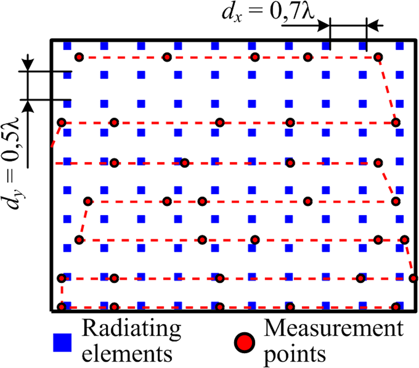
Fig. 5. Positions of radiating elements and measurement points.

The n-th element was considered a defect when the absolute value of x _n (n-th component of the vector ${\bf x} = {\bf x}_d-{\bf x}_r$) was larger than a certain threshold. In this paper, this threshold was set to 0,1, which corresponds roughly to ±1 dB amplitude error (to detect defects of discrete attenuators with a least significant bit of 0.5…1 dB) or ±6° phase error (to detect defects of 6-bit discrete phase shifters with a least significant bit of 5625°).

Finally, we assume that the accuracy of amplitude and phase measurement is about ±5% and ±2°, respectively. This accuracy roughly corresponds to an SNR of 40 dB stated in [24].

All parameters of the model are combined in Table 2.

Table 2. Parameters of the model

Results of diagnosis without correction

For a given number of defects, FISR and PFD were estimated by repeating the identification procedure 2000 times (100 different distributions of defect elements, 20 different realizations of white Gaussian noise for each distribution). Results of diagnosis (FISR and PFD) in thermally stable conditions are shown in Figs 6(a) and 6(b).

Fig. 6. Characteristics of the diagnosis method for a 10 × 10 array of open waveguide elements with 3λ distance to measurement plane: (a) failure identification success rate (FISR) and (b) probability of false detections (PFD). A_R – results acquired using the reference measurement matrix, A₀ – “simplified” measurement matrix, A₁ – “approximate” measurement matrix.

As it could be expected from the results presented in [Reference Pinchera and Migliore14], FISR decreases with the number of defect elements. For a small number of defects, FISR is high no matter what measurement matrix was used; the only real difference is PFD. For 10 defects, PFD obtained using A_R and A₀ differ more than 10 times.

The accuracy of amplitude and phase reconstruction is shown in Fig. 7. It was expected that the results obtained using the simplest measurement matrix A₀ will have the lowest precision (high SD), and the better we know the measurement matrix, the more accurate and precise results we get. It can also be seen that matrices A_R and A₁ produce an accurate and precise value of the elements’ phase.

Fig. 7. Accuracy and precision of excitation reconstruction: (a) mean of amplitude error; (b) standard deviation (SD) of amplitude error, (c) mean of phase error; (d) SD of phase error.

However, if the matrices A_R and A₁ cannot be obtained, we need a way to increase the accuracy and precision of excitation reconstruction. Our first modification of CS method addresses this issue, and the simulated results of its implementation are presented in the next subsection.

Accuracy improvement using additional measurements

After potentially defect elements were identified using the CS-based diagnosis method, we may need to improve the accuracy and precision of excitation reconstruction. To do so, we conduct additional measurements at a single point in the center of the measurement plane. The additional phase shift was equal to 180°.

Usually the duration of the near-field measurement is determined by the scanner movement, and not by the measurement of the field samples. Since the probe is fixed now, we can increase the duration of each measurement and thus increase the accuracy of amplitude and phase measurement without increasing overall measurement time too much. It may be required when we try to separate the signal of a single element from signals of all other elements. For our simulations, we assumed amplitude and phase accuracy of ±3% and ±1°, respectively.

The analysis of results shown in Fig. 8 confirms that the accuracy of the proposed has increased significantly. Mean value of error is zero; amplitude and phase are reconstructed with a precision of 0.1 and 6°, respectively. It should be noted again that a row of the measurement matrix a _mn, n = 1…N for a given m should be known, i.e. measured. Mean value of phase error (see Fig. 8(c)) is close to the measurement accuracy (approximately 1°).

Fig. 8. Accuracy and precision of excitation reconstruction: (a) mean of amplitude error; (b) SD of amplitude error; (c) mean of phase error, (d) SD of phase error. A_R – reconstructed using reference measurement matrix, A₁ – using approximate measurement matrix, ARC – corrected results.

Correction of solution in the presence of thermal instability effects

Now we try to determine how thermal instability affects the solution. In our case, a change in temperature of the array leads to the change in the excitation of all array elements. We assume that the change in temperature is equal for all elements, and that their amplitudes and phases change by the same amount. In this simulation, a 0.42 dB change in amplitude and 1° change in the phase were assumed. The FISR and PFD obtained under these conditions are shown in Fig. 9.

Fig. 9. (a) FISR and (b) PFD in the presence of thermal instability compared to initial results. A_R, A₀, A₁ – initial results (in the absence of thermal changes, see Fig. 6), A_RT, A₀T, A₁T – results in the presence of thermal instability.

It can be seen from the results presented in Fig. 9 that the thermal instability of the array significantly reduces the effectiveness of the CS-based diagnosis. As expected, the number of false detection increases (2–20 times compared to initial PFD). It should be noted that for a small number of elements (<5% of all elements) the probability of detection remains sufficiently high (90% and higher) for results acquired with measurement matrices A_R and A₁. Unfortunately, FISR rapidly decreases with a larger number of defects.

The results (FISR and PFD) of correction procedure (19) applied to the same 10 × 10 array are presented in Fig. 10.

Fig. 10. Results of diagnosis correction procedure (19): (a) FISR and (b) PFD.

As can be seen from Fig. 10, the correction procedure can significantly increase the identification success rate and reduce PFD. For example, for 6–8 defects, FISR improved from approximately 50 to 85% using a reference measurement matrix A_R. However, when the measurement matrix is not known exactly, the performance of this diagnosis method degrades again. While five defect elements or less can be recovered with high probability (>90% for any measurement matrix), increasing number of defects to six or more leads to a much lower detection probability.