2.1. Governing equations

The two-phase 3-D incompressible Navier–Stokes (N-S) equation can be expressed as follows:

(2.1)\begin{equation}\begin{array}{*{20}{c}} {\rho ({\partial _t}\boldsymbol{u} + \boldsymbol{u}\boldsymbol{\cdot }\boldsymbol{\nabla }\boldsymbol{u}) ={-} \boldsymbol{\nabla }p + \boldsymbol{\nabla }\boldsymbol{\cdot }(2{\rm \mu} \boldsymbol{\mathsf{D}}) + \sigma \kappa {\delta _s}\boldsymbol{n},\; } \end{array}\end{equation}

where u is the velocity vector, ρ is the fluid density, p is the pressure, μ is the fluid viscosity and $\boldsymbol{\mathsf{D}}$ is the deformation rate tensor defined by

(2.2)\begin{equation}\boldsymbol{\mathsf{D}} = {\textstyle{1 \over 2}}[(\boldsymbol{\nabla }\boldsymbol{u}) + {(\boldsymbol{\nabla }\boldsymbol{u})^\textrm{T}}].\end{equation}

The last term in (2.1) denotes the surface tension term, where $\sigma $ is the surface tension coefficient, $\kappa $ is the surface curvature and ${\delta _s}$ is the Dirac-delta function, n is the normal vector at the interface as shown in figure 1, so that the surface tension only acts on the phase interface.

Figure 1. Schematic diagram of interface normal vector n and interface curvature $\kappa $. The dotted circle in the figure is the curvature circle, and the radius of the circle is the curvature radius $r = 1/\kappa $.

The continuity equation can be expressed as follows:

(2.3)\begin{equation}\boldsymbol{\nabla }\boldsymbol{\cdot }\boldsymbol{u} = 0.\end{equation}

Using the VOF method to capture the gas–liquid interface, the volume fraction is convective with the velocity field. The transport equation yields

(2.4)\begin{equation}{\partial _t}f + \boldsymbol{\nabla }\boldsymbol{\cdot }(f\boldsymbol{u}) = 0,\end{equation}

where f denotes the volume fraction of the liquid phase. The physical properties in the flow field can be calculated from the local volume fraction

(2.5)\begin{equation}\left. {\begin{array}{*{20}{c@{}}} {\rho (f) \equiv f{\rho_l} + (1 - f){\rho_v}}\\ {{\rm \mu} (f) \equiv f{{\rm \mu}_l} + (1 - f){{\rm \mu}_v}} \end{array}} \right\},\end{equation}

where the subscripts l and v represent liquid and gas, respectively.

The temperature distribution has a decisive effect on the phase-change process. By ignoring the viscous dissipation, the energy equation describing the temperature field variation can be written as follows:

(2.6)\begin{equation}\begin{array}{*{20}{c}} {\rho {c_p}\left( {\dfrac{{\partial T}}{{\partial t}} + \boldsymbol{u}\boldsymbol{\cdot }\boldsymbol{\nabla }T} \right) = \boldsymbol{\nabla }\boldsymbol{\cdot }(\lambda \boldsymbol{\nabla }T),\; } \end{array}\end{equation}

where T is the temperature field, ${c_p}$ is the heat capacity of the fluid and $\lambda $ is the thermal conductivity.

When phase change occurs, the liquid portion passes across the interface with a certain mass flow rate and expands to form vapour. The relationship between local mass flow rate per unit area $\dot{m}$, interface velocity ${u_\varGamma }$ and the velocity of gas and liquid phase can be obtained according to the conservation of mass

(2.7)\begin{equation}{\rho _l}({\boldsymbol{u}_\varGamma } - {\boldsymbol{u}_l})\boldsymbol{\cdot }\boldsymbol{n} = {\rho _v}({\boldsymbol{u}_\varGamma } - {\boldsymbol{u}_v})\boldsymbol{\cdot }\boldsymbol{n} = \dot{m}.\; \end{equation}

Therefore, the normal velocity jump conditions on both sides of the interface can be obtained as follows:

(2.8)\begin{equation}{\boldsymbol{u}_v} - {\boldsymbol{u}_l} = \left( {\frac{1}{{{\rho_{v\textrm{ }}}}} - \frac{1}{{{\rho_{l\textrm{ }}}}}} \right)\dot{m},\; \end{equation}

where $\dot{m}$ can be determined from the heat flow on both sides of the interface

(2.9)\begin{equation}\dot{m} = \frac{{({\boldsymbol{q}_l} - {\boldsymbol{q}_v})\boldsymbol{\cdot }\boldsymbol{n}}}{{{h_{fg}}}} = \frac{{({{(\lambda \boldsymbol{\nabla }T)}_l} - {{(\lambda \boldsymbol{\nabla }T)}_v})\boldsymbol{\cdot }\boldsymbol{n}}}{{{h_{fg}}}},\; \end{equation}

where ${h_{fg}}$ represents the latent heat.

In the mixing cell containing the interface, the continuity equation is corrected according to the speed jump condition due to the phase change

(2.10)\begin{equation}\boldsymbol{\nabla }\boldsymbol{\cdot }\boldsymbol{u} = \left( {\frac{1}{{{\rho_v}}} - \frac{1}{{{\rho_l}}}} \right)\ddot{m},\end{equation}

where $\ddot{m}$ is the source term of mass transfer per unit volume, which can be obtained by transforming the local mass flow rate

(2.11)\begin{equation}\ddot{m} = \dot{m}{\delta _\varGamma },\end{equation}

where ${\delta _\varGamma }$ is the interfacial surface area density which can be defined as follows:

(2.12)\begin{equation}{\delta _\varGamma } = \frac{{{S_\varGamma }}}{{{V_{cell\textrm{ }}}}},\end{equation}

where ${S_\varGamma }$ is the area of phase interface in the mixing cells, and $t^{\prime} = 5$ is the volume of the mixing cell.

2.2. Numerical methods

1) Projection method for N-S equation and geometric VOF convection method

The incompressible N-S equation is solved using the projection method, and the geometric VOF convection method is used to capture the phase interface. The detailed numerical method can be found in Popinet (Reference Popinet2003, Reference Popinet2009).The second-order staggered discretization is used in the unsteady term, and the solution is divided into two steps. Firstly, a temporary velocity is calculated by ignoring the effect of pressure

(2.13)\begin{equation}{\rho ^{n + 1/2}}\left[ {\frac{{{\boldsymbol{u}^\mathrm{\ \star }} - {\boldsymbol{u}^n}}}{{\Delta t}} + {\boldsymbol{u}^{n + 1/2}}\boldsymbol{\cdot }\boldsymbol{\nabla }{\boldsymbol{u}^{n + 1/2}}} \right] = \boldsymbol{\nabla }\boldsymbol{\cdot }[{{\rm \mu} ^{n + 1/2}}({\boldsymbol{\mathsf{D}}^n} + {\boldsymbol{\mathsf{D}}^\mathrm{\ \star }})] + {(\sigma \kappa {\delta _s}\boldsymbol{n})^{n + 1/2}}.\end{equation}

Subsequently, the speed is corrected by considering the effect of pressure as follows:

(2.14)\begin{equation}{\boldsymbol{u}^{n + 1}} = {\boldsymbol{u}^\mathrm{\ \star }} - \frac{{\mathrm{\Delta }t}}{{{\rho ^{n + 1/2}}}}\boldsymbol{\nabla }{p^{n + 1/2}}.\end{equation}

The velocity field satisfies the continuity equation as follows:

(2.15)\begin{equation}\boldsymbol{\nabla }\boldsymbol{\cdot }{\boldsymbol{u}^{n + 1}} = 0.\end{equation}

Coupling (2.14) with (2.15), the Poisson equation for solving the pressure field can be obtained as follows:

(2.16)\begin{equation}\boldsymbol{\nabla }\boldsymbol{\cdot }\left[ {\frac{{\mathrm{\Delta }t}}{{{\rho^{n + 1/2}}}}\boldsymbol{\nabla }{p^{n + 1/2}}} \right] = \boldsymbol{\nabla }\boldsymbol{\cdot }{\boldsymbol{u}^\mathrm{\ \star } }.\end{equation}

The geometry VOF advection method is used to describe the interface. The Eulerian implicit–explicit format is used in time discretization. The piecewise linear interface construction (Scardovelli & Zaleski Reference Scardovelli and Zaleski1999) method is applied and the interface normal is computed by the mixed-Youngs-Centred method (Aulisa et al. Reference Aulisa, Manservisi, Scardovelli and Zaleski2007). The location of the interface in the cell is calculated based on the method of Scardovelli and Zaleski (Scardovelli & Zaleski Reference Scardovelli and Zaleski2000). The multi-dimensional VOF advection scheme uses dimension splitting (Weymouth & Yue Reference Weymouth and Yue2010) i.e. advects the field along each dimension successively using a 1-D scheme. An interface reconstruction is performed to avoid numerical diffusion after completing the update in each direction. The discrete format can be expressed as follows:

(2.17)\begin{equation}\frac{{{f^{n + 1/2}} - {f^{n - 1/2}}}}{{\mathrm{\Delta }t}} + \boldsymbol{\nabla }\boldsymbol{\cdot }(\,{f^n}{\boldsymbol{u}^n}) = 0.\; \end{equation}

2) Phase-change numerical methods

A. Interface shift method

The ISM considers the volume change of two phases by ignoring the Stefan flow during the phase change. The basic idea is to calculate the shift velocity of the interface ${\boldsymbol{u}_I}$ according to the mass flow rate. By superimposing ${\boldsymbol{u}_I}$ with the original velocity field, it solves the VOF convection equation, and then restores the velocity field. More details about the numerical method are attached in Appendix A.1

(2.18)\begin{equation}{\boldsymbol{u}_I} = \frac{{({{(\lambda \boldsymbol{\nabla }T)}_l} - {{(\lambda \boldsymbol{\nabla }T)}_v})\boldsymbol{\cdot }\boldsymbol{n}}}{{{\rho _l}{h_{fg}}}}.\end{equation}

The ISM directly changes the position of the interface to achieve the phase change, so the mass conservation issue in it needs to be further explored. The detailed description of this method can be found in Magdelaine (Reference Magdelaine2019b), and the source code and verification examples can be browsed in Magdelaine's sandbox (Magdelaine Reference Magdelaine2019a).

B. Source term diffusion method

In the secondary atomization, the velocity of the droplets produced by the primary breakup decreases under the action of aerodynamic resistance. Therefore, the phase change has an important influence on the flow field at a low We number, and the relatively smooth deformation interface of the low-velocity droplets reduces the difficulty of modelling. A new phase-change method (STDM) was established to describe the flow jump near the interface. STDM applies Dirichlet boundary conditions to the gas–liquid interface to sharpen the temperature field and improve the accuracy of the heat and mass transfer flux calculations.

First, $\dot{m}$ was also obtained according to (2.9) at the interface. The calculation of heat flow requires the determination of temperature gradients on both sides of the interface. To ensure the accuracy of the gradients, unlike Magdelaine's (Reference Magdelaine2019b) approximate estimation, we employ a second-order-precision gradient calculation method, which uses data in the pure liquid or gas cells for calculation. The first pair of parallel grid lines are selected that intersect with the line normal to the interface, but the grid lines do not pass through the current cell, as shown in figure 2. The values of the two intersections can be obtained by quadratic interpolation (biquadratic interpolation in three dimensions). Subsequently, the gas or liquid temperature gradient at the interface can be obtained as follows:

(2.19)\begin{equation}\frac{{\partial T}}{{\partial n}} = \frac{1}{{{d_2} - {d_1}}}\left( {\frac{{{d_2}}}{{{d_1}}}({T_\varGamma } - T_1^I) - \frac{{{d_1}}}{{{d_2}}}({T_\varGamma } - T_2^I)} \right),\; \end{equation}

where ${T_\varGamma }$ is the phase interface temperature with the assumption of the system remaining at the saturation temperature (i.e. ${T_\varGamma } = {T_{sat}}$) during the phase change. For a few special cells where $T_1^I,T_2^I$ cannot be obtained in a complex interface flow simulation, this stencil is unavailable. For the degenerate cases ($T_1^I,T_2^I$ cannot be calculated), the gradient is defined using the boundary value and the cell-centre value. For the case such that $T_2^I$ cannot be calculated, a lower-order stencil is employed.

Figure 2. Second-order stencil of interface normal gradient. Here, $T_1^I$ and $T_2^I$ are two interpolation points obtained by quadratic interpolation of three points (circle points) on vertical lines (the angle between the interface normal and the horizontal plane is less than 45°). Otherwise, we use three points on the horizontal line; ${d_1}$, ${d_2}$ are the distances from the two intersection points to the interface, respectively.

Then, the mass source term can be calculated using (2.9) and (2.11). However, the mass source term only acts on the mixing cell, which will cause pressure parasitic fluctuations when solving the pressure Poisson equation. Hardt & Wondra (Reference Hardt and Wondra2008) proposed a method for diffusing the source term, making the source term more evenly distributed in the multilayer grid near the interface to alleviate the instability. In this study, a similar method was used by adding a negative mass source term to the liquid phase close to the interface to simulate the recession of the interface to the liquid side during phase change. At the same time, an equivalent positive mass source term was added to the vapour side to simulate the volume expansion of the liquid. See Appendix A.2 for more details, and finally the mass transfer source was obtained as (2.20). The distribution of source term in the calculation domain is shown in figure 3

(2.20)\begin{equation}\ddot{m} = {N_v}{H_v}(0.5 - f){\ddot{m}_1} - {N_l}{H_l}(f - 0.5){\ddot{m}_1},\; \end{equation}

where ${N_v},{N_l}$ is the scale factor for vapour and liquid respectively, H is the Heaviside function. Then, modifying the continuity equation as follows:

(2.21)\begin{equation}\boldsymbol{\nabla }\boldsymbol{\cdot }\boldsymbol{u} = \frac{{\dddot m}}{\rho }.\end{equation}

Figure 3. Distribution of source terms in the computational domain. The red area on the gas side has a positive mass transfer source term. The blue one in liquid represents the negative source term. The source term is equal to 0 in cells far away from the interface or including the interface.

The corrected pressure Poisson equation can be obtained by coupling (2.21) with (2.14)

(2.22)\begin{equation}\boldsymbol{\nabla }\boldsymbol{\cdot }\left[ {\frac{{\mathrm{\Delta }t}}{{{\rho^{n + 1/2}}}}\boldsymbol{\nabla }{p^{n + 1/2}}} \right] = \boldsymbol{\nabla }\boldsymbol{\cdot }{\boldsymbol{u}^\mathrm{\ \star } } - \frac{{\ddot{m}}}{\rho }.\end{equation}

The accurate solution of the temperature field is the key to evaluating the phase-change process. The temperature field depends on the velocity field and the temperature field also reacts onto the velocity field because the mass flow rate is calculated from the temperature gradient. The main challenge in solving this problem is how to keep the interface temperature equal to the saturation temperature. Here, an embed boundary method (Johansen & Colella Reference Johansen and Colella1998) was used, which applies the Dirichlet boundary at the gas–liquid interface, and energy equations of gas and liquid phases are solved respectively. The energy equation can be discretized as follows:

(2.23)\begin{equation}\frac{{{T^{n + 1/2}} - {T^{n - 1/2}}}}{{\mathrm{\Delta }t}} + {(\boldsymbol{u}\boldsymbol{\cdot }\boldsymbol{\nabla }T)^{n + 1/2}} = \boldsymbol{\nabla }\boldsymbol{\cdot }{\left( {\left( {\frac{\lambda }{{\rho {c_p}}}} \right)\boldsymbol{\nabla }T} \right)^{n + 1/2}}.\end{equation}

The calculation of the convection term is similar to that of the VOF convection equation. A detailed description can be found in Popinet (Reference Popinet2009). The diffusion term is discretized using the finite volume method and the boundary condition is that considered in the discretization format of the grid containing the interface, as in (2.24). The detailed numerical method can be found in Appendix A.3

(2.24)\begin{equation}\alpha \boldsymbol{\nabla }\boldsymbol{\cdot }\boldsymbol{\nabla }T = \frac{\alpha }{{\mathrm{\Delta }x\mathrm{\Delta }y{f_{i,j}}}}({F_{i + 1/2,j}} - {F_{i - 1/2,j}} + {F_{i,j + 1/2}} - {F_{i,j - 1/2}} - F_{i,j}^\varGamma ),\end{equation}

where $\alpha = \lambda /\rho {c_p}$ is the thermal diffusivity; $\mathrm{\Delta }x$ and $\mathrm{\Delta }y$ are the length and width of the grid, respectively. The subscripts i and j represent the grid label.

The calculation steps of each time step of STDM are summarized as follows:

1. (i) Using (2.19), calculate the gas–liquid normal gradient at the interface and then determine the phase-change mass flow rate from (2.9).

2. (ii) Diffuse the mass flow source term to obtain the final volume source term field $\ddot{m}$. Solve the VOF convection equation and energy equation convection term, and use $\ddot{m}$ to modify the continuity equation.

3. (iii) Using the approximate projection method, update the velocity and pressure field at the next step.

4. (iv) Apply the Dirichlet boundary condition at the interface by the embedded boundary method to solve the diffusion term of the energy equation.

3.1. Stefan problem

The Stefan problem was first used by Welch & Wilson (Reference Welch and Wilson2000) to validate their phase-change numerical methods successfully, and it has since been widely used in the validation of incompressible phase-change simulations. The physical model of Stefan problem is shown in figure 4. The liquid temperature at the initial moment is set as the saturation temperature, and the wall is superheated with a certain degree. A thin vapour layer exists between the liquid and wall, whose thickness increases with phase change driven by the temperature gradient. Ignoring the effect of gravity, the face-to-face boundary of the hot wall is set as a free flow condition. This problem has an analytical solution that can be found in Appendix B.3.

Figure 4. Stefan problem test case. There is a vapour layer between the superheated wall and the liquid, in which the temperature is linearly distributed. The vapour layer continues to grow under the action of phase change.

The calculation domain size is set as 10 mm × 10 mm, and the wall superheat is 10 K. The main physical parameters are shown in table 1. In order to avoid the influence of the initial transient behaviour and describe the temperature field accurately, the simulation starts at 0.2824 s with an existing vapour-layer thickness equal to 0.3225 mm according to the analysis solution.

Table 1. Physical properties of water (P = 101.3 kPa, T = 373 K).

Figure 5 shows a comparison between the numerical vapour-layer thicknesses by the two methods with different grid resolutions and the analytical results. It indicates that the numerical simulation results are always consistent with the analytical solution with all three different resolutions. Figure 6 shows the temperature distribution with different resolutions. The temperature distribution slightly deviates from the analytical solution with a sparse grid (Level = 6). With a fine grid (Level = 8), the numerical modelling performs completely consistent with the analytical solution.

Figure 5. Variation in interface position in numerical and analytical calculations. Level denotes grid refinement level. The black solid line is the analytical solution, and the coloured dots are the simulation results at different resolutions. (a) ISM and (b) STDM.

Figure 6. Temperature distribution at t = 9.75 s with different grid resolutions. Here, the Y-axis represents the dimensionless temperature $(T - {T_s})/({T_w} - {T_s})$. (a) ISM and (b) STDM.

3.2. Bubble growth under no gravity

Simulation of the growth of a single bubble under no gravity conditions was also conducted to verify the accuracy of the numerical methods. The temperature of a spherical bubble is the saturation temperature at the initial moment. The liquid temperature is superheated with a certain degree of superheat, providing the required latent heat for the phase change. Scriven (Reference Scriven1959) theoretically derived an analytical solution for the bubble growth, which was then widely used in boiling-related numerical simulation verifications. The analytical solution can be found in Appendix B.4.

By ignoring the effect of gravity, the bubble growth in superheated water at 101 kPa was simulated, and the physical properties are consistent with those in § 3.1, as shown in table 1. The liquid superheat is $2\;\textrm{K}$, and the initial radius of bubble is 20 μm, corresponding to the moment $t = 0.023\;\textrm{ms}$ in the analytical solution. The temperature distribution at this moment was calculated from the analytical solution, providing the initial temperature field for the numerical simulation. The results show that the thickness of the temperature boundary layer is approximately 5.2 μm. The calculation domain size is 400 μm, and three different grid sizes of $\varDelta$ equal to 1.56 μm, 0.78 μm and 0.39 μm were used in the simulations. The grids were adaptively refined according to the temperature field and volume fraction field to reduce the computational cost.

Figure 7 shows a comparison between the simulated bubble radius variations and the analytical solution. The simulated results of ISM significantly deviate from the analytical results, while the results with STDM gradually converge to the analytical solution as the grid level increases. It is confirmed that the STDM has a significant advantage in the bubble growth problem compared with the ISM. Figure 8 shows the temperature distribution of bubble growth simulated by ISM and STDM at $t = 60\;{\rm \mu} \textrm{s}$. The temperature boundary layer calculated using the ISM is very thin, while it is slightly thicker when using the STDM. The bubble rapidly grows with ISM owing to the large temperature gradient at the interface according to (2.9).

Figure 7. Comparison of bubble radius variation obtained by simulation and analytical solution. The black solid line is the analytical solution, the coloured solid points are the simulation results obtained by using ISM at different resolutions and the hollow points are using STDM.

Figure 8. Temperature contour near the bubble at $t = 60\;{\rm \mu} {\rm s}$. The black curve refers to the gas–liquid interface, and the coloured ones refer to the temperature contours. (a) ISM and (b) STDM.

To gain more insight into the difference between these two methods, the distributions of pressure and velocity vector by the two methods are compared in figure 9. Figure 9(a) reveals that an annular velocity appears near the interface in the simulation with ISM. Considering that ISM ignores the effect of phase change on the velocity field, the annular flow here is artificially caused by the surface tension model. As shown in figure 9(b), an obvious speed jump across the gas–liquid interface occurs, which is also an artificial flow inside the bubble near the interface by STDM. The phase-change mass source term distribution shown in figure 10 indicates that the spatial distribution of mass source terms is not uniform due to the limitations of discrete processing of numerical calculations. A relatively large artificial velocity occurs inside the bubble where the mass source term is large. Therefore, it is preliminarily believed that the artificial flow in the simulation with STDM is caused by the uneven distribution of the source term. This phenomenon can be alleviated by refining the grids around the interface. The artificial flow is so small as shown in figures 9(b) and 10 compared with the original velocity field that its impact on the heat and mass transfer simulation can be ignored. Moreover, the mass transfer source terms in the STDM are distributed on both sides of gas and liquid, therefore the gas–liquid pressure shown in figure 9(b) has a smooth transition across the interface. In contrast, the overestimation of mass transfer rate with ISM leads to a sharp increase in the pressure in the bubble. Consequently, the pressure inside the bubble shown in figure 9(a) is significantly higher than that shown in figure 9(b).

Figure 9. Pressure distribution and velocity vector near the gas–liquid interface at $t = 60\;{\rm \mu} {\rm s}$. The solid blue line is the gas–liquid interface, the black arrow is the velocity vector, the left side of the interface is the vapour phase and the right side is the liquid phase. (a) ISM and (b) STDM.

Figure 10. Distribution of phase-change mass source term and velocity vector with STDM at $t = 60\;{\rm \mu} \textrm{s}$. The red solid line is the gas–liquid interface, and the black arrows are the velocity vectors.

3.3. Phase change of a single drop in a quiescent gas environment

As part of our validation, we examine the vaporization of a single drop in a quiescent gas environment and validate the present methods against the classical ‘D ² law’ (Turns Reference Turns1996). According to Gibou et al. (Reference Gibou, Chen, Nguyen and Banerjee2007) and Chai et al. (Reference Chai, Luo, Shao, Wang and Fan2018), the properties are determined. The details and the analytical solution are elucidated in Appendix B.5. The initial diameter of the droplet is ${d_0} = 0.04\;\textrm{m}$; the calculation domain size is ${L^2} = 2{d_0} \times 2{d_0}$; and the interface boundary is subject to the Dirichlet boundary condition ${T_{bc}} = 10\;\textrm{K}$.

The phase change was added after the temperature field diffused to a steady state during the simulation. Figure 11 shows a comparison between the drop diameter variation obtained by the two numerical methods and that by the analytical solution. The results indicate that both methods overestimate the phase-change rate at the initial moment, and the drop diameter curves drop faster than the analytical curve. This is attributed to the different assumptions regarding the initial temperature distribution. The temperature distribution is assumed linear in the analytical solution, while it is logarithmic in the simulation, as shown in figure 12 (t = 0).

Figure 11. Comparison of simulated result and analytical solution of the ${D^2}$ law. At t = 1 s, the mass transfer rate (the slope of the curve) obtained by ISM simulation has an error of 13.7 % compared with the analytical solution, while for STDM it is 1.8 %.

Figure 12. Temperature distribution at different moments. (a) The numerical result with STDM at $t = 0,\; 1\;\textrm{s}$. (b) The numerical result with ISM.

As the phase change proceeds, the simulation results of the STDM gradually show a linear downward trend with the same slope as the analytical solution curve. This is because the Stefan flow is captured at the gas–liquid interface during the phase-change process in the simulation of the STDM, and the temperature distribution gradually evolves into a linear distribution under the effect of convection, as shown by the green curve in figure 12(a). Although the ISM curve has similar downward trends to the STDM curve, the deviation from the analytical solution is greater. In contrast, a large temperature gradient as the green curve in figure 12(b) still exists at the phase interface due to ignoring the Stefan flow in the ISM. As a result, STDM performs better than ISM in the modelling of the phase change of a single drop in a quiescent gas environment.

After verifying the abovementioned multiple examples, the accuracy and robustness of STDM in the calculation of the heat and mass transfer rate and the speed jump across the interface can be confirmed. At the same time, in the comparison of the two methods, STDM behaves better than ISM with smaller errors in the simulation of bubble growth and the droplet surface phase change, which is attributed to the consideration of Stefan flow. This error decreases with the growing thermal diffusion coefficient. The prediction of the interface evolution in the droplet vaporization is better than that in the bubble growth. In addition, the atomized droplets generated by the primary breakup or high We number secondary atomization occupy only a few cells, as shown in figure 13, while the STDM requires several layers of grids to place the source term when processing the phase change (as shown in figure 3). Therefore, it is difficult to apply this method in the case of violent atomization, and, at the same time, the error of ISM in droplet surface phase change is within the acceptable range. Considering the above reasons, the ISM was used in this study for the simulation of primary breakup and secondary atomization at middle and high We numbers, while the STDM is used in the deformation of a low We number droplet.

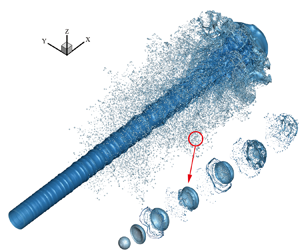
Figure 13. Phase distribution and grids in simulation. The droplet is severely deformed and broken during the atomization, and the AMR technology refines the grid near the interface. The local zoom shows the mesh of the small droplets produced by the fragmentation.

4.1. Numerical results of primary breakup

In the DNS modelling of the primary breakup, the jet flow characteristics in a gas environment after leaving the nozzle are investigated without considering the flow behaviour inside the nozzle. In addition, the effect of gravity is ignored. The calculation domain is a cube with a side length of 5 mm, and the spray nozzle is located at the centre of left side of the domain with a diameter (d ₀) equal to 0.25 mm. The velocity inlet boundary condition ${U_l} = 60\;\textrm{m}\;{\textrm{s}^{ - 1}}$ is applied. To mimic the disturbance introduced by the flow inside the nozzle and accelerate the atomization, a time-varying disturbance with a small amplitude was added to the inlet velocity of the liquid jet (Zandian et al. Reference Zandian, Sirignano and Hussain2019)

(4.1)\begin{equation}{u_l}(t) = {U_l}\left[ {1 + \gamma \sum\limits_{i = 1}^5 {\sin \frac{{2{\rm \pi}{U_l}t}}{{\frac{{(i + 1)D}}{8}}}} } \right],\end{equation}

where $\gamma $ is the amplitude factor with the setting value of 0.2 %. The right side of the calculation domain is set as the free outflow boundary, and symmetry boundary conditions are applied to the other four sides. Liquid nitrogen (LN₂) is employed as the working liquid with a temperature equal to 97 K. Meanwhile, the initial surrounding gas is gaseous nitrogen (GN₂) with a temperature equal to 100 K. The main physical properties of the working fluids are shown in table 2. The adaptive mesh technology is used, and the minimum grid size length is 2.4 μm.

Table 2. Physical properties in the calculation $(p = 5.88 \times {10^5}\;\textrm{Pa)}$.

It is noted that, in the following work, unless otherwise specified, the dimensionless time $t^{\prime} = t/{t^\ast }$ is used. Here, ${t^\ast }$ is the characteristic time, which can be determined by ${t^\ast } = {L^\ast }/{U_0}$; ${L^\ast }$ is the characteristic length. Figure 14 shows the evolution of the surface profile and vortex structure (i.e. λ2 isosurface) of the jet. The unstable Kelvin–Helmholtz waves are found to form at the beginning. They are characterized by a small amplitude, axisymmetric shape near the nozzle and the corresponding vortex structure is ring shaped. The foremost segment of the jet forms a mushroom-shaped tip, and droplets and ligaments continuously fall off the rim of the tip. As the jet develops, the unstable waves continue to grow under the action of aerodynamics, gradually deforming with 3-D characteristics and eventually forming multiple lobes. The vortex structure near the surface also undergoes similar deformations. Holes began to appear in the lobes, and droplets and liquid filaments broke off from the rims. Because many liquid fragments surround the liquid core, the atomization cone can be clearly observed. At the same time, numerous complex vortices are formed among the liquid column, ligaments and droplets, further aggravating the deformation and fragmentation of the jet.

Figure 14. Evolution of jet morphology. The grey surface is the jet atomization morphology, and the blue surface is the vortex structure (λ2 isosurface) near the jet.

4.2. Effect of phase change on the primary breakup

The evolution of the jet in an environment with a large temperature range was simulated to extensively investigate the effect of phase change on the primary breakup. Different environmental superheat degrees $(\Delta {T_v} = {T_\infty } - {T_{sat}})$ with 500 K, 1000 K and 1500 K are employed. Figure 15 shows the jet surface evolution at $t^{\prime} = 5$ under different $\Delta {T_v}$. It reveals that all jets have sequential structures of ring-mounted K-H unstable waves, 3-D K-H lobes and tips in the axial direction away from the nozzle outlet, accompanied by massive droplets and ligaments tapered around the liquid core. However, the quantity of droplets upstream significantly decreases with the increase of $\Delta {T_v}$. This can be attributed to the fact that the droplets in this area are the first formed by the breakup of the tip, resulting in a longer thermal exposure in the environment. In the midstream of the jet, the quantity of droplets is also reduced to a certain extent, and the surface structure of the liquid core changes with the increase of $\Delta {T_v}$, as shown in the local zoom on the right. According to Shinjo & Umemura (Reference Shinjo and Umemura2010) and Zandian et al. (Reference Zandian, Sirignano and Hussain2019), the broken droplets hit the liquid core, and the vortex near the droplets acts on the jet surface. These are the main reasons for the breakup of the K-H lobe. Under the impact of numerous droplets and the complex vortices, the K-H lobe structure is destroyed, and the jet surface behaves irregularly during the simulation without phase change. With $\Delta {T_v} = 1500\;\textrm{K}$, the K-H waves appearing at a certain frequency can still be observed, and the break occurs at the rim of the lobe although the surface is not smooth. Similar behaviours can also be observed in the corresponding vortex, as shown in the green box in figure 16. In this area, the gas flows over the droplets and a stretched strip-shaped vortex forms. The vortex of the non-vaporizing jet is omnidirectional. However, it tends to be consistent under high-temperature conditions, and the number of strip-shaped vortex structures increases with the increase of $\Delta {T_v}$. Therefore, the flow field near the liquid core is relatively simple due to the reduction of droplets, which is also an important reason for the differences in the surface structures of the liquid core in figure 15.

Figure 15. Jet morphology under different environmental superheat conditions at $t^{\prime} = 5$. Images 1, 2 on the right are respectively local zoom of the jet surface with $\Delta {T_v} = 0$ and 1500 K. The cloud of tiny droplets near the jet has been deleted, and only the larger liquid structure is left.

Figure 16. Vortex behaviour under different environmental superheat conditions at $t^{\prime} = 5$. In the green box, the vapour flows over the droplets around the jet to form a large number of stretched strip-shaped vortex structures.

The average volume distributions of broken droplets with various $\Delta {T_v}$ are compared in figure 17, where the grey dashed line represents the corresponding minimum cell volume. With no phase-change condition $(\Delta {T_v} = 0)$, the droplet volume is normally distributed, and the mesh resolution can capture the droplets produced by the primary breakup. As $\Delta {T_v}$ increases, the volume distribution curve moves left, meaning that the quantity of large droplets decreases and the number of small droplets increases. This is mainly attributed to the reduction of the volume of all droplets caused by the occurrence of the phase change. The large droplets are highly unstable and prone to be deformed into liquid bags, sheets and ligaments. Take the sheet as an example, the air flows over the sheet to form a vortex, which will push the sheet to deform and thicken its rim. After breakup, the droplets formed by the rim are larger than those formed by the core. In a high-temperature environment, the vapour velocity near the rim is large, and the heat and mass transfers are more rapid. The sheet gets thinner and eventually breaks into smaller droplets. We discuss this in more detail in the section of secondary atomization this problem. Meanwhile, it seems that the total number of droplets also decreases. The curve of $\Delta {T_v}$ equal to 1500 K is steep on the left side of the minimum cell volume line because the grid resolution is not high enough to capture smaller droplets for this case. Considering that the variation trend of Sauter mean diameter (SMD) under phase change has been clarified and a finer grid will significantly increase the computational resource consumption, the current resolution is regarded as feasible for our requirements.

Figure 17. Droplet-volume distribution with no phase change and different superheat conditions at $t^{\prime} = 5.5$. The grey dashed line is the volume corresponding to the smallest cell. In simulations, it is generally believed that the dynamic behaviour of droplets cannot be accurately described at scales smaller than the minimum cell volume.

The droplet quantity distributions along the axial direction are further studied, as in figure 18. An obvious peak occurs on the curve without phase change at approximately x = 2, which does not appear on the curve with $\Delta {T_v} = 1500\;\textrm{K}$. In the middle and downstream, the deviation of the two curves becomes smaller, whereas the peak value of the curve with no phase change is slightly larger than the other. In general, the distribution curve at $\Delta {T_v}$ equal to 1500 K shows multiple peaks, indicating that the droplets fall off at a certain frequency. This is related to the K-H wave on the jet surface and the Rayleigh–Taylor (R-T) wave at the front end of the jet. When there is no phase change, the lobe structure is destroyed under the effect of a large number of droplets formed by breakage, as in figure 15 and the vortex in figure 16. It results in a variation in the droplet shedding frequency, and the curve only has peaks at the front and end. A detailed droplet-volume distribution at different locations along the axial direction is summarized in figure 19. It reveals that the case with no phase change presents normal droplet-volume distributions at different locations. In contrast, the peak of the droplet-volume distribution tends to move left close to the nozzle with $\Delta {T_v} = 1500\;\textrm{K}$. This is consistent with the phenomenon observed from the jet morphology in figure 15, indicating that phase change obviously affects the spatial and volume distribution of droplets.

Figure 18. Distribution of droplet quantity along the axial direction at $t^{\prime} = 5.5$. Here, x is a dimensionless parameter.

Figure 19. Axial volume distribution of droplets under different conditions at $t^{\prime} = 5.5$. According to the axial distance from the entrance x = 0–3.15, 3.15–4.0, 4.0–5.12 (dimensionless parameters), the jet is divided into upstream, middle and downstream, respectively. And the local droplet-volume distributions in each part are shown. (a) No phase change and (b) $\Delta {T_v} = 1500\;\textrm{K}$.

5.1. Droplet deformation and breakage without phase change

Compared with the primary breakup, the secondary atomization stage lasts longer; the movement morphology is more diverse, the coupling mechanism between phase change and droplet breakup is more complex. Hsiang & Faeth (Reference Hsiang and Faeth1995) divided the atomization and the droplet deformation into different modes according to the We and Oh (ratio of viscous force to surface tension) numbers of the droplet, including deformation, oscillation, bag breakup, etc. (shown in figure 20). According to the droplet-volume distribution obtained by the primary breakup simulation of the jet, a droplet diameter equal to the peak value of the distribution curve is taken as the initial value ${D_0} = 6\;{\rm \mu} \textrm{m}$ in the DNS of the droplet atomization. The main physical properties of the two phases are shown in table 2. The Oh number of the droplets is 0.0186 and the initial We numbers are set as 2.97, 9.63, 26.75, 74.3 and 199.85. As a result, the corresponding coordinate points are located in the five mode areas of deformation, oscillation deformation, bag breakup, multimode breakup and shear breakup mode in figure 20. The side length of the computational domain and the minimum cell size are set as 16.67D ₀ and 0.008D ₀, respectively. The surrounding boundary adopts the symmetry, and the top and bottom boundaries impose the outflow boundary condition. The numerical set-up is illustrated in detail in figure 21, and this flow-field set-up is used in all secondary atomization simulations in § 5.

Figure 20. The We–Oh diagram of the secondary atomization mode. In the grey area where Oh < 0.1, the secondary atomization mode is only determined by We.

Figure 21. Schematic sketch of a droplet moving in stationary vapour. The computational domain is a cube with a side length of 16.67D ₀. In the simulation, physical parameters are processed without dimension. At the initial moment, the droplet velocity along the y-axis is −1 and the vapour velocity is zero. Setting the symmetry boundary conditions around the calculation domain (light blue filled), and the top and bottom surfaces as the outflow boundary (light green filled).

The morphology evolutions of droplet motion with various initial We numbers are shown in figure 22. It reveals that the droplets only experience elastic deformation without breakage during the whole process at small We, as shown in figures 22(a) and 22(b). As We increases, the droplet deformation amplitude increases and the morphological variation becomes more diverse. At large We numbers, as shown in figure 22(c–e), the large aerodynamic force against the surface tension means that the droplets are unable to rebound under the action of surface tension, leading to breakage. A typical bag break can be observed in figure 22(c). The bottom of the bag was first torn into a net shape and then broken into smaller droplets. Subsequently, an obvious Rayleigh–Plateau instability was formed on the rim, resulting in the generation of larger droplets. In the case shown in figure 22(d), the rim of the bag is continuously stretched and contracted inward to form a neck. The breakage first appears on the neck, followed by the bag core. The evolution of such a droplet morphology is very similar to the double-bag breakup observed by Cao et al. (Reference Cao, Sun, Li, Liu and Yu2007) in their experiment. As We further increases in figure 22(e), the droplet deforms into a flat liquid sheet instead of a hemispherical bag. Droplets and ligaments are continuously broken off on the rim until the liquid sheet is completely fragmented. It is noted that a large We also leads to a more violent droplet breakage with a shorter breaking time and smaller droplet size. As We increases, the droplet atomization modes in figure 22 are successively deformation, oscillation deformation, bag breakup, multimode breakup and shear breakup. It can be concluded that our simulation results are completely consistent with the predictions in the secondary atomization mode diagram from Hsiang & Faeth (Reference Hsiang and Faeth1995) (figure 20). The simulation results are further compared with the experimental results by Dai & Faeth (Reference Dai and Faeth2001). Dai & Faeth (Reference Dai and Faeth2001) experimentally tested the secondary atomization of droplets in the range of 20 < We < 81. The evolutions of the dimensionless maximum diameters obtained by experiments and simulations are compared in figure 23, which indicates that the numerical results with We equal to 26.75 and 74.03 show satisfactory coincidence with the experimental results.

Figure 22. Deformation and fragmentation processes of droplets with different We. Here, $t^{\prime}$ is dimensionless time $t^{\prime} = t{U_0}/L$. Note that ${U_0}$ is the droplet initial velocity, which is different in these five cases. Therefore, the corresponding dimensionless time scales are also different.

Figure 23. Variation in the maximum diameter of a droplet with time. Here, ${D_{max}}$ is the maximum diameter of the droplet along the cross-stream, and the characteristic time ${t_c} = {D_0}{({\rho _l}/{\rho _g})^{1/2}}/{U_0}$.

5.2. Breakup performance of vaporizing droplets at high We

As mentioned above, the ISM is suitable for the violent breaking process of high We droplets. Assuming that the initial droplet is saturated, the initial environment temperature and the surrounding boundary temperature are kept consistent and Dirichlet boundary conditions are imposed at the gas–liquid interface ${T_\varGamma } = {T_{sat}}$ and computational domain boundary ${T_w} = {T_v}$.

The morphological evolution of droplet atomization with We = 199.85 and $\Delta {T_v} = 0\;\textrm{K},\;500\;\textrm{K}$ is shown in figure 24. Similar to the no phase-change case as in figure 24(a), droplet atomization stages from drop deformation, rim strip, neck breakup to sheet breakup are observed at $\Delta {T_v} = 500\;\textrm{K}$, as shown in figure 24(b). No droplets are generated during the deformation stage, and then droplets begin to fall off the rim of the droplets under the action of aerodynamic shear. At the same time, the rim shrinks to the inner centre, forming a neck due to the effect of surface tension. The joint between the neck and the liquid sheet has the largest surface curvature, and holes appear here and the neck separates from the liquid sheet. Finally, the sheet continues to stretch and lose stability, and holes begin to appear. With the effect of the capillary force, they develop along the radial direction and coalesce with other holes, making the liquid sheet appear to be broken into a network.

Figure 24. Morphology evolution of drop atomization. The typical characteristics of the droplet morphology development of We = 199.85 at several moments with $\Delta {T_v} = 0,\;500\;\textrm{K}$ are shown in (a,b).

However, the details of the broken form are different from those of the no phase-change case. It can be seen from the droplet shape in figure 24(a) that the bottom of the liquid sheet is first broken under the impact of the tiny droplets, and breakup begins to spread to the surrounding rim. In contrast, the bottom and rim around break almost at the same time when phase change exists, as shown in figure 24(b) at $t^{\prime} = 6$. The liquid being more evenly distributed in the core of the liquid sheet explains this phenomenon. Moreover, the results obtained after the completion of atomization at $t^{\prime} = 7$ also indicate that the droplet atomization is more violent with $\Delta {T_v} = 500\;\textrm{K}$.

To gain more insight, figure 25 shows the temperature and relative velocity distribution in the 2-D cross-section of the droplet at $t^{\prime} = 5$. It is found that the gas temperature at the rear of the droplet is unevenly distributed. At the same time, a symmetrical vortex pair is formed by the airflow at the rear of droplet, as shown in figure 25(b). Recirculation by the vortex enhances the gas convection inside the droplet rim. As a result, phase change accelerates at the inner side of the edge, which quickly vaporizes the liquid accumulated here. It can be concluded that phase change changes the liquid distribution inside the sheet to a certain extent, also accounting for the difference in droplet atomization morphology.

Figure 25. (a) Temperature field near the droplet of case We = 199.85, $\Delta {T_v} = 500\;\textrm{K}$, at $t^{\prime} = 5$. The black solid line is the gas–liquid interface. The temperature is a dimensionless parameter processed by $(T - {T_s})/({T_v} - {T_s})$. (b) Relative velocity distribution and streamline diagram. Here, $ud_{y}$ is dimensionless velocity along the flow direction $ud_{y} = {U^{\prime}_y} - {U^{\prime}_{y,stag}}$, where ${U^{\prime}_{y,stag}}$ is the velocity at the stagnation point below the droplet.

The growth of the total number of droplets during atomization is plotted in figure 26. For most of the time during breakup, the counts of droplets without phase change is slightly higher than those with phase change. This is because extremely small droplets vaporize rapidly under high-temperature conditions. In addition, the three curves of the droplet count also shows a similar regularity, which reflects the development of morphology. Taking the case of no phase change as an example, the growth curve is divided into four stages according to the slope, as shown in figure 26. In the rim strip and neck breakup stages, droplet shedding in a high-temperature environment lags behind the condition of no phase change. In the process of droplet deformation, the recirculating airflow on the back causes the liquid to accumulate at the rim. As the rim becomes thicker, the edge separates from the sheet, forming ligaments with the effect of capillary instability. Under the phase-change conditions, the vapour flow velocity inside and outside the rim is the largest, as shown in figure 25(b). This phenomenon strengthens the heat and mass transfer here and alleviates the accumulation of liquid. Finally, in the sheet breakup stage, the droplet number increase is significantly faster than that without phase change. At $\Delta {T_v} = 250\;\textrm{K}$, phase change makes the sheet stretch more uniformly and break more completely, leading to droplet counts higher than the result without phase change. But the effect of violent vaporization prevails as $\Delta {T_v}$ increases to 500 K, and the final droplet counts decrease instead.

Figure 26. Counts of droplet changes during secondary atomization for different superheat conditions with We = 199.85. According to the slope, the blue lines, arrows and text divide the four stages of the no phase-change case, corresponding to the droplet-breakup stages including deformation, rim strip, neck breakup and sheet breakup. The other two curves can also be divided like this.

Figure 27 shows the corresponding volume distribution of atomized droplets with various gas superheats. Two peaks appear on the droplet-size distribution curve without phase change, and the right peak gradually disappears on the curves as $\Delta {T_v}$ grows. This is probably due to the thicker rim of the liquid sheet. The breakup of the rim lags behind the breakage of the liquid sheet, and the size of the droplets produced is slightly larger. However, the occurrence of phase change improves this phenomenon by making the liquid distribution inside the liquid sheet uniform and reducing the volume of the large droplet. Moreover, the droplet-volume distribution peak shifts to the left as the environmental superheat increases; the droplet size is concentrated at the corresponding volume of the minimum cell. The main reasons are that the phase change reduces the volume of all droplets, and the fragmentation of the liquid sheet produces more droplets with smaller volumes.

Figure 27. Volume distribution of atomized droplets of We = 199 under different superheat conditions at $t^{\prime} = 8$. The grey dashed line is the volume corresponding to the smallest cell.

5.3. Breakup performance of the moving vaporizing droplets at low We

The DNS modelling of the droplet deformation with small We is carried out with STDM. The numerical set-up is the same as §§ 5.1 and 5.2. Figure 28 shows the movement and deformation of the droplet with $\Delta {T_v}$ and We equal to 500 K and 9.63, respectively. It reveals that the droplet deformation behaviour at some stages shows a significant difference from the case without phase change in figure 28(a). For example, the front edge of the droplet is almost flat at $t^{\prime} = 4$ in figure 28(b) and it is disc shaped in figure 28(a) without phase change. Afterward, the droplet rebounds and bulges upward and becomes a semi-ellipse at $t^{\prime} = 6$, instead of a flying-saucer shape as in figure 28(a).

Figure 28. Droplet morphology evolution of We = 9.63. (a) Without phase change. (b) With the condition of $\Delta {T_v} = 500\;\textrm{K}$. Figure shows the dimensionless temperature contour at different moments. The symmetrical vortex pair caused by recirculation can be observed.

To clarify the reason for the abovementioned difference, the drag coefficient is employed to analyse gas flow resistance against the droplet. The unsteady drag coefficient (Shao et al. Reference Shao, Luo and Fan2017) (5.1) is calculated from the deformation and velocity variation of the droplet

(5.1)\begin{equation}{C_D} = \frac{{{\rho _l}V\frac{{\textrm{d}{U_r}}}{{\textrm{d}t}}}}{{\frac{1}{2}{\rho _v}U_r^2{A_{front}}}},\end{equation}

where V and ${A_{front}}$ are the liquid volume and frontal area, respectively; ${A_{front}}$ can be obtained from ${A_{front\; }} = {\rm \pi}{({D_{max}}/2)^2}$; ${U_r}$ is the relative velocity and defined as ${U_r} = {U_l} - {U_v}$.

The variation trend of Re and We during the movement of the droplet is shown in figure 29. Under the effect of aerodynamic resistance, both Re and We related to the velocity gradually decrease and fluctuate with the deformation of the droplet. With the increase of environmental superheat, the droplet deceleration effect becomes more obvious. The decrease in the inertial force introduced by deceleration means that the surface tension gradually dominates the deformation. The droplet rebounds quickly once it deviates from the equilibrium state, which explains that the droplet's deformation amplitude decreases with the increase of temperature. Consequently, the variation of ${C_D}$ can be obtained according to (5.1) with various $\Delta {T_v}$, as in figure 30. This illustrates that ${C_D}$ rapidly decreases initially when Re decreases, which is attributed to the impulsive acceleration of droplet in a stationary gas reported by Wadhwa, Magi & Abraham (Reference Wadhwa, Magi and Abraham2007). Then, ${C_D}$ experiences a slow decrease stage as Re gradually decreases. Obvious fluctuations appear at Re approximately equal to 600. This is related to the deformation of the droplet and the fluctuation of the droplet acceleration. Besides, ${C_D}$ increases with the growth of $\Delta {T_v}$, indicating that the droplet suffers more aerodynamic resistance when travelling in a higher-temperature environment.

Figure 29. Variation trends of Re and We during droplet movement. The y-axis on the left is Re, and the right is We. The solid red line and the coloured hollow dots represent the changes of Re over the dimensionless time under different superheat conditions. The green solid line and the coloured solid dots represent the variation in We.

Figure 30. Variation in ${C_D}$ during droplet movement under different superheat conditions. Here, Re will gradually decrease as the droplet advances. Therefore, curves from right to left in the figure are the evolution of ${C_D}$ during the droplet movement.

When the gas–liquid interface undergoes phase change, a typical flow feature is the velocity jump across the interface along the normal direction, which is produced by the volume expansion in the gas phase, also known as Stefan flow. The streamline diagrams of the droplets without and with phase change are depicted in figures 31(a) and 31(b), respectively. The stagnation point below the droplet is taken as the reference system. The streamlines closely adhere to the surface of the droplet and flow around without phase change, as shown in the red circle in figure 31(a). In contrast, the gas streamlines nearly below the droplet do not adjoin the interface in figure 31(b). The streamline that goes from the droplet surface into the vapour indicates the appearance of Stefan flow. Consequently, the near region of the interface can be treated as a vapour interlayer. Figure 31(c) shows the temperature distribution (in the form of isolines) and the mass source term distribution (in the form of contours) near the vaporizing droplet. The temperature boundary layer is thinner upwind of the droplet, resulting in a significantly larger temperature gradient than at other positions, and thus a larger corresponding mass source term. It can be understood that the heat and mass transfers on the droplet surface are not uniform during the movement, and they impact the velocity field in the form of Stefan flow in reverse. The difference in vapour velocity above and below the droplet provides a buffer for the movement of the droplets, which is an important reason for the increase of the aerodynamic resistance on the droplet (described by the drag coefficient) and the subsequent decrease of droplet deformation.

Figure 31. (a) Streamline diagram at $t^{\prime} = 0.5$ without phase change. The solid blue line is the gas–liquid interface. The streamlines of the vapour below the droplet are shown by the red circle. (b) Streamline diagram at $t^{\prime} = 0.5$ with $\mathrm{\Delta }{T_v} = 500\;\textrm{K}$. (c) Temperature and mass source term distribution near the droplet with $\mathrm{\Delta }{T_v} = 500\;\textrm{K}$ at $t^{\prime} = 0.5$. The coloured line represents the temperature isolines, and the fill colour represents the contour of the mass source term.

5.4. Phase-change rate for various We

Phase-change rates for various We are further investigated. The variation of the droplet equivalent diameter converted from the remaining volume of the droplet is plotted in figure 32. The characteristic time ${t^\ast }$ in figure 32 is unified as ${t^\ast } = {L^\ast }/{U_0}$, where ${U_0}\; $is equal to $10\;\textrm{m}\;{\textrm{s}^{ - 1}}$. With the increase of We, the equivalent droplet diameter decreases with acceleration. A local zoom of the beginning of the cases with large We reveals that the two curves experience slow followed by fast variation.

Figure 32. Variation of droplet equivalent diameter with dimensionless time at $\mathrm{\Delta }{T_v} = 500\;\textrm{K}$ of different We. Considering that the time scales of several cases are significantly different, two large We cases are shown independently.

Accordingly, phase-change rates can be obtained from the variation of the droplet equivalent diameter as in figure 33. It is seen that the phase-change rate significantly increases with the increase of We. Moreover, curves are varied smoothly with small We. The occurrence of deceleration and deformation is attributed to the curve variation. Once droplet breakup happens (We = 74.3 and 199.85), the phase-change rate varies drastically.

Figure 33. Variation of droplet-volume phase-change rates with dimensionless time at $\mathrm{\Delta }{T_v} = 500\;\textrm{K}$ for different We. The discretized phase-change rate can be calculated by $(V_d^{n + 1} - V_d^n)/\Delta t$, where ${V_d}$ is the remaining volume of the droplet.