3.1. Kinetic energy term

By definition, the kinetic energy of deformation of the droplet is

(3.3)\begin{equation} T_L = \tfrac{1 }{2}\rho _L {\iiint}_{{V( t )}} {{\boldsymbol{V}}^{{2}}\, \textrm{d}^3 x}, \end{equation}

where $V(t)$ is the volume occupied by the droplet. This integral can be computed once the velocity field is known. Using (3.2), one gets, for the oblate case,

(3.4)\begin{equation} T_L = \frac{1 }{2}\rho _L \left( {\frac{{\dot y} }{y}} \right)^2 \iint_{Ellipse(yR_0 ,R_0 /y^2 )} {( {r^2 + 4z^2 } )2{\rm \pi} r\, \textrm{d} r\, \textrm{d} z} = \frac{2 }{3}{\rm \pi}\rho _L R_0^5 K_C ( y )\left( {\frac{{\dot y} }{y}} \right)^2 , \end{equation}

where the non-dimensional term $K_C$ should be of order unity. This leads to

(3.5)\begin{equation} K_C^O( y ) = \frac{4}{5}\frac{{2 + {y^6}}}{{{y^4}}}, \end{equation}

where the superscript letter $O$ indicates oblate deformation. However, in order to later develop a simplified model, it will be more convenient to develop $K_C$ around the spherical shape using the new deformation parameter $\varepsilon = y-1 \ll 1$,

(3.6)\begin{equation} \tilde K_C^O( \varepsilon ) = K_C^O( {1 + \varepsilon } ) = \tfrac{{12}}{5} - \tfrac{{24}}{5}\varepsilon + \tfrac{{84}}{5}{\varepsilon^2} + O( {{\varepsilon ^3}} ), \end{equation}

where the notation $\tilde {K}(\varepsilon )=K(y)$ has been used. Relevance of this linearisation (when restricted to first order) will be discussed throughout the text. In the case of deformation into a prolate spheroid ($\varepsilon <0$), one gets

(3.7)\begin{equation} K_C^P( y ) = \frac{4}{5}\frac{{1 + 2{y^{12}}}}{{{y^4}}}, \end{equation}

where the superscript $P$ indicates prolate deformation and

(3.8)\begin{equation} \tilde K_C^P( \varepsilon ) = K_C^P( {1 + \varepsilon } ) = \tfrac{{12}}{5} + \tfrac{{48}}{5}\varepsilon + \tfrac{{264}}{5}{\varepsilon^2} + O( {{\varepsilon ^3}} ). \end{equation}

Note that $K_C(1)=\tilde {K}_C(0) = 2.4$ in both cases and is of order unity. Note also that, while $K_C$ is continuous in 1, its derivatives are not. Lastly, note that these values may be slightly underestimated for a droplet falling at terminal velocity since the inner vortices are not included.

3.2. Viscous dissipation term

Likewise, the viscous dissipation due to internal flow can be estimated through

(3.9)\begin{equation} D = \mu _L \int_V {\frac{{\partial V_i } }{{\partial x_j }}\frac{{\partial V_i } }{{\partial x_j }}}\, \textrm{d}^3 x. \end{equation}

In the case of a purely extensional flow, as given by (3.2), the computation leads to

(3.10)\begin{equation} D = \mu _L \iiint_{{S( y )}} {12\left( {\frac{{\dot y} }{y}} \right)^2 \, \textrm{d}^3 x} = 16{\rm \pi} R_0^3 \mu _L \left( {\frac{{\dot y} }{y}} \right)^2 . \end{equation}

This is exactly the result given by Schmehl (Reference Schmehl2002) and, similarly, only the value of the constant coefficient in (3.10) differs from the original DDB model.

3.3. Surface energy term

Surface of an oblate ellipsoid is given by the exact formula

(3.11)\begin{equation} S = 2{\rm \pi} a^2 + {\rm \pi}\frac{{b^2 } }{e} \log \left( {\frac{{1 + e} }{{1 - e}}} \right), \end{equation}

where eccentricity $e$ is given by

(3.12)\begin{equation} e = \sqrt {1 - \frac{{b^2 } }{{a^2 }}}. \end{equation}

Note that $e$ relates to the other deformation parameters as $e=\sqrt { 1- {1}/{y^6}} \approx \sqrt {6\varepsilon }$. Time variation of surface energy can now be expressed as

(3.13)\begin{equation} \frac{{\textrm{d} E_S } }{{\textrm{d} t}} = \sigma \frac{{\textrm{d} S } }{{\textrm{d} y}}\frac{{\textrm{d} y} }{{\textrm{d} t}} = \sigma 4{\rm \pi} R_0^2 K_S ( y ) \frac{{\dot y} }{y}. \end{equation}

When $1 < y$, the non-dimensional surface energy function $K_S$ is equal to

(3.14)\begin{equation} K_S^O( y ) = \frac{{2{y^5}\sqrt {\dfrac{{ - 1 + {y^6}}}{{{y^4}}}} ( {1 + 2{y^6}} ) + ( {1 - 4{y^6}} )\log \left[ { - 1 + 2{y^5}\left( {y + \sqrt {\dfrac{{ - 1 + {y^6}}}{{{y^4}}}} } \right)} \right]}}{{4{y^7}{{\left( {\dfrac{{ - 1 + {y^6}}}{{{y^4}}}} \right)}^{3/2}}}}, \end{equation}

and can be approximated by

(3.15)\begin{equation} \tilde K_S^O( \varepsilon ) = K_S^O( {1 + \varepsilon } ) = 0 + \tfrac{{16}}{5}\varepsilon + \tfrac{{24}}{{35}}{\varepsilon^2} + O( {{\varepsilon^3}} ). \end{equation}

Likewise, considering that the formula for the surface of a prolate spheroid is

(3.16)\begin{equation} S = 2{\rm \pi} {a^2}\left( {1 + \frac{b}{{ae}}\arcsin e} \right), \end{equation}

this leads to the exact formula

(3.17)\begin{equation} K_S^P( y ) = - \frac{{{y^3}\sqrt {1 - {y^6}} ( {1 + 2{y^6}} ) + ( {1 - 4{y^6}} )\arccos [ {{y^3}} ]}}{{2y{{( {1 - {y^6}} )}^{3/2}}}}. \end{equation}

One gets as an approximation, when $\varepsilon < 0$,

(3.18)\begin{equation} \tilde K_S^P( \varepsilon ) = K_S^P( {1 + \varepsilon } ) = 0 + \tfrac{{16}}{5}\varepsilon + \tfrac{{24}}{{35}}{\varepsilon^2} + O( {{\varepsilon^3}} ). \end{equation}

Note that $K_S$ is negative in the prolate case ($\varepsilon < 0$), as when $y$ decreases i.e. $\dot {y}<0$, the surface energy should still increase over time (i.e. the product $K_S \dot {y} > 0$), as the sphere is the volume of minimal surface. Note also that the identity of developments (3.15) and (3.18) shows that the coefficient $K_S$ is at least $C^2$ smooth around the spherical shape.

3.4. Carrier fluid pressure term

Carrier fluid pressure term is actually the gist of the present droplet oscillator model. When a droplet oscillates, deforms and eventually breaks up in an exterior flow field, the Reynolds number is usually not small and it is therefore possible to make the assumption that the carrier fluid flow around the drop is a potential flow. Classical analytical results for potential flow around a spheroid can therefore be used (Lamb Reference Lamb1932; Milne-Thomson Reference Milne-Thomson1968). This is not a new idea, as the possibility for the flow to be potential on the upwind side of a falling droplet has been emphasised for some time (cf. Fuchs (Reference Fuchs1964) for instance). However, on the downwind side, flow separation is to be expected; therefore, two hypotheses will be developed hereafter: one will assume that the pressure works symmetrically on the two sides of the droplet ($C_P=1$) whereas the second will assume that the pressure only works on the forward half of the droplet ($C_P=1/2$).

Using Stokes’ axisymmetric streamfunction $\psi$, the velocity field can be computed with

(3.19a,b)\begin{equation} U_{{z}} = \frac{{ - 1}}{r}\frac{{\partial \psi }}{{\partial r}} \quad \textrm{and} \quad U_{{r}} = \frac{1}{r}\frac{{\partial \psi }}{{\partial z}}, \end{equation}

and the streamfunction $\psi$ is given, in the droplet frame of reference, by

(3.20)\begin{align} \psi &= \frac{{ - \frac12 U_\infty ( {a^2 - b^2 } )} }{{e\sqrt {1 - e^2 } - \textrm{Sin}^{ - 1} ( e )}}( \textrm{Sinh} ( \xi ) - \textrm{Cosh}^2 ( \xi )\textrm{Cot}^{-1} ( \textrm{Sinh} (\xi)))\textrm{Sin}^2 ( \eta )\nonumber\\ &\quad - \frac{1}{2}U_\infty r( {\xi ,\eta } )^2 , \end{align}

where spheroidal coordinates $(\xi ,\eta )$ are obtained from the cylindrical coordinates $(r,z)$ through the conformal mapping

(3.21)\begin{equation} z + ir = \sqrt {a^2 - b^2 } \textrm{Sinh} ( {\xi + i\eta } ). \end{equation}

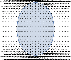
Note that (3.21) must be inverted (analytically) before using (3.19a,b) and (3.20). Figure 2 shows the resulting potential flow. Pressure power is then computed using (cf. appendix D for details of the approximation)

(3.22)\begin{equation} \dot{W}_P = - \mathop{{\int\!\!\!\!\!\int}\mkern-21mu \bigcirc}\limits_{\partial V} {P( {{\boldsymbol{V}}{\boldsymbol{\cdot} \boldsymbol{n}}} )\, \textrm{d} S} \approx 2\rho _C \int_0^a {\tfrac12 {\boldsymbol{U}}^2 ( {{\boldsymbol{V}}{\boldsymbol{\cdot} \boldsymbol{n}}} )2{\rm \pi} r\, \textrm{d} l(r)} , \end{equation}

where $\boldsymbol {n}$ is the outer normal to the spheroid and $\textrm {d} l(r)$ a small length increase along the ellipse generating the ellipsoid. Note that introducing Hill's vortex should not change this value as ${\boldsymbol {V}}_{Hill}\boldsymbol {\cdot } \boldsymbol {n} = 0$. Note also that $\dot {W}_P$ should be positive for the droplet to deform, (note also that this is one of the main differences from Schmehl (Reference Schmehl2002)). When the droplet deforms into a spheroid, this integral can be given the form

(3.23)\begin{equation} \dot{W}_P = \rho _C U_\infty^2 {\rm \pi}R_0^3 C_P K_P ( y ) \frac{{\dot y} }{y}, \end{equation}

where non-dimensional function $K_P$ is also expected to be of order unity; $C_P$ is a coefficient whose value equals either 1 or $1/2$, respectively, if the pressure work is computed on the whole droplet or only on the forward half of the droplet. Deriving a closed form for $K_P$ in (3.23) is a little tricky; therefore, as a first approach, a polynomial interpolation of the value of $K_P$ in the range $1< y < 3$ has been computed with $Mathematica$ (Wolfram Research, Inc 2014)

(3.24)\begin{equation} K_P^O( y ) \approx 0.171103 - 0.924041y + 1.21925{y^2} + 0.473157{y^3} + 0.263002{y^4}. \end{equation}

Although a way of computing the exact expression will be presented now, this polynomial approximation is naturally smooth when $y \to 1$, paradoxically this may not be the case (numerically) when using the exact expression, as there is a singularity in the conformal transformation (3.21) when $a \to b$. Therefore, the polynomial interpolation will be mainly used in the numerical solution of the oscillator equation.

Figure 2. Axisymmetric potential flow around an oblate spheroid. Inner deformation field corresponding to (3.2) is also illustrated. Velocity is computed using the formulas (3.19a,b), (3.20) and (3.21). Note that norm of the velocity vectors inside the droplet is arbitrary as it should be the result of the final oscillator equation.

As stated, it is possible to derive an analytical solution (cf. appendix E). The final result is

(3.25)\begin{equation} K_P^O( y ) = \frac{{6 - 6{y^6} + 2\sqrt {1 - \dfrac{1}{{{y^6}}}} {y^3}( {2 + {y^6}} )\textrm{Arcsec} [ {{y^3}} ]}}{{{{\left( {\sqrt {1 - \dfrac{1}{{{y^6}}}} - {y^3}\textrm{Arcsec} [ {{y^3}} ]}\right)}^2}}}, \end{equation}

which can be approximated by

(3.26)\begin{equation} \tilde K_P^O( \varepsilon ) = K_P^O( {1 + \varepsilon } ) = \tfrac{6}{5} + \tfrac{{684}}{{175}}\varepsilon + \tfrac{{3366}}{{875}}{\varepsilon^2} + O( {{\varepsilon ^3}} ). \end{equation}

For the prolate case ($y < 1$), (cf. appendix F) this equation reads

(3.27)\begin{equation} K_P^P( y ) = - \frac{{4{y^6}\sqrt {1 - {y^6}} \left( {6\sqrt {1 - {y^6}} + ( {2 + {y^6}} )\log \left[ { - \dfrac{{ - 2 + {y^6} + 2\sqrt {1 - {y^6}} }}{{{y^6}}}} \right]} \right)}}{{{{\left( {2\sqrt {1 - {y^6}} + {y^6}\log \left[ { - \dfrac{{ - 2 + {y^6} + 2\sqrt {1 - {y^6}} }}{{{y^6}}}} \right]} \right)}^2}}}, \end{equation}

which can be linearised into

(3.28)\begin{equation} \tilde K_P^P( \varepsilon ) = K_P^P( {1 + \varepsilon } ) = \tfrac{6}{5} + \tfrac{{684}}{{175}}\varepsilon + \tfrac{{3366}}{{875}}{\varepsilon^2} + O( {{\varepsilon ^3}} ). \end{equation}

Note that, again, the identity of developments (3.26) and (3.28) shows that the coefficient $K_P$ is at least $C^2$ smooth around the spherical shape.

4.1. Nonlinear ordinary differential equation

The final equation is obtained by combining (3.1), (3.4), (3.10), (3.13) with (3.23). Using the Weber and Ohnesorge numbers as dimensional numbers, one gets the following oscillator equation:

(4.1)\begin{equation} \frac{\textrm{d}}{{\textrm{d}{t^*}}}\left( {{{\left( {\frac{{\dot y}}{y}} \right)}^2}{K_C}( y )} \right) + \frac{{96Oh}}{{\sqrt {We} }}{\left( {\frac{{\dot y}}{y}} \right)^2} + \frac{{48}}{{We}}{K_S}( y )\left( {\frac{{\dot y}}{y}} \right) = 6{K_P}( y )\left( {\frac{{\dot y}}{y}} \right), \end{equation}

where the non-dimensional time $t^*$ and the Ohnesorge number read

(4.2)\begin{gather} t^* = \frac{t}{\tau }, \end{gather}

(4.3)\begin{gather}Oh = \frac{{\mu _L }}{{\sqrt {\sigma \rho _L 2R_0 } }}, \end{gather}

and $We$ is the parameter that has been introduced in (2.8). In the following, this equation will be solved using $Mathematica$ (Wolfram Research, Inc 2014) and the stability of the steady state or of the initial spherical state will be studied.

4.2. Steady state computation

Steady state of the oscillator is given by the implicit relation

(4.4)\begin{equation} We = \frac{{8K_S ( y )} }{{K_P ( y )}}. \end{equation}

This leads to a formula identical to El Sawi's (Reference El Sawi1974) result for bubbles (note that this can be applied to the present case even when condition (2.16) is not met since El Sawi's work on ellipsoidal bubble deformation is about the steady state) and given by

(4.5)\begin{align} &We_{{El\ Sawi}}( y ) \nonumber\\ &\quad = \frac{{2{{( {\sqrt { - 1 + {y^6}} - {y^6}\textrm{Arcsec} [ {{y^3}} ]} )}^2}\left( {{y^3}\sqrt { - 1 + {y^6}} ( {1 + 2{y^6}} ) + ( {1 - 4{y^6}} )\textrm{Arctanh} \left[ {\dfrac{{\sqrt {- 1 + {y^6}} }}{{{y^3}}}} \right]} \right)}}{{{y^7}{{( { - 1 + {y^6}} )}^2}( { - 3\sqrt { - 1 + {y^6}} + ( {2 + {y^6}})\textrm{Arcsec} [ {{y^3}} ]} )}}. \end{align}

Figure 3 shows the graph of (4.4) for the oblate case (as in § 2 the prolate case has no steady solution as $K_S$ is negative while $K_P$ is positive). As pointed out by El Sawi (Reference El Sawi1974), there is no longer an oblate steady state for a Weber number greater than 3.27 (there also seems to be a branch for very large $y$ but it does not seem very likely to have any physical reality). For the sake of completeness, this result is compared to Moore's (Reference Moore1965) formula resulting from a two-point analysis based on potential flow around a spheroid

(4.6)\begin{equation} We_{Moore}( y ) = \frac{{4( {{y^9} + {y^3} - 2} )}}{{{y^4}{{( {{y^6} - 1} )}^3}}}{( {{y^6}\textrm{Arcsec} {(y^3)} - \sqrt {{y^6} - 1} } )^2}. \end{equation}

Note that combining (2.9) and (4.6) allows for the computation of function $\lambda$. Moore's result is still widely used in the analysis of bubble shape (Legendre, Zenit & Velez-Cordero Reference Legendre, Zenit and Velez-Cordero2012). The reader can see in this latter work that, while it is dedicated to developing new correlations, the shapes of bubbles are still well described by Moore's formula up to a Weber number approximately equal to 3.

Figure 3. Steady deformation for a liquid droplet in an exterior flow field. Continuous line is the solution of the analytical model given by (4.4) while the dotted line is the solution of the linearised (5.8).

There are, however, fewer comparisons in the liquid–liquid or the liquid–droplet/gas case and it will be shown here that the present result compares rather well with the data given in Hsiang & Faeth (Reference Hsiang and Faeth1995). Agreement between (4.4) and droplet/gas experiments in shock tubes (labelled by stars in figure 3) is rather good when $We < 3$. For liquid/liquid experiments agreement is also rather good for the lower Weber number ($We <1$) but there seems to be a tendency for intermediate Weber numbers ($1< We <4$) to follow an equilibrium shape given by twice the result of (4.4) and corresponding to the computation of the pressure work on the forward half of the droplet (i.e. $C_P=1/2$ corresponding to the dotted line in figure 3). Note that in the liquid–liquid case, it is likely that measurements have been made close to the limit falling velocity (this is not detailed, however, by Hsiang & Faeth Reference Hsiang and Faeth1995). Note also that the Taylor Analogy Breakup (TAB) model gives good values for the steady deformation when compared with gas-liquid cases (cf. appendix A.1).

4.3. Phase space analysis

Figure 4(a) shows the oscillatory behaviour for both initially oblate and prolate spheroids for $We = 2$ and $Oh = 0.001$. Note that, in most works, the initial shape is assumed to be spherical but it may actually depend on the experimental protocol devised (for instance a levitated droplet impinged by a horizontal shock or air blow might be slightly oblate but hit on the greater semi-axis; or a pendant drop detaching and hitting a liquid pool might still begin slightly prolate when it hits the surface). Figure 4(b) shows the phase plot for the previous oscillations. The fixed point is clearly visible as the centre of the circling motion (and is an attractor). Note that when the droplet begins in the prolate shape, this is equivalent to (i.e. it follows part of the same trajectory as) the oscillation of a spherical droplet with a non-zero initial deformation velocity, as there is some stored surface energy in the deformed droplet. This explains why the amplitudes of the oscillations are larger when the droplet begins in the prolate shape. Most experimental interpretations begin with a perfectly round droplet and a zero initial deformation velocity, however.

Figure 4. Comparison between oscillation time series and phase plot. (a) Oscillations, $\ We = 2, Oh = 0.001$; and (b) phase plot, $We = 2, Oh = 0.001$.

5.1. Stability of the steady states

From a mathematical point of view, studying the stability of a fixed point should be done by linearising around said fixed points, i.e. those obtained by (4.4) (this is also known as Lyapunov's first method). Setting $y_{eq}$ as the implicit solution of (4.4) and writing $\epsilon =y-y_{eq}$, one gets

(5.1)\begin{equation} {K_C}( {{y_{eq}}( {We} )} )\ddot \epsilon + \frac{{48Oh}}{{\sqrt {We} }}\dot \epsilon + \left( {\frac{{24}}{{We}}{\sigma _1}( {{y_{eq}}( {We} )} ) - 3{{\rm \pi} _1}( {{y_{eq}}( {We} )} )} \right)\epsilon = 0, \end{equation}

where

(5.2)\begin{gather} { K_S}( \epsilon ) \approx \sigma _0 + \sigma _1\epsilon + \sigma _2{\epsilon^2}, \end{gather}

(5.3)\begin{gather}{ K_P}( \epsilon ) \approx {\rm \pi}_0 + {\rm \pi}_1\epsilon + {\rm \pi}_2{\epsilon^2}. \end{gather}

In this new analysis, only values of the coefficients $\tilde {K}_C, \sigma _1, {\rm \pi}_1$ vary and they are now functions of the steady deformation $y_{eq}$ and henceforth of the Weber number (these relations are given by polynomial approximations in appendix G).

5.2. Stability of the initial spherical state

Although not very rigorous mathematically speaking, it is possible, however, to linearise equation (4.1) around $y=1$, using the previous definition $\varepsilon = y-1$; this leads to

(5.4)\begin{equation} {K_C}( 1 )\ddot \varepsilon + \frac{{48Oh}}{{\sqrt {We} }}\dot \varepsilon + \left( {\frac{{24}}{{We}}{{\tilde K}_S}( \varepsilon ) - 3{{\tilde K}_P}( \varepsilon )} \right) = 0. \end{equation}

Therefore, keeping the same notation as in (5.2) and (5.3), one gets

(5.5)\begin{equation} \ddot \varepsilon + \frac{{48Oh}}{{{K_C}( 1 )\sqrt {We} }}\dot \varepsilon + \frac{1}{{{K_C}( 1 )}}\left( {\frac{{24}}{{We}}{\sigma _1} - 3{{\rm \pi} _1}} \right)\varepsilon = \frac{1}{{{K_C}( 1 )}}\left( { - \frac{{24}}{{We}}{\sigma _0} + 3{{\rm \pi} _0}} \right), \end{equation}

and, using exact values of the coefficients found in (3.15), (3.18), (3.26) and (3.28) this leads to

(5.6)\begin{equation} \ddot \varepsilon + \frac{{20Oh}}{{\sqrt {We} }}\dot \varepsilon + \left( {\frac{{32}}{{We}} - \frac{{342}}{{35}}} \right)\varepsilon = \frac{3}{2}. \end{equation}

It can be noticed that the final results is very close to Reference Kulkarni and SojkaKulkarni & Sojka's (Reference Kulkarni and Sojka2014) model given by

(5.7)\begin{equation} \ddot y + \frac{{16Oh}}{{\sqrt {We} }}\frac{1}{{{y^2}}}\dot y + \left( {\frac{{24}}{{We}} - \frac{{{\alpha^2}}}{4}} \right)y = 0. \end{equation}

Note that in (5.7), the value of the damping coefficient has been set to 16 instead of 8, as in the original work, as there seems to be a mistake in their derivation. The coefficient $\alpha$ is a fitting coefficient that is based, according to the authors, on the stretching rate of the air around the droplet and considering § 2, it corresponds to $\alpha =2\lambda$. Therefore, it should be greater than 3 (twice the spherical droplet case). However, Kulkarni and Sojka decided to set it equal to $2\sqrt {2}$ in order to recover the classical value of the critical Weber number, usually set to 12 (q.v.). Note that there is no right-hand term in their model, so that, rigorously, the equilibrium shape should be given by $y=0$ (i.e. a zero width) which is somewhat non-physical. The right-hand term in (5.5) does, however, lead to steady deformations $\bar \varepsilon$. They can be easily computed and this leads to

(5.8)\begin{equation} \bar \varepsilon = \frac{{( {{{{{\rm \pi} _0}}/{{{\rm \pi} _1}}}} )We}}{{W{e_{cr}} - We}} \simeq \frac{{0.3We}}{{W{e_{cr}} - We}}. \end{equation}

Here, $We_{cr}$ is a critical Weber number which reads

(5.9)\begin{equation} W{e_{cr}} = \frac{{8{\sigma _1}}}{{{{\rm \pi} _1}}}. \end{equation}

In the case of linearisation around the sphere with $C_P=1$, in (5.9) we get $We_{cr}= ( {{1120}}/{{171}}) \simeq 6.54$ (and $C_P=1/2$ leads to $We_{cr}=13.08$). Figure 3 compares the steady deformation obtained by (4.4) (full nonlinear model) and (5.8) (linearised) and the two seem to be in agreement up to a Weber number of 2.4.

5.2.1. Linear stability

Stability of either (5.1), (5.5) or (5.7) can be obtained using the discriminant which reads

(5.10)\begin{equation} \varDelta = {\alpha^2}\left( {\left( {\frac{{W{e_{cr}}}}{{We}}} \right)\left( {{{\left( {\frac{{Oh}}{{O{h_{cr}}}}} \right)}^2} - 1} \right) + 1} \right), \end{equation}

after introducing

(5.11)\begin{equation} \alpha = \sqrt {\frac{{12{{\rm \pi} _1}}}{K_{C(1)}}}, \end{equation}

($\alpha =4.42$ when $C_P=1$ and $\alpha =3.12$ when $C_P=1/2$) and the critical Ohnesorge number $Oh_{cr}$ defined by

(5.12)\begin{equation} Oh_{cr} = \sqrt {\frac{{K_{C(1)} \sigma _1 } }{{24 }}}. \end{equation}

In the case of linearisation around the sphere with $C_P=1$, $Oh_{cr} \simeq 0.54$, the condition for oscillation, $\varDelta < 0$, sums up to

(5.13)\begin{equation} Oh^2 < (Oh_{cr})^2 \left( {1 -\frac{{We }}{{We_{cr} }}} \right). \end{equation}

This limits the oblate oscillation zone (cf. figure 5). For the model given by (5.1), $Oh_{cr}$ is a function of $We$: this is referred as the ‘Analytical’ model in figure 5. Note that Reference Kulkarni and SojkaKulkarni & Sojka's (Reference Kulkarni and Sojka2014) model corresponds to $\alpha ^2= 8, We_{cr}=12$ and $Oh_{cr}=1.63$. They, however, did not compute $Oh_{cr}$ or its equivalent as they wrongly computed the oscillation domain. Note also, and more importantly, that the real parts of the roots of the characteristic equation are positive when $We > We_{cr}$ leading to a possible droplet blow-up. There is also an area of critical damping of oscillation when $We < We_{cr}$ and Ohnesorge number is large enough.

Figure 5. Stability of the droplet in the $We\hbox{--}Oh$ chart. Horizontal lines separate the stable and unstable domains. The domain of oscillations are computed using (5.13), (5.9), (5.12) and in the nonlinear cases, (G 3), (G 4) or (G 6), (G 7).

5.3. Oscillation frequency

The non-dimensional oscillation frequency is given by

(5.14)\begin{equation} f = \frac{\alpha}{{4{\rm \pi} }}{\left( {\left( {\frac{{W{e_{cr}}}}{{We}}} \right)\left( {1 - {{\left( {\frac{{Oh}}{{O{h_{cr}}}}} \right)}^2}} \right) - 1} \right)^{1/2}}. \end{equation}

Which in the linearised case around a sphere with $C_P=1$, leads to

(5.15)\begin{equation} f \simeq \left( {\frac{{0.81}}{{We }} - 0.12} \right)^{1/2}, \end{equation}

where influence of the Ohnesorge number has been neglected in the last equation (when $C_P=1/2$ this equation becomes $f=\sqrt {.81/We-0.06}$). Note that the Weber number dependency of the frequency is mainly coupled to the ratio between surface and kinetic energy of deformation (through (5.11), (5.9) and (5.14)). Therefore, discrepancies between these models and experiments can be somewhat related to the different hypotheses that are validated. For instance, increase of surface area (e.g. by non-spheroidal deformation) will increase the frequency while increase of the kinetic energy (by introducing, for instance, Hill's vortices) would decrease it. Next section will therefore test the different oscillation models against DNS and experiments.

5.3.1. Comparison with data

In figure 6 we show a comparison of the frequency predicted by the present model and previous ones. Lamb's result given by (5.16) gives much higher frequencies

(5.16)\begin{equation} {f_{Lamb}} = \frac{{1,27}}{{\sqrt {1 + \dfrac{2}{3}\dfrac{{{\rho _C}}}{{{\rho _L}}}} }}\frac{1}{{\sqrt {We} }}, \end{equation}

while Villermaux & Bossa's (Reference Villermaux and Bossa2009) model gives much lower frequencies. The TAB model gives the same frequency as Lamb's model since this was a reference used to fix some constants of the model. Lastly, owing to its similarity with the present model, the model of Kulkarni & Sojka (Reference Kulkarni and Sojka2014) gives comparable (albeit slightly smaller) frequencies.

Figure 6. Non-dimensional oscillation frequency $f$ of the droplet as a function of Weber number $We$ in the $Oh=0$ limit. For the present analytical models, the frequencies of oscillations are computed using (5.14), (5.9), (5.12) and in the nonlinear cases, (G 2), (G 3), (G 4) or (G 6), (G 7), (G 8).

Figure 6 also shows a comparison of the present model with some available experimental and numerical results. There are no available data for the oscillation of a droplet set suddenly in an exterior flow field as is usual in atomisation experiments. Therefore, Castrillon-Escobar (Reference Castrillon-Escobar2016) developed a direct numerical simulation of the oscillations of a gallium droplet into water (therefore satisfying (2.16)). His results (which will be discussed in § 6) can be found in figure 6. Agreement is very good between the analytical model and the DNS results up to a Weber number of 2, and a Weber number of 5 when considering the $C_P=1/2$ (pressure on the half-drop) case. The linearised models seem to perform initially in a similar way but are still valid for high Weber numbers when the analytical model predicts instability.

Comparatively, more data can be found for the oscillations of a droplet at terminal velocity. For instance, when comparing with the liquid/liquid experimental results of Winnikow & Chao (Reference Winnikow and Chao1966) ($\rho _L/\rho _C=1.2$, $686 \leq Re_C \leq 876$), agreement is also good. The same can be concluded when comparing with the numerical liquid–liquid results of Lalanne, Tanguy & Risso (Reference Lalanne, Tanguy and Risso2013) ($\rho _L/\rho _C=0.99$, $50 \leq Re_C \leq 287$). While these measurements were made under gravity at the droplet terminal velocity, this good agreement may be explained by the fact that the hypothesis of a constant velocity of the droplet is an underlying hypothesis of the present analysis. Although condition (2.16) is not valid in these cases, the model gives good results. Appendix B gives an explanation for this fact by extending the range of applicability of (2.16).

Lastly, in meteorology, while rain droplet oscillation frequencies have been studied, it is mostly as a function of their size (in mm) and not of their terminal Weber number (Beard, Bringi & Thurai Reference Beard, Bringi and Thurai2010). Using the droplet terminal velocity (which is, most of the time, given as a function of their size) allows us, however, to find the relationship between the size and terminal Weber number. Falling rain droplets’ terminal velocity has been studied experimentally by Gunn & Kinzer (Reference Gunn and Kinzer1949) and their data have then been processed in a correlation by Best (Reference Best1950), cf. (Foote & Du Toit Reference Foote and Du Toit1969)

(5.17)\begin{equation} V_{\lim}=9.43( {1 - \exp ( { - {{(D/1.77)}^{1.147}}} )} ), \end{equation}

where the limit velocity $V_{\lim }$ is given in (m/s) as a function of the droplet diameter $D$ (in mm). Note that, in Gunn & Kinzer (Reference Gunn and Kinzer1949), uncertainties on the velocity are close to 10 % and that this should translate in large error bars in figure 6 (on both axes due to the use of non-dimensional variables) but they have not been shown for the sake of clarity. While the smaller droplets are known to be very close to Lamb's oscillation frequency, there are some discrepancies for the higher droplet diameter (Goodall Reference Goodall1976). In this latter work (Goodall Reference Villermaux and Bossa1976), the oscillation frequency is measured indirectly by considering the backscattering of 11 GHz radar microwaves. The data reported in figure 6 are those given for horizontal polarisation of the microwave which departs the most from Lamb's frequency (reported uncertainty can be estimated to be approximately 5 %, leading to an estimated uncertainty in figure 6 of 20 % on the $We$ axis and 15 % on the $f$ axis). More recently, in his DNS of raindrop oscillations at terminal falling velocity, Appleyard (Reference Appleyard2013) observed that the oscillations frequencies were quite inferior to Lamb's but attributed this discrepancy to some numerical errors (also note that, in this work, the frequency is computed by Fourier transform and is therefore dependent on the time series size sample). These data are also shown in figure 6 and are in agreement with present model (the most efficient model being the linearised model with $C_P=1/2$).

To conclude with this section, note that, while (5.14) is very similar to a Strouhal number, the real Strouhal number should be computed according to

(5.18)\begin{equation} St = \frac{{fD}}{\tau U} \simeq \sqrt {\frac{{{\rho _C}}}{{{\rho _L}}}} {\left( {\frac{{0.81}}{{We}} - 0.12} \right)^{1/2}}, \end{equation}

so that the density ratio plays an important part in its determination. In the liquid–liquid case, this ratio is close to unity and non-dimensional frequency $f$ and Strouhal number $St$ are similar, so oscillations can be observed; but in the gas–liquid case the density ratio is very low, therefore the Strouhal number is much smaller than the non-dimensional frequency. This may explain why the oscillations of the droplet have not been reported in gas–liquid atomisation experiments for a Weber number close to unity: the droplets were carried outside the measurement zone before the oscillation could be detected.

6.1. Direct numerical simulation in the liquid–liquid metal case

In Castrillon-Escobar (Reference Castrillon-Escobar2016), a spherical, 3 mm diameter, liquid gallium droplet is placed in a uniform water flow (cf. appendix H). Different water flow velocities are considered in order to explore the limit breakup regimes. The Weber and Reynolds numbers studied in this work are $0.59<We<11.86$ corresponding to $1117.69<Re_C<4998.48$. An inlet velocity is considered on the inlet boundary and a pressure outlet is considered at the outlet boundary. Other boundaries are set with a slip boundary condition. The size of the domain is $7.5D_0 \times 7.5D_0 \times 22.5D_0$ to ensure no effects of the boundaries during either oscillations or breakup. Fluid physical properties are listed in table 1.

Table 1. Fluid physical properties.

6.2. Flow field and differences with the potential model

Figures 7 and 8 illustrate some similarities and differences between the results of DNS computations and the potential flow modelling of § 3.

Figure 7. Pressure field $t^*=1.22, Re_C=2499, We = 2.96$.

Figure 8. Velocity field $t^*=0.16, 0.32, 0.48, 0.64$, $Re_C = 2499$, $We = 2.96$. Velocity inside the droplet has been increased fivefold for the sake of clarity.

First, figure 7 shows the pressure field around the drop. It can be seen that there exists, as expected, a high pressure area on the stagnation point and a low pressure area on the edge of the drop, generating deformation; also, however, due to flow separation, there is an asymmetry between the forward and the backward parts of the drop (which is actually generating pressure drag). This contrasts quite strongly with flow of figure 2 which is perfectly symmetric and was the incentive for developing a model where pressure work is computed only on the forward half-droplet.

Secondly, figure 8 shows the velocity field inside and around the drop for a droplet in the case of a Weber number equal to 2.96 (i.e. when the nonlinear oscillator equation where $C_P=1$ starts to depart from the DNS). Two vortex rings are actually present in the simulation. The first one (which can be seen at $t^*= 0.48$) is a ‘classical’ vortex ring appearing in the wake of the droplet for high enough Reynolds number. The second one (which can be seen birthing at $t^*= 0.32$) is a vortex ring slowly building up inside the droplet. The presence of both vortices will greatly influence the subsequent behaviour of the droplet and makes it depart from the analytical model. The velocity field inside the droplet will therefore be quite different from the simple stretching given by (3.2). This is not the case, however, during the first period of oscillation of the droplet ($t^*=0.64$ in figure 8 where it is still not dominant.

Figure 9 shows the evolution of the deformation parameter $y$ over time for different Weber numbers. This can be post-processed to extract the frequency of the oscillation of the droplet. However, it can be seen that both amplitudes and frequencies are actually decreasing (it is easier to see that periods are increasing) from one oscillation cycle to the other. This is likely to be related to the slow decrease of relative velocity between fluids and to the build-up of the vortex rings both inside and outside the drop: it both draws energy from the main flow and qualitatively limits the instability. It can be also seen quantitatively as, when the pressure work coefficient ${\rm \pi} _1$ decreases, due to (5.14), (5.10) and (5.11), the frequency also decreases. Therefore, figure 6 shows only the frequency of the first period of oscillation. This also allows us to compute an ‘oscillation frequency’ when the droplet begins its oscillating behaviour but has it interrupted by a fragmentation event.

Figure 9. Non-dimensional deformation parameter $y$ (Ferret half-diameter in the axial direction) as a function of non-dimensional time $t^*$ for different Weber numbers. Results of the DNS with Gerris.

6.3. Switching from axisymmetric two dimensions to three dimensions

Table 2 presents the different cases that have been computed in this work. For the lower value of the Weber number, computations have been performed using a two-dimensional axisymmetric formulation. Some comparisons have been performed with three-dimensional computations and it has been decided to completely switch to three dimensions after a Weber number of 5.93 where oscillation ends due to fragmentation by stretching along its main axis (cf. figure 10 for such an instance).

Table 2. DNS set-up. Note that Weber number is computed after one time step using the velocity difference between the centre of mass of the droplet and the surrounding fluid.

Figure 10. Elongational fragmentation of the drop. $We = 10.38$.

This was done empirically, as can be seen in table 2; but it is interesting to see that this choice is rather in agreement with the numerical works of Blanco & Magnaudet (Reference Blanco and Magnaudet1995) and Magnaudet & Mougin (Reference Magnaudet and Mougin2007). In these studies, the authors showed that for values of $y \leq 1.18$, there was no standing eddy behind a fixed spheroidal bubble, while for $y \leq 1.30$, there was an axisymmetric standing eddy. For greater deformations, there are losses of symmetry but there is actually a Reynolds number dependency of the limiting deformation values and the values reported here are minima concerning this dependency. Using figure 3 and (4.4), it is, however, possible to see that $y=1.18$ corresponds to $We \approx 2.2$ on the $C_P=1$ analytical model equilibrium curve (i.e. without wake vortex) and $y=1.30$ corresponds to $We \approx 5.8$ on the $C_P=1/2$ analytical equilibrium curve (i.e. with wake vortex) almost in agreement with our empirical choices (2.96 for a first three-dimensional test and then 5.93 for a full three-dimensional switch).

Figure 11 illustrates the oscillatory behaviour of the droplet in very nonlinear configurations ($3 \leq We \leq 12$). It can be seen that, for these values, the shape of the droplet begins to deviate more and more from the proposed ellipsoidal shape (cf. figure 7 for instance). Comparison with the fixed ellipsoidal shape of Magnaudet & Mougin (Reference Magnaudet and Mougin2007) can therefore be qualitative at best and, for $We = 2.96$, there is a 16.6 % difference between the frequency computed using the three-dimensional set-up and the two-dimensional axisymmetric set-up (the three-dimensional case generating lower frequencies) which can be related to a symmetry breakup happening earlier than expected for a fixed shape. It can be seen on figure 6 that agreement between present oscillatory modelling is very good when the simulation stays two-dimensional axisymmetric and stays good when it becomes three-dimensional.

Figure 11. Three-dimensional DNS nonlinear oscillations. From left to right the Weber numbers are 2.96, 5.93, 8.89, 11.96.

7.1. Comparison with correlations

Figure 12 shows a comparison of the present analytical model with $C_P=1$ and the correlations of Chou & Faeth (Reference Chou and Faeth1998), (cf. (7.1)), of Cao et al. (Reference Cao, Sun, Li, Liu and Yu2007), (cf. (7.2)) and of Zhao et al. (Reference Zhao, Liu, Xu, Li and Lin2013), (cf. (7.3)). Up to a non-dimensional time of 1.0, agreement with most correlations (except Cao's) is acceptable. This leads to a deformation $y=1.5$ large enough to let other mechanisms, such as non-spheroidal deformation, flow separation, Rayleigh–Taylor instability…, etc. (remember that $y=1.5$ is the breakup condition for TAB model), dominate over the present model to govern the subsequent behaviour of the droplet. Note that the droplet deformation is independent of the Weber number in all these empirical correlations while there is clearly an asymptotic behaviour for the analytical model when the Weber number goes to infinity:

(7.1)\begin{gather} D/D_0 = 1.0 + 0.5t^* ,\quad 0 \le t^* \le 2, \end{gather}

(7.2)\begin{gather}D/D_0 = 1.0 \quad \text{if } t^* \le 0.3 \quad \rm{ and } \quad 0.59 + 0.5t^* \quad \text{if } 0.3 \le t^* \le 0.99, \end{gather}

(7.3)\begin{gather}D/D_0 = 1.0 + 0.55( {t^* } )^{5/3} ,0 \le t^* \le 1.5. \end{gather}

Among all these correlation, agreement with the most recent formula ((7.3)) given by Zhao et al. (Reference Zhao, Liu, Xu, Li and Lin2013) is the best. As correlations are only indirect images of a chosen set of experimental or numerical results, direct comparison with these data is to be preferred and is the topic of next subsections.

Figure 12. Comparison of present analytical model ($C_P=1$) with the correlation of Chou & Faeth (Reference Chou and Faeth1998), Cao et al. (Reference Cao, Sun, Li, Liu and Yu2007) and Zhao et al. (Reference Zhao, Liu, Xu, Li and Lin2013).

7.2. Comparison with shock tube experiments and DNS

Shock tube experiments and DNS are located in the same subsection as they behave in the same way when compared to the present model.

7.2.1. Shock tube

Figure 13 shows a comparison between the present analytical and linearised model (with $C_P=1$) and the shock tube experiments of Dai & Faeth (Reference Dai and Faeth2001). Agreement is very good but, unexpectedly, the linearised model around the spherical shape behaves slightly better than the nonlinear model. A possible explanation would be that the whole flow field is still somehow similar to the flow around a sphere. This may be possible if the system to be considered is the compound system $\{{\textrm {{droplet}}}\} \cup \{{\textrm {{its closed wake}}}\}$, which may then take a spherical shape although the droplet does not. In the two-point analysis, for high Weber number, the pressure difference between the stagnation point and the edge of this new compound droplet does not change much while for the present full analytical model, the curvature of streamline has an impact on the evolution as the pressure is computed at every point on the surface of the droplet. From the analysis of these experiments its seems that the curvature of the flow field could be similar to the flow around a growing (and compound) sphere. This also allows for interpreting the good performance of linearised models on oscillation frequencies (cf. figure 6).

Figure 13. Comparison of droplet breakup kinetics with experimental shock tube results of Dai & Faeth (Reference Dai and Faeth2001).

7.2.2. DNS

Figures 14 and 15 show a comparison between present analytical and linearised model (with $C_P=1$) and DNS data of Jain et al. (Reference Jain, Prakash, Tomar and Ravikrishna2015), Strotos et al. (Reference Strotos, Malgarinos, Nikolopoulos and Gavaises2016) and Yang et al. (Reference Yang, Jia, Che, Sun and Wang2017). The same conclusions as for the comparison with shock tube experiments seems to be valid. Note that, for Strotos et al.'s (Reference Strotos, Malgarinos, Nikolopoulos and Gavaises2016) work, the discrepancies seem to be more related to the numerical scheme used and its implementation as the droplet behaviour clearly departs from known results.

Figure 14. Comparison of droplet breakup kinetics with numerical results of Jain et al. (Reference Jain, Prakash, Tomar and Ravikrishna2015) and Yang et al. (Reference Yang, Jia, Che, Sun and Wang2017).

Figure 15. Comparison of droplet breakup kinetics with numerical results of Strotos et al. (Reference Strotos, Malgarinos, Nikolopoulos and Gavaises2016).

7.3. Drop tube experiments or droplets in crossing flow

As shock tube experiments are difficult to conduct, most recent experimental results resort to a simpler set-up where a droplet is dropped into a cross-flow.

Guildenbecher, López-Rivera & Sojka (Reference Guildenbecher, López-Rivera and Sojka2009) gives some necessary conditions for a proper comparison between shock tube and drop-flow experiments and they are usually thought to be sufficient for the two set-ups to be judged equivalent. However, it has been chosen here to compare them in a different section as the analytical model with $C_P=1/2$ (rather than $C_P=1$) seems to be better at describing the behaviour of drop-flow experiments. Figures 16–19 show a comparison between the present analytical and linearised models (with $C_P=1/2$) and a selected (but large) set of experimental data.

Figure 16. Comparison of droplet breakup kinetics with experimental drop-flow (droplet in a cross-flow) results of Krzeczkowski (Reference Krzeczkowski1980).

The oldest data that are compared with are results from Krzeczkowski (Reference Krzeczkowski1980) (cf. figure 16). As it is rather difficult to know exactly when the droplet does exactly penetrate into the cross-flow, the zero time has been shifted in order to obtain the best fit. As our model also allows for a non-initially spherical droplet (and most importantly, for a prolate initial droplet), the initial shape has been slightly altered for $We=18.4$ allowing for a perfect match. Comparison with the linear model of Kulkarni & Sojka (Reference Kulkarni and Sojka2014) is also shown and its performance is comparable.

Next comparison (cf. figure 17) is with the limited range of Weber number that allowed Kulkarni & Sojka (Reference Kulkarni and Sojka2014) to fit the coefficient of their model. Performances of the model of Kulkarni & Sojka (Reference Kulkarni and Sojka2014) are obviously better than present models in these special cases.

Figure 17. Comparison of droplet breakup kinetic with experimental drop-flow (droplet in a cross-flow) results of Kulkarni & Sojka (Reference Kulkarni and Sojka2014).

However, when comparing with the data of Opfer et al. (Reference Opfer, Roisman, Venzmer, Klostermann and Tropea2014) (cf. figure 18), as the Weber number considered (11.3) is just below their critical Weber number (set purposely to 12.0), the model of Kulkarni & Sojka (Reference Kulkarni and Sojka2014) predicts an oscillating droplet (around a ‘$y=0$ equilibrium’ shape) and therefore strongly underperforms. This should also be the case of present linearised model with $C_P=1/2$ (since $We_{cr}=13.08$) except that it predicts a very large equilibrium deformation given by (5.8) and therefore oscillates around this large value, reversing the concavity of the curve. Agreement is therefore better. As a side note, this may constitute an explanation for the widespread use of the TAB model, which always predicts a stable deformation ($y_{eq}=1+We/48$ cf. appendix A.1) and oscillates around this value. But in the present case, this would lead, for the TAB model, to a steady value of 1.24 and therefore to very small oscillations around this value. Likewise, it can be noticed that agreement would be impossible to get for any models without imposing an initial deformation of $y(0)=1.2$.

Figure 18. Comparison of droplet breakup kinetic with experimental drop-flow (droplet in a cross-flow) results of Opfer et al. (Reference Opfer, Roisman, Venzmer, Klostermann and Tropea2014).

Lastly, when comparing with the experimental results of Jain et al. (Reference Jain, Prakash, Tomar and Ravikrishna2015) (cf. figure 19), agreement is almost perfect when $C_P=1/2$. It is precisely the disagreement between their experimental results and their DNS results that suggested considering differently the shock tube ($C_P=1$) and drop-flow ($C_P=1/2$) experiments. The main explanation for this discrepancy may be that, in the drop-flow case, the droplet slowly enters a velocity gradient which creates a strong wake vortex (which moreover should actually be asymmetrical cf. Flock et al. Reference Flock, Guildenbecher, Chen, Sojka and Bauer2012) than in the shock tube case (or DNS) where the full potential flow approximation seems to be appropriate for a longer time.

Figure 19. Comparison of droplet breakup kinetic with experimental drop-flow (droplet in a cross-flow) results of Jain et al. (Reference Jain, Prakash, Tomar and Ravikrishna2015).