2. Governing equations and numerical methods

We consider a fluid layer bounded by two parallel plates, which are perpendicular to gravity and separated by a height $H$. We employ a linear equation of state, namely the fluid density depends linearly on both temperature and salinity as $\rho (\theta, s)=\rho _0[1 - \beta _\theta \theta + \beta _s s]$. Here $\rho _0$ is a reference value for density, and $\beta _\zeta$ (with $\zeta =\theta$ and $s$) are the positive expansion coefficients of the two scalar components. As in the motivating oceanographic application described in the introduction, these two scalar components can be thought of as heat and salt. The associated temperature $\theta =T-T_0$ and salinity $s=S-S_0$ are also relative to their respective reference values. We use the conventional geophysical coordinate system, so that gravity is directed in the (negative) $z$-direction, and $x$ and $y$ are the two horizontal directions parallel to the plates. For the diffusive regime of DDC, the lower plate is maintained at both higher temperature and higher salinity relative to the upper plate, and so the conductive temperature gradient is destabilising, while the conductive salinity gradient is stabilising. Fixed differences are sustained across the fluid layer in temperature $\varDelta _\theta =\theta (0)-\theta (H)$ and in salinity $\varDelta _s=s(0)-s(H)$, respectively. Therefore, a fixed density difference is also maintained across the layer $\varDelta _\rho =\rho (0)-\rho (H)=\rho _0[\beta _s \varDelta _s - \beta _\theta \varDelta _\theta ]$.

To introduce the external shearing, we decompose velocity into $\boldsymbol {u}^* = \boldsymbol {u} + \boldsymbol {U}_S = \boldsymbol {u} + (U_b/H) (z-H/2)\boldsymbol {e}_y$, where $\boldsymbol {e}_y$ is the unit vector in the (streamwise) $y$-direction, $U_b/H$ is the constant overall shear rate of the background (constant and linear) velocity $\boldsymbol {U}_S$, while $\boldsymbol {u}$ is the perturbation velocity. The streamwise velocity at the top and bottom plates is fixed at the values of the background velocity $\pm U_b/2$, respectively. The governing equations are, under the Oberbeck–Boussinesq approximation,

(2.1a)$$\begin{gather} \partial_t u_i + u_j \partial_j u_i + U_{Sj} \partial_ju_i + u_j\partial_j U_{Si} ={-} \partial_i p + \nu \partial_j^2 u_i + g \delta_{i3} (\beta_\theta \theta - \beta_s s), \end{gather}$$

(2.1b)$$\begin{gather}\partial_t \theta + u_j \partial_j \theta + U_{Sj}\partial_j \theta = \kappa_\theta \partial_j^2 \theta, \end{gather}$$

(2.1c)$$\begin{gather}\partial_t s + u_j \partial_j s + U_{Sj}\partial_j s = \kappa_s \partial_j^2 s, \end{gather}$$

in which $u_i$ (with $i=x,y,z$) are the three components of the perturbation velocity, $p$ is pressure, $\nu$ is kinematic viscosity, $g$ is the gravitational acceleration and $\kappa _\zeta$ (with $\zeta =\theta$ and $s$) are the molecular diffusivities of the two scalars. The background velocity therefore exerts an inertial body force on the flow. The perturbation velocity field also satisfies the continuity equation $\boldsymbol {\nabla }\boldsymbol {\cdot }\boldsymbol {u}=0$.

Next to the strength of the shear force (expressed through the (inverse) Richardson number below in (2.4)), the control parameters are the two Prandtl and the two Rayleigh numbers,

(2.2a,b)\begin{equation} {\textit{Pr}}_\zeta = \frac{\nu}{\kappa_\zeta},\quad {\textit{Ra}}_\zeta = \frac{g \beta_\zeta \varDelta_\zeta H^3}{\kappa_\zeta \nu}.\end{equation}

It must always be remembered that the background salinity jump induces a stabilising buoyancy force. The relative strength of this stabilising buoyancy force induced by the salinity difference to the driving force of temperature difference can be expressed by the density ratio

(2.3)\begin{equation} \varLambda = \frac{\beta_s \varDelta_s}{\beta_\theta \varDelta_\theta} = \frac{{\textit{Pr}}_\theta {\textit{Ra}}_s}{{\textit{Pr}}_s {\textit{Ra}}_\theta}. \end{equation}

The relative magnitude of the external buoyancy to the external shearing is represented by an appropriate (bulk) Richardson number, defined as

(2.4)\begin{equation} {\textit{Ri}}_b = \frac{g \varDelta_\rho H}{\rho_0 U_b^2}=\frac{g \beta_\theta \varDelta_\theta H}{U_b^2} (\varLambda- 1), \end{equation}

demonstrating that overall static stability with ${\textit {Ri}}_b \geq 0$ requires $\varLambda \geq 1$.

We numerically solve the governing equations (4.1a–c) for $\boldsymbol {u}$, $\theta$ and $s$ by using our efficient code (Ostilla-Mónico et al. Reference Ostilla-Mónico, Yang, van der Poel, Lohse and Verzicco2015; Yang et al. Reference Yang, Verzicco and Lohse2016). A special feature of the code is that the momentum and temperature are solved on a base mesh, while a significantly more refined mesh is used for the salinity field due to its significantly smaller diffusivity. The physical quantities are non-dimensionalised by $H$, the free-fall velocity associated with the statically unstable background temperature difference $\sqrt {g \beta _\theta \varDelta _\theta H}$, and the two scalar differences $\varDelta _\zeta$. Henceforth, all variables are non-dimensional, unless noted otherwise.

Periodic boundary conditions are applied in the horizontal directions. At the two plates, both the temperature and salinity are kept constant at their boundary values, and the perturbation velocity $\boldsymbol {u}$ obeys free-slip conditions in the horizontal, with no penetration $u_z(0) = u_z(1) =0$ in the vertical direction. In this study we set the two Prandtl numbers as ${\textit {Pr}}_\theta =10$ and ${\textit {Pr}}_s=1000$, which are largely consistent with those appropriate for seawater (Radko Reference Radko2016). This means that the diffusivity ratio $\tau$ is

(2.5)\begin{equation} \tau = \kappa_s/\kappa_\theta = 0.01. \end{equation}

To limit the control parameter space, we fix the density ratio at $\varLambda =2$, which is relevant to the high-latitude oceans (Timmermans et al. Reference Timmermans, Toole, Krishfield and Winsor2008; Turner Reference Turner2010; Shibley et al. Reference Shibley, Timmermans, Carpenter and Toole2017). Meanwhile, we fix the bulk Richardson number at ${\textit {Ri}}_b=1$, which exceeds the threshold value $1/4$ for dynamical instability. To quantitatively describe the influences of shear strength, it is highly desired to simulate a series of different ${\textit {Ri}}_b$. Nevertheless, in the present study we focus on the rich dynamics of the layering and its impact on the vertical transport. Systematic study investigating ${\textit {Ri}}_b$ dependence is left for future work.

Details of the simulations are summarised in table 1. The mesh size is chosen to be smaller than the Kolmogorov scale for the velocity field and the Batchelor scale for the scalar field; thus all the relevant physical scales are adequately resolved. In total seven cases were conducted with various $Ra_\theta$. For the two smallest values of $Ra_\theta$, simulations were run in three dimensions. While for the higher values of $Ra_\theta$, the simulations were restricted to two dimensions since the three-dimensional (3D) simulations require too much computing resource. Moreover, for $Ra_\theta =10^6$ we have run both three- and two-dimensional (2D) simulations, and for different streamwise extent $L_y$, listed as cases 2–4 in table 1. The three cases exhibit similar flow evolution, including in terms of the various fluxes, and so we believe that 2D simulations can capture the essential dynamics of the system, at least within this flow geometry (cf. Brown & Radko Reference Brown and Radko2021).

Table 1. Parameters and numerical details of simulated cases. Columns from left to right: case number; Rayleigh numbers of temperature and salinity; aspect ratios in horizontal directions; the grid size of the base mesh; the refinement factors for the refined mesh; and the parameters $k$ and $\delta$ for the initial perturbations used in (2.7a,b) for cases 1–6. Case 7 (with the same bulk parameters as case 5) has initial condition given by (2.8a,b). For all cases, the density ratio is fixed at $\varLambda =2$ and the Richardson number at $Ri_b=1$.

To investigate the relevance of the simulated parameters to the ocean environment, we calculate the corresponding dimensional quantities for cases 5 and 6 listed in table 1. We choose $\beta _\theta =6.3 \times 10^{-5}~\textrm {K}^{-1}$, $\beta _s=7.8\times 10^{-4}~\textrm {psu}^{-1}$, $\kappa _\theta =1.4\times 10^{-7}~\textrm {m}^2~\textrm {s}^{-1}$, $g=9.8~\textrm {m}~\textrm {s}^{-2}$ (where psu denotes the practical salinity unit) and a total temperature difference of $\varDelta _\theta =0.1$ K, respectively. Then for case 5 with ${\textit {Ra}}_\theta =10^7$, the height of the fluid layer is $H\approx 0.3$ m and the total simulation time is about five days. For case 6 with ${\textit {Ra}}_\theta =10^8$, the total height is about $H\approx 0.7$ m, and the simulation time is about two weeks.

Before proceeding to discuss the results, we first comment on the choice of the boundary condition and the initial conditions that appear to be required to trigger layering in our system. Unlike fully periodic domains, for the current vertically bounded model it is straightforward to impose a background shear with uniform strength. Owing to the no-penetration condition, the scalar transport within a thin layer adjacent to the two boundaries is dominated by the conductive part, and the global fluxes are inevitably affected by the boundaries. However, since it is the total scalar difference that is fixed across the whole domain, the final global fluxes are the combined results of both the bulk dynamics and the conductive regions close to the boundary. In the following, we will focus on the bulk region and investigate the behaviours of horizontally averaged local quantities relatively far from the boundaries. The global fluxes will mainly be used as quantitative indicators of the evolution and transition of the global flow morphology.

For a fully periodic domain, the so-called gamma-instability can explain the emergence of a staircase and layering for fingering DDC (Stellmach et al. Reference Stellmach, Traxler, Garaud, Brummell and Radko2011; Traxler et al. Reference Traxler, Stellmach, Garaud, Radko and Brummell2011). While for the diffusive regime, Radko (Reference Radko2016) elegantly proved that linear instability occurs when the fluid layer experiences linear background scalar gradients and a vertical shearing with a sinusoidal velocity profile, even in a situation when the flow is stable to both shear-driven and convection driven instabilities. In our configuration, initially both scalars have vertically linear distributions, and the shearing strength is uniform within the fluid layer. Owing to the presence of the top and bottom boundaries, the linear instability mechanisms associated with the fully periodic domain are unlikely to be applicable to the current model. Indeed, linear instability analysis is conducted for $\varLambda =2$ and $Ri_b=1$ by using the standard normal-mode method. The results indicate that the current system is linearly stable, i.e. is stable to infinitesimal perturbations. However, as described in the following sections, numerical simulations reveal that, if the initial perturbation is sufficiently large in amplitude, nonlinear processes lead to escape from the basin of attraction of the linear ‘conductive’ base flow state, with non-trivial motion and indeed layering being triggered in the flow.

Specifically, the initial scalar distributions are given as

(2.6a,b)\begin{equation} \theta_{ini} = (1-z) - \theta_{pert}, \quad s_{ini} = (1-z) - s_{pert}. \end{equation}

For cases 1–6, the perturbation parts are

(2.7a,b)\begin{equation} \theta_{pert} = \delta \sin(2 {\rm \pi}k z), \quad s_{pert} = \delta \sin(2 {\rm \pi}k z), \quad \mbox{for}\ 0\le z\le 1. \end{equation}

The values of $\delta$ and $k$ for each case are given in table 1. Numerical tests suggest that, to start non-trivial flow and in particular layering, $\delta$ has to be sufficiently large so that a locally statically unstable stratification arises.

As noted in the introduction, it is not appropriate to view the response of the system to such a strong perturbation as the growth of a linear instability, but rather as an identification of basin(s) of attraction of robust nonlinear states of the entire system. Taking this viewpoint further, we test whether there is a unique non-trivial attractor for each set of global flow control parameters. For case 7 we choose exactly the same bulk parameters as case 5 but with a different initial condition. In this new case, only a local density inversion is prescribed in the middle of the domain, namely, similar to (2.7a,b), but now with only one wave pattern centred around $z=1/2$, i.e.

(2.8a,b)\begin{equation} \theta_{pert} = \delta \sin(2 {\rm \pi}k z), \quad s_{pert} = \delta \sin(2 {\rm \pi}k z), \quad \mbox{for}\ |z-1/2| \le 1/(2k), \end{equation}

where $\delta$ and $k$ are given in table 1, and, importantly, are the same as for case 5.

We will present our results in three different ways. We first consider the flow morphology and its evolution (§ 3). We then focus on vertical transport in the layered state which develops in case 5, at the temperature Rayleigh number $Ra_\theta =10^7$ (§ 4). Finally, in § 5 we demonstrate that multiple asymptotic states exist for the same global flow control parameters, by considering in detail the behaviour of case 7. As said above, case 7 has the same parameters as case 5, but different initial conditions, with the perturbation localised at the horizontal midplane of the flow. The qualitatively different asymptotic behaviour of these two cases shows by construction that the flow evolution can be very sensitive to the particular characteristics of the initial conditions.

3. Flow morphology of different cases

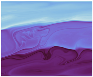
In figure 1 we show vertical cross-sections of density distributions for two cases. With the non-dimensionalisation described in the previous section, the density varies from one at the lower boundary $z=0$ to zero at the upper boundary $z=1$. The initially locally unstable stratification generates convective flows, which in turn develop into spanwise vortices due to the vertical shearing, somewhat reminiscent of Kelvin–Helmholtz (KH) billows. These vortices in turn evolve in a way that leads to layering in the scalar field. For the 3D case 1, with the smallest considered $Ra_\theta$, these KH vortices occupy the whole channel. For the cases with higher $Ra_\theta$, the vertical extent of the vortices decreases. Multiple layers emerge, separated by relatively sharp interfaces, as shown, for example, in figure 1($d$). The sharp interfaces refer to the relatively thin regions of substantially enhanced scalar gradients. Clearly, two sharp interfaces exist for the 2D case 5 with $Ra_\theta =10^7$. They oscillate strongly in space and interact with the convection flow in the relatively well-mixed layers, but the interfaces remain robust. This behaviour can be clearly seen in the supplementary movies (available at https://doi.org/10.1017/jfm.2021.1091), showing for all cases the time evolution of the two scalars independently and in combination as the density. There are some structures that are reminiscent of the classical finite-amplitude ‘cusped waves’, the finite-amplitude manifestation of the HWI (see, for example, Salehipour et al. Reference Salehipour, Caulfield and Peltier2016). Similar phenomena are also noted by Brown & Radko (Reference Brown and Radko2021) in sheared diffusive DDC. However, it is challenging to identify these structures categorically as HWI, as any impinging vortical structures are likely to induce such scouring motions in the vicinity of a sharp interface.

Figure 1. Density fields at different stages of (a,c) case 1 with $Ra_\theta =10^5$ and (b,d) case 5 with $Ra_\theta =10^7$. Panels ($a$) and ($b$) show the flow fields at the early stage when the initial perturbations grow into layers of vortices. Panels ($c$) and ($d$) show those at the final stage with distinct layers separated by sharp interfaces with high density gradient. The 3D data are from the $y$–$z$ plane at the $x$ midpoint of the computational domain. In both cases, the emergence of the layers and subsequently their coarsening with time is clearly seen. All panels share the same colour map as shown at the left.

Moreover, figure 1 illustrates why very fine grids are needed for the current study. The interfaces with relatively high density gradient have very small vertical extent, while the convective plumes emerging from these interfaces are also very narrow, requiring a very high resolution.

To verify that 2D simulations exhibit similar dynamics to 3D simulations, we compare the 2D case 3 to the 3D case 2. Both cases have the same control parameters. Flow fields are compared in figure 2 at two stages: the relatively early shear-induced KH vortices stage at $t=100$; and the later layering stage at $t=2500$. The flow morphology is largely similar in two and three dimensions. For both simulations, a single sharp interface remains during the late layering stage, though the oscillation of the interfaces is stronger in the 2D case than in the 3D case. This is perhaps unsurprising since in the 2D case the flow has fewer degrees of freedom to develop and evolve, resulting in violent fluctuations about the equilibrium state.

Figure 2. Density fields from the 3D simulation of case 2 (a,c) and the 2D simulation of case 3 (b,d). The two cases have the same $Ra=10^6$. Panels (a) and (b) are for time $t=100$ and panels (c) and (d) for $t=2500$. The 3D data are from the $y$–$z$ plane at the $x$ midpoint of the computational domain. All panels share the same colour map as shown at the left.

In figure 3 we plot the time evolution of the horizontally averaged mean profiles of non-dimensional temperature $\langle \theta \rangle _h$, salinity 〈s〉_h and density. Here $\langle \cdot \rangle _h$ stands for the spatial average over horizontal planes. With the non-dimensionalisation described in the previous section, temperature and salinity also both vary from one at the lower boundary $z=0$ to zero at the upper boundary $z=1$. Clearly, a robust staircase appears and survives for all five cases, but the time evolution varies significantly. Furthermore, the strong oscillation of interfaces is apparent. For case 1 with the smallest ${\textit {Ra}}$, once the instability triggers the flow, a single layer quickly develops and extends over the entire interior of the flow. For cases with higher ${\textit {Ra}}$, the layering process is more complex. For case 2, starting from $t\approx 1000$, two relatively weak interfaces appear in the centre of the channel. The two interfaces rapidly merge into a single one at around $t\approx 2100$.

Figure 3. Time evolution of horizontally averaged scalar profiles. Panels (a)–(e) are for cases 1–3, 5 and 6, with parameters given in table 1. Columns from left to right show mean profiles of non-dimensional temperature, salinity and density, respectively. Different cases share the same colour map for each scalar field.

By comparing rows ($b$) and ($c$) in figure 3, it is again apparent that 2D and 3D simulations have essentially similar layering processes. As $Ra_\theta$ increases, more layers appear in the interior, as seen from figure 3($d,e$) for $Ra_\theta =10^7$ and $10^8$. For case 6, the simulation with the highest $Ra_\theta$ in our study, more layer merging occurs at later times. We continued the simulation until $t=12\,000$ and only four interfaces remained. It is important to note that the depth of the final layers is much larger than the characteristic depth of the initial perturbation $1/k$. Thus, we believe it is unlikely that the depth of the final layers is set by the vertical wavenumber of the initial perturbation. Rather, the depth of the final layers is due to the competition between different layers, as well as the confinement of the two boundaries.

4. Vertical transport in layering state

Having considered qualitative aspects of the formation and survival of layered states, we now focus on the dynamics of case 5. This case clearly had a robust ‘staircase’ at later times, and we are interested in the consequences of this staircase for the global transport and flow velocities. Throughout the simulation we record the appropriately scaled global heat and salt transfer rates as well as the flow velocity. These are quantified by appropriately defined Nusselt numbers and Reynolds numbers,

(4.1a–c)\begin{equation} {\textit{Nu}}_s = \frac{\langle u_z s \rangle_a}{\kappa_s \varDelta_s H^{{-}1}},\quad {\textit{Nu}}_\theta = \frac{\langle u_z \theta \rangle_a}{\kappa_\theta \varDelta_\theta H^{{-}1}},\quad Re_i = \frac{u^{rms}_{i} H}{\nu}. \end{equation}

Hereafter $\langle \cdot \rangle _a$ denotes the volume average over the whole flow domain. These volume averages in general depend on time. The three $u^{rms}_i$ are the root-mean-square values of the different components of the total velocity, including in particular the mean imposed shear. The density $\rho '$ and its associated volume-averaged convective flux $\langle u_z\rho ' \rangle _a$ are also calculated. Figure 4 plots the time history of the global fluxes and Reynolds numbers for case 5 with $Ra_\theta =10^7$.

Figure 4. Time history of (a) the scaled global salt transfer rate ${\textit {Nu}}_s$, (b) the scaled global heat transfer rate ${\textit {Nu}}_\theta$, (c) the convective density flux $-\langle u_z\rho ' \rangle _a$, and (d,e) the Reynolds numbers $Re_y$ and $Re_z$, respectively, for case  5.

In figure 4, two qualitatively different stages can be identified after the rapid initial spin-up of the flow, which ends around $t=100$. The first stage occurs for $t \lesssim 2000$. During this initial stage, the flow interior is dominated by KH-like shear-driven vortices. This stage ends when the flow relatively quickly reorganises into the layering state for $2000 \lesssim t \lesssim 2500$. During this transition period the KH-like vortices lose their spatially organised pattern and quickly break into turbulent convection layers. Such a process can also be observed in supplementary movies 5 and 6. Subsequently, global fluxes, as quantified by the Nusselt numbers, are both typically much larger in magnitude, and also fluctuate with a much larger magnitude. These fluctuations in the global quantities are caused by the strong oscillations of the interfaces, which can also be observed in the time history of the scalar mean profiles, as shown in figure 3. The strong oscillation of the interfaces is induced by the violent convection motions in the adjacent layers. During the final stage, the equilibrium layering state can survive these strong oscillations for a very long time period. Also, for our choice of control parameters, the streamwise Reynolds number $Re_y$ is always significantly larger than the vertical Reynolds number $Re_z$, due to the contribution from the mean shear.

To reveal the effects of different structures on the transport properties, we calculated the time history of horizontally averaged vertical profiles of scalar gradient $\langle \partial _z \zeta \rangle _h$, scalar convective flux $\langle u_z \zeta \rangle _h$ and turbulent diffusivity $\kappa ^T_\zeta = \langle u_z\zeta \rangle _h / \langle \partial _z\zeta \rangle _h$, for the three scalars of interest with $\zeta =\theta$, $s$ and $\rho '$. Figure 5 displays these time histories, once again for case 5. The staircase structure of thin interfaces and relatively deep layers is clearly apparent in figure 5($a$–$c$). The dark blue stripes mark the interfaces which have relatively high gradients of temperature, salinity and density. The negative vertical gradient arises since both temperature and salinity decrease as the height increases, with salt stabilising and heat destabilising the flow statically. The relatively vertically extended white regions between interfaces with relatively weak gradients are the well-mixed layers with almost homogeneous mean temperature and salinity. Figure 5($c$) indicates that, inside the layers, the density often exhibits a slightly positive net mean gradient, and it is this convectively unstable stratification that drives the large roll convection inside these layers, even though, overall, the density gradient is stable across the flow.

Figure 5. Time evolutions of the horizontally averaged profiles for case 5. Rows from top to bottom show mean profiles of scalar gradients $\langle \partial _z\zeta \rangle _h$, scalar convective fluxes $\langle u_z\zeta \rangle _h$ and turbulent diffusivity $\kappa ^T_\zeta = \langle u_z\zeta \rangle _h / \langle \partial _z\zeta \rangle _h$. Columns from left to right are for $\zeta =\theta$, $s$ and $\rho '$, respectively. Black arrows mark the time-averaged heights of identifiable interfaces.

As expected, the convective fluxes $\langle u_z\zeta \rangle _h$ for the three different scalars show very different behaviours in the interface and layer regions. The interface regions consist of strong oscillations between extreme positive and negative convective fluxes of heat, salinity and density. This is essentially a geometric effect, caused by the vertical spatial oscillations of the interfaces, in turn associated with the coupled effects of impinging vortices and ejecting plumes, as can be seen in the supplementary movie. Nevertheless, the interfaces with strong scalar gradients survive these spatial oscillations in our simulations. In the interior of layers, oscillations are also observed in the convective fluxes, but overall $\langle u_z\theta \rangle _h$ and $\langle u_z s \rangle _h$ are positive, implying that both heat and salinity are transferred upwards.

Meanwhile, the convective flux of $\rho '$ is negative inside layers, indicating that the net density flux is actually downwards in the layers as expected. This is consistent with the regular occurrence of static instability in the layers, and also with the density flux being dominated by the thermal convective component. This confirms that the shear has not qualitatively affected the distinguishing characteristic of diffusive DDC of downward density flux. In figure 5($g$–$i$) we plot the mean profiles of turbulent diffusivities $\kappa ^T_\zeta = \langle u_z\zeta \rangle _h / \langle \partial _z\zeta \rangle _h$. The most intense turbulent diffusivity actually occurs inside the layers, where the magnitude of $\kappa ^T_{\rho '}$ can be larger than $0.01$. It can also be noted that, at the interface regions, the turbulent diffusivities computed from horizontally averaged profiles have comparable values for temperature and salinity. However, within the layers, the magnitude of $\kappa ^T_\theta$ is much larger than $\kappa ^T_s$. This implies that, within the layers, the flow is not in a fully developed turbulent state in our simulations, since for fully developed turbulent flow the convective fluxes should be similar for the two components.

In figure 6, we plot time averages over the time period $3000< t<6000$ of the horizontally averaged mean profiles shown in figure 5, as well as the flux ratio $\gamma ^*$, defined as the ratio of the total salt flux to the total heat flux,

(4.2)\begin{equation} \gamma^*(z) = \frac{\beta_s (\langle w_{dim} s_{dim} \rangle _h + \kappa_s \partial _z \langle s \rangle_h )} {\beta_\theta (\langle w_{dim} \theta_{dim} \rangle _h + \kappa_\theta \partial _z \langle \theta_{dim} \rangle_h )}, \end{equation}

where the subscripts ${dim}$ make explicit that the definition contains dimensional quantities and the total flux contains both convective and diffusive parts. Although in principle $\gamma ^*(z)$ can vary with $z$, at a statistically stationary state both denominator and numerator should be constant with height.

Figure 6. Time-averaged profiles for (a–c) the three scalar fields, (d–f) their convective fluxes and (g) the total flux ratio $\gamma ^*$, as defined in (4.2). Time averaging is calculated from the data presented in figure 5 over the time interval $3000 \leq t \leq 6000$.

Owing to the vigorous and relatively high-amplitude vertical oscillations of the interfaces, the time-averaged scalar profiles do not exhibit sharp interfaces but rather regions with relatively high gradient, near $z \simeq 0.3$ and $z \simeq 0.65$, as shown in figure 6($a$–$c$). Interestingly, although such spatial oscillations generate large, and yet crucially temporally varying, local vertical fluxes, as shown in figure 5, after time averaging the interface regions exhibit smaller net convective heat flux. Upon time averaging, the positive and negative fluxes with large magnitude visible in figure 5 associated with the significant convective deformations of the interfaces exhibit significant cancellation. Therefore, the net convective transport across the interfaces is substantially reduced. Conversely, the transport through the relatively well-mixed layers does not exhibit such variability, and in particular is typically single-signed, and so the net convective transport through the layers is significantly larger. Of course, this variability is counterbalanced by the stronger diffusive flux through the high-gradient interfaces. It is also important to appreciate that, instantaneously, the transport across an interface can be very much larger in magnitude and opposite in sign to the net transport over a sufficiently long time interval, strongly suggestive of the physical mechanisms that lead to staircase structures having reduced net vertical transport.

Furthermore, the convective density flux is dominated by the heat flux. The net salinity flux is both significantly smaller in magnitude and also much closer to uniform across the entire flow, with no noticeable remnant remaining of the staircase structure in the time-averaged convective flux. Since the salinity is higher at the bottom boundary and lower at the top, it is reasonable to expect the convective part of the salinity flux to be positive, i.e. in the opposite direction to the total salinity gradient across the whole fluid layer. Indeed, this is observed, albeit with very small magnitude. Nevertheless, it is important to appreciate that the overall net convective density flux is negative, and hence downwards, even though the flow is statically stable, and so the flux here might be appropriately described as counter-gradient, in the sense that the net background density gradient is also negative, as is of course to be expected for DDC in the diffusive regime considered here. Interestingly, the middle layer is, upon this long-time averaging, statically stable, while the upper and lower layers are statically unstable. This qualitative difference is not reflected in the density flux within the layers, which is dominated by the vertical flux of heat, and largely takes similar values in each of the three layers. Clearly, from the time evolution data shown in figure 5, each of the layers is frequently statically unstable, and thus associated with vigorous convective overturning, and so it is not appropriate to draw any inferences from the long-time-averaged static stability of the middle layer.

Finally, the total flux ratio $\gamma ^*(z)$ shown in figure 6($g$) hardly varies with $z$ over the flow domain, giving further confidence to the assertion that the flow is essentially in a statistically steady state. More interestingly, $\gamma ^* \simeq 0.1 =\sqrt {\tau }$, remembering the definition of the diffusivity ratio (2.5). This is entirely consistent with the physical arguments presented by Linden & Shirtcliffe (Reference Linden and Shirtcliffe1978) considering idealised two-layer systems (see also Worster Reference Worster2004). The key insight presented by Linden & Shirtcliffe (Reference Linden and Shirtcliffe1978) is that, within the interfacial ‘boundary layers’, salt diffuses in the thermally convective elements, which then break away and are mixed into the ‘bulk’ layers. This fundamental picture does not appear to be disrupted in any significant way by the presence of mean shear, augmenting the vortical scouring of the interfaces. Indeed, our results appear to give strong support to the variational arguments of Stern (Reference Stern1982) that $\gamma ^*$ should be bounded below by $\sqrt {\tau }$. Furthermore, our choice of density ratio $\varLambda =2$ is both in the range $\varLambda < \tau ^{-1/2}$ where the original model of Linden & Shirtcliffe (Reference Linden and Shirtcliffe1978) admits steady-state solutions, and also at the start of the constant regime with uniform flux ratio $\gamma ^* \simeq 0.13$ observed experimentally by Turner (Reference Turner1965). As discussed in detail by Worster (Reference Worster2004), there are several complicating issues in experimental realisations of diffusive DDC, whereas numerically it is straightforward to maintain constant boundary conditions for the salinity and temperature.

Although the flux ratio does not appear to show any effect of the shear-driven forcing, i.e. not varying significantly in the vertical direction, it is still natural to be interested in the spatio-temporal properties of the scalar transport, particularly in such a controlled sheared and overall statically stable flow. In single-scalar stratified shear flows, it is commonplace to consider the ‘efficiency’ of the shear-driven transport, which is traditionally quantified by an appropriately defined turbulent flux coefficient, $\varGamma$. As introduced by Osborn (Reference Osborn1980), $\varGamma$ is the ratio of the vertical density flux to the turbulent kinetic energy dissipation rate. In a statistically stationary flow where transport terms into and out of the domain can be ignored, and the turbulent kinetic energy is essentially constant, this ratio may be expected to quantify the relative strength of the density flux and viscous dissipation. For statically stable single-component flows, the density flux may be related to irreversible changes in the potential energy. As here we are particularly interested in the dynamics of staircases, which exhibit spatial variation in the vertical direction, and specifically the transport properties of layers and interfaces, it is natural to define a flux coefficient as a function of $z$ and $t$ as

(4.3)\begin{equation} \varGamma(z,t)= \frac{g\langle u_z\rho' \rangle_h}{\langle\varepsilon\rangle_h}, \end{equation}

where $\varepsilon$ is the local, pointwise dissipation rate of the total kinetic energy.

It is important to appreciate that, defined in this way, $\varGamma (z,t)$ is sign-indefinite due to sign-indefinite horizontally averaged density flux in its numerator. Thus, $\varGamma$ will only be positive when, on average, dense parcels of fluid are being lifted up, as might be expected in statically stable turbulent shear flows with a single component in a statistically steady state, but of course does not happen typically in diffusive DDC, even when sheared, as we have observed above. Indeed, in single-component statically stable stratified flows, there has been much research devoted to attempts to go beyond the classical empirical observation of Osborn (Reference Osborn1980) that $\varGamma \lesssim 0.2$ to identify generic parametrisations of $\varGamma$ in terms of other parameters describing properties of the fluid, larger-scale flow properties and/or turbulence (see, for example, Caulfield (Reference Caulfield2021) for a review). Two particular parameters of interest are appropriately defined gradient Richardson numbers $Ri_g(z,t)$ and buoyancy Reynolds number $Re_b(z,t)$:

(4.4a–c)\begin{equation} {\textit{Ri}}_g (z,t)= \frac{N^2}{S^2},\quad Re_b(z,t) = \frac{\langle\varepsilon\rangle_h}{\nu N^2},\quad N^2 =\partial_z\langle g\rho' \rangle_h. \end{equation}

Here, for consistency with the chosen definition of $\varGamma$, the buoyancy frequency $N^2$ and the background shear $S=\partial _z\langle u_y \rangle _h$ are defined in terms of horizontally averaged quantities. Therefore, both ${\textit {Ri}}_g$ and $Re_b$ may in general vary with vertical location and time, and, as $N^2$ is only positive when the horizontally averaged flow is statically stable, it is important to remember that both ${\textit {Ri}}_g$ and $Re_b$ can in principle be negative, quite possibly within the layers, though the interfaces should still exhibit positive values. It should also be mentioned that $Re_b$ has been used to identify different regimes of mixing, namely a molecular regime, a transition regime and a fully energetic regime (Ivey, Winters & Koseff Reference Ivey, Winters and Koseff2008).

Indeed, in figure 7 we show the time history for the profiles of the three quantities defined in (4.3) and (4.4a–c). As expected, after the initial transient to the asymptotic three-layer state, ${\textit {Ri}}_g$ and $Re_b$ display opposite behaviours in the interface and layer regions. Specifically, near interfaces, ${\textit {Ri}}_g$ is large and $Re_b$ is small, attributable to the high density gradients. Conversely, within layers, $Re_b$ with large magnitude is associated with small-in-magnitude ${\textit {Ri}}_g$, with evidence of both positive and negative values for both parameters, corresponding to the convection motions. In figure 7($c$), it is evident that the ratio $\varGamma$ fluctuates very strongly near interfaces, attaining both positive and negative values with large magnitude. This suggests that the local dissipation rate being small near interfaces is dominating the observed numerical values, with the strong fluctuation of $\varGamma$ being clearly induced by the spatial oscillation of interfaces.

Figure 7. Time evolutions for profiles of (a) ${\textit {Ri}}_g$ (b) $Re_b$, and (c) $\varGamma$, respectively, for case 5 with $Ra_\theta =10^7$. Black arrows mark the heights of interfaces.

A useful way to understand the relationship between the various quantities is to calculate the joint probability of pairs of quantities associated with specific values of $z$ and $t$. We present joint probability density functions (p.d.f.s) for these data for four pairs of quantities in figure 8. Figure 8(a) shows the joint probability of $\langle -\partial _z \rho ' \rangle _h$ and $\langle u_z\rho ' \rangle _h$. Indicating that most of the flow domain is in relatively well-mixed layers, most of the data are associated with values of the mean density gradient being close to zero, though both positive and negative small gradients occur frequently. Conversely, there is a strong signal of predominantly negative density flux, associated with the expected strong convective flux of heat through the system, and particularly in the layers. Inside the layers the fluid is well mixed with nearly homogeneous mean scalars and so large-scale convection rolls generate high convective flux. Unsurprisingly, there is asymmetry in the data associated with the existence of interfaces with high horizontally averaged negative density gradient. The associated values of convective flux are spread over a wide range, which can be interpreted as being due to the significant spatial oscillation of interfaces.

Figure 8. Joint relative probability for four pairs of flow quantities, including the vertical gradient of mean density $\langle -\partial _z \rho ' \rangle _h$, the mean convective flux of density $\langle u_z\rho ' \rangle _h$, $\varGamma =g\langle u_z\rho ' \rangle _h / \rho _0\langle \varepsilon \rangle _h$, ${\textit {Ri}}_g=N^2/S^2$ and $Re_b = \langle \varepsilon \rangle _h/\nu N^2$. Statistics are calculated from the data of figure 5 for $t>3000$ and $0.1< z/H<0.9$. The colour is shown on logarithmic scale.

In figures 8(b) and 8(c) we show the joint p.d.f.s of $\varGamma$ with ${\textit {Ri}}_g$ and $Re_b$, respectively. The ${\textit {Ri}}_g$ data in figure 8(b) are once again dominated by values with relatively small magnitude, associated with most of the flow domain being in layers. Both negative and positive values are apparent, showing that the layers oscillated close to being well mixed, while $\varGamma$ is clearly predominantly negative, since there is typically downward convective density flux. Once again, there is asymmetry in the ${\textit {Ri}}_g$ data, with a wide range of positive values associated with the interfaces, associated also with a very wide range of different $\varGamma$ values.

Large-magnitude values of $\varGamma$ are of course associated with significant density flux with relatively weak turbulence, precisely the behaviour that we would expect in the vicinity of a highly convoluted yet ‘sharp’ interface dominated by scouring dynamics. Such apparently weak turbulence leading to significant convective transport is also apparent in the $\varGamma (Re_b)$ data shown in figure 8(c). The data associated with the interfaces, with small positive $Re$ due to the combined effect of small $\varepsilon$ and large $N^2$ and a wide range of large-magnitude $\varGamma$, are clearly apparent. Conversely, the layer data exhibit a wide range of both positive and negative $Re_b$ with predominantly smaller yet negative  $\varGamma$.

Indeed, figures 8(b) and 8(c) strongly suggest that ${\textit {Ri}}_g$ and $Re_b$ are anticorrelated, as can also be seen in figure 8(d). The expected asymmetry in data is clearly visible, where large positive ${\textit {Ri}}_g$ associated with interfaces is much more common than large negative values. The large positive ${\textit {Ri}}_g$ data correspond to small positive values of $Re_b$. Conversely, layers are associated with large-in-magnitude $Re_b$ data and small-in-magnitude ${\textit {Ri}}_g$, with both signs commonly occurring. We plot the heuristic relationship ${\textit {Ri}}_g \propto Re_b^{-1}$ with a red dashed line, which appears to be a reasonable approximation. This suggests that the dominant relationship is associated with the density distribution via the respective dependence on $N^2$ in the parameter definitions, and variations in the mean shear and dissipation rate only play a role at higher order.

As a final demonstration of the properties of the convective fluxes of different flow regions, in figure 9 we plot the time average over the interval $3000 < t < 6000$ of the negative of the density flux $\langle -u_z\rho ' \rangle _h$ conditioned on $\langle -\partial _z \rho ' \rangle _h$. A single peak appears, with $\langle -\partial _z \rho ' \rangle _h$ slightly smaller than zero, corresponding to regions of the flow with weak statically unstable density gradients. Such regions correspond naturally to the relatively well-mixed ‘layers’. As $\langle -\partial _z \rho ' \rangle _h$ increases through positive values, the magnitude of the conditioned average broadly decreases. Higher values of the density gradient are naturally found in the interface regions, where the convective flux becomes relatively weak. As is apparent in figure 5, the particular location of such interfaces generically oscillates very strongly and it is therefore entirely reasonable that the convective flux exhibits significant fluctuations. Nevertheless, the conditioned average shown in figure 9 suggests that the net overall convective density flux in the interface regions is still negative, although the interfaces drive a downward density convective flux that is much weaker than that which is driven through the layers. This is yet more evidence that the strong shear present in such flows does not modify the overall downward density flux characteristic of diffusive DDC flows, due to the dominance of the upward convective heat flux.

Figure 9. Time average (over the interval $3000 < t < 6000$) of the mean convection flux $\langle u_z\rho ' \rangle _h$ conditioned on the mean density gradient $\langle -\partial _z \rho ' \rangle _h$.

5. Development of local density inversion and multiple states of layering

Another interesting property of the sheared diffusive DDC flows considered here is that the final configuration of layering actually depends on the particular structure of the initial perturbation, in a non-trivial fashion. The coexistence of various layered states has been hypothesised by Stern & Turner (Reference Stern and Turner1969) as metastable equilibria of the system. To demonstrate this, we consider the properties of case 7. As discussed in § 2, case 7 has the same flow control parameters as case 5 but a different, and more localised, initial condition, given by (2.8a,b) rather than (2.6a,b). Analogously to figure 3, we show the time evolution of the scalar profiles for case 7 in figure 10. Also in figure 11 we show the contours of density at four different times.

Figure 10. Time evolutions of the horizontally averaged scalar profiles for case 7, starting from a single localised density inversion, with control parameters the same as case 5, as listed in table 1: (a) temperature, (b)  salinity and (c)  density.

Figure 11. Snapshots of density at four different time steps for case 7: (a) $t = 10\,000$, (b) $t = 12\,000$, (c) $t = 16\,500$ and (d) $t = 20\,000$.

Initially, the single density inversion expands vertically over a sustained time period of more than 10 000 non-dimensional time units. As is typical, KH-like vortices grow within this expanding layer and then in turn break down into a well-mixed convection layer. Around $t=12\,000$, two new, essentially well-mixed, layers emerge above and below the primary layer. However, these two relatively new layers are continually eroded, as is apparent in figure 11($c$). Indeed, they do not survive and the main layer in the middle eventually occupies the whole channel, leading to a statistically steady state with a single convection layer, in qualitative contrast to the flow field shown in figure 1 for the corresponding case 5. Therefore, for the same control parameters, different statistically steady states can be achieved starting from different initial density conditions. Without the presence of other layers, a single layer can grow continuously until the confinement of the boundaries sets in. Crucially, the various fluxes are also different for different states. The existence of multiple turbulent states with different transport properties has also been observed in other turbulent systems such as in Taylor–Couette flow (Huisman et al. Reference Huisman, van der Veen, Sun and Lohse2014) and fingering DDC staircases (Yang et al. Reference Yang, Chen, Verzicco and Lohse2020).

In figure 12 we plot the time history of the two Nusselt numbers and the vertical flux of the density. During the multilayer stage between $t=16\,000$ and $18\,000$, the fluxes fluctuate significantly. When the flow enters the single-layer final stage after $t>18\,000$, both the heat and density fluxes increase and fluctuate more strongly. The fluctuation of salinity flux, however, reduces significantly.

Figure 12. Time history of (a) the scaled global salt transfer rate ${\textit {Nu}}_s$, (b) the scaled global heat transfer rates ${\textit {Nu}}_\theta$ and (c) the convective density flux $-\langle u_z\rho ' \rangle _a$ for case 7, as listed in table 1.

For cases 5 and 7 with $Ra=10^7$ and different initial perturbations, we measure the time-averaged fluxes at the final statistically steady stage for both the three-layer state of case 5 and the single-layer state of case 7. We average between $t=4000$ and $6000$ in figure 4 for the three-layer state, and between $t=19\,000$ and $20\,000$ in figure 12 for the single-layer state. The two Nusselt numbers are ${\textit {Nu}}_\theta =3.73$ and ${\textit {Nu}}_s=20.9$ for the three-layer state, and ${\textit {Nu}}_\theta =9.03$ and ${\textit {Nu}}_s=37.1$ for the single-layer state, respectively. Therefore, under the same global control parameters, more layers and interfaces really significantly reduce the heat and salinity transport in the vertical direction, showing how important layering can be for ‘throttling’ vertical fluxes, and so how crucial it is to understand whether a particular staircase arrangement is robust and long-lived when subject to velocity shear, and hence further vigorous forcing.