


1. Introduction
The flow area of nozzles and diffusers changes as a function of their distance along the component, and the flow field should therefore be at least two-dimensional for symmetrical components. However, an assumption is often made that the flow properties only vary along the axes of nozzles and diffusers adopting a one-dimensional description: this is equivalent to assuming uniform flow properties over any given cross-section. Such an approach is often defined as quasi-one-dimensional (Anderson Reference Anderson1995) and it represents a simplified model of the phenomena.
Many fluid dynamics processes and research themes, such as the interaction between shocks and boundary layers, free shock separation in over-expanded jets (Martelli et al. Reference Martelli, Saccoccio, Ciottoli, Tinney, Baars and Bernardini2020), entrance effects due to the developing internal flow (Kohl et al. Reference Kohl, Abdel-Khalik, Jeter and Sadowski2005), turbulence and vorticity (Mahapatra et al. Reference Mahapatra, Nelaturi, Tennyson and Ghosh2019), entropy noise (Emmanuelli et al. Reference Emmanuelli, Zheng, Huet, Giauque, Le Garrec and Ducruix2020), reactive flows and the prediction of resonance in nozzle flows (Zaman et al. Reference Zaman, Dahl, Bencic and Loh2002), require a multi-dimensional modelling of nozzles, diffusers and ducts. However, (quasi-) one-dimensional models continue to attract attention for a variety of technological applications (Maicke & Bondarev Reference Maicke and Bondarev2017). Their surprising simplicity is responsible for their wide acceptance in both academic and industrial circles. Most of the conceptual research on advanced numerical methods for the control of oscillations in the simulation of weak solutions is based on the analysis of the results of one-dimensional equations (Toro Reference Toro2009).
The one-dimensional models are popular in the engineering communities that deal with propulsion and power generation equipment (Maicke & Majdalani Reference Maicke and Majdalani2012): applications abound and include wind tunnels (Rodriguez Lastra et al. Reference Rodriguez Lastra, Fernandez Oro, Vega Galdo, Marigorta Blanco and Morros Santolaria2013), scramjets (Yu et al. Reference Yu, Chen, Huang, Lv and Xu2020), rockets (Sutton Reference Sutton1992), ramjets, afterburners and a variety of gas turbine components through which gases are expanded (Maicke & Majdalani Reference Maicke and Majdalani2012; Cavazzuti & Corticelli Reference Cavazzuti and Corticelli2017). With the development of micro-machine technology, numerous research investigations on viscous gaseous flows in micro-channels have also been carried out with one-dimensional models in the microelectronic and bioengineering fields (Atmaca, Erek & Ekren Reference Atmaca, Erek and Ekren2020; Martelli et al. Reference Martelli, Saccoccio, Ciottoli, Tinney, Baars and Bernardini2020).
Only numerical solutions can be obtained for one-dimensional unsteady compressible viscous diabatic flows in nozzles, diffusers and ducts, once suitable boundary conditions have been assigned. When the kinetic energy of the flow is significant and cannot be disregarded, as occurs in the gas dynamics field, the steady-state one-dimensional equations can admit an exact solution for a few known cases.
If the heat transfer is negligible and the viscous flow occurs along a constant cross-section pipe, the exact solution can be expressed by means of Fanno's analytical model (1904), which was originally used for subsonic flows and then extended to supersonic flows (Kirkland Reference Kirkland2019). On the other hand, if the heat transfer is significant, friction is negligible and the flow occurs along a constant cross-section pipe, the Rayleigh model (1910) can be used to determine the exact solution (Anderson Reference Anderson2003). Finally, when both the friction and heat transfer can be disregarded and the steady-state adiabatic inviscid flow evolution is caused by the variable cross-section of the pipe along its axis, the exact solution is calculated by means of the popular nozzle flow model (Moran et al. Reference Moran, Shapiro, Boettner and Bailey2010) that was developed by different scientists between the mid-1890s and mid-1900s.
All the above-mentioned exact models only take into account a single flow variation effect (friction, heat transfer or gradual change in the flow area) and for this reason they are also referred to as simple flows (Shapiro Reference Shapiro1953). Shapiro determined an exact solution, assuming an isothermal flow, for the simulation of both friction and heat transfer effects along a constant cross-section pipe. The general case of viscous diabatic flow, without the assumption of barotropic evolution (Prud'homme Reference Prud'homme2010), has only recently been solved analytically (Ferrari Reference Ferrari2020). Instead, there are no available solutions for the steady-state problem, in closed form, for a compressible viscous flow through a variable cross-section pipe: the generally adopted methodology involves calibrating the isentropic model using empirical factors for a given viscous gas, or applying other empirical models (Senftle et al. Reference Senftle, Michael, Thorpe, James and Grant2003). In fact, exact solutions can only be determined for a variable area Fanno flow if an additional function, which relates the change in pressure to the change in area, is hypothesised for the pipe (Loh Reference Loh1970), but such a function is generally unknown a priori.
In this paper, we analytically solve compressible viscous flows that include both friction and variable cross-section effects in the presence of significant kinetic energy and possible shocks for conical nozzles and diffusers. An analysis of the design and off-design conditions is also provided for conical pipes, and choking conditions are discussed to guide the physical interpretation of the obtained analytical distributions.
The provided solutions, which have been validated by means of a comparison with the outcomes of numerical models, extend the collection of exact solutions of gas dynamics and may be useful for the evaluation of numerical schemes and for technological applications (Hasselmann, der Wiesche & Kenig Reference Hasselmann, der Wiesche and Kenig2019). In the latter case, the analytical laws offered by the exact solutions provide an efficient means of evaluating the cause-and-effect relationships between the geometrical and physical parameters of the problem and the unknown variables of the ordinary differential equations (ODEs), whereas two-dimensional (2-D) numerical simulations are more cumbersome and only allow parametric analyses to be performed. However, the results of these parametric analyses cannot be synthetized with a mathematical expression.
2. Differential equations of the gas dynamics problem
Generalised Euler partial differential equations (PDEs) for a quasi-one-dimensional unsteady viscous diabatic compressible flow through nozzles and diffusers are given by (gravity is neglected) (Bermudez, Lopez & Vasquez-Cendon Reference Bermudez, Lopez and Vasquez-Cendon2017)
 \begin{equation}\left. {\begin{array}{c@{}} {\dfrac{{\partial (\rho A)}}{{\partial t}} + \dfrac{{\partial (\rho Au)}}{{\partial x}} = 0}\\ {\dfrac{{\partial (\rho uA)}}{{\partial t}} + \dfrac{{\partial (pA + \rho {\kern 1pt} {u^2}A)}}{{\partial x}} ={-} \mathrm{\pi }D{\tau_w} + p\dfrac{{\partial A}}{{\partial x}}}\\ {\dfrac{{\partial (\rho {e^0}A)}}{{\partial t}} + \dfrac{{\partial (A\rho u{h^0})}}{{\partial x}} = \mathrm{\pi }D{{\dot{q}}_f}} \end{array}} \right\},\end{equation}
where t is the time, x is the space coordinate, ρ, u and p are the cross-sectionally averaged 1-D density, velocity and pressure, respectively, A = A(x) is the variable pipe cross-section, D = D(x) is the variable diameter, e 0 is the stagnation internal energy (e 0 = e + u 2/2, where e is the internal energy), h 0 is the stagnation enthalpy (h 0 = h + u 2/2, where h is the enthalpy), τw is the wall friction shear stress and  ${\dot{q}_f}$ is the heat flux with the walls. Equation (2.1) differs from the standard set of Euler equations for an isentropic flow because the friction and heat exchange are added on the right-hand side and evaluated as volume source terms (Hirsch Reference Hirsch2007; Maeda & Colonius Reference Maeda and Colonius2017) using Darcy–Weisbach's wall friction and convective heat transfer models. Equation (2.1) is a simplified approach compared to the Navier--Stokes equations, which use a multidimensional diffusive transport mechanism to model viscous stress and conductive heat. Wall friction stress can be modelled in (2.1) with (White Reference White2015)
 \begin{equation}{\tau _w} = \frac{f}{2}\rho {u^2},\end{equation}
where the friction coefficient f can be expressed as a function of the Reynolds number Re = ρuD/μ for a laminar flow, with μ being the dynamical viscosity of the fluid, and as a function of both Re and the relative roughness ε/D for a turbulent flow, with ε being the average roughness of the wall. Either Moody's diagram or both the 16/Re formula for a laminar flow (Re < 2000) and Colebrook–White's implicit equation for a turbulent flow (4000 < Re < 108, 10−6 < ε/D < 10−2) can be used to evaluate f (Douglas et al. Reference Douglas, Gasiorek, Swaffield and Jack2005; White Reference White2015). An updated review of the most refined explicit formulas used in the literature to calculate f, as a function of Re and ε/D, is reported in Cheng (Reference Cheng2008). More accurate correlations, in which f generally depends on Re, ε/D and the Mach number are reported in Schwartz (Reference Schwartz1987), Asako et al. (Reference Asako, Pi, Turner and Faghri2003), Hong et al. (Reference Hong, Nakamura, Asako and Ueno2016).
According to a convective heat transfer model, the heat flux  ${\dot{q}_f}$ in (2.1) is a function of the cross-sectionally averaged one-dimensional temperature (T) of the fluid, through a convective heat transfer coefficient that depends on Re and the Prandtl number (Bejan Reference Bejan2013). In other words, although a viscous friction and heat transfer simulation should require at least a 2-D model, to take into account the axial and radial variations of the velocity and temperature, the simplified model presented here uses a 1-D approach and then compensates for this shortcoming by applying empirical factors (f and a convective heat transfer coefficient) that need complex correlations.
Equation (2.1) is completed with the following state equations:
 \begin{equation}\left. {\begin{array}{c@{}} {p = \dfrac{{\gamma - 1}}{\gamma }\rho h,\quad h = {c_p}T}\\ {h = e + \dfrac{p}{\rho },\quad e = {c_v}T} \end{array}} \right\},\end{equation}
where γ = cp/cv is the ratio of the constant pressure specific heat (cp) to the constant volume specific heat (cv) and is here considered constant, as for a standard ideal gas.
When considering steady-state flows, the partial derivatives, with respect to time, vanish in (2.1), which reduces to a system of nonlinear ODEs with respect to x (Emmons Reference Emmons1958)
 \begin{equation}\left. {\begin{array}{c@{}} {\dfrac{{\textrm{d}\dot{m}}}{{\textrm{d}x}} = 0}\\ {A\dfrac{{\textrm{d}p}}{{\textrm{d}x}} + \dot{m}\dfrac{{\textrm{d}u}}{{\textrm{d}x}} ={-} \mathrm{\pi }D{\tau_w}}\\ {\dot{m}\dfrac{{\textrm{d}{h^0}}}{{\textrm{d}x}} = \mathrm{\pi }D{{\dot{q}}_f}} \end{array}} \right\},\end{equation}
where  $\dot{m} = \rho Au$ is the constant mass flow rate through the pipe. These equations are applied to evaluate real flow evolutions in ducts, nozzles and diffusers with regular and symmetrical cross-section shapes and negligible curvature of the axis. The most accurate results for the simulation of real viscous diabatic (or adiabatic) compressible flows are obtained when
  $1/A|\textrm{d}A/\textrm{d}x|\mathrm{\Delta }x \ll 1$, where Δx is a characteristic distance, measured along the axis and related to the diameter size (Kamm & Shapiro Reference Kamm and Shapiro1979). When the radius of curvature is not large, compared with D or when
  $|\textrm{d}A/\textrm{d}x{|_{av}}\mathrm{\Delta }x \approx A$, a 2-D model is recommended for compressible flows.
3. Exact solution for compressible viscous flows in conical nozzles
Let us consider a steady-state compressible viscous adiabatic flow along a variable circular cross-section pipe with negligible curvature of the axis. The total energy conservation law in (2.4) reduces to  $({\dot{q}_f} = 0)$
 \begin{equation}{c_p}T + {\textstyle{1 \over 2}}{u^2} = {h^0} = cost.\end{equation}
The momentum balance law in (2.4) can be rewritten as follows (the momentum balance is multiplied by u and the expression of τw in (2.2) is used):
 \begin{equation}Au\frac{{\textrm{d}p}}{{\textrm{d}x}} + \dot{m}\frac{\textrm{d}}{{\textrm{d}x}}\left( {\frac{{{u^2}}}{2}} \right) + \frac{{4f}}{D}\dot{m}\left( {\frac{{{u^2}}}{2}} \right) = 0,\end{equation}
where f is here considered uniform (it can be made equal to a space-averaged value over the pipe), in line with the original Fanno flow and with several approximated solutions of compressible flows with wall friction (Parker Reference Parker1989; Shiraishi et al. Reference Shiraishi, Murayama, Kawakami and Nakano2011; Cavazzuti, Corticelli & Karayiannis Reference Cavazzuti, Corticelli and Karayiannis2019).
The pressure can be expressed with the following formula, which was obtained using the state equations of ideal gases, i.e. (2.3), in conjunction with (3.1) and the flow-rate equation  $\rho uA = \dot{m} = cost$:
 \begin{equation}p = p(u,A) = \frac{{\gamma - 1}}{\gamma }\frac{{\dot{m}}}{{Au}}h = \frac{{\gamma - 1}}{\gamma }\frac{{\dot{m}}}{{Au}}\left( {{h^0} - \frac{1}{2}{u^2}} \right).\end{equation}
The pressure gradient can thus be calculated by applying the chain rule. By using the relation  ${h^0} = {c_p}{T^0} = \gamma /(\gamma - 1)R{T^0}$, one achieves
 \begin{equation}\frac{{\textrm{d}p}}{{\textrm{d}x}} ={-} \frac{{\dot{m}}}{{{A^2}u}}R{T^0}\frac{{\textrm{d}A}}{{\textrm{d}x}} + \frac{{\dot{m}}}{{{A^2}}}\frac{{\gamma - 1}}{{2\gamma }}u\frac{{\textrm{d}A}}{{\textrm{d}x}} - \frac{{\dot{m}}}{{{Au^2}}}R{T^0}\frac{{\textrm{d}u}}{{\textrm{d}x}} - \frac{{\dot{m}}}{{2A}}\frac{{\gamma - 1}}{\gamma }\frac{{\textrm{d}u}}{{\textrm{d}x}}.\end{equation}
By substituting (3.4) in (3.2), taking into account the relation
 \begin{equation}\frac{1}{A}\frac{{\textrm{d}A}}{{\textrm{d}x}} = \frac{2}{D}\frac{{\textrm{d}D}}{{\textrm{d}x}},\end{equation}
and performing some algebraic manipulations, the following nonlinear ODE is obtained with a single unknown function, that is, the kinetic energy per unit of mass ( $y: = {u^2}/2$ for conciseness of notation):
 \begin{equation}\frac{{\gamma + 1}}{\gamma }y\frac{{\textrm{d}y}}{{\textrm{d}x}} - R{T^0}\frac{{\textrm{d}y}}{{\textrm{d}x}} = \frac{{4R{T^0}}}{D}\frac{{\textrm{d}D}}{{\textrm{d}x}}y - \left[ {\frac{{4(\gamma - 1)}}{{\gamma D}}\frac{{\textrm{d}D}}{{\textrm{d}x}} + \frac{{8f}}{D}} \right]{y^2}.\end{equation}
Equation (3.6) can be identified with the  ${g_1}y\,\textrm{d}y/\textrm{d}x + {g_0}\,\textrm{d}y/\textrm{d}x = {j_0} + {j_1}y + {j_2}{y^2}$ ODE model, which is the standard form of an Abel equation of the second kind. In the case of (3.6),
  ${g_0} = -R{T^0}$ and
  ${g_1} = (\gamma + 1)/\gamma $ are constant coefficients, that is, they are independent of x, whereas coefficients
  ${j_1} = [4R{T^0}/D \cdot \textrm{d}D/\textrm{d}x]$ and
  ${j_2} ={-} [4(\gamma - 1)/(\gamma D) \cdot \textrm{d}D/\textrm{d}x + 8f/D]$ are variable with x (the free term j 0 is null).
The variable is changed according to the following transformation (Bogouffa Reference Bogouffa2014):
 \begin{align}\frac{1}{z}: = {g_1}y + {g_0} = \frac{{\gamma + 1}}{\gamma }y - R{T^0} \Rightarrow y = \frac{\gamma }{{\gamma + 1}}\frac{{1 + R{T^0}z}}{z},\quad \frac{{\textrm{d}y}}{{\textrm{d}x}} ={-} \gamma \frac{{\textrm{d}z/\textrm{d}x}}{{(\gamma + 1){z^2}}}.\end{align}
Equation (3.6) can be reduced, after some analytical steps, to the following Abel equation of the first kind in homogeneous form, that is, without the free term
 \begin{equation}\frac{{\textrm{d}z}}{{\textrm{d}x}} = {r_0}(x) + {r_1}(x)z + {r_2}(x){z^2} + {r_3}(x){z^3},\end{equation}
where
 \begin{align}\left. {\begin{array}{c@{}} {{r_1}(x) = \dfrac{4}{{D(x)}}\left[ {\dfrac{{\gamma - 1}}{{\gamma + 1}}\dfrac{{\textrm{d}D}}{{\textrm{d}x}} + \dfrac{{2\gamma f}}{{\gamma + 1}}} \right],\quad {r_2}(x) = \dfrac{{4R{T^o}}}{{D(x)}}\left[ {\dfrac{{\gamma - 3}}{{\gamma + 1}}\dfrac{{\textrm{d}D}}{{\textrm{d}x}} + \dfrac{{4\gamma f}}{{\gamma + 1}}} \right]}\\ {{r_3}(x) = \dfrac{{8{{(R{T^o})}^2}}}{{D(x)}}\left[ {\dfrac{{\gamma f}}{{\gamma + 1}} - \dfrac{1}{{\gamma + 1}}\dfrac{{\textrm{d}D}}{{\textrm{d}x}}} \right],\quad {r_0} = 0} \end{array}} \right\}.\end{align}
There is no general solution to Abel equations of the first or second kind, in terms of elementary functions. Many investigations have attempted to propose exact solutions for Abel equations under certain conditions. In general, the method to derive exact solutions involves applying appropriate transformations to reduce both kinds of Abel ODEs to equivalent canonical forms that can accept closed-form solutions, such as separable, linear, Bernoulli and Riccati ODEs, or that can admit implicit or parametrical solutions, provided their coefficients satisfy specific functional relations (Mak & Harko Reference Mak and Harko2002; Panayotounakos Reference Panayotounakos2005; Bogouffa Reference Bogouffa2010, Reference Bogouffa2014). A comprehensive collection of the cases of closed-form explicit, implicit and parametrical solutions of both kinds of Abel equations can be found in Polyanin & Zaitsev (Reference Polyanin and Zaitsev2003).
3.1. Exact solution of the homogeneous Abel equation of the first kind
Since the Abel equation of the first kind is homogeneous for the considered gas dynamics problem, the most appropriate transformation is the following one, as provided by Kamke (Reference Kamke1983):
 \begin{equation}z(x) = t(x)q[w(x)],\quad t(x) = exp \left[ {\int {{r_1}(x)\,\textrm{d}x} } \right],\quad w(x) = \int {{r_2}(x)t(x)\,\textrm{d}x} .\end{equation}
Equation (3.8) therefore becomes (Kamke Reference Kamke1983)
 \begin{equation}\left. {\begin{array}{c@{}} {\dfrac{{\textrm{d}q}}{{\textrm{d}w}} = \dfrac{{{r_3}(x){\kern 1pt} {\kern 1pt} t(x)}}{{{r_2}(x)}}{q^3} + {q^2}}\\ {x = x(w)} \end{array}} \right\},\end{equation}
which is a canonical form of a parametric representation of Abel's equation, where w is the parameter. A sufficient condition for the derivation of a closed-form solution of (3.11), and thus of a homogenous Abel equation of the first kind, i.e. (3.8), is obtained from the following relation between the coefficients (Markakis Reference Markakis2009):
 \begin{equation}\frac{\textrm{d}}{{\textrm{d}x}}\left[ {\frac{{{r_3}(x){\kern 1pt} }}{{{r_2}(x)}}} \right] = \frac{c}{{{{(1 + c)}^2}}}{r_2}(x) - \frac{{{r_3}(x){\kern 1pt} {r_1}(x)}}{{{r_2}(x)}},\end{equation}
where c is an arbitrary constant.
If (3.12) holds and  ${r_2}(x) \ne 0$ (which implies that
  $\textrm{d}D/\textrm{d}x \ne 4\gamma f/(3 - \gamma )$), the homogeneous Abel equation of the first kind admits an implicit solution of the following form (Markakis Reference Markakis2009):
 \begin{equation}\frac{{|(1 + c)v(x)z + 1{|^c}}}{{|(1 + c)v(x)z + c|}} - K|(1 + c)v(x)z{|^{c - 1}}exp \left[ {\frac{{c(1 - c)}}{{{{(1 + c)}^2}}}\int {\frac{{{r_2}(x)}}{{v(x)}}\,\textrm{d}x} } \right] = 0,\end{equation}
where  $v(x) = {r_3}(x)/{r_2}(x)$ and K stands for the parameter of the family of solutions of the first-order ODEs.
If the expressions of r 1, r 2 and r 3 in (3.9) are substituted in (3.12), the following relation is obtained:
 \begin{align}& \dfrac{1}{2}{(\gamma + 1)^2}\gamma fD\dfrac{{{\textrm{d}^2}D}}{{\textrm{d}{x^2}}} + \dfrac{c}{{{{(1 + c)}^2}}}{\left[ {(\gamma - 3)\dfrac{{\textrm{d}D}}{{\textrm{d}x}} + 4\gamma f} \right]^3}\nonumber\\ & \quad = 2\left[ {(\gamma - 1)\dfrac{{\textrm{d}D}}{{\textrm{d}x}} + 2\gamma f} \right]\left[ {(\gamma - 3)\dfrac{{\textrm{d}D}}{{\textrm{d}x}} + 4\gamma f} \right]\left[ {\gamma f - \dfrac{{\textrm{d}D}}{{\textrm{d}x}}} \right]. \end{align}
The objective is now to find those functions of D(x) that allow (3.14) to be satisfied in order to obtain an analytical solution from (3.13) for the viscous flow through a variable cross-section pipe. A linear function, D(x), can satisfy (3.14): in this case, dD/dx is constant and d2D/dx 2 is null. If such a linear dependence of D on x is hypothesised, (3.14) reduces to
 \begin{align}&\frac{c}{{{{(1 + c)}^2}}}{\left[ {(\gamma - 3)\frac{{\textrm{d}D}}{{\textrm{d}x}} + 4\gamma f} \right]^3}\nonumber\\ &\quad = 2\left[ {(\gamma - 1)\frac{{\textrm{d}D}}{{\textrm{d}x}} + 2\gamma f} \right]\left[ {(\gamma - 3)\frac{{\textrm{d}D}}{{\textrm{d}x}} + 4\gamma f} \right]\left[ {\gamma f - \frac{{\textrm{d}D}}{{\textrm{d}x}}} \right].\end{align}
Equation (3.15) can be simplified to the following second-order algebraic equation, with respect to dD/dx;
 \begin{align}& \left[ {\dfrac{c}{{{{(1 + c)}^2}}}{{(\gamma - 3)}^2} + 2(\gamma - 1)} \right]{\left( {\dfrac{{\textrm{d}D}}{{\textrm{d}x}}} \right)^2} + 2\gamma f(3 - \gamma ){\left( {\dfrac{{c - 1}}{{c + 1}}} \right)^2}\dfrac{{\textrm{d}D}}{{\textrm{d}x}}\nonumber\\ & \quad - 4{\left( {\dfrac{{c - 1}}{{c + 1}}} \right)^2}{\gamma ^2}{f^2} = 0.\end{align}
The solutions to (3.16), and thus to (3.14), expressed as functions of c, are provided by
 \begin{equation}{\left. {\frac{{\textrm{d}D}}{{\textrm{d}x}}} \right|_1} = \frac{{2\gamma f(c - 1)}}{{2c + \gamma - 1}}\quad {\left. {\frac{{\textrm{d}D}}{{\textrm{d}x}}} \right|_2} = \frac{{2\gamma f(c - 1)}}{{c - \gamma c - 2}}.\end{equation}
Equation (3.16) always admits two real solutions, whatever the value of c, except for  $c ={-} (\gamma - 1)/2$ and
  $c ={-} 2/(\gamma - 1)$. The expressions in (3.17) correspond to hyperboles, and the dD/dx slope can therefore take on any finite value (−∞ < dD/dx < +∞), depending on c, which is an arbitrary dimensionless constant in the procedure; however, c ≠ −1, otherwise r 2(x) = 0, and (3.13) is no longer in force. Figure 1 qualitatively plots (dD/dx)1 as a function of c, according to (3.17a): the corresponding graph for (dD/dx)2 is similar and has therefore been omitted for conciseness. Hence, once the value of dD/dx has been selected for the considered conical pipe, c can be determined, by making use of either (3.17) or a graph like the one in figure 1. The corresponding exact solution for the velocity of the 1-D flow through the conical nozzle or diffusor (0≤x ≤ L) follows from (3.13), which is hereafter rewritten and customised for the specific problem, taking into account (3.7a,b) and (3.9) (u 2 must be different from
  $2\gamma /[(\gamma + 1)R{T^0}]$, which corresponds to a choking condition, and dD/dx ≠ 0)
 \begin{align}\left.\begin{array}{c@{}}\dfrac{{|2(1 + c){\kern 1pt} \gamma v + (\gamma + 1){u^2} - 2\gamma R{T^o}{|^c}}}{{|2(1 + c){\kern 1pt} \gamma v + c[(\gamma + 1){u^2} - 2\gamma R{T^o}]|}} - K^{\prime\prime}{[D(x)]^a} = 0,\\ \hspace{-10pc} \textrm{where}\;D(x) = {D_1} + \dfrac{{\textrm{d}D}}{{\textrm{d}x}}x\\ v = 2R{T^o}\dfrac{{\gamma f - \dfrac{{\textrm{d}D}}{{\textrm{d}x}}}}{{4\gamma f + (\gamma - 3)\dfrac{{\textrm{d}D}}{{\textrm{d}x}}}},\quad a = \dfrac{{2c(1 - c)}}{{{{(1 + c)}^2}}}\dfrac{{{{\left[ {4\gamma f + (\gamma - 3)\dfrac{{\textrm{d}D}}{{\textrm{d}x}}} \right]}^2}}}{{({\gamma + 1} )\left[ {\gamma f\left( {\dfrac{{\textrm{d}D}}{{\textrm{d}x}}} \right) - {{\left( {\dfrac{{\textrm{d}D}}{{\textrm{d}x}}} \right)}^2}} \right]}},\\ \hspace{-17.5pc} K^{\prime\prime} = K|(1 + c)\gamma v{|^{c - 1}}\end{array}\right\}.\end{align}
In the considered problem, v and a are constant parameters, that is, they are independent of x, and D 1 is the value of the diameter at the inlet of the conical pipe (x 1 = 0).

Figure 1. Slope (dD/dx)1 as a function of c (graph not to scale).
The provided boundary conditions for the steady-state problem allow parameter K′′ to be determined (K′′ is a constant because  $|(1 + c){\kern 1pt} \gamma v{\kern 1pt} {|^{c - 1}}$ is here independent of x). In general, 3 boundary conditions are required to solve a steady-state 1-D gas dynamics problem: these three input data can be assigned at the x 1 = 0 and x 2 = L boundaries without any constraints (Urata Reference Urata2013).
Let us suppose that the stagnation temperature T 0, mass flow rate  $\dot{m}$ and velocity u 1 at x 1 = 0 are assigned; although this choice is not mandatory, it simplifies the calculations. Parameter K′′ can in fact be evaluated from (3.18) as follows:
 \begin{equation}K^{\prime\prime} = \frac{1}{{D_1^a}}\frac{{|2(1 + c)\gamma v + (\gamma + 1)u_1^2 - 2\gamma R{T^o}{|^c}}}{{|2(1 + c){\kern 1pt} \gamma v + c[(\gamma + 1)u_1^2 - 2\gamma R{T^o}]|}}.\end{equation}
Once the distribution of u 2/2, with respect to x, has been fully determined by means of (3.18) and (3.19), the corresponding T(x) and ρ(x) can be determined from (3.1) and from the constant mass flow rate, respectively, while p(x) can be calculated with (3.3).
When dD/dx = 0, it results, from (3.17), that c = 1. Hence, (3.18) is always verified for K′′ = 1 (an identity is obtained) and the u(x) distribution cannot be calculated. Since the pipe features a constant diameter for c = 1, Fanno's model can therefore be used to obtain the exact solution for the viscous compressible flow.
3.2. Dimensionless representation of the exact solution
Equations (3.18) and (3.19) and the geometrical domain include 8 independent dimensional sizes, that is, x, T 0, D, D 1, L, u, u 1, R, and 2 independent dimensionless parameters, that is, γ and f . Since both mechanical and thermal quantities are involved in the problem, the rank of the dimensional problem is equal to 4, i.e. m, s, kg and K are required as measurement units to express all the quantities that appear in the problem. According to Buckingham's theorem (Yarin Reference Yarin2012), it is possible to express the solution and boundary conditions in terms of (8 + 2) − 4 = 6 dimensionless groups or parameters. The dimensionless representation of the solution can be useful to identify the physical factors that drive the analysed phenomenon. If the expression of  $K^{\prime\prime}$ given by (3.19) is substituted in (3.18), and the thus resulting equation is divided by
  ${(\gamma R{T^0})^{c - 1}}$, one obtains
 \begin{equation}\left.\begin{gathered}
\hspace{-4pc}\dfrac{{{{\left|{{\kern 1pt} (1 +
c){\kern 1pt} {v^\ast } + \dfrac{{(\gamma +
1)}}{2}\dfrac{{{u^2}}}{{\gamma R{T^o}}} - 1}
\right|}^c}}}{{\left|{(1 + c){v^\ast } + c\left[
{\dfrac{{(\gamma + 1)}}{2}\dfrac{{{u^2}}}{{\gamma R{T^o}}}
- 1} \right]} \right|}}\\ \hspace{4pc} - \dfrac{{{{\left|{(1 +
c){v^\ast } + \dfrac{{(\gamma +
1)}}{2}\dfrac{{u_1^2}}{{\gamma R{T^o}}} - 1}
\right|}^c}}}{{\left|{(1 + c){v^\ast } + c\left[
{\dfrac{{(\gamma + 1)}}{2}\dfrac{{u_1^2}}{{\gamma R{T^o}}}
- 1} \right]{\kern 1pt} {\kern 1pt} } \right|}}{\left[
{\dfrac{{D(x)}}{{{D_1}}}} \right]^{^a}} = 0\\ {{v^\ast } = 2\frac{{\gamma f -
\frac{{\textrm{d}D}}{{\textrm{d}x}}}}{{4\gamma f + (\gamma
- 3)\frac{{\textrm{d}D}}{{\textrm{d}x}}}},\quad a =
\frac{{2c(1 - c)}}{{{{(1 + c)}^2}}}\frac{{{{\left[ {4\gamma
f + (\gamma - 3)\frac{{\textrm{d}D}}{{\textrm{d}x}}}
\right]}^2}}}{{({\gamma + 1} )\left[ {\gamma f\left(
{\frac{{\textrm{d}D}}{{\textrm{d}x}}} \right) - {{\left(
{\frac{{\textrm{d}D}}{{\textrm{d}x}}} \right)}^2}}
\right]}}} \end{gathered}\right\}.\end{equation}
\begin{equation}\left.\begin{gathered}
\hspace{-4pc}\dfrac{{{{\left|{{\kern 1pt} (1 +
c){\kern 1pt} {v^\ast } + \dfrac{{(\gamma +
1)}}{2}\dfrac{{{u^2}}}{{\gamma R{T^o}}} - 1}
\right|}^c}}}{{\left|{(1 + c){v^\ast } + c\left[
{\dfrac{{(\gamma + 1)}}{2}\dfrac{{{u^2}}}{{\gamma R{T^o}}}
- 1} \right]} \right|}}\\ \hspace{4pc} - \dfrac{{{{\left|{(1 +
c){v^\ast } + \dfrac{{(\gamma +
1)}}{2}\dfrac{{u_1^2}}{{\gamma R{T^o}}} - 1}
\right|}^c}}}{{\left|{(1 + c){v^\ast } + c\left[
{\dfrac{{(\gamma + 1)}}{2}\dfrac{{u_1^2}}{{\gamma R{T^o}}}
- 1} \right]{\kern 1pt} {\kern 1pt} } \right|}}{\left[
{\dfrac{{D(x)}}{{{D_1}}}} \right]^{^a}} = 0\\ {{v^\ast } = 2\frac{{\gamma f -
\frac{{\textrm{d}D}}{{\textrm{d}x}}}}{{4\gamma f + (\gamma
- 3)\frac{{\textrm{d}D}}{{\textrm{d}x}}}},\quad a =
\frac{{2c(1 - c)}}{{{{(1 + c)}^2}}}\frac{{{{\left[ {4\gamma
f + (\gamma - 3)\frac{{\textrm{d}D}}{{\textrm{d}x}}}
\right]}^2}}}{{({\gamma + 1} )\left[ {\gamma f\left(
{\frac{{\textrm{d}D}}{{\textrm{d}x}}} \right) - {{\left(
{\frac{{\textrm{d}D}}{{\textrm{d}x}}} \right)}^2}}
\right]}}} \end{gathered}\right\}.\end{equation}
Let us now divide both the numerator and denominator of v* by f, both the numerator and denominator of a by f 2 and replace T 0 by either  $T + {u^2}/(2{c_p})$ or
  ${T_1} + u_1^2/(2{c_p})$, according to (3.1). If all the derivatives of D, with respect to x, are expressed as
  $\textrm{d}D/\textrm{d}x = {L^{ - 1}}\textrm{d}D/\textrm{d}{x^\ast }$, where
  ${x^\ast }: = x/L$ is a dimensionless abscissa, the following equation can be obtained from (3.20) and (3.17) after some algebraic manipulation:
 \begin{equation}\left.\begin{gathered}
\hspace{-4pc}\dfrac{{{{\left|{(1 + c){v^\ast } + \dfrac{{(\gamma +
1)}}{2}\dfrac{{{u^2}}}{{\gamma RT + \dfrac{{\gamma -
1}}{2}{u^2}}} - 1} \right|}^c}}}{{\left|{{\kern 1pt} (1 +
c){v^\ast } + c\left[ {\dfrac{{(\gamma +
1)}}{2}\dfrac{{{u^2}}}{{\gamma RT + \dfrac{{\gamma -
1}}{2}{u^2}}} - 1} \right]{\kern 1pt} } \right|}}\\ \hspace{4pc}
- \dfrac{{{{\left|{{\kern 1pt} (1 + c){v^\ast } +
\dfrac{{(\gamma + 1)}}{2}\dfrac{{u_1^2}}{{\gamma R{T_1} +
\dfrac{{\gamma - 1}}{2}u_1^2}} - 1}
\right|}^c}}}{{\left|{(1 + c){v^\ast } + c\left[
{\dfrac{{(\gamma + 1)}}{2}\dfrac{{u_1^2}}{{\gamma R{T_1} +
\dfrac{{\gamma - 1}}{2}u_1^2{\kern 1pt} }} - 1}
\right]{\kern 1pt} {\kern 1pt} } \right|}}{\left[
{\dfrac{{D(x)}}{{{D_1}}}} \right]^a} = 0\\
{v^\ast } = 2\dfrac{{\gamma -
\dfrac{\textrm{d}}{{\textrm{d}{x^\ast }}}\left(
{\dfrac{D}{{f\,L}}} \right)}}{{4\gamma + (\gamma -
3)\dfrac{\textrm{d}}{{\textrm{d}{x^\ast }}}\left(
{\dfrac{D}{{fL}}} \right)}},\\ a = \dfrac{{2c(1 -
c)}}{{{{(1 + c)}^2}}}\dfrac{{{{\left[ {4\gamma + (\gamma -
3)\dfrac{\textrm{d}}{{\textrm{d}{x^\ast }}}\left(
{\dfrac{D}{{fL}}} \right)} \right]}^2}}}{{(\gamma +
1)\left\{ {\gamma \dfrac{\textrm{d}}{{\textrm{d}{x^\ast
}}}\left( {\dfrac{D}{{fL}}} \right) - {{\left[
{\dfrac{\textrm{d}}{{\textrm{d}{x^\ast }}}\left(
{\dfrac{D}{{fL}}} \right)} \right]}^2}} \right\}}},\\
c = \dfrac{{(\gamma -
1)\dfrac{\textrm{d}}{{\textrm{d}{x^\ast }}}\left(
{\dfrac{D}{{fL}}} \right) + 2}}{{2\left[ {1 -
\dfrac{\textrm{d}}{{\textrm{d}{x^\ast }}}\left(
{\dfrac{D}{{fL}}} \right)} \right]}}\end{gathered}\right\}.\end{equation}
\begin{equation}\left.\begin{gathered}
\hspace{-4pc}\dfrac{{{{\left|{(1 + c){v^\ast } + \dfrac{{(\gamma +
1)}}{2}\dfrac{{{u^2}}}{{\gamma RT + \dfrac{{\gamma -
1}}{2}{u^2}}} - 1} \right|}^c}}}{{\left|{{\kern 1pt} (1 +
c){v^\ast } + c\left[ {\dfrac{{(\gamma +
1)}}{2}\dfrac{{{u^2}}}{{\gamma RT + \dfrac{{\gamma -
1}}{2}{u^2}}} - 1} \right]{\kern 1pt} } \right|}}\\ \hspace{4pc}
- \dfrac{{{{\left|{{\kern 1pt} (1 + c){v^\ast } +
\dfrac{{(\gamma + 1)}}{2}\dfrac{{u_1^2}}{{\gamma R{T_1} +
\dfrac{{\gamma - 1}}{2}u_1^2}} - 1}
\right|}^c}}}{{\left|{(1 + c){v^\ast } + c\left[
{\dfrac{{(\gamma + 1)}}{2}\dfrac{{u_1^2}}{{\gamma R{T_1} +
\dfrac{{\gamma - 1}}{2}u_1^2{\kern 1pt} }} - 1}
\right]{\kern 1pt} {\kern 1pt} } \right|}}{\left[
{\dfrac{{D(x)}}{{{D_1}}}} \right]^a} = 0\\
{v^\ast } = 2\dfrac{{\gamma -
\dfrac{\textrm{d}}{{\textrm{d}{x^\ast }}}\left(
{\dfrac{D}{{f\,L}}} \right)}}{{4\gamma + (\gamma -
3)\dfrac{\textrm{d}}{{\textrm{d}{x^\ast }}}\left(
{\dfrac{D}{{fL}}} \right)}},\\ a = \dfrac{{2c(1 -
c)}}{{{{(1 + c)}^2}}}\dfrac{{{{\left[ {4\gamma + (\gamma -
3)\dfrac{\textrm{d}}{{\textrm{d}{x^\ast }}}\left(
{\dfrac{D}{{fL}}} \right)} \right]}^2}}}{{(\gamma +
1)\left\{ {\gamma \dfrac{\textrm{d}}{{\textrm{d}{x^\ast
}}}\left( {\dfrac{D}{{fL}}} \right) - {{\left[
{\dfrac{\textrm{d}}{{\textrm{d}{x^\ast }}}\left(
{\dfrac{D}{{fL}}} \right)} \right]}^2}} \right\}}},\\
c = \dfrac{{(\gamma -
1)\dfrac{\textrm{d}}{{\textrm{d}{x^\ast }}}\left(
{\dfrac{D}{{fL}}} \right) + 2}}{{2\left[ {1 -
\dfrac{\textrm{d}}{{\textrm{d}{x^\ast }}}\left(
{\dfrac{D}{{fL}}} \right)} \right]}}\end{gathered}\right\}.\end{equation}
By introducing the Mach numbers  $Ma = u/\sqrt {\gamma RT} $ and
  $M{a_1} = {u_1}/\sqrt {\gamma R{T_1}} $, (3.21) can be presented in the following dimensionless form (0 ≤ x* ≤ 1):
 \begin{gather}\left.\begin{gathered}
\hspace{-5pc}\dfrac{{{{\left|{(1 + c){v^\ast } + \dfrac{{(\gamma +
1)}}{2}\dfrac{{M{a^2}}}{{1 + \dfrac{{\gamma -
1}}{2}M{a^2}}} - 1{\kern 1pt} {\kern 1pt} }
\right|}^c}}}{{\left|{(1 + c){v^\ast } + c\left[
{\dfrac{{(\gamma + 1)}}{2}\dfrac{{M{a^2}}}{{1 +
\dfrac{{\gamma - 1}}{2}M{a^2}}} - 1} \right]{\kern 1pt} }
\right|}}\\ \hspace{5pc} - \dfrac{{{{\left|{(1 + c){v^\ast } +
\dfrac{{(\gamma + 1)}}{2}\dfrac{{Ma_1^2}}{{1 +
\dfrac{{\gamma - 1}}{2}Ma_1^2}} - 1{\kern 1pt} }
\right|}^c}}}{{\left|{(1 + c){v^\ast } + c\left[
{\dfrac{{(\gamma + 1)}}{2}\dfrac{{Ma_1^2}}{{1 +
\dfrac{{\gamma - 1}}{2}Ma_1^2}} - 1} \right]{\kern 1pt} }
\right|}}{\left\{ {\dfrac{{\left( {\dfrac{{fL}}{{{D_1}}}}
\right)}}{{\left[ {\dfrac{{fL}}{{D({x^\ast })}}} \right]}}}
\right\}^a} = 0\\
{v^\ast } = 2\dfrac{{\gamma -
\dfrac{\textrm{d}}{{\textrm{d}{x^\ast }}}\left(
{\dfrac{D}{{fL}}} \right)}}{{4\gamma + (\gamma -
3)\dfrac{\textrm{d}}{{\textrm{d}{x^\ast }}}\left(
{\dfrac{D}{{fL}}} \right)}},\\ a = \dfrac{{2c(1 -
c)}}{{{{(1 + c)}^2}}}\dfrac{{{{\left[ {4\gamma + (\gamma -
3)\dfrac{\textrm{d}}{{\textrm{d}{x^\ast }}}\left(
{\dfrac{D}{{fL}}} \right)} \right]}^2}}}{{({\gamma + 1}
)\left\{ {\gamma \dfrac{\textrm{d}}{{\textrm{d}{x^\ast
}}}\left( {\dfrac{D}{{fL}}} \right) - {{\left[
{\dfrac{\textrm{d}}{{\textrm{d}{x^\ast }}}\left(
{\dfrac{D}{{fL}}} \right)} \right]}^2}} \right\}}},\\
c = \dfrac{{(\gamma -
1)\dfrac{\textrm{d}}{{\textrm{d}{x^\ast }}}\left(
{\dfrac{D}{{fL}}} \right) + 2}}{{2\left[ {1 -
\dfrac{\textrm{d}}{{\textrm{d}{x^\ast }}}\left(
{\dfrac{D}{{fL}}} \right)} \right]}}\end{gathered} \right\}.\end{gather}
\begin{gather}\left.\begin{gathered}
\hspace{-5pc}\dfrac{{{{\left|{(1 + c){v^\ast } + \dfrac{{(\gamma +
1)}}{2}\dfrac{{M{a^2}}}{{1 + \dfrac{{\gamma -
1}}{2}M{a^2}}} - 1{\kern 1pt} {\kern 1pt} }
\right|}^c}}}{{\left|{(1 + c){v^\ast } + c\left[
{\dfrac{{(\gamma + 1)}}{2}\dfrac{{M{a^2}}}{{1 +
\dfrac{{\gamma - 1}}{2}M{a^2}}} - 1} \right]{\kern 1pt} }
\right|}}\\ \hspace{5pc} - \dfrac{{{{\left|{(1 + c){v^\ast } +
\dfrac{{(\gamma + 1)}}{2}\dfrac{{Ma_1^2}}{{1 +
\dfrac{{\gamma - 1}}{2}Ma_1^2}} - 1{\kern 1pt} }
\right|}^c}}}{{\left|{(1 + c){v^\ast } + c\left[
{\dfrac{{(\gamma + 1)}}{2}\dfrac{{Ma_1^2}}{{1 +
\dfrac{{\gamma - 1}}{2}Ma_1^2}} - 1} \right]{\kern 1pt} }
\right|}}{\left\{ {\dfrac{{\left( {\dfrac{{fL}}{{{D_1}}}}
\right)}}{{\left[ {\dfrac{{fL}}{{D({x^\ast })}}} \right]}}}
\right\}^a} = 0\\
{v^\ast } = 2\dfrac{{\gamma -
\dfrac{\textrm{d}}{{\textrm{d}{x^\ast }}}\left(
{\dfrac{D}{{fL}}} \right)}}{{4\gamma + (\gamma -
3)\dfrac{\textrm{d}}{{\textrm{d}{x^\ast }}}\left(
{\dfrac{D}{{fL}}} \right)}},\\ a = \dfrac{{2c(1 -
c)}}{{{{(1 + c)}^2}}}\dfrac{{{{\left[ {4\gamma + (\gamma -
3)\dfrac{\textrm{d}}{{\textrm{d}{x^\ast }}}\left(
{\dfrac{D}{{fL}}} \right)} \right]}^2}}}{{({\gamma + 1}
)\left\{ {\gamma \dfrac{\textrm{d}}{{\textrm{d}{x^\ast
}}}\left( {\dfrac{D}{{fL}}} \right) - {{\left[
{\dfrac{\textrm{d}}{{\textrm{d}{x^\ast }}}\left(
{\dfrac{D}{{fL}}} \right)} \right]}^2}} \right\}}},\\
c = \dfrac{{(\gamma -
1)\dfrac{\textrm{d}}{{\textrm{d}{x^\ast }}}\left(
{\dfrac{D}{{fL}}} \right) + 2}}{{2\left[ {1 -
\dfrac{\textrm{d}}{{\textrm{d}{x^\ast }}}\left(
{\dfrac{D}{{fL}}} \right)} \right]}}\end{gathered} \right\}.\end{gather}
Six dimensionless factors appear in (3.22): fL/D 1, fL/D, Ma, γ, Ma 1 and x*. The Ma group, as expected, plays a fundamental role in the examined phenomenon. The steady-state evolution of the flow in the pipe is driven by both wall friction and a variable flow area, and the Mach number is an essential factor in both Fanno flow and nozzle flow problems. Moreover, the f L/D quantity is assembled and introduced into the dimensionless equation, since it is also an important group for Fanno flows (Shapiro Reference Shapiro1953).
3.3. Exact solution for the  $\textrm{d}D/\textrm{d}x = 4\gamma f/(3 - \gamma )$ case

As already mentioned, when  $\textrm{d}D/\textrm{d}x = 4\gamma f/(3 - \gamma )$, r 2 = 0 and (3.18) cannot be applied. Therefore, an exact solution for this particular positive value of the diameter slope (for ideal gases γ < 3) should be derived to complete the model of the conical nozzle with wall friction. It is possible to prove that if the coefficients of an Abel equation of the second kind satisfy the subsequent relation, where
  ${g^{\prime}_0}$ and
  ${g^{\prime}_1}$ are the synthetic notations for the derivatives of g 0 and g 1, respectively,
 \begin{equation}{g_0}(x)[2{j_2}(x) + {g^{\prime}_1}(x)] = {g_1}(x)[{j_1}(x) + {g^{\prime}_0}(x)],\end{equation}
then the following Julia solution of Abel's  ${g_1}y\,\textrm{d}y/\textrm{d}x + {g_0}\,\textrm{d}y/\textrm{d}x = {j_0} + {j_1}y + {j_2}{y^2}$ equation holds (Bogouffa Reference Bogouffa2014)
 \begin{equation}\frac{{{g_1}(x){y^2} + 2{g_0}(x)y}}{{{g_1}\varGamma }} = 2\int {\frac{{{j_0}(x)}}{{{g_1}\varGamma }}\,\textrm{d}x + K,}\end{equation}
where K is an integration constant and Γ is equal to
 \begin{equation}\varGamma = exp \left( {\int {\frac{{2{j_2}(x)}}{{{g_1}}}\,\textrm{d}x} } \right).\end{equation}
As a result of the identification of the various coefficients made in § 3, (3.23) leads to the following condition on the diameter slope:
 \begin{equation}\frac{{\textrm{d}D}}{{\textrm{d}x}} = \frac{{4\gamma f}}{{3 - \gamma }},\end{equation}
and, recalling that j 0 = 0 in the considered gas dynamics problem, (3.24) and (3.25) reduce to
 \begin{equation}{y^2} - \frac{{2\gamma }}{{\gamma + 1}}R{T^0}y = K{[D(x)]^b}\quad \textrm{with } b ={-} 4,\end{equation}
where the boundary data allow K to be determined.
Equations (3.26) and (3.27) can be rewritten in dimensionless form as follows (0 ≤ x* ≤ 1):
 \begin{align}
&\dfrac{{M{a^4}}}{{{{\left( {1 + \dfrac{{\gamma -
1}}{2}M{a^2}} \right)}^2}}} - \dfrac{4}{{\gamma +
1}}\dfrac{{M{a^2}}}{{\left( {1 + \dfrac{{\gamma -
1}}{2}M{a^2}} \right)}} = \left[
{\dfrac{{Ma_1^4}}{{{{\left( {1 + \dfrac{{\gamma -
1}}{2}Ma_1^2} \right)}^2}}}}\right.\nonumber\\ & \quad \left. { -
\dfrac{4}{{\gamma + 1}}\dfrac{{Ma_1^2}}{{\left( {1 +
\dfrac{{\gamma - 1}}{2}Ma_1^2} \right)}}} \right]{\left\{
{\dfrac{{\left[ {\dfrac{{fL}}{{D({x^\ast })}}}
\right]}}{{\left( {\dfrac{{fL}}{{{D_1}}}} \right)}}}
\right\}^4},\quad \dfrac{\textrm{d}}{{\textrm{d}{x^\ast
}}}\left( {\dfrac{D}{{fL}}} \right) = \dfrac{{4\gamma }}{{3
- \gamma }}.\end{align}
\begin{align}
&\dfrac{{M{a^4}}}{{{{\left( {1 + \dfrac{{\gamma -
1}}{2}M{a^2}} \right)}^2}}} - \dfrac{4}{{\gamma +
1}}\dfrac{{M{a^2}}}{{\left( {1 + \dfrac{{\gamma -
1}}{2}M{a^2}} \right)}} = \left[
{\dfrac{{Ma_1^4}}{{{{\left( {1 + \dfrac{{\gamma -
1}}{2}Ma_1^2} \right)}^2}}}}\right.\nonumber\\ & \quad \left. { -
\dfrac{4}{{\gamma + 1}}\dfrac{{Ma_1^2}}{{\left( {1 +
\dfrac{{\gamma - 1}}{2}Ma_1^2} \right)}}} \right]{\left\{
{\dfrac{{\left[ {\dfrac{{fL}}{{D({x^\ast })}}}
\right]}}{{\left( {\dfrac{{fL}}{{{D_1}}}} \right)}}}
\right\}^4},\quad \dfrac{\textrm{d}}{{\textrm{d}{x^\ast
}}}\left( {\dfrac{D}{{fL}}} \right) = \dfrac{{4\gamma }}{{3
- \gamma }}.\end{align}
4. The fluid dynamics of compressible viscous adiabatic flows in conical pipes
Let us again refer to (2.4), which governs the general steady-state compressible quasi-one-dimensional flow along a pipe with a variable cross-section and wall friction, under the hypothesis  ${\dot{q}_f} \approx 0$. The objective of the present analysis is to design suitable nozzle cross-section variations in order to obtain the desired evolution of the compressible viscous adiabatic flow or to predict the compressible viscous adiabatic flow transformation for an assigned geometry of the nozzle. In both cases, it is necessary to define the relationships between the variations along x of the 1-D flow properties and of the nozzle cross-section.
By adding (2.3), in the form p = ρRT, to (2.4) and by taking into account (3.1), it is possible to derive the following differential equation after some analytical steps:
 \begin{equation}(M{a^2} - 1)\frac{\textrm{d}}{{\textrm{d}x}}(\ln u) = \frac{\textrm{d}}{{\textrm{d}x}}(\ln A) - \frac{{2f}}{D}\gamma M{a^2}.\end{equation}
This equation is of fundamental importance because it relates the driving factors of the flow evolution, that is, the nozzle cross-section variation and the friction term, to the quasi-one-dimensional flow properties and their variations along the nozzle. When the friction is negligible (f ≈ 0), (4.1) reduces to Hugoniot's differential equation for isentropic nozzles, whereas if a straight duct is considered for which d(ln A)/dx = 0, (4.1) coincides with the Fanno flow relation that links the velocity and space coordinate by means of the Mach number (Shapiro Reference Shapiro1953).
Applying the logarithmic derivative rule to A(x) in (4.1) and using (3.5), one obtains
 \begin{equation}(M{a^2} - 1)\frac{\textrm{d}}{{\textrm{d}x}}(\ln u) = \frac{2}{D}\left( {\frac{{\textrm{d}D}}{{\textrm{d}x}} - f\gamma M{a^2}} \right).\end{equation}
Equation (4.2) generally guides the design of nozzles and diffusers:
• in order to accelerate a steady-state viscous flow (du/dx > 0) along a convergent nozzle (dD/dx < 0), the flow must be subsonic (Ma < 1 is a necessary condition). In fact, if the viscous flow were supersonic, it could only be decelerated along a convergent pipe, which therefore would act as a diffuser;
• a divergent nozzle (dD/dx > 0) is necessary to accelerate a steady-state supersonic viscous flow (du/dx > 0, Ma > 1), but it is also required that
$\textrm{d}D/\textrm{d}x \gt f\gamma M{a^2}\,\forall x$;• a subsonic viscous flow (Ma < 1) can also be accelerated (du/dx > 0) along a divergent nozzle, provided that
$0 \lt \textrm{d}D/\textrm{d}x \lt f\gamma M{a^2}\forall x$;• a critical flow (Ma = 1) can only be reached along a divergent pipe, at a section where
$\textrm{d}D/\textrm{d}x = f\gamma$;• it is possible to decelerate supersonic and subsonic viscous flows by means of divergent diffusers that satisfy the
$0 \lt \textrm{d}D/\textrm{d}x \lt f\gamma M{a^2}$ ∀x and $\textrm{d}D/\textrm{d}x \gt f\gamma M{a^2}\,\forall x$ conditions, respectively;• a local maximum point or a local minimum one in the velocity distribution (du/dx = 0) can only occur when the
$\textrm{d}D/\textrm{d}x = f\gamma M{a^2}$ condition is satisfied at a certain x for a nozzle or a diffuser, respectively;• the flow is subsonic in correspondence to the throat (
$\textrm{d}D/\textrm{d}x = 0$), and is accelerated (du/dx > 0) for a nozzle, whereas it is supersonic and decelerated for a diffuser.


Let us now limit the discussion to conical pipes for which dD/dx is a constant term, and let us suppose that a viscous flow moves through a conical nozzle of assigned geometry. The flow at the inlet of a conical convergent nozzle ( $\textrm{d}D/\textrm{d}x = \textrm{const}. \lt 0$) must be subsonic (otherwise the convergent pipe would be a diffuser) and can only be accelerated up to
  $Ma \to {1^ - }$, provided the nozzle is sufficiently long. In fact, for
  $Ma \to 1$,
  $\textrm{d}u/\textrm{d}x \to + \infty$ in (4.2), and this confirms that a critical viscous flow cannot be reached in a conical convergent nozzle as a choked flow occurs.
If the viscous flow is supersonic at the inlet of the conical divergent nozzle  $\textrm{(d}D/\textrm{d}x = \textrm{const}\textrm{.} \gt 0)$, we have
  $1 \lt M{a_1} \lt \sqrt {(\textrm{d}D/\textrm{d}x)/(f\gamma )}$ at its inlet (otherwise the divergent pipe would be a diffuser) and the viscous flow can then be accelerated up to a maximum Mach number according to the
  $M{a_{max}} = \sqrt {(\textrm{d}D/\textrm{d}x)/(f\gamma )}$ formula. As already mentioned, one obtains du/dx = 0 for this Mach number.
If the viscous flow at the inlet of the divergent pipe is subsonic,  $\sqrt {(\textrm{d}D/\textrm{d}x)/(f\gamma )} \lt M{a_1} \lt 1$ is a necessary condition for the flow to be accelerated up to
  $Ma = 1$, where
  $\textrm{d}u/\textrm{d}x \to \infty$. This means that a divergent conical nozzle cannot undergo transition from a subsonic viscous flow to a supersonic one. The
  $\textrm{d}D/\textrm{d}x \lt f\gamma M{a^2}$ with Ma < 1, and
  $\textrm{d}D/\textrm{d}x \gt f\gamma M{a^2}$ relations with Ma > 1 should be satisfied simultaneously for the same dD/dx constant value, which is clearly inconsistent. A similar situation occurs for Fanno's flow, for which choking makes it impossible for a subsonic flow to undergo a steady-state transition to a supersonic flow along a pipe of constant diameter. Hence, a divergent nozzle, with variable dD/dx with respect to x, is necessary to change a viscous flow from subsonic to supersonic conditions, whereas neither dD/dx = 0 nor dD/dx = const. > 0 are sufficient for this purpose.
4.1. Analytical solution in the presence of shocks
Pressure pE in the environment downstream of the conical pipe is an important parameter for fluid dynamics analysis. The pressure value at the final section of a conical pipe, calculated according to the exact solution developed in § 3, is referred to as p 2.
When the flow is subsonic in the final section of a conical pipe, p 2 must be equal to pE. This constraint is satisfied by the proposed exact solution, via the boundary data, which must be consistent with the pE value.
When the flow is supersonic at the exit of a conical nozzle (dD/dx > 0), p 2 may be different from pE, but the exact solution developed in § 3 may become unacceptable. If pE < p 2, the flow is under-expanded for assigned T 0,  $p_1^0$ and Ma 1 > 1: the continuous exact solution developed in § 3 is still acceptable, and the transition from p 2 to pE occurs downstream of the nozzle, as a result of 2-D Prandtl–Meyer like expansion waves. Instead, if pE > p 2, either a shock within the conical nozzle or 2-D compression waves outside the nozzle can take place, depending on the value of pE. In the case of the 2-D compression waves outside the nozzle, the continuous exact solution developed in § 3 is still acceptable within the divergent nozzle, while this solution is not acceptable in the case of a shock.
Since a 2-D approach is required to model an oblique shock, only a normal shock can be treated with the here presented quasi-one-dimensional approach. When a normal shock occurs in a divergent nozzle, the continuous exact solution calculated for the assigned T 0,  $p_1^0$ and Ma 1 holds until the location of the normal shock. The flow properties then change abruptly across the normal shock, based on the following Rankine–Hugoniot jump conditions (Anderson Reference Anderson1995; Toro Reference Toro2009)
 \begin{equation}
\left.\begin{gathered} {\dfrac{{{p_{do,sh}}}}{{{p_{up,sh}}}} =
\dfrac{{2\gamma }}{{\gamma + 1}}Ma_{up,sh}^2 -
\dfrac{{\gamma - 1{\kern 1pt} }}{{\gamma + 1}}}\\
{Ma_{do,sh}^2 = \dfrac{{Ma_{up,sh}^2 + \dfrac{2}{{\gamma -
1}}}}{{\dfrac{{2\gamma {\kern 1pt} }}{{\gamma -
1}}Ma_{up,sh}^2 - 1}}}\\
{\dfrac{{{u_{do,sh}}}}{{{u_{up,sh}}}} = \dfrac{{2{\kern
1pt} }}{{\gamma + 1}}\dfrac{1}{{Ma_{up,sh}^2}} +
\dfrac{{\gamma - 1{\kern 1pt} }}{{\gamma + 1}}}\end{gathered} \right\},\end{equation}
\begin{equation}
\left.\begin{gathered} {\dfrac{{{p_{do,sh}}}}{{{p_{up,sh}}}} =
\dfrac{{2\gamma }}{{\gamma + 1}}Ma_{up,sh}^2 -
\dfrac{{\gamma - 1{\kern 1pt} }}{{\gamma + 1}}}\\
{Ma_{do,sh}^2 = \dfrac{{Ma_{up,sh}^2 + \dfrac{2}{{\gamma -
1}}}}{{\dfrac{{2\gamma {\kern 1pt} }}{{\gamma -
1}}Ma_{up,sh}^2 - 1}}}\\
{\dfrac{{{u_{do,sh}}}}{{{u_{up,sh}}}} = \dfrac{{2{\kern
1pt} }}{{\gamma + 1}}\dfrac{1}{{Ma_{up,sh}^2}} +
\dfrac{{\gamma - 1{\kern 1pt} }}{{\gamma + 1}}}\end{gathered} \right\},\end{equation}
where pup,sh, uup,sh and Maup,sh are the flow properties upstream of the normal shock, and pdo,sh, udo,sh and Mado,sh are the corresponding properties downstream of the normal shock. The flow property distributions in the diffuser downstream of the normal shock can be calculated with the solution developed in § 3, with T 0, pdo,sh and Mado,sh < 1 as the assigned boundary data.
The piecewise analytical solution that includes the normal shock requires that pE satisfies the following condition:
 \begin{equation}{p_E} \ge {p_{sh,2}} = \left( {\frac{{2{\kern 1pt} \gamma }}{{\gamma + 1}}Ma_2^2 - \frac{{\gamma - 1{\kern 1pt} }}{{\gamma + 1}}} \right){p_2},\end{equation}
where psh, 2 is the value of the environmental pressure that corresponds to the exact solution with the normal shock at the final section of the nozzle (p 2 in that case coincides with the pressure value upstream of the shock) and Ma 2 > 1 is the Mach number value in the final section of the divergent pipe, according to the continuous exact solution determined for the assigned T 0,  $p_1^0$ and Ma 1 > 1.
The higher the value of pE (> psh ,2) is, the more advanced the position of the normal shock along the divergent nozzle for fixed T 0,  $p_1^0$ and Ma 1 > 1. As soon as the normal shock reaches the inlet section, a choking condition is reached for the conical divergent pipe. If the value of pE is further increased, the boundary conditions at the inlet section of the pipe must be changed in order to obtain a steady-state solution.
If (4.4) is not satisfied, and thus  ${p_2} \lt {p_E} \lt {p_{sh,2}}$, oblique shocks or 2-D compression waves occur.
5. Results of the validation of the exact solutions for conical pipes and discussion
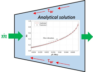
The analytical solutions of the conical pipes were validated by means of a comparison with numerical solutions of the same problems. The exact and numerical solutions in the validation tests were compared with reference to dimensionless variables Ma and fL/D(x), on the basis of the analysis made in §§ 3.2 and 3.3. Air was considered as the fluid in the tests (R = 287 J kg−1K−1, γ = 1.4).
Figure 2 reports a validation test for a convergent nozzle (dD/dx = const. < 0, c = −0.136), whereas figure 3 shows a validation test for a divergent conical nozzle (dD/dx = const. > 0, c = −0.373). The analytical solutions are plotted with a continuous line and were calculated by applying (3.22), whereas the numerical solutions are plotted with circle symbols and were computed by discretising (3.6) with a classical fourth-order Runge–Kutta method for initial value ODE problems (Hairer, Norsett & Wanner Reference Hairer, Norsett and Wanner1993; Butcher Reference Butcher2016) and by using (3.1) at the computational nodes for the calculus of the temperature  $(Ma = u/\sqrt {\gamma RT} )$.

Figure 2. Validation test for the exact solution with reference to a conical convergent nozzle. Test conditions: L = 45 cm, D 1 = 8 cm, D 2 = 3.5 cm,  $p_1^0 = 5\;\textrm{bar}$, T 0 = 500 K, Ma 1 = 0.11, f = 4⋅10−3, γ = 1.4, R = 287 J kg−1K−1, Δx = 0.5 mm
  $(\dot{m} = 0.857\;\textrm{kg}\;{\textrm{s}^{ - 1}})$.

Figure 3. Validation test for the exact solution with reference to a conical divergent nozzle. Test conditions: L = 60 cm, D 1 = 5 cm, D 2 = 9 cm,  $p_1^0 = 2\;\textrm{bar}$, T 0 = 400 K, Ma 1 = 1.1, f = 6⋅10−3, γ = 1.4, R = 287 J kg−1K−1, Δx = 0.5 mm
  $(\dot{m} = 0.787\;\textrm{kg}\;{\textrm{s}^{ - 1}})$.
Figure 4 refers to a validation test for the  $\textrm{d}D/\textrm{d}x = 4\gamma\,f/(3 - \gamma)\;\textrm{case}$ (cf. § 3.3): the exact solution of the nozzle was calculated with (3.28), whereas the numerical solution was obtained as in figures 2 and 3.

Figure 4. Validation test for the exact solution for the  $\textrm{d}D/\textrm{d}x = 4\gamma f/(3 - \gamma )$ case. Test conditions: L = 40 cm, D 1 = 6 cm, D 2 = 9 cm,
  $p_1^0 = 2\;\textrm{bar}$, T 0 = 400 K, Ma 1 = 1.1, f = 0.0214, γ = 1.4, R = 287 J kg−1K−1, Δx = 0.5 mm
  $(\dot{m} = 1.134\;\textrm{kg}\;{\textrm{s}^{ - 1}})$.
The flow direction, along which x grows from 0 to L, is indicated with an arrow in each graph. The uniform values of f reported in the captions were calculated by means of a Moody diagram: the Reynolds numbers were evaluated with the assigned boundary data (a value of μ has to be estimated for the air), and feasible relative roughness values were assumed.
The performed tests show an excellent agreement between the corresponding curves, and this is clear proof of the physical consistency of the proposed solutions for the  $\textrm{d}D/\textrm{d}x = cost$ cases.
As far as physical representativeness is concerned, the Mach number is related to flow compressibility, whereas fL/D is related to the nozzle geometry and friction. The percentage variation of Ma over the nozzle is higher than or equal to that of fL/D(x) and this means that the Mach number is sensitive to changes in this parameter. A Matr Mach number is also evaluated, based on the transverse flow velocity, which is assumed to be  ${u_{tr}}\sim u \cdot \tan (\alpha /2)$, where α is the conical opening angle of the pipe. This secondary Mach number can be used as a dimensionless factor to take into account the order of magnitude of the 2-D effects. Both Ma 2, which appears as the dependent variable in (3.22) and (3.28), and fL/D(x) feature higher orders of magnitude than
  $Ma_{tr}^2$ (
 $Ma_{tr}^2 \lt 0.0025$ with data in figure 2,
  $Ma_{tr}^2 \lt 0.0054$ with data in figure 3 and
  $Ma_{tr}^2 \lt 0.0034$ with data in figure 4) and this guarantees the accuracy of the obtained results compared to 2-D simulations. In particular, since the
  $Ma_{tr}^2$ values are much lower than the corresponding ones for fL/D(x), friction have more influence than the 2-D effects that have been neglected.
Furthermore, it is verified that the longitudinal variation of the cross-section, namely (1/A)(dA/dx)Δx with Δx = 1 cm, is much smaller than unity in all cases, and the 1-D assumption is therefore also feasible considering the geometrical data (Kamm & Shapiro Reference Kamm and Shapiro1979).
The Mach number increases with the flow direction in figures 2–4: in figure 2 (subsonic motion), the effects of both wall friction and a reduction in D contribute to accelerating the flow, whereas the accelerating effect of the increasing D in figures 3 and 4 (supersonic motion) prevails over the decelerating effect of friction. As a result, the concavity of Ma is facing upwards in figure 2, while it is facing downwards in figures 3 and 4.
The velocity gradient, namely du/dx, is small when the slope of the Ma versus fL/D curve is small and enlarges when this curve becomes steep. The highest values of the velocity gradient are reached close to the sonic condition. In the test to which figure 2 refers, du/dx takes on the highest values at the exit of the conical pipe where the Mach number is at a maximum and is close to 0.91: in fact, it was shown, in § 4, that  $\textrm{d}u/\textrm{d}x \to \infty$ when
  $Ma \to {1^ - }$ in a conical convergent pipe. In the tests of figures 3 and 4,
  $\textrm{d}D/\textrm{d}x \gt f\gamma M{a^2}\,\forall x$, 0 ≤ x ≤ L, and the flow is initially supersonic, du/dx therefore progressively reduces in modulus as Ma progressively increases.
The accuracy of the estimation of the uniform friction coefficient used in the solutions could be improved by performing a second iteration. A space-averaged value of f over the conical nozzle could be evaluated, on the basis of the exact solutions obtained in figures 2–4 and of an adequate model of the friction coefficient, which could also consider compressibility effects, via the Mach number, in addition to the dependence on the Reynolds number and the relative roughness (Schwartz Reference Schwartz1987). The analytical solutions could then be recalculated with this more accurate value of f in order to refine the predictions.
Finally, figure 5 plots a validation test that refers to a divergent pipe (dD/dx = const. > 0, c = −0.31) under an off-design working condition. The flow is supersonic at the conical pipe inlet (Ma 1 > 1) and the design solution is completed with a dashed line. The off-design condition consists of pressure pE, which is higher than psh, 2 to obtain a normal shock within the pipe.

Figure 5. Validation test for the exact weak solution in the case of a normal shock. Test conditions: L = 60 cm, D 1 = 4 cm, D 2 = 9 cm,  $p_1^0 = 10\;\textrm{bar}$, T 0 = 400 K, Ma 1 = 1.05, f = 5⋅10−3, γ = 1.4, R = 287 J kg−1K−1, Δx = 0.25 mm
  $(\dot{m} = 2.534\;\textrm{kg}\;{\textrm{s}^{ - 1}})$.
The exact weak solution is obtained by means of an iterative procedure. The shock position is initially assumed at a certain abscissa xsh, and (3.22) is used to calculate Ma(x) in the 0 ≤ x ≤ xsh interval. The value of the Mach number upstream of the shock, namely Maup,sh = Ma(xsh), is applied to (4.3) in order to evaluate Mado,sh (cf. also figure 5). The latter is then used as a boundary datum to calculate the analytical solution in the xsh ≤ x ≤ L interval by means of (3.22). Finally, the value of the pressure at the final section of the conical pipe is determined using (3.22) at x = L, and (3.1) and (3.3). If such a tentative pressure were equal to pE, the exact solution hypothesised for Ma(x) would be the right one. Instead, if this was not the case, the xsh position of the shock will be modified and iterations will be repeated until the pressure at the final section of the nozzle is equal to pE within a prescribed tolerance.
Unlike figures 2–4, the numerical solution was not obtained from the discretisation of (3.6), due to the presence of a shock. The unsteady Euler PDEs, namely (2.1) with  ${\dot{q}_f} = 0$ and (2.2), were discretised, and their time-asymptotic numerical space distributions were plotted with the symbols shown in figure 5. The implemented PDE solver was a conservative method, based on a flux vector splitting technique, which applied a high-resolution upwind discretisation scheme with a Van Leer flux limiter (Toro Reference Toro2009). The value of Δx was selected in order to guarantee a grid independent numerical solution and the time step, namely Δt, was set to obtain σ = 0.9, where
  $\sigma = |u + \sqrt {\gamma RT} {|_{max}}\mathrm{\Delta }t/\mathrm{\Delta }x$ is the instantaneous Courant number (Toro Reference Toro2009) and
  $|u + \sqrt {\gamma RT} {|_{max}}$ is the maximum modulus of the
  $u(x,t) + \sqrt {\gamma RT(x,t)}$ numerical space distribution at each fixed time instant.
As can be inferred, the exact weak solution in figure 5 also coincides perfectly with the corresponding numerical solution. This exact solution represents an almost unique case in which the Euler equations, written for a compressible flow in a pipe with a variable cross-section and wall friction, can be solved in the presence of a shock. Such a solution can be used to compare the performance of various conservative numerical schemes in the simulation of the shocks that occur in conical nozzles.
6. Conclusions
In this paper, new analytical solutions are obtained for the quasi-one-dimensional steady-state compressible viscous adiabatic flow of an ideal gas through a conical nozzle or a diffuser. These solutions are valid for both subsonic and supersonic continuous flows as well as for discontinuous flows and extend the set of gas dynamics analytical solutions that are currently available.
The original set of nonlinear generalised Euler ODEs for the quasi-one-dimensional steady-state compressible flow with wall friction is reduced to a single, nonlinear, homogeneous Abel ODE of the first kind with variable coefficients. In order to obtain an ODE that can be solved analytically, it is essential to determine the exact transformations of the variables and to identify the kinetic energy per mass unit as the physical dependent variable that appears in the final ODE of the problem. Furthermore, the conditions required to analytically solve the canonical form of the Abel ODE must be satisfied, and such conditions can lead to constraints on the pipe diameter, which is only allowed to vary linearly with x.
The obtained exact solutions have been then represented in non-dimensionless form. The Mach number, the f L/D factor and γ are identified as the fundamental groups of the dimensionless solutions. The order of magnitudes of Ma 2 and f L/D are much larger than that of  $Ma_{tr}^2$ and this proves that friction plays a more significant role than the neglected 2-D effects.
A fundamental differential equation, which relates the driving factors of the flow evolution, that is, nozzle diameter variation and friction, to the Mach number and the logarithmic derivative of the velocity along the nozzle, is derived and then discussed to interpret the exact solutions. A critical flow (Ma = 1) can only be reached along a general divergent nozzle, at a section where  $\textrm{d}D/\textrm{d}x = f\gamma$. A choking condition is highlighted for conical divergent nozzles: if the viscous flow is initially subsonic, the flow cannot be accelerated to a supersonic condition. A divergent nozzle with variable
  $\textrm{d}D/\textrm{d}x$ must be designed to overcome this limitation.
When the pressure in the environment downstream of a conical divergent nozzle, fed with a supersonic flow, is sufficiently higher than the pressure design value, as calculated by means of the continuous exact solution, a normal shock can occur inside the nozzle and, hence, the continuous exact solution does not hold. An exact iterative weak solution of the flow, based on Rankine–Hugoniot conditions, has been obtained for this case and the conditions of existence of such a weak solution have been specified.
Finally, the obtained exact solutions have been successfully validated through a comparison with the corresponding numerical solutions of the generalised Euler equations. The validated solutions can be used for several technological applications and the exact weak solution may serve as a reference term, in computational fluid dynamics, to evaluate the performance of conservative schemes.
Declaration of interests
The author reports no conflict of interest.


