


1 Introduction
Cavities are common features of air or water flows in industrial and environmental applications which can exhibit various shapes, sizes and configurations. Still, they are often simplified as rectangular dead-zones connected through one face to an established one-dimensional flow. Cavities have been extensively studied for acoustic and aeronautic purposes, mostly dealing with aircraft sound generation (Hussain & Zaman Reference Hussain and Zaman1978; Selfridge, Reiss & Avital Reference Selfridge, Reiss and Avital2017). In riverine environments, typical lateral cavities with a free surface are harbours, oxbow lakes or sheltered zones downstream of boulders (Sanjou & Nezu Reference Sanjou and Nezu2013; Jackson, Apte & Haggerty Reference Jackson, Apte and Haggerty2015; Sandoval et al. Reference Sandoval, Mignot, Mao, Bolster and Escauriaza2019). These sheltered zones favour the development of fauna and flora and thus play a major role for ecosystems. Moreover, gravity waves can resonate in such cavities, producing large oscillations of the free surface, usually called ‘seiche’, and may disable the loading of ships in harbours (Kimura & Hosoda Reference Kimura and Hosoda1997).
For any type of cavity, a mixing layer develops at the interface between the cavity and the main flow. Given the strong velocity gradient across the mixing layer, Kelvin–Helmholtz instability develops into coherent vortices, generated in the upstream region of the mixing layer and advected downstream (Raupach, Finnigan & Brunet Reference Raupach, Finnigan and Brunet1996; Charru Reference Charru2007). Rockwell & Knisely (Reference Rockwell and Knisely1978) reported that in such a bounded mixing layer, vortices are highly coherent, which differs from what is typically encountered in convective mixing layers (Godreche Reference Godreche1998). Here the coherency is maintained all along the mixing layer, meaning no vortex pairing occurs. Consequently, the frequencies of vortex shedding (at the upstream edge) and impingement (at the downstream edge) are equal, and are referred to as ‘cavity frequencies’ in what follows.
In a riverine environment, the mixing layer governs momentum (Mignot, Cai & Riviere Reference Mignot, Cai and Riviere2019) and mass (Sanjou & Nezu Reference Sanjou and Nezu2013) exchanges between the cavity and the main stream as well as the free-surface oscillation (Meile, Boillat & Schleiss Reference Meile, Boillat and Schleiss2011). Knowledge of the cavity frequency is thus crucial for the management of cavity flows. Cavities without a free surface, where only pressure waves travel, are defined as ‘acoustic cavities’. Their behaviour is very similar to that of open-channel cavities where gravity waves propagate with a much higher energy. Despite their similarities, they exhibit key differences.
In acoustics, the cavity frequency depends on the Mach number ( $M=U/c_{p}$), which compares the flow velocity
  $U$ to the pressure wave celerity
  $c_{p}$. For low Mach numbers (
 $M<0.2$), the cavity frequency is governed by the natural frequency of the cavity, whereas for high Mach numbers (
 $M>0.2$), it is governed by a feedback loop between vortices and pressure waves (Rossiter Reference Rossiter1964). Moreover, several frequencies can coexist at the same time, for a fixed Mach number (Larcheveque et al. Reference Larcheveque, Sagaut, Mary, Labbe and Comte2003).
In open-channel cavities, Wolfinger, Ozen & Rockwell (Reference Wolfinger, Ozen and Rockwell2012) recently measured the evolution of this frequency with the Froude number of the main stream. The Froude number,  $F=U/c$, compares the flow velocity
  $U$ to the gravity wave celerity
  $c$, similar to the Mach number for acoustic cavities. In this case though, the vortex shedding frequency is ‘locked on’ a natural frequency of the cavity and the frequency remains constant for high Froude numbers (
 $0.6<F<1$). For lower Froude numbers (
 $F<0.6$), the frequency increases with the Froude number. Moreover, Wolfinger et al. (Reference Wolfinger, Ozen and Rockwell2012) reveal that only one frequency is observed for a given flow (with sometimes its first harmonic). These results exhibit an opposite behaviour between acoustic and open-channel cavities. The authors then proposed an experimental linear trend of the oscillation frequency as a function of the Froude number. Even though a feedback loop was mentioned for a riverine environment (Tsubaki & Fujita Reference Tsubaki and Fujita2006), no analytical prediction of the oscillation frequency has been proposed to the best of our knowledge. Hence, it remains unknown if the frequencies measured by Wolfinger et al. (Reference Wolfinger, Ozen and Rockwell2012) correspond to a feedback loop similar to the one measured and modelled in acoustic cavities. The major difference lies in the different types of feedback waves: pressure waves for acoustic cavities and gravity waves in open channels.
The aim of the present work is to take advantage of the existing knowledge available in the area of acoustic cavities to explain and model the surface oscillation and vortex frequencies in open-channel cavities. Section 2 recalls the theory for the feedback model applied to acoustic cavities and proposes an adaptation for open-channel conditions. Section 3 introduces the experimental set-up used for the validation as well as the measurement techniques employed herein. Finally § 4 presents the capabilities of the model in predicting the cavity frequency for open-channel cavities, followed by a conclusion in § 5.
2 Theoretical model for vortex frequency
2.1 Model for frequency prediction in acoustics
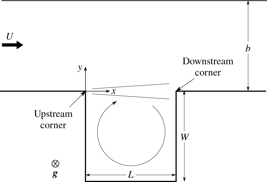
Figure 1. Experimental set-up (top view).
As introduced in § 1, the analytical model predicting the cavity frequency in acoustics relies on the natural frequency for low Mach numbers and on the feedback loop in the mixing layer for high Mach numbers.
The natural frequency of an acoustic cavity can be computed by simplifying it as a rectangular enclosure with fluid at rest (Plumbee, Gibson & Lassiter Reference Plumbee, Gibson and Lassiter1962). This frequency is ‘natural’ as it is an intrinsic property of the cavity, and does not depend on the adjacent flow. Cavity-type oscillations, induced by compressibility effects, can also be computed using the Helmholtz resonator theory.
For the feedback loop, the model considers the following events. As a vortex is shed (near the upstream corner of the cavity, denoted by subscript  $v$, with a phase
  $\unicode[STIX]{x1D6F7}_{v}$), it is advected by the flow and impinges the downstream corner. There, it generates a local pressure variation (following the Bernoulli principle) inducing a pressure wave (denoted by subscript
  $p$, with a phase
  $\unicode[STIX]{x1D6F7}_{p}$) with the same frequency as that of the vortex shedding, which propagates in every direction, including upwards, i.e. towards the upstream corner of the cavity. The model assumes that the selected frequency is the one that fulfils the resonant conditions. This implies that the phase difference
  $\unicode[STIX]{x0394}\unicode[STIX]{x1D6F7}=\unicode[STIX]{x1D6F7}_{v}-\unicode[STIX]{x1D6F7}_{p}$, where
  $v$ and
  $p$ refer to vortex and pressure waves (see figure 1) at the upstream corner, satisfies
 $$\begin{eqnarray}\unicode[STIX]{x0394}\unicode[STIX]{x1D6F7}(x=0)=2N\unicode[STIX]{x03C0},\end{eqnarray}$$
 with  $N$ being an integer (
 $N=1,2,3,\ldots$). Using the definition of the wavelength
  $\unicode[STIX]{x1D706}=c/f$, with
  $c$ the celerity of waves and
  $f$ their frequency, this reads
 $$\begin{eqnarray}N=\frac{L}{\unicode[STIX]{x1D706}_{v}}+\frac{L}{\unicode[STIX]{x1D706}_{p}}.\end{eqnarray}$$
 Integer  $N$ can be seen as the number of vortices plus pressure wave wavelengths along the cavity–main flow interface (
 $x=0$ to
  $L$). Using
  $f=c_{v}/\unicode[STIX]{x1D706}_{v}=c_{p}/\unicode[STIX]{x1D706}_{p}$, this reads
 $$\begin{eqnarray}N=\frac{Lf}{c_{v}}+\frac{Lf}{c_{p}},\end{eqnarray}$$
or alternatively, introducing the Strouhal number
 $$\begin{eqnarray}St=\frac{f\,L}{U}=\frac{N}{\displaystyle \frac{U}{c_{v}}+\frac{U}{c_{p}}},\end{eqnarray}$$
 with  $U$ the velocity of the main stream. The value of the ratio
  $R_{v}=c_{v}/U$ is usually measured experimentally, and
  $R_{v}$ has been reported as ranging between
  $0.35$ (East Reference East1966) and
  $0.625$ (Rowley et al. Reference Rowley, Williams, Colonius, Murray and Macmynowski2006). Rossiter (Reference Rossiter1964) states that
  $R_{v}=0.57$, which is the standard value used in the literature.
For a given flow configuration, this model allows an infinity of solutions, with  $N=1,2,3$, etc. Rossiter (Reference Rossiter1964) and subsequent authors compared the frequency predicted by this model with experimental data and noticed a systematic shift. Most of them thus introduce a correction factor,
  $\unicode[STIX]{x0394}N$ with
  $N^{\prime }=N+\unicode[STIX]{x0394}N$, attributed to ‘a constant phase lag corresponding to a time delay between the vortex arrival at the impingement corner and the emission of the acoustic pulse’ (Gloefert Reference Gloefert2009). The corrected model then reads
 $$\begin{eqnarray}\frac{f\,L}{U}=\frac{N+\unicode[STIX]{x0394}N}{\displaystyle \frac{1}{R_{v}}+M}.\end{eqnarray}$$
 Empirical values for  $\unicode[STIX]{x0394}N$, proposed by successive authors, exhibit a large variation, from
  $\unicode[STIX]{x0394}N=-0.58$ (Rossiter Reference Rossiter1964) to
  $\unicode[STIX]{x0394}N=0.5$ (Sarohia Reference Sarohia1977). A global three-dimensional stability analysis of the mixing layer (Bilanin & Covert Reference Bilanin and Covert1973; Alvarez, Kerschen & Tumin Reference Alvarez, Kerschen and Tumin2004), injecting the resonant condition, leads to a similar result. Note that the celerity of the pressure wave does not take into account the local flow velocity as it is supposed to travel in the cavity, where the mean velocity is negligible. The fact that the model applies to supersonic flows (
 $M>1$) supports this hypothesis, as the wave could not propagate upstream otherwise.
2.2 Transposition to open-channel configurations
We expect that the oscillation frequency of open-channel cavities is governed by the same two phenomena. They are transposed to the open-channel configuration in the following subsections.
2.2.1 Natural frequencies of open-channel cavities
The natural modes of a closed rectangular water volume at rest were initially introduced by Lamb (Reference Lamb1945) and recently reviewed by Rabinovitch (Reference Rabinovitch2009). These modes can be aligned with one or both cavity axes  $x$ and
  $y$ (see table 1). The corresponding frequencies are denoted
  $f_{n_{x}n_{y}}$ with
  $n_{x}$ and
  $n_{y}$ the number of nodes along axes
  $x$ and
  $y$, respectively. In a rectangular basin of dimensions
  $l_{x}$ (along axis
  $x$) and
  $l_{y}$ (along axis
  $y$), the natural frequencies then read
 $$\begin{eqnarray}f_{n_{x}n_{y}}=\frac{c}{2}\left[\left(\frac{n_{x}}{l_{x}}\right)^{2}+\left(\frac{n_{y}}{l_{y}}\right)^{2}\right]^{1/2},\end{eqnarray}$$
 with  $c$ the celerity of gravity waves in still water (Stocker Reference Stocker1957):
 $$\begin{eqnarray}c=\frac{g}{2\unicode[STIX]{x03C0}f}\tanh \frac{2\unicode[STIX]{x03C0}\overline{h}f}{c},\end{eqnarray}$$
 where  $\overline{h}$ is the time-averaged water depth in the cavity and
  $f$ the frequency of the gravity wave. Note that this expression can reduce to the classical Merian (Reference Merian1828) expression for shallow conditions (
 $\unicode[STIX]{x1D706}\gg \overline{h}$) if
  $n_{x}=1$,
  $n_{y}=0$ and
  $c$ is simplified to
  $c=\sqrt{g\overline{h}}$. Following the notation of Wolfinger et al. (Reference Wolfinger, Ozen and Rockwell2012) and Tuna, Tinar & Rockwell (Reference Tuna, Tinar and Rockwell2013),
  $f$ can be normalized by
  $f_{10}=c/2L$, the natural frequency of the cavity corresponding to the first longitudinal mode (along
  $x$) with one node (see table 1):
 $$\begin{eqnarray}\frac{f_{n_{x}n_{y}}}{f_{10}}=\left[n_{x}^{2}+\left(n_{y}\frac{l_{x}}{l_{y}}\right)^{2}\right]^{1/2}.\end{eqnarray}$$
 Table 1 plots schematic views of three observed modes of the cavity and indicates the link between  $l_{x}$,
  $l_{y}$ and
  $W$,
$W$,  $b$,
$b$,  $L$ that depends on the cavity mode considered.
Table 1. Three amongst the most common natural frequencies of a rectangular open-channel cavity.

2.2.2 Feedback model adapted to open-channel cavities
When applied to open-channel lateral cavities, the feedback model relies on the same processes as for acoustic cavities with a gravity wave instead of a pressure wave. In the axis frame linked to the cavity (see figure 1), this gravity wave travels upstream at a celerity  $c$. As for the acoustic model, we assume here that: (1) both vortex and gravity waves are periodic with the same frequency
  $f$ and (2) they are in phase at both corners so that equations (2.3) and (2.5) still hold:
 $$\begin{eqnarray}N=\frac{Lf}{c_{v}}+\frac{Lf}{c}.\end{eqnarray}$$
Following the same normalization as for equation (2.8) and including the correction factor, the feedback frequency reads
 $$\begin{eqnarray}\frac{f}{f_{10}}=\frac{2F(N+\unicode[STIX]{x0394}N)}{\displaystyle \frac{1}{R_{v}}+F}.\end{eqnarray}$$
Again, equation (2.10) produces an infinity of solutions.
3 Experiments
3.1 Experimental campaign
Measurements aiming at validating the analytical model were performed at INSA-Universite de Lyon in a set-up similar to that used by Mignot et al. (Reference Mignot, Cai, Launay and Escauriaza2016). It consists of a 4.80 m long and  $b=30~\text{cm}$ wide open channel connected at mid-length to an adjacent rectangular lateral cavity. The channel and the cavity are horizontal, of rectangular section with glass bottom and sidewalls, with no step at the connection. At the channel inlet, the water overflows from the tank to the upstream branch of the channel through a converging section. Moreover, honeycomb meshes straighten the flow. At the outlet, a sharp crested weir adjusts the time-averaged water depth
  $\overline{h}=5.8~\text{cm}$ at the connection with the cavity. The flow finally recirculates in a closed loop and the corresponding flow rate is measured by an electromagnetic flow meter (ProMag50, Endress Hauser) with an uncertainty of
  $\pm 0.05~\text{l}~\text{s}^{-1}$. The length of the cavity (in the direction parallel to the channel) is fixed at
  $L=0.3~\text{m}$ and its width
  $W=0.5~\text{m}$.
According to a dimensional analysis, the oscillation frequency depends on three parameters:  $W/L$,
  $b/L$ and
  $F$. The strategy proposed herein is to keep
  $W/L$ and
  $b/L$ constant while varying the Froude number from
  $F=0.33$ to
  $0.65$, corresponding to the range of Froude numbers for which Wolfinger et al. (Reference Wolfinger, Ozen and Rockwell2012) reported an increasing cavity frequency (for
  $0.3<F<0.6$) followed by a lock-on regime (i.e. a linearly constant oscillation frequency value for
  $0.6<F<0.85$). Unfortunately, due to experimental constraints, the Froude number could not be increased beyond 0.65 for the present experimental device. In order to avoid any hysteresis effect, each configuration is initiated with the cavity flow at rest and measurements start after the water-level oscillations at the downstream corner reach a steady state.
3.2 Measurement methods
Three types of measurements are considered herein, using three different methods. The oscillation of the free surface near the downstream corner of the interface (figure 1) is measured using an ultrasonic probe, UNDK 20I6912 S35A from Baumer Electric AG (resolution  $\unicode[STIX]{x1D6FF}h\leqslant 0.3~\text{mm}$), with a sampling frequency equal to 200 Hz. Data are recorded during 10 min. Secondly, the two-dimensional horizontal velocity field, and associated vortex dynamics, in the region surrounding the interface is measured using particle image velocimetry. A 1 mm thick horizontal laser sheet is used to illuminate a horizontal plane across the mixing layer at
  $z/\overline{h}=0.8$. The images are recorded from underneath the flume, using an AV Manta G-235B camera,
  $1936\times 1216$ pixels with a spatial resolution of 0.3 mm per pixel. For each flow configuration, 33.3 s are recorded at a sampling frequency of 60 fps (2000 images). Finally, the two-dimensional free-surface deformation is measured using a fringe pattern projection method adapted from Takeda, Ina & Kobayashi (Reference Takeda, Ina and Kobayashi1981) and Przadka et al. (Reference Przadka, Cabane, Pagneux, Maurel and Petitjeans2011). A video projector, located 1.5 m above the free surface, projects vertically (downward) on the free surface a known fringe pattern image. The oscillation of the free surface then deforms the pattern so that the water depth displacement is computed at each pixel on each image by extracting the phase difference between the deformed and reference patterns. The post-processing finally applied is adapted from Aubourg (Reference Aubourg2006). In the end, for each flow configuration, the frequency of vortex shedding and free-surface oscillation is measured using three different methods, on three different days as these measurement techniques could not be applied simultaneously. The fair agreement between these frequencies gives confidence in the reproducibility and precision of the methods.
4 Results
4.1 Determination of  $R_{v}$ in open-channel cavities

The feedback model (2.10) requires one to estimate  $R_{v}=c_{v}/U$. The evolution of
  $R_{v}$ with the Froude number is plotted in figure 2(b),
  $c_{v}$ being obtained by averaging the travelling time of 40 consecutive vortices along the interface of the cavity, using the methodology proposed by Mignot et al. (Reference Mignot, Cai, Launay and Escauriaza2016). Ratio
  $R_{v}$ appears to remain constant with
  $F$:
$F$:  $R_{v}=0.56$ is in good agreement with the value reported by Rossiter (Reference Rossiter1964) (
 $R_{v}=0.57$) for acoustic cavities.

Figure 2. Dependence of the mixing layer dynamics on Froude number. (a) Ratio of interface flow velocity to bulk velocity with respect to Froude number. (b) Ratio of vortex velocity to bulk velocity with respect to Froude number.
4.2 Experimental validation of the model
Figure 3(a) plots the first three solutions of the feedback model (2.10) as solid lines, for  $N=1,2$ and
  $3$, here without correction (
 $\unicode[STIX]{x0394}N=0$), as well as data from Wolfinger et al. (Reference Wolfinger, Ozen and Rockwell2012) as red squares. It shows that these data closely match the mode
  $N=2$ of the feedback model, suggesting that the apparently linear trend observed by Wolfinger et al. (Reference Wolfinger, Ozen and Rockwell2012) for
  $F<0.6$ corresponds actually to the second feedback mode of the mixing layer. Figure 3(a) additionally plots the natural frequencies of the cavity, equation (2.8), as dashed horizontal lines. As already observed by Kegerise (Reference Kegerise1999), feedback and natural frequencies exhibit several matches for different Froude numbers. The selected frequencies are thus expected to fit, at best, these matches.
Free-surface oscillation frequencies from ultrasound measurements at the impingement corner are finally included in figure 3(a) (green symbols) for Froude numbers ranging from 0.3 to 0.65. While the frequencies measured by Wolfinger et al. (Reference Wolfinger, Ozen and Rockwell2012) linearly increase with the Froude number for  $F<0.6$, the present frequencies exhibit a different trend, divided in three ranges of Froude numbers.

Figure 3. Experimental validation of the feedback model. (a) Evolution of normalized frequency of free-surface oscillation with respect to Froude number. Red squares are data from Wolfinger et al. (Reference Wolfinger, Ozen and Rockwell2012). Solid lines are the three first modes ( $N=1,2,3$) of the model with
  $\unicode[STIX]{x0394}N=0$ obtained as best fitting. Dashed lines correspond to natural frequencies of the cavity. (b–d) Snapshots of the normalized free-surface oscillation
  $\unicode[STIX]{x1D702}^{\ast }=\unicode[STIX]{x1D702}/U^{2}/2g$; black zones are measurement noise due to direct light reflection.
First, for  $0.33<F<0.4$, the measured frequencies remain about constant at a value corresponding to mode
  $f_{02}$ and close to the feedback mode
  $N=2$ (2.10). To check the free-surface oscillation mode, figure 3(b) plots a snapshot of the free-surface deformation, obtained by fringe pattern projection, for the flow configuration with
  $F=0.35$. It reveals two wave crests along the cavity (
 $y=-W$) and main channel (
 $y=b$) walls, a trough at mid-length and two nodes depicted as white lines aligned along the
  $x$ axis. This confirms the natural mode associated with
  $f_{02}$ (table 1). Note that a similar pattern is retrieved for all configurations with
  $F<0.4$, so that the corresponding symbols in figure 3(a) are plotted as triangles. The plateau reveals that the cavity oscillation frequency is locked on a natural mode of the cavity. Furthermore, it is possible to estimate the experimental value of
  $N$, denoted
  $N_{e}$, using (2.9) (where
  $f$,
$f$,  $U_{i}$ and
  $c_{v}$ are measured as described above):
  $N_{e}=[2.08,2.32]$ agrees fairly well with the expected mode
  $N=2$ giving confidence in the validity of the feedback model.
Similarly, for  $0.4<F<0.48$, the frequencies are close to
  $f_{11}$ and to the feedback mode
  $N=3$ (2.10). The snapshot of the free-surface deformation for
  $F=0.45$ (figure 3c) reveals a chessboard pattern, with two crests: one at the upstream corner of the cavity and one at the opposite corner (
 $x=L$,
  $y=-W$); and two troughs: one at the downstream corner of the interface and the other at the opposite corner (
 $x=0$,
  $y=-W$). The two nodes are aligned along
  $x$ and
  $y$ axes. This
  $f_{11}$ mode is retrieved for all configurations with
  $0.4<F<0.48$, and the corresponding symbols in figure 3(a) are plotted as circles. For this second plateau, the cavity oscillation frequency is locked on a second natural mode of the cavity. Moreover,
  $N_{e}=[2.80,3.16]$ agrees with the expected feedback mode
  $N=3$.
Finally, for  $0.48<F<0.65$, frequencies are close to feedback mode
  $N=3$ and near the natural mode
  $f_{10}$. This third plateau corresponds to a third lock-on, similar to that reported by Wolfinger et al. (Reference Wolfinger, Ozen and Rockwell2012) but starting at a lower value of Froude number: namely
  $F\approx 0.48$ instead of
  $F\approx 0.6$, reported by those authors. The snapshot of the free-surface deformation for
  $F=0.55$ (figure 3d) shows one crest and one trough along the lateral walls of the cavity and one node in between. This confirms that the free-surface deformation corresponds to
  $f_{10}$ mode. A similar tendency is retrieved for all configurations with
  $0.48<F<0.6$ and the symbols are plotted as stars in figure 3(a). Also,
  $N_{e}=[1.99,2.03]$ agrees with the expected feedback mode
  $N=2$.
To summarize, the peak frequencies of the cavity oscillation are distributed among three lock-on plateaus, which correspond to close matches between a feedback mode in the mixing layer (but with less agreement for the third plateau) and a natural mode of the cavity for the free-surface deformation. Still, other matches between feedback modes (2.10) and natural modes (2.8) could have been selected for several flow configurations. For instance, natural mode  $f_{10}$ and feedback mode
  $N=3$ match for
  $F\approx 0.35$ (figure 3a) while the observed mode corresponds to a match of
  $f_{02}$ and
  $N=2$. The mode selection in this case is thus still an open question at this stage.
5 Conclusion
The present paper deals with open-channel cavity flows for incoming Froude numbers ranging from 0.33 to 0.65. It is shown that the processes governing vortex shedding substantially differ from those of classical free mixing layers. This difference is due to the interaction of the vortex shedding with the gravity waves of two different kinds that are encountered in the flow. Waves of the first kind are standing waves. They correspond to the natural modes of the cavity and their frequencies are well predicted by classical equations. Waves of the second kind are the feedback gravity waves. They propagate against the current and their frequencies are well predicted by the so-called feedback model developed in this work, taking inspiration from acoustic cavity models. In this study, the interactions are always observed jointly with the two types of waves. In other words, the frequency of the vortex shedding always matches with a common solution to the two models. However, for a given Froude number, several common solutions exist.
The selection of the resonant mode may result from the different values of damping of each available natural mode of the cavity. An attempt to estimate these damping rates could be made through a numerical stability analysis. Another process that selects the resonant mode could be another feedback process (other than the Rossiter modes), related to the motion of vortices along the recirculation cell inside the cavity. This cell can indeed trap vortices near the impingement edge of the cavity, make them rotate along the cavity walls and reintroduce them at the upstream edge (Mignot & Brevis Reference Mignot and Brevis2019), where they could interact with the vortex shedding process. The selection of the actual resonant mode of the cavity is thus still an open question, which should be addressed in future works.
Acknowledgements
This work was performed under the framework of PHC-Tournesol 2018-40633YJ. The authors are grateful to L. Engelen and T. De Mulder from the University of Ghent for fruitful discussions.
Declaration of interests
The authors report no conflict of interest.


