INTRODUCTION
This paper focuses on the demand for money in the United States, building on a large body of recent literature, which Barnett (1997) calls the “high road” literature, that takes a microeconomic and aggregation-theoretic approach to the demand for money. This literature follows the innovative works by Chetty (1969), Donovan (1978), and Barnett (1980, 1983) and utilizes the demand systems approach to investigating the interrelated problems of monetary aggregation and estimation of monetary asset demand functions—see, for example, Ewis and Fisher (1984, 1985), Serletis and Robb (1986), Serletis (1991), Fisher and Fleissig (1994, 1997), Fleissig and Serletis (2002), and Serletis and Shahmoradi (2005) among others.
These works are interesting and attractive, as they include estimates of the demand for money and of the degree of substitutability between money and near-monies using locally flexible functional forms [see Ewis and Fisher (1984), Serletis and Robb (1986), and Serletis (1991)], effectively globally regular functional forms [see Barnett (1983)], and globally flexible functional forms [see Ewis and Fisher (1985), Fleissig and Serletis (2002), and Serletis and Shahmoradi (2005)]. Research has indicated that the simple-sum approach to monetary aggregation cannot be the best that can be achieved, in the face of cyclically fluctuating incomes and interest rates.
The usefulness of flexible functional forms, however, depends on whether they satisfy the theoretical regularity conditions of positivity, monotonicity, and curvature, and in this literature there has been a tendency to ignore regularity. In fact, as Barnett (2002, p. 199) put it in his Journal of Econometrics Fellow's opinion article, without satisfaction of all three theoretical regularity conditions,
the second-order conditions for optimizing behavior fail, and duality theory fails. The resulting first-order conditions, demand functions, and supply functions become invalid.
Motivated by the widespread practice of ignoring the theoretical regularity conditions, as summarized in Table 1, as well as the practice of not reporting the results of full regularity checks, in this paper we revisit the demand for money in the United States in the context of five of the most widely used locally flexible functional forms, using recent state-of-the-art advances in microeconometrics. The flexible forms are the generalized Leontief [see Diewert (1974)], the translog [see Christensen et al. (1975)], the almost ideal demand system [see Deaton and Muellbauer (1980)], the Minflex Laurent [see Barnett (1983)], and the normalized quadratic reciprocal indirect utility function [see Diewert and Wales (1988)]. These forms provide the capability to approximate systems resulting from a broad class of generating functions and also to attain arbitrary elasticities of substitution—although at only one point (that is, locally).

We pay explicit attention to all three theoretical regularity conditions (positivity, monotonicity, and curvature) and argue that much of the older monetary demand systems literature ignores economic regularity. We argue that unless regularity is attained by luck, flexible functional forms should always be estimated subject to regularity, as suggested by Barnett (2002) and Barnett and Pasupathy (2003). In fact, we follow Ryan and Wales (1998) and Moschini (1999) and treat the curvature property as a maintained hypothesis and build it into the models being estimated, very much like the homogeneity in prices and symmetry properties of neoclassical consumer theory.
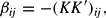
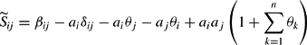
In particular, Ryan and Wales (1998) suggest a relatively simple procedure for imposing local curvature conditions. Their procedure applies to those locally flexible demand systems for which, at the point of approximation, the n×n Slutsky matrix S can be written as

where B is an n×n symmetric matrix, containing the same number of independent elements as the Slutsky matrix, and C is an n×n matrix whose elements are functions of the other parameters of the system. Curvature requires the Slutsky matrix to be negative semidefinite. Ryan and Wales (1998) draw on related work by Lau (1978) and Diewert and Wales (1987) and impose curvature by replacing S in equation (1) with −KK′, where K is an n×n lower triangular matrix, so that −KK′ is by construction a negative semidefinite matrix. Thus, solving explicitly for B in terms of K and C yields

meaning that the models can be reparameterized by estimating the parameters in K and C instead of the parameters in B and C. That is, we can replace the elements of B in the estimating equations with the elements of K and the other parameters of the model, thus ensuring that S is negative semidefinite at the point of approximation, which could be any data point.
Ryan and Wales (1998) applied their procedure to three locally flexible functional forms—the almost ideal demand system, the normalized quadratic, and the linear translog. Moreover, Moschini (1999) suggested a possible reparameterization of the basic translog to overcome some problems noted by Ryan and Wales (1998) and also imposed curvature conditions locally in the basic translog. More recently, Serletis and Shahmoradi (2007) build on Ryan and Wales (1998) and Moschini (1999) and impose curvature conditions locally on the generalized Leontief model. In doing so, they exploit the Hessian matrix of second-order derivatives of the reciprocal indirect utility function, unlike Ryan and Wales (1998) and Moschini (1999), who exploit the Slutsky matrix.
In this paper we show that even the imposition of the maintained hypothesis of local curvature is not sufficient for regularity with most locally flexible demand systems, because of curvature violations at other points within the region of the data, and also because of induced violations of monotonicity. We assess the effects of curvature violations on a model's ability to produce stable elasticity estimates and also argue that the current practice of correcting for serial correlation without reporting the results of monotonicity checks (even when the curvature conditions are imposed) is not justified, because serial correlation correction increases the number of curvature violations and also leads to induced violations of monotonicity with most models.
The paper is organized as follows. Section 2 briefly sketches the neoclassical problem facing the representative agent, and Section 3 discusses the five parametric flexible functional forms that we use in this paper, as well as relevant procedures for imposing curvature conditions to each of these forms. Section 4 is devoted to data and econometric issues, whereas in Section 5 we estimate the models, report on theoretical regularity violations, and explore the economic significance of the results. In Section 6 we assess the effects of curvature violations on a model's ability to produce stable elasticity estimates, whereas in Section 7 we investigate the effects on regularity of serial correlation corrections of dynamically misspecified models. The final section concludes the paper.
THE MONETARY PROBLEM
Following Serletis and Shahmoradi (2005), we assume that the representative money holder faces the problem
where x =(x1, x2, …, x8) is the vector of monetary asset quantities described in Table 2; p =(p1, p2, …, p8) is the corresponding vector of monetary asset user costs; and y is the expenditure on the services of monetary assets. It is to be noted that the existing theory of aggregation over economic agents is much more complicated than that for aggregation over goods and also independent of the theory of aggregation over goods. In fact, the theory discussed here on aggregation over assets for one economic agent remains valid for any means of aggregation over economic agents—see Barnett et al. (1992) or Barnett and Serletis (2000) for more details regarding this issue.

Because the functional forms that we use in this paper are parameter intensive, we face the problem of having a large number of parameters in estimation. To reduce the number of parameters, we follow Serletis and Shahmoradi (2005) and separate the group of assets into three collections based on empirical pretesting. Thus the monetary utility function in (2) can be written as

where the subaggregate functions fi(i=A, B, C) provide subaggregate measures of monetary services.
Although not the same, this structure of preferences is very similar to the one uncovered by Fisher and Fleissig (1994) and also used by Fleissig and Swofford (1996) and Fisher and Fleissig (1997) when they estimated their money demand models. Fisher and Fleissig (1994) found, using the NONPAR program of Varian (1982, 1983), that these groups of assets satisfy the weak separability condition for several generalized axiom of revealed preference (GARP)-consistent subperiods.
Instead of using the simple-sum index, currently in use by the Federal Reserve and most central banks around the world, to construct the monetary subbaggregates, fi(i = A, B, C), we follow Barnett (1980) and use the Divisia quantity index to allow for less than perfect substitutability among the relevant monetary components. In particular, the simple-sum index is Mt in

where
is the jth monetary component of the monetary aggregate Mt. This summation index views all components as dollar-for-dollar perfect substitutes.
The Divisia index (in discrete time) is defined as
according to which the growth rate of the aggregate is the weighted average of the growth rates of the component quantities, with the Divisia weights being defined as the expenditure shares averaged over the two periods of the change,
for j=1, …, n, where
is the expenditure share of asset j during period t, and
is the nominal user cost of asset j, derived in Barnett (1978),
which is just the opportunity cost of holding a dollar's worth of the jth asset. Above, p* is the true-cost-of-living index, rjt is the market yield on the jth asset, and Rt is the yield available on a benchmark asset that is held only to carry wealth between multiperiods.
LOCALLY FLEXIBLE FUNCTIONAL FORMS
In this section we briefly discuss the five functional forms that we use in this paper—the generalized Leontief, the basic translog, the almost ideal demand system, the Minflex Laurent, and the normalized quadratic reciprocal indirect utility function. These functions are all locally flexible and are capable of approximating any unknown function up to the second order.
The Generalized Leontief
The generalized Leontief (GL) functional form was introduced by Diewert (1973) in the context of cost and profit functions. Diewert (1974) introduced the GL reciprocal indirect utility function
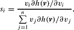
where v = [v1, v2, …, vn' is a vector of income normalized user costs, with the ith element being vi = pi/y, where pi is the user cost of asset i and y is the total expenditure on the n assets.
is an n × n symmetric matrix of parameters and a0 and ai are other parameters, for a total of (n2+3n+2)/2 parameters.
Using Diewert's (1974) modified version of Roy's identity,
where si=vixi and xi is the demand for asset i, the GL demand system can be written as
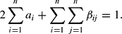
Because the share equations are homogeneous of degree zero in the parameters, we follow Barnett and Lee (1985) and impose the following normalization in estimation:
We follow Serletis and Shahmoradi (2007) and impose curvature conditions locally on the generalized Leontief model by building on Ryan and Wales (1998) and Moschini (1999). In doing so, we exploit the Hessian matrix of second-order derivatives of the reciprocal indirect utility function (3), unlike Ryan and Wales (1998) and Moschini (1999), who exploit the Slutsky matrix. In particular, because curvature of the GL reciprocal indirect utility function requires that the Hessian matrix be negative semidefinite, we impose local curvature (at the reference point) by evaluating the Hessian terms of (3) at v* = 1, as follows,
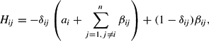
where δij is the Kronecker delta (that is,
when i=j and 0 otherwise). By replacing H by −KK′, where K is an n × n lower triangular matrix and K′ its transpose, the above can be written as

Solving for the ai and βij terms as a function of the
, we can get the restrictions that ensure the negative semidefiniteness of the Hessian matrix (without destroying the flexibility properties of (3), because the number of free parameters remains the same). In particular, when i≠j, equation (7) implies that
and for i=j it implies that
Substituting βij from (8) into the above equation, we get

or
which after some rearrangement yields
For the case of three assets (which is the case in our paper), conditions (8) and (9) imply the following six restrictions on (5):

where the kij terms are the elements of the K matrix.
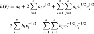
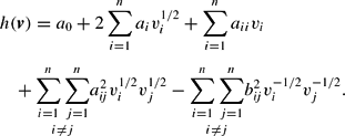
The Basic Translog
The basic translog (BTL) flexible functional form was introduced by Christensen et al. (1975). The BTL reciprocal indirect utility function can be written as

where
is an n×n symmetric matrix of parameters and a0 and ai are other parameters, for a total of (n2+3n+)/2 parameters.
The share equations, derived using the logarithmic form of Roy's identity,

are
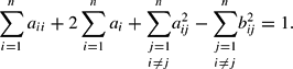
Applying the Ryan and Wales (1998) procedure for imposing local curvature to the basic translog, the Slutsky terms of (10) can be written as

for i, j=1, …, n, where δij is the Kronecker delta, as before. Ryan and Wales (1998) argued that in the case of the basic translog, replacing S by −KK′ is of little help in imposing local curvature, because the ijth element of
contains not just βij but also the terms
and
. As they noted, there are n(n+1)/2 independent βij parameters, but only n(n−1)/2 independent elements in
, rendering it no longer possible to express the βij terms in terms of the elements of K and of the other parameters of the model.
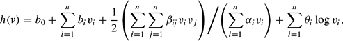
However, Moschini (1999) suggested a possible reparameterization of the basic translog to overcome the problem noted by Ryan and Wales (1998) so that we can still use their procedure for imposing local curvature in the BTL demand system. In particular, he showed that by letting
, we can rewrite (11) as

with sn given by
. With this parameterization, the Slutsky terms can be expressed in terms of a matrix of dimension (n−1)×(n−1), denoted by
, with the ijth element written as
for i, j=1, …, n−1. Note that now in equation (13) there are exactly n(n−1)/2
terms, as there are n(n−1)/2 βij terms.
By replacing
by
in (13), for n=3 we get the following three restrictions on (12),

where the kij terms are the elements of the
matrix.
The Almost Ideal Demand System
The almost ideal demand system (AIDS) is written in share equation form [see Deaton and Muellbauer (1980) for more details] as
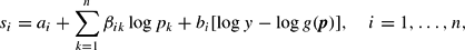
where log g(p) is a translog price index defined by
In equation (14), si is the ith budget share, y is income, pk is the kth price, and (a, b, β) are parameters of the demand system to be estimated. Symmetry (βij = βji for all i, j), adding up
, and homogeneity
for all i) are imposed in estimation. With n assets the AIDS model's share equations contain (n2 + 3n − 2)/2 free parameters.
Applying the Ryan and Wales (1998) procedure for imposing local curvature, we write the ijth element of the Slutsky matrix associated with the AIDS demand system, equation (14), at the point y=pk=1 (∀k) as

for i, j=1, …, n, where
when i=j and 0 otherwise. Thus, following Ryan and Wales (1998), local curvature can be imposed by replacing the elements of B in the estimating share equations with the elements of K and the other parameters, as follows, for the ijth element of B:

for i, j=1, …, n.
For n=3, equation (15) implies the following three restrictions on (14),

where the kij terms are the elements of the
matrix.
The Minflex Laurent
The Minflex Laurent (ML) model, introduced by Barnett (1983) and Barnett and Lee (1985), is a special case of the Full Laurent model also introduced by Barnett (1983). Following Barnett (1983), the Full Laurent reciprocal indirect utility function is
where a0, ai,
bi, and
are unknown parameters and vi denotes the income-normalized price, as before.
By assuming that bi=0, bii=0 ∀i, and
∀i, j and forcing the off-diagonal elements of the symmetric matrices
and
to be nonnegative, (16) reduces to the ML reciprocal indirect utility function,
Note that the off-diagonal elements of A and B are nonnegative, as they are raised to the power of 2.
By applying Roy's identity to (17), the share equations of the ML demand system are

Because the share equations are homogeneous of degree zero in the parameters, we follow Barnett and Lee (1985) and impose the following normalization in the estimation of (18):
Hence, there are

parameters in (17), but the n(n−1)/2 equality restrictions,
∀i, j, and the normalization (19) reduce the number of parameters in equation (18) to (n2+3n)/2.
As shown by Barnett (1983, Theorem A.3), (17) is globally concave for every v≥0 if all parameters are nonnegative, as in that case (17) would be a sum of concave functions. If the initially estimated parameters of the vector
and matrix
are not nonnegative, curvature can be imposed globally by replacing each unsquared parameter with a squared parameter, as in Barnett (1983).
The NQ Reciprocal Indirect Utility Function
Following Diewert and Wales (1988), the normalized quadratic (NQ) reciprocal indirect utility function is defined as
where b0, b=[b1, b2, …, bn],
, and the elements of the n×n symmetric matrix
are the unknown parameters to be estimated. It is important to note that the quadratic term in (20) is normalized by dividing through by a linear function,

and that the nonnegative vector of parameters
is assumed to be predetermined.
As in Diewert and Wales (1988), we assume that α satisfies
Moreover, we pick a reference (or base-period) vector of income-normalized prices, v*=1, and assume that the B matrix satisfies the following n restrictions:
Using the modified version of Roy's identity (4), the NQ demand system can be written as
Finally, as the share equations are homogeneous of degree zero in the parameters, we also follow Diewert and Wales (1988) and impose the normalization

Hence, there are n(n+5)/2 parameters in (23), but the imposition of the (n−1) restrictions in (22) and (23) reduces the number of parameters to be estimated to (n2+3n−2)/2.
The normalized quadratic reciprocal indirect utility function defined by (20), (21), and (22) will be globally concave over the positive orthant if B is a negative semidefinite matrix and
—see Diewert and Wales (1988, Theorem 3). Although curvature conditions can be imposed globally if the initially estimated B matrix is not negative semidefinite or the initially estimated θ vector is not nonegative, the imposition of global curvature destroys the flexibility of the NQ reciprocal indirect utility function. Because of lack of flexibility when curvature conditions are imposed globally, here we follow Ryan and Wales (1998) and impose curvature conditions locally.
Using the Ryan and Wales (1998) technique, we write the Slutsky terms associated with the NQ demand system at the reference point v*=1 as

for i, j=1, 2, …, n, where δij is the Kronecker delta, as before. As already noted, according to Moschini's (1999) result, a necessary and sufficient condition for S to be negative semidefinite is that
(obtained by deleting the last row and column of S) is also negative semidefinite. Thus, (25) can be expressed as

for i, j=1, 2, …, n−1. Hence, we impose curvature locally (at v*=1) by setting
in (26) and then using (26) to solve for the βij elements as follows,

for i, j=1, 2, …, n−1. It is to be noted that this reparametrization does not destroy the flexibility of the NQ reciprocal indirect utility function, because the n(n−1)/2 elements of B are replaced by the n(n−1)/2 elements of
.
For the case of three assets (n=3), (27) implies the following restrictions on (3.5),

where the kij terms are the elements of the
matrix.
DATA AND ECONOMETRIC ISSUES
We use the same quarterly data set (from 1970:1 to 2003:2, a total of 134 observations) as in Serletis and Shahmoradi (2005). It consists of asset quantities and nominal user costs for the eight items listed in Table 2, obtained from the Monetary Services Indices (MSI) project of the Federal Reserve Bank of St. Louis. As we require real per capita asset quantities for our empirical work, we have divided each measure of monetary services by the U.S. CPI (all items) and total U.S. population in each period. The calculation of the user costs, which are the appropriate prices for monetary services, is explained in Barnett et al. (1992), Barnett and Serletis (2000), and Serletis (2007, forthcoming).
We have used the old vintage data of the St. Louis Monetary Services Project, documented in detail in Anderson et al. (1997a,1997b), to facilitate comparison with the results presented by Serletis and Shahmoradi (2005) who use the same data. It is to be noted, however, that Anderson and Buol (2005) recently documented a number of corrections and improvements in the data, potentially inviting a real-time data study in this area to determine the robustness of this paper's findings as well as those of Serletis and Shahmoradi (2005) to data revisions—see Anderson's (2006) recent paper regarding “replication” studies and “real-time” data studies in economics.
Because demand system estimation requires heavy dimension reduction (as already noted in Section 2), we follow Serletis and Shahmoradi (2005) and use the Divisia index to reduce the dimension of each model by constructing the three subaggregates shown in Table 2. In particular, subaggregate A is composed of currency, traveler's checks, and other checkable deposits, including Super NOW accounts issued by commercial banks and thrifts (series 1 to 4 in Table 2). Subaggregate B is composed of savings deposits issued by commercial banks and thrifts (series 5 and 6), and subaggregate C is composed of small time deposits issued by commercial banks and thrifts (series 7 and 8). Divisia user cost indices for each of these subaggregates are calculated by applying Fisher's (1922) weak factor reversal test.
To estimate share equation systems such as (5), (12), (14), (18), and (23), a stochastic version must be specified. Because these systems are in share form and only exogenous variables appear on the right-hand side, it seems reasonable to assume that the observed share in the ith equation deviates from the true share by an additive disturbance term ui. Furthermore, we assume that
, where 0 is a null matrix and
is the n×n symmetric positive definite error covariance matrix.
With the addition of additive errors, the share equation system for each model can be written in matrix form as
where
,
is the parameter vector to be estimated, and
is given by the right-hand side of each of (5), (12), (14), (18), and (23).
The assumption that we have made about ut in (28) permits correlation among the disturbances at time t but rules out the possibility of autocorrelated disturbances. This assumption and the fact that the shares satisfy an adding-up condition (because this is a singular system) imply that the disturbance covariance matrix is also singular. Barten (1969) has shown that full-information maximum likelihood estimates of the parameters can be obtained by arbitrarily deleting any equation in such a system. The resulting estimates are invariant with respect to the equation deleted and the parameter estimates of the deleted equation can be recovered from the restrictions imposed.
Another issue concerns our assumption that the error terms are normally distributed. As we are dealing with shares, such that 0≤si≤1, the error terms cannot be exactly normally distributed and a multivariate logistic distribution might be a better assumption, as in Barnett et al. (1991). However, as Davidson and MacKinnon (1993) argue, if the sample does not contain observations that are near 0 or 1, one can use the normal distribution as an approximation in the inference process, which is what we do in this paper. Moreover, we ignore the issue of econometric regularity, although later in the conclusion we point strongly toward the need of simultaneously achieving both economic and econometric regularity.
All estimation is performed in TSP/GiveWin (version 4.5) using the LSQ procedure. As results in nonlinear optimization are sensitive to the initial parameter values, to avoid being caught in local minima and in order to achieve global convergence, we randomly generate sets of initial parameter values and choose the starting
that leads to the lowest value of the objective function. The parameter estimates that minimize the objective function are reported in Tables 3–7, with p-values in parentheses. We also report the number of positivity, monotonicity, and curvature violations, checked as in Serletis and Shahmoradi (2005). In particular, the regularity conditions are checked as follows:
- Positivity is checked by direct computation of the values of the estimated budget shares, . It is satisfied if , for all t.
- Monotonicity is checked by choosing a normalization on the indirect utility function so as to make h(v) decreasing in its arguments and by direct computation of the values of the first gradient vector of the estimated indirect utility function. It is satisfied if , where .
- Curvature requires that the Slutsky matrix be negative semidefinite and is checked by performing a Cholesky factorization of that matrix and checking whether the Cholesky values are nonpositive [because a matrix is negative semidefinite if its Cholesky factors are nonpositive; see Lau (1978, Theorem 3.2)]. Curvature can also be checked by examining the Allen elasticities-of-substitution matrix, provided that the monotonicity condition holds. It requires that this matrix be negative semidefinite.


EMPIRICAL EVIDENCE
Tables 3–7 contain a summary of results in terms of parameter estimates and positivity, monotonicity, and curvature violations when the models are estimated without the curvature conditions imposed (in the first column) and with the curvature conditions imposed (in the second column). Clearly, although all models satisfy positivity at all sample observations, they all violate curvature for most observations when curvature conditions are not imposed (see the first column).
Because regularity has not been attained (by luck) for any of the demand systems we use in this paper, we follow the suggestions of Barnett (2002) and Barnett and Pasupathy (2003) and estimate the models by imposing curvature. In the case of the GL, basic translog, AIDS, and NQ reciprocal indirect utility function we impose local curvature using the Ryan and Wales (1998) and Moschini (1999) procedures, discussed in Section 3. As noted by Ryan and Wales (1998), however, the ability of locally flexible models to satisfy curvature at sample observations other than the point of approximation depends on the choice of approximation point. Thus, we estimated each of these models 134 times (a number of times equal to the number of observations) and we report results for the best approximation point (best in the sense of satisfying the curvature conditions at the largest number of observations). The best approximation point is 2003:2 for the GL, 2002:4 for the basic translog, 1975:4 for the AIDS, and 2000:1 for the NQ reciprocal indirect utility function. In the case of the Minflex Laurent model we impose global curvature, as discussed in Section 3.
The results in the second columns of Tables 3 and 6 are impressive, as they indicate that the imposition of local curvature in the GL and global curvature in the Minflex Laurent reduces the number of curvature violations to zero for each of these models. However, our findings in terms of regularity violations when the curvature conditions are imposed are disappointing in the cases of the basic translog, the AIDS, and (to a smaller extent) the NQ reciprocal indirect utility function. In particular, the imposition of local curvature reduces the number of curvature violations from 65 to 50 in the case of the translog (see Table 4), from 134 to 33 in the case of the AIDS (see Table 5), and from 99 to 5 in the case of the NQ reciprocal indirect utility function (see Table 7). This means that inferences about money demand (including those about income and price elasticities as well as the elasticities of substitution, to which we now turn) will not significantly improve our understanding of real world money demand.
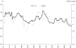
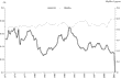
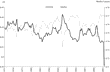
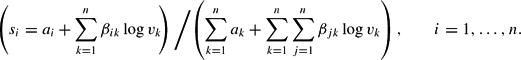
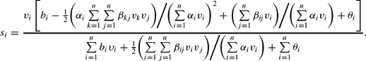
We report the income elasticities in panel A of Table 8, evaluated at the mean of the data, for the three subaggregates and for only the two demand systems that satisfy the theoretical regularity conditions at all data points—the generalized Leontief and the Minflex Laurent. All elasticities reported in this paper are based on the formulas used by Serletis and Shahmoradi (2005) and have been acquired using numerical differentiation. The income elasticities, ηAm, ηBm, and ηCm, are all positive, suggesting that assets A (M1), B (savings deposits), and C (time deposits) are all normal goods, which is consistent with economic theory. We believe there are actually good reasons to graph the income elasticities that we have estimated in Figures 1–3. Although not in contradiction to economic theory, there are small differences between the two models, as expected.


Income elasticity of A.

Income elasticity of B.

Income elasticity of C.
In panel B of Table 8 we show the own- and cross-price elasticities for the three assets. The own-price elasticities (ηii) are all negative (as predicted by the theory), with the absolute values of these elasticities being less than 1, which indicates that the demands for all three assets are inelastic. For the cross-price elasticities
, economic theory does not predict any signs, but we note that most of the off-diagonal terms are negative, indicating that the assets taken as a whole are gross complements. This is (qualitatively) consistent with the evidence reported by Serletis and Shahmoradi (2005) using the Fourier and AIM globally flexible functional forms.
In addition to the standard Marshallian price and income elasticities, which are directly relevant to many demand system applications, such as tax and welfare policy analyis, in Table 9 we show estimates of both the Allen and Morishima elasticities, evaluated at the means of the data. For panel A, we expect the three diagonal terms, representing the Allen own elasticities of substitution for the three assets, to be negative. This expectation is clearly achieved. However, because the Allen elasticity of substitution produces ambiguous results off diagonal, we will use the Morishima elasticity of substitution to investigate the substitutability/complementarity relation between assets. Based on the Morishima elasticities of substitution—the correct measures of substitution [see Blackorby and Russell (1989)]—as documented in panel B of Table 9, the assets are Morishima substitutes, with all Morishima elasticities of substitution being less than unity, irrespective of the model used.

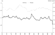
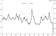
It is also interesting to present the graphs for the Morishima elasticities, in Figures 4–9. As already noted, the Morishima approach to the calculation of the elasticity of substitution provides a different estimate depending on which asset price is varied (of the two being considered). For example, Figure 4 shows the Morishima elasticity between assets A and B with the price of A changing, and Figure 5 shows the same elasticity with the price of B varying, in effect approaching from a different direction. As expected, there are no qualitative inconsistencies in the elasticity calculations and all the estimates are less than unity over the entire sample, showing mild substitutability (no matter what price is varied in the Morishima calculation).

Morishima elasticity of substitution between A and B with the price of A changing.

Morishima elasticity of substitution between A and B with the price of B changing.

Morishima elasticity of substitution between A and C with the price of A changing.

Morishima elasticity of substitution between A and C with the price of C changing.

Morishima elasticity of substitution between B and C with the price of B changing.

Morishima elasticity of substitution between B and C with the price of C changing.
SENSITIVITY OF RESULTS TO CURVATURE VIOLATIONS
We have argued that inferences based on the basic translog, AIDS, and (to a smaller extent) NQ reciprocal indirect utility function that violate theoretical regularity when the local curvature conditions are imposed will not significantly improve our understanding of real world money demand. In fact, we only presented results based on the generalized Leontief and Minflex Laurent models, for which all three theoretical regularity conditions (of positivity, monotonicity, and curvature) are satisfied at all data points when the local curvature conditions are imposed.
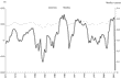
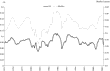
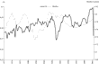
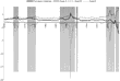
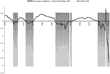
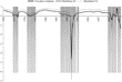
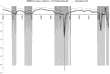
In this section we assess the effects of curvature violations on a model's ability to produce stable elasticity estimates, by presenting the basic translog income and Morishima elasticities of substitution in Figure 10 and Figures 11–13, respectively, along with information regarding the 50 data points at which curvature is violated (these are the vertically shaded points on the x axis). Clearly, there is considerable elasticity volatility in the data regions where curvature is not satisfied. In the literature, such elasticity volatility has been attributed to things other than model failure, such as, for example, in the case of the United States, to double-digit inflation after 1979, monetary decontrol, and the disinflation of the early 1980s.

Translog income elasticities.

Translog Morishima elasticities of substitution between A and B.

Translog Morishima elasticities of substitution between A and C.

Translog Morishima elasticities of substitution between B and C.
Here, we argue that it is the economic regularity violations that lead to the plots of wildly varying elasticities. In fact, the model produces such extremely unstable elasticity estimates that it is certainly useless for modeling the demand for money in the United States—similar elasticity graphs for the AIDS and the NQ reciprocal indirect utility function are available upon request.
REGULARITY EFFECTS OF SERIAL CORRELATION CORRECTION
We have used static models, implicitly assuming that the pattern of demand adjusts to a change in exogenous variables instantaneously. We paid no attention to the dynamic structure of the models used, although many recent studies report results with serially correlated residuals suggesting that the underlying models are dynamically misspecified. Autocorrelation in the disturbances has mostly been dealt with by assuming a first-order autoregressive process—see, for example, Ewis and Fisher (1984), Serletis and Robb (1986), Serletis (1987, 1988), Fisher and Fleissig (1994, 1997), Fleissig (1997), Fleissig and Swofford (1996, 1997), Fleissig and Serletis (2002), and Drake and Fleissig (2004).
In this section we investigate the effects on regularity of serial correlation corrections by allowing the possibility of a first-order autoregressive process in the error terms of equation (28), as follows,

where
is a matrix of unknown parameters and et is a nonautocorrelated vector disturbance term with constant covariance matrix. In this case, estimates of the parameters can be obtained by using a result developed by Berndt and Savin (1975). They showed that if one assumes no autocorrelation across equations (i.e., R is diagonal), the autocorrelation coefficients for each equation must be identical. Consequently, by writing equation (28) for period t−1, multiplying by R, and subtracting from (28), we can estimate stochastic budget share equations given by

We estimated the above equation for each of the generalized Leontief, translog, AIDS, Minflex Laurent, and NQ reciprocal indirect utility functions and observed that serial correlation correction increases the number of curvature violations and also leads to induced violations of monotonicity with most models, and in particular with the Minflex Laurent, AIDS, and translog—see Table 10.

It seems that the current practice of correcting for serial correlation without reporting the results of monotonicity checks (even when the curvature conditions are imposed) is not justified. Moreover, allowing for first-order serial correlation, as in equation (29), is almost the same as taking first differences of the data if the autocorrelation coefficient is close to unity. In that case, the equation errors become stationary, but there is no theory for the models in first differences.
We believe that in order to deal with dynamically misspecified models attention should be focused on the development of unrestricted dynamic formulations to accommodate short-run disequilibrium situations as, for example, in Serletis (1991) who builds on the Anderson and Blundell (1982) approach to dynamic specification in the spirit of error correction models. Alternatively, attention should be focused on the development of dynamic generalizations of the traditional static models by considering specific theories of dynamic adjustment.
CONCLUSION
We have argued that most published studies that use flexible functional forms do not reveal anything at all about violations of regularity, as also noted by Barnett (2002) and Barnett and Pasupathy (2003). Moreover, studies that equate curvature alone with regularity seem to ignore or minimize the importance of monotonicity. We argue that without satisfaction of all three theoretical regularity conditions (positivity, monotonicity, and curvature), the resulting inferences are worthless, because violations of regularity violate the maintained hypothesis and invalidate the duality theory that produces the estimated model. We believe that unless economic regularity is attained by luck, flexible functional forms should always be estimated subject to regularity.
We also revisited the demand for money in the United States in the context of five of the most popular locally flexible functional forms—the generalized Leontief, translog, almost ideal demand system, Minflex Laurent, and normalized quadratic reciprocal indirect utility function. In doing so, we treated the curvature property as a maintained hypothesis, using methods recently suggested by Ryan and Wales (1998) and Moschini (1999), and showed that (with our data set) the imposition of local curvature does not always ensure theoretical regularity, because of curvature violations at other points within the region of the data. We believe that this is a typical result in the literature that uses locally flexible functional forms and alert researchers to the kinds of problems that arise when all three theoretical regularity conditions are not satisfied; see also Barnett (2002) and Barnett and Pasupathy (2003).
Our results with the generalized Leontief and Minflex Laurent models that satisfy full regularity have implications for the formulation of monetary policy. They concur with the evidence presented by Serletis and Shahmoradi (2005), who use the globally flexible Fourier and AIM functional forms and impose global curvature, using methods suggested by Gallant and Golub (1984). The evidence indicates that the elasticities of substitution among the monetary assets (in the popular M2 aggregate) are consistently and believably below unity, suggesting that the simple sum approach to monetary aggregation is invalid, consistent with a large body of recent literature, both theoretical and empirical, that makes the same point. As we also argued in Serletis and Shahmoradi (2005), the Divisia method of aggregation solves this problem.
We have estimated money demand functions from aggregate time series data and highlighted the challenge inherent with achieving economic regularity and the need for economic theory to inform econometric research. Incorporating restrictions from economic theory seems to be gaining popularity, as there are also numerous recent papers that estimate stochastic dynamic general equilibrium models using economic restrictions; see, for example, Aliprantis et al. (2007). With the focus on economic theory, however, we have ignored econometric regularity. In particular, we have ignored unit root and cointegration issues, because the combination of nonstationary data and nonlinear estimation in large models such as the ones in this paper is an extremely difficult problem. In this regard, it should be noted, however, that the optimization methods suggested by Gallant and Golub (1984), and recently employed by Serletis and Shahmoradi (2005), are not subject to the substantive criticisms relating to econometric regularity.
Finally, it should be noted that an alternative approach to demand analysis is nonparametric, in the sense that it requires no specification of the form of the demand functions. This approach, originated by Varian (1982, 1983), has been used in numerous recent papers, such as, for example, Fleissig et al. (2000), Swofford and Whitney (1987, 1988, 1994), Fleissig and Whitney (2003, 2005), de Peretti (2005), Jones and de Peretti (2005), and Jones et al. (2005). It deals with the raw data itself and (using techniques of finite mathematics) typically addresses the issue of whether observed behavior is consistent with the preference maximization model. However, there are also advantages and disadvantages of this approach to demand analysis. As Fleissig et al. (2000, p. 329) put it,
the main advantage is that the tests are non-parametric; one need not specify the form of the utility function. Also, tests can handle a large number of goods. The main disadvantage is that the tests are non-stochastic. Violations are all or nothing; either there is a utility function that rationalizes the data or there is not.
This paper builds on material from Asghar Shahmoradi's Ph.D. dissertation at the University of Calgary. We would like to thank two referees of the journal for comments that greatly improved the paper and the members of Asghar Shahmoradi's Ph.D. dissertation committee: Frank Atkins, John Boyce, Herb Emery, Zuzana Janko, Gordon Sick, and James Swofford. Serletis gratefully acknowledges financial support from the Social Sciences and Humanities Research Council of Canada (SSHRCC).