


INTRODUCTION
Predictive models can have multiple applications, such as defining the most suitable areas for species reintroduction or protection, and understanding which environmental variables most accurately explain species distribution (Fielding & Haworth Reference Fielding and Haworth1995). When investigated at landscape, local or site spatial scales, then considering land-cover variables in modelling is recommended (Pearson & Dawson Reference Pearson and Dawson2003); at broader spatial scales, land cover can help to improve the explanatory power of bioclimatic models (Thuiller et al. Reference Thuiller, Araújo and Lavorel2004). Land-cover data may be a good substitute for genetically-based measures of determining population isolation in the context of conservation planning (Greenwald et al. Reference Greenwald, Gibbs and Waite2009a). Land-classification variables are used in different ways: some authors determine Euclidean distances to different classes (Alzaga et al. Reference Alzaga, Tizzani, Acevedo, Ruiz-Fons, Vicente and Gortázar2009); some calculate the surface area of each class (Herrmann et al. Reference Herrmann, Babbitt and Baber2005; Oja et al. Reference Oja, Alamets and Pärnamets2005; Egea-Serrano et al. Reference Egea-Serrano, Oliva-Paterna and Torralva2006; Acevedo et al. Reference Acevedo, Cassinello and Gortázar2007, Reference Acevedo, Farfán, Márquez, Delibes-Mateos, Real and Vargas2011; Delibes-Mateos et al. Reference Delibes-Mateos, Farfán, Olivero, Márquez and Vargas2009, Reference Delibes-Mateos, Farfán, Olivero and Vargas2010; Greenwald et al. Reference Greenwald, Gibbs and Waite2009a, Reference Greenwald, Purrenhage and Savageb); or combine both criteria (Hirzel et al. Reference Hirzel, Hausser, Chessel and Perrin2002; Seoane et al. Reference Seoane, Bustamante and Díaz-Delgado2004; Acevedo & Cassinello Reference Acevedo and Cassinello2009; Baasch et al. Reference Baasch, Fischer, Hygnstrom, VerCauteren, Tyre, Millspaugh, Merchant and Volesky2010); and yet others quantify every land class as 1 (present) or 0 (absent) (Guerry & Hunter Reference Guerry and Hunter2002; Svenning et al. Reference Svenning, Baktoft and Balslev2009). An alternative way of dealing with land classes in distribution modelling is to use them as categorical variables (Phillips et al. Reference Phillips, Anderson and Schapire2006; Yost et al. Reference Yost, Petersen, Gregg and Miller2008). However, each one of the formats involves different information on the relationship between species and landscape. The presence/absence of a class could provide information on whether a habitat is needed or avoided by a species within its territory (for example a species could need a water surface in its habitat), while the surface area of a land-cover class might suggest that a species is needing a relatively high or low cover area of a certain habitat (for example a species could need water to cover a high proportion of its habitat surface). In addition, the minimum distance to a land class in a model may suggest the need for a land-class to be accessible for a species (for example a species could simply need the presence of a water surface nearby).
The purpose of this study was to evaluate whether using different land classification approaches when constructing favourability models for Salamandra salamandra longirostris could influence the explanatory power of the models. Such comparison has not been made before. Salamander distribution modelling has been recurrently based on land-cover surfaces (see Herrmann et al. Reference Herrmann, Babbitt and Baber2005; Egea-Serrano et al. Reference Egea-Serrano, Oliva-Paterna and Torralva2006; Price et al. Reference Price, Dorcas, Gallant, Klaver and Willson2006; Greenwald et al. Reference Greenwald, Gibbs and Waite2009a, Reference Greenwald, Purrenhage and Savageb), and models combining land-cover variable types (though not for salamander) usually select a priori which type of variable is applied to every land-cover class (for example see Hirzel et al. Reference Hirzel, Hausser, Chessel and Perrin2002; Baasch et al. Reference Baasch, Fischer, Hygnstrom, VerCauteren, Tyre, Millspaugh, Merchant and Volesky2010). S. s. longirostris is endemic to the southern Iberian Peninsula, where major losses in environments suitable for amphibians have been predicted due to climate warming (Araújo et al. Reference Araújo, Thuiller and Pearson2006) and observed due to development, agriculture, reduced-habitat and other factors (Pleguezuelos et al. Reference Pleguezuelos, Márquez and Lizana2004; Stuart et al. Reference Stuart, Chanson, Cox, Young, Rodrigues, Fischman and Waller2004; Cruz et al. Reference Cruz, Rebelo and Crespo2006). Amphibians are especially vulnerable to habitat loss and fragmentation because they need relatively intact aquatic and terrestrial habitats (Cushman Reference Cushman2006) that maintain a level of homogeneity important for this species survival. The main danger to S. salamandra in Spain is the loss (either by aridification or by habitat destruction) of water points used for reproduction (Pleguezuelos et al. Reference Pleguezuelos, Márquez and Lizana2004). Such a degree of dependence on land cover may make a distribution model for S. salamandra sensitive to the way variables describing landscape are integrated in the model formulation.
METHODS
Study area and distribution data
The Iberian Peninsula is the most south-western territory in Europe (see Fig. 1a). Its varied orography and geographic position, lying between two continents (Europe and Africa) and between two water masses (Atlantic Ocean and Mediterranean Sea), determine a bioclimatically heterogeneous area (López Fernández et al. Reference López Fernández, Piñas and López2008). The study area is located in the southernmost part of the Iberian Peninsula, including all small Andalusian river basins south of the Guadalquivir River. These basins flow into the Mediterranean Sea or the Atlantic Ocean, and include the strongest precipitation gradient in Iberia, given that the Serranía de Ronda (between Cadiz and Malaga, in the west) is the rainiest region in the Iberian Peninsula, whereas Almeria province (in the east) is the one of the driest regions in Europe.

Figure 1 Study area and distribution data. (a) Geographical context. Mountains, main towns and the Guadalquivir River are shown as geographic references. (b) Sites (1-km2 squares) with presences, absences and pseudo-absences of Salamandra salamandra longirostris according to Tejedo et al. (Reference Tejedo, Reques, Gasent, González, Morales, García, González, Donaire, Sánchez and Marangoni2003) (see main text for explanation of pseudo-absences); presences are shown in black, absences in grey and pseudo-absences in white. (c) Presences and absences in 10-km2 UTM squares according to Pleguezuelos et al. (Reference Pleguezuelos, Márquez and Lizana2004).
Nine Salamandra salamandra subspecies live in the Iberian Peninsula. We studied the southernmost subspecies, S. s. longirostris (Los Barrios fire salamander), which is catalogued as vulnerable to extinction (VU) according to the International Union for the Conservation of Nature (IUCN; Pleguezuelos et al. Reference Pleguezuelos, Márquez and Lizana2004). Recent studies have classified S. s. longirostris as being sufficiently different to be considered a separate species (García-París et al. Reference García-París, Alcobendas and Alberch1998; Dubois & Raffaëli Reference Dubois and Raffaëli2009). Our study area involves 98.9% of the 10-km2 squares in which such endemic subspecies occurs (Pleguezuelos et al. Reference Pleguezuelos, Márquez and Lizana2004). S. s. longirostris is at risk because of the loss of aquatic habitats due to habitat destruction (Pleguezuelos et al. Reference Pleguezuelos, Márquez and Lizana2004). The distribution data of S. s. longirostris in 1-km2 grid squares was obtained using a database created by Tejedo et al. (Reference Tejedo, Reques, Gasent, González, Morales, García, González, Donaire, Sánchez and Marangoni2003); records were collected during surveys performed between 1980 and 2003 (with 80% having taken place after 1993) in the whole Andalusia region, surveying sites in the areas considered as potentially suitable for this species. Within our study area, S. s. longirostris was present in 388 of the sampled squares (that is all squares in which there was at least one amphibian species, according to the database) and absent from 330 (see Fig. 1b). Our study area involves 99.2% of the S. s. longirostris presences recorded by Tejedo et al. (Reference Tejedo, Reques, Gasent, González, Morales, García, González, Donaire, Sánchez and Marangoni2003). The surveying effort in some areas of Andalusia, including the most easterly part of our study area, was low because of the scarcity of optimum habitats for amphibians (Tejedo et al. Reference Tejedo, Reques, Gasent, González, Morales, García, González, Donaire, Sánchez and Marangoni2003). For modelling purposes, we generated a set of 80 pseudo-absences by selecting random points in this area using Hawth's tools and ESRI ArcMap 9.2 software. The complete absence of S. salamandra from this zone was confirmed by Pleguezuelos et al. (Reference Pleguezuelos, Márquez and Lizana2004).
Predictor variables
To determine the variables that best explain the distribution of S. s. longirostris, we compared species’ presences and absences (or pseudo-absences) to the distribution of 42 predictor variables associated with spatial situation (longitude and latitude), topography, climate and human activity, and to 28 land-cover classes extracted from the land-cover maps of Andalusia for 2003 according to Junta de Andalucía (2009) (see Table 1). These land classes were used to build three sets of predictor variables in all 1-km2 squares within the study area: presence-absence of every class; surface area covered by every class; and minimum Euclidean distance to every class. These types of variables were preferred to categorical variables because they allow every 1-km square to be associated with more than one land-cover class. Land-cover classes, initially in polygon shape-file format, were processed using the ESRI ArcMap 9.2 software. Polygons were converted to a 100 × 100-m resolution raster, and Euclidean distances to each polygon class were then computed using the ‘distance’ spatial-analyst tool. Finally, values of every presence, surface and distance variable in 1-km2 squares were extracted using the ‘zonal statistics as table’ spatial-analyst tool.
Table 1 Variables used to model the determinants of the distribution of Salamandra salamandra longirostris. Sources: 1Instituto Geográfico Nacional (1999); 2US Geological Survey (1996); 3Shuttle Radar Topography Mission (SRTM; Farr & Kobrick Reference Farr and Kobrick2000); 4Font (Reference Font1983); 5Instituto Geológico y Minero de España (1979); 6Font (Reference Font2000); 7Montero de Burgos and González-Rebollar (Reference Montero de Burgos and González-Rebollar1974); 8Junta de Andalucía (2009); 9Oak Ridge National Laboratory (2001).

Model building
The dependent variable used to build the models was the presence/absence of S. s. longirostris with n = 798 1-km2 grid squares; the species was present in 48.6% of the squares and absent or pseudo-absent in 51.4%.
We constructed the models using forward-backward stepwise logistic regression of the presence/absence (or pseudo-absence) data for all predictor variables. We built four different models. Every spatial, orographic, climatic and human variable (Table 1) was considered in all models, but a different set of land-cover variables was also proposed to the variable selection procedure in each model: (1) presence-absence of every land-cover class; (2) surface area covered by every class; (3) minimum Euclidean distance to every class; and (4) these three variable sets together. Finally, we applied the favourability function (Real et al. Reference Real, Barbosa and Vargas2006), which reflects the degree (between 0 and 1) to which the probability values obtained in each model differ from that expected according to the species’ prevalence (null model), being 0.5 the favourability value suggesting no difference between both probability values. Thus, favourability F for the presence of S. s. longirostris in each square was obtained by using the formula:
 \begin{equation}
F = [p/(1 - p)]/[(n_1 /n_0 ) + (p/[1 - p])]\end{equation}
\begin{equation}
F = [p/(1 - p)]/[(n_1 /n_0 ) + (p/[1 - p])]\end{equation}
To minimize type I errors due to the number of variables used in the analyses, we controlled the false discovery rate (FDR), that is, we avoided the false rejecting of the null hypothesis, which predicts that the distribution of S. s. longirostris cannot be modelled with the variable set (Table 1). The procedure outlined in Benjamini and Hochberg (Reference Benjamini and Hochberg1995) was used to control the FDR. This involves ordering the tested variables according to decreasing significance (increasing p-value), and only accepting variables up to the highest rank whose p -value is lower than i×q/V, where i is the rank of each variable in the ordered list, q is the critical FDR value, and V is the total number of tested variables. We took a critical value of q = 0.05, which implies that the selected variables were significant controlling for a FDR of q < 0.05.
The AIC of each model was compared to the AIC of the null model (we obtained this model from the 0-step of the stepwise procedure, before any variable has entered in the model). We also avoided excessive multicollinearity by checking the variable inflation factor (VIF) and pair-wise variable correlations (Appendix 1, Table S1, see supplementary material at Journals.cambridge.org/ENC). The VIF is considered acceptable up to 10, according to Montgomery and Peck (Reference Montgomery and Peck1992).
The relative weight of variables in each model was estimated using the Wald parameter. We also took into account the relative role of land-cover and other variables, and different groups of land-cover classes in the description of favourability. Thus, a variation partitioning procedure was performed to specify how much of the variation in favourability explained by the model was accounted for by the pure effect of each variable group (that is not affected by covariation with other variable groups in the model), and which proportion was clearly attributable to more than one group (shared effect) (Legendre Reference Legendre1993; Legendre & Legendre Reference Legendre and Legendre1998; for details of the procedure followed for variation partitioning, see Muñoz et al. Reference Muñoz, Real, Barbosa and Vargas2005).
Comparative assessment
Several indices were used to compare the performance of the four models. The area under the curve (AUC) of the receiver operating characteristic, which is independent of any favourability threshold (Hosmer & Lemeshow Reference Hosmer and Lemeshow2000), is a measure of the degree to which a species is restricted to part of the variation range of the modelled predictors, but is not a reliable measure of accuracy of the model's results (Lobo et al. Reference Lobo, Jiménez-Valverde and Real2008). However, a higher discrimination capacity could imply greater precision in describing the distribution of a species when two models of the same species in the same study area are compared. The Akaike information criterion (AIC) was employed as a measure of the degree of parsimony among models in a comparative set (Akaike Reference Akaike, Petrov and Csaki1973). A set of widely recognized measures of classification accuracy based on the 0.5-favourability threshold (as favourability is independent of prevalence, 0.5 is close to the favourability value at which both sensitivity and specificity are equal). These measures are as follows: correct classification rate (CCR), sensitivity, specificity, omission and commission errors, and Cohen's Kappa (which is described as the proportion of specific agreement; Fielding & Bell Reference Fielding and Bell1997). Each model's capacity to provide descriptions or inferences, that is, the per cent of presences in areas described as favourable, and of absences in areas described as unfavourable by the model, was assessed. To this end, squares whose favourability value was 0.8 or higher were considered favourable, whereas those with values equal to 0.2 or lower were considered unfavourable. This is equivalent to defining a prediction with odds higher than 4:1 as favourable, and lower than 1:4 as unfavourable (Rojas et al. Reference Rojas, Cotilla, Real and Palomo2001; Muñoz & Real Reference Muñoz and Real2006). Significant differences between models were assessed using the arcsine test of equality of percentages (Sokal & Rohlf Reference Sokal and Rohlf1979, p. 663). Each model's capacity to describe or infer was also evaluated by comparing how high the favourability values were, according to each model, in squares where presences have been observed, and how low these values were in squares from which the species was absent. The Wilcoxon test was used for these comparisons.
Each model's predictive capacity was defined in the same way as each model's descriptive capacity, but taking into account presences and absences obtained from an independent (not used for the model training) database (Fig. 1b). The data source was the Atlas and Red Book of Amphibians and Reptiles of Spain (Pleguezuelos et al. Reference Pleguezuelos, Márquez and Lizana2004), where presence/absence data are recorded in 10-km2 UTM (Universal Transverse Mercator) squares. The following steps were used to test each model's predictive capacity: (1) we projected the favourability values predicted by the model to each of the 21 880 1-km2 squares of the study area; (2) every 10-km2 UTM square was given the maximum favourability value observed in the 1-km2 squares located inside them; (3) using these 10-km2 resolution favourability values, and the information on presences/absences taken from the Atlas (Fig. 1b), we followed the same procedure used when evaluating each model's descriptive capacity.
RESULTS
The models
Using the four models (hereafter ‘Pres-Model’ for model using the presence or absence of every land-cover class, ‘Surf-Model’ for that using the surface area covered by every class, ‘Dist-Model’ for that using the minimum Euclidean distance to every class, and ‘All-Model’ for that combining all three variable sets) when favourability values were projected to every 1-km2 square in the study area, between 9.52% and 10.72% of the study area was classified as favourable and between 56.94% and 59.43% was classified as unfavourable for S. s. longirostris (Fig. 2). Regardless of the model, there is a central core of favourability in the western half of the study area. This nucleus corresponds to the main population of the Iberian endemic subspecies.
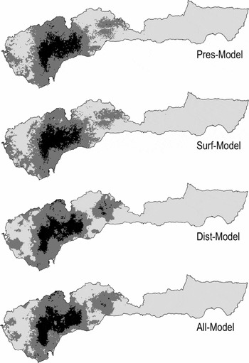
Figure 2 Models of Salamandra salamandra longirostris using the presence or absence of every land-cover class (Pres-Model), the surface area covered by every class (Surf-Model), the minimum Euclidean distance to every class (Dist-Model), and the three variable sets together (All-Model). Favourability values have been projected to every 1-km2 square throughout the study area. Favourable areas are shown in black (favourability value ≥ 0.8), unfavourable areas are in light grey (favourability value ≤ 0.2), and those with intermediate favourability are in dark grey (0.2 < favourability value < 0.8).
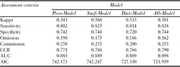
The AIC of the four models was always lower than 750 (Table 2, which was considerably lower than the null model AIC (1102.31). Conversely, multicollinearity seemed to be acceptable in all cases: no variable whose correlation was higher than 0.70 were included in the same model (Appendix 1, Table S2, see supplementary material at Journals.cambridge.org/ENC), and the inflation factor was never higher than 5.5 (Appendix 1, Table S1, see supplementary material).
Table 2 Comparative assessment of four models of the distribution of Salamandra salamandra longirostris according to classification, discrimination and parsimony criteria. CCR = correct classification rate; AUC = area under the ROC (receiving operating characteristic) curve; AIC = Akaike information criterion (for model names see Fig. 2).
The four models included land-cover variables, spatial situation, human activity, climate and topography (Table 3). In terms of non-land-cover variables, there were strong similarities among the four models: they shared all the climatic, topographic, spatial and human variables of importance according to their relative weight (see Wald parameter in Table 3), though the Pres- and Surf-Models also included variables associated with the number of days with precipitation (either rainfall, snow or storms; see Table 3). In both Pres- and Surf-Models, more than 95% of the explained variation in favourability was accounted for purely by non-land-cover variables; in both Dist- and All-Models this percentage was only around 50%, although the explained variation in favourability accounted for by both the pure effect of non-land-cover variables and the intersection between land-cover and non-land-cover variables was more than 90% (Fig. 3a).
Table 3 Predictor variables included in each favourability model (for abbreviations see Table 1). Signs in brackets show the positive or negative relationship between favourability and the variables in the models. The Wald parameter indicates the relative weight of every variable in the model (for model names see Fig. 2).


Figure 3 Variation partitioning diagrams to specify: (a) how much of the variation in favourability for Salamandra salamandra longirostris explained by the models was accounted for purely by land-cover and by non-land-cover variables, and which proportion was attributable to their shared effects (intersections), and (b) how much of the variation in favourability was accounted for purely by forested areas with oak, pastures, herbaceous crops and other land-cover classes, and their shared effects (intersections). Values shown are the percentages of variation explained (see Fig. 2 for explanation of model names).
In contrast, there were noticeable differences between the models according to which land-cover variables were included. In both Pres- and Surf-Models the pure effect of land cover only accounted for about 3% of the explained variation in favourability (and even less when the intersection between landscape and other factors was also considered), whereas in Dist-Model and in All-Model the pure effect of land cover accounted for 7% to 8%. This percentage, together with that of the intersection between land cover and other factors, ranged between 43% and 54% (see Fig. 3a). The four models provided different interpretations of which land-cover classes are important for S. s. longirostris: both Pres- and Dist-Models included oak woods (positively associated with favourability) and herbaceous crops (negatively associated with favourability), whereas Surf-Model included pastures and herbaceous crops (both negatively associated with favourability). Conversely, All-Model included a combination of the three types of land-cover variables (presence, surface area and Euclidean distance), and classes with oaks (short distance to them), pastures (low surface area) and herbaceous crops (poor presence and long distance to them) were accepted for entry in the model along the stepwise procedure (see Table 3 and Fig. 3b).
Comparative assessment
The model that combined three types of land-cover variables (All-Model) was the most parsimonious (lowest AIC), the best at classifying presences and absences (highest Kappa, sensitivity, specificity and CCR, and lowest omission and commission errors), and had the best discrimination capacity (highest AUC) (see Table 2). This was also the best model regarding the matches between presences and highly favourable areas when both the presences used to train the models and the presences of an independent data set were considered, although comparisons with the other models did not yield statistically significant differences in this regard (p > 0.05, see Table 4). Considering the data from the Atlas and Red Book of Amphibians and Reptiles of Spain (Pleguezuelos et al. Reference Pleguezuelos, Márquez and Lizana2004), All-Model obtained significantly fewer presences (p < 0.05) in highly unfavourable squares than Surf- and Dist-Models, but significantly more absences (p < 0.01) in highly favourable squares than Surf-Model (Table 4). On the other hand, All-Model obtained the significantly highest favourability values (p < 0.01) in the squares with presences used to train the models (Table 5); All-Model obtained significantly lower favourability values (p < 0.001) than both Pres- and Surf-Models (although higher than Dist-Model) in squares with absences, according to both the training and the Atlas data (Table 5).
Table 4 Percentage of presences and of absences in favourable (F ≥ 0.8) and unfavourable (F ≤ 0.2) areas. These percentages represent the model's capacity to describe the 1-km2 resolution distribution data of Salamandra salamandra longirostris in Tejedo et al. (Reference Tejedo, Reques, Gasent, González, Morales, García, González, Donaire, Sánchez and Marangoni2003), namely the data set used to train the models, and to predict the 10-km2 resolution distribution published in Pleguezuelos et al. (Reference Pleguezuelos, Márquez and Lizana2004), namely an independent data set. Brackets indicate the models with significant differences (arcsine test of equality of percentages: *p < 0.05; **p < 0.01). The models based on land-cover class presence, surface, distance and on a combination of these three variable types are named as ‘Pres’, ‘Surf’, ‘Dist’ and ‘All’, respectively.

Table 5 Probability in the between-model comparison of mean favourability values in squares where Salamandra salamandra longirostris is either present or absent from (Wilcoxon's test). In each comparison, mean favourability is higher in the model in rows. Significant difference when p < 0.05, ns = not significant (see Table 4 for explanation of model names).

Of the models that used only one land-cover variable type, Surf-Model was the best at classifying presences and absences and had the best discrimination capacity; Dist-Model was the most parsimonious (Table 2). The Surf-Model and the Dist-Model provided fewer matches between presences and highly favourable squares than the Pres-Model (Table 4). Conversely, all three models did not significantly differ in favourability values in squares where fire salamanders were present (p > 0.05, Table 5), although Dist-Model showed significantly lower favourability values than both Pres- and Surf-Models in squares with absences (according to both the training [p < 0.05] and the independent [p < 0.001] data sets; see Table 5).
DISCUSSION
Model comparison according to the variables selected
The models obtained describe areas favourable to S. s. longirostris as being humid mountainous lands in the east of the study area that are far from populated cities, most favourably among ecosystems associated with oak forests, but not with herbaceous ground (pastures and crops). This matches the known habitats of S. salamandra in southern Iberia (Miñano et al. Reference Miñano, Egea, Oliva-Paterna and Torralba2003; García-París et al. Reference García-París, Montori, Herrero, Ramos, Alba, Bellés, Gosálbez, Guerrera, Macpherson, Serrano and Templado2004). Our results are also compatible with those of Hermann et al. (Reference Herrmann, Babbitt and Baber2005) on amphibian distributions, in that landscape variables had less explanatory power than other factors, including climate (see Table 3 and Fig. 3a).
The four models are not identical to each other. In fact, only the two models that used Euclidean distances to land-cover classes, either alone (Dist-Model) or combined with other land-cover variable types (All-Model), identified a substantial role of land cover in explaining the areas favourable to S. s. longirostris; in contrast, the models that exclusively used either the presence (Pres-Model) or the surface area (Surf-Model) of land-cover classes gave most of the explanatory power to non-land-cover variables: climate, topography, spatial situation and distance to cities (see Fig. 3a). Variables related to water availability were selected as explanatory factors only when distances to land classes were excluded from the models. The highest correlations between mean annual days with precipitation and land cover involved distances to oak woods (r2 = –0.51) and distances to sparse scrub with oak (r2 = –0.42) (Appendix1, Table S2, see supplementary material at Journals.cambridge.org/ENC); similarly, correlations of these land-cover classes with mean annual storm days were among the highest values (r2 = –0.49 and r2 = –0.51, respectively). S. salamandra is preferably found in forests, but also in other land-cover types on condition that water points are available for reproduction (García-París et al. Reference García-París, Montori, Herrero, Ramos, Alba, Bellés, Gosálbez, Guerrera, Macpherson, Serrano and Templado2004). Thus, the presence of forests in surroundings grids could favour the presence of individuals found outside the forest itself. Water availability in the models where distances were excluded might indicate where conditions are most favourable to find forested habitats with oaks in the surroundings.
Once the distance to grids containing oak trees was accepted for entry in the models (both Dist-Model and All-Model), the intersection between the explanatory power of land-cover and non-land-cover variables increased above 34% (Fig. 3a), that is, more than 34% of the variation in favourability became indistinguishably explained by land-cover and by non-land-cover variables. This might be attributed to the fact that the humidity index, related to water availability and moderately correlated to oaks (Appendix1, Table S2, see supplementary material at Journals.cambridge.org/ENC), was included in all model with variables related to oak trees.
The description of the areas favourable for S. s. longirostris was supplied in its entirety only by the model that included land-cover variables expressed as presence, surface area and distance together. This model comprises all the qualitative information about favourable land-cover classes for Los Barrios fire salamanders and that was only partially included in each of the other three models.
Model comparison according to assessment parameters
The four favourability models for the distribution of S. s. longirostris obtained acceptable scores according to all the parameters considered to assess classification accuracy and discrimination capacity. Thus, Cohen's Kappa, which ranges from 0 to 1, was always higher than 0.5, being thus acceptable, according to Landis and Koch (Reference Landis and Koch1977). With values also ranging from 0 to 1, specificity was always higher than 0.7, sensitivity was higher than 0.8, the correct classification rate was higher than 0.75, and the omission and commission errors were lower than 0.2 and 0.3, respectively. Discrimination capacity (AUC, ranging from 0.5 to 1) was always higher than 0.880, and thus excellent, according to Hosmer and Lemeshow (Reference Hosmer and Lemeshow2000).
The differences between the values shown by the four models are slight (see Table 2). However, the model that combined the three types of land-cover variables (presence, surface area and distance) can certainly be considered the best. This is supported by the fact that this model repeatedly obtained the best values according to virtually all the parameters used in our assessment, including parsimony, classification accuracy, discrimination, and the capacity to describe the areas where fire salamanders occur as highly favourable and the areas where this species is absent as unfavourable.
In contrast, it is less obvious which of the models that used a single land-cover variable type was the best. In any case, the model that used the presence of land-cover classes alone was almost never the best compared to the models that used either the surface area or the distance to land classes. One reason for this might be that the information provided by the presence of a type of habitat is already provided by both the surface area of this habitat (where presence describes where the surface area is greater than zero) and the distance to it (presence means that the distance is zero). However, the latter provides additional information on the frequency and proximity of each land class that might contribute to the model's capacity to explain and describe a species’ distribution.
The role of land cover in the distribution of Salamandra salamandra longirostris: implications for conservation
We emphasize that our models describe the environmental needs of S. salamandra at a medium scale, but not necessarily at a micro scale. The ecological implications of our results regarding habitat needs should be interpreted as requirements for the most favourable occurrence of the species in 1-km2 squares, but not necessarily for the presence of individuals inside a given land-cover class. We are aware that salamanders require aquatic habitats for reproduction, which are located mainly in forests (Miñano et al. Reference Miñano, Egea, Oliva-Paterna and Torralba2003; Egea Serrano et al. Reference Egea-Serrano, Oliva-Paterna and Torralva2006) but also in pastures (García-París et al. Reference García-París, Montori, Herrero, Ramos, Alba, Bellés, Gosálbez, Guerrera, Macpherson, Serrano and Templado2004); however, our results do not provide information on reproductive needs in terms of the internal morphology and complexity of these habitats (for example, see Manenti et al. Reference Manenti, Ficetola and De Bernardi2009). This may be the reason why water surfaces did not appear in the models, with the exception of water canals, whose relative importance was very small (see Table 3 and Fig. 3b).
Three environments stand out in the models as important to S. s. longirostris in our study area: areas not far from oak (either forests or partially forested scrubland); areas either far from or lacking herbaceous crops; and areas where pastures do not predominate. Salvador and García-París (Reference Salvador and García-París2001) and García-París et al. (Reference García-París, Montori, Herrero, Ramos, Alba, Bellés, Gosálbez, Guerrera, Macpherson, Serrano and Templado2004) described landscapes favourable to S. salamandra in the Iberian Peninsula as those with moist forests with abundant dead plant substrate; this species needs highly developed vegetation cover that provides habitat diversity, shade, moderate temperature, moisture and organic matter (Hermann et al. Reference Herrmann, Babbitt and Baber2005). More specifically, oak forests are cited by Bousbouras and Ioannidis (Reference Bousbouras and Ioannidis1997) and Salvador and García-París (Reference Salvador and García-París2001) as frequent habitats for S. salamandra in Mediterranean landscapes. Non-forested areas are considered favourable for fire salamanders at high altitudes (Salvador & García-París Reference Salvador and García-París2001; García-París et al. Reference García-París, Montori, Herrero, Ramos, Alba, Bellés, Gosálbez, Guerrera, Macpherson, Serrano and Templado2004), in scrublands and grasslands (Salvador & García-París Reference Salvador and García-París2001), but not in deforested landscapes or monocultures (García-París et al. Reference García-París, Montori, Herrero, Ramos, Alba, Bellés, Gosálbez, Guerrera, Macpherson, Serrano and Templado2004). Our distribution models strongly indicate that the presence and the closeness of herbaceous agricultural areas, and the predominance of natural pastures, are unfavourable to the presence of S. s. longirostris. Rittenhouse et al. (Reference Rittenhouse and Semlitsch2006) and Greenwald et al. (Reference Greenwald, Purrenhage and Savage2009a, b) suggested that North American Ambystoma salamanders suffer from higher mortality and reduced mobility in open habitats (such as grasslands [Rittenhouse et al. 2006] and agricultural landscapes [Greenwald et al. Reference Greenwald, Gibbs and Waite2009a, Reference Greenwald, Gibbs and Waiteb]) than they do in forests. Both studies suggest that this is a consequence of population isolation due to habitat fragmentation. A relationship between local extinction and habitat fragmentation, mediated by interference with dispersers, was also described by Gibbs (Reference Gibbs1998) for woodland amphibians, including the salamander species Ambystoma maculatum. Our results appear to indicate that oak forest fragmentation in favour of pastures, and especially in favour of herbaceous crops, could be having a negative effect on the populations of the southernmost subspecies of S. salamandra in the Iberian Peninsula. Abundance decrease in populations as a consequence of human-caused forest loss are also reported for other salamander species, such as Eurycea cirrigera and Desmognathus fuscus stream salamanders in North Carolina (Price et al. Reference Price, Dorcas, Gallant, Klaver and Willson2006).
Throughout the study area, forests have been gradually replaced by herbaceous ecosystems during recent decades. The land-cover maps of Andalusia for 1956 and 2003 (Junta de Andalucía 2009) show that, in 47 years, the surface area of sparse scrub with oaks has suffered a 2.26% decrease, oak woods have decreased by 26.59%, whereas the surface areas of pastures, dry herbaceous crops and irrigated herbaceous crops have increased by 15.99%, 0.81% and 85.58%, respectively. Habitat changes in the study area may thus place S. s. longirostris populations in an unstable position from the point of view of conservation. Thus, habitat management aimed at avoiding forest fragmentation around the reproduction sites should be encouraged to conserve this subspecies. A deeper understanding of adult dispersion patterns, gained by closely monitoring S. s. longirostris, is also needed to guarantee maintaining its current populations.
CONCLUSIONS
Our aim was to evaluate whether the explanatory power of the models is altered when different approaches to the use of land-cover variables are considered in the construction of a favourability model for a case study based on the distribution of S. s. longirostris. Our results are based on a single example and so they cannot be unconditionally generalized. However, some useful information can be extracted from the analyses.
Among the models that were constructed using a single variable type for land cover, no model can be considered particularly better than the others according to the different approaches used for comparison. However our results do suggest that: (1) the model using the distance to land-cover classes alone gave a very important relative role to land cover in describing favourability, which may not necessarily be applicable to modelling other species in other study areas; and (2) the model using the presence of land-cover classes alone contributed little to what was explained by the other models. This is probably explained by the fact that the information provided by the presence of a given land-cover class is already provided by both the surface area occupied by that class and the distance to it. In qualitative terms, the three models focused on different (though not contradictory) sets of land-cover classes, and so every output may have driven a particular explanation of landscape use by S. s. longirostris. The best way to choose which type of land-cover variable should be used for modelling is probably to analyse the available knowledge on the biology of the species, and then to use the variable types that could serve to test a priori hypotheses about the relationships between species and habitat (see Greenwald et al. Reference Greenwald, Gibbs and Waite2009a).
In contrast, from both the quantitative and qualitative points of view, we consider that the model that jointly included various land-cover variable types robustly obtained the best performance, and so that this result could well be applicable to other areas and species beyond our case study. The main potential problem that could be caused by using several types of land-cover variables for every land class is the probability of increasing type I errors; too many variables entered in a model equation could lead to false results by pure chance (Benjamini & Hochberg Reference Benjamini and Hochberg1995; Hausdorf & Henning Reference Hausdorf and Henning2003). Procedures to control the false discovery rate (FDR; see for example Benjamini & Hochberg Reference Benjamini and Hochberg1995) can be used to avoid erroneously rejecting a true null hypothesis, as followed in the present study. The model that combined land-cover variable types not only obtained the best scores with almost every parameter computed for model assessment, but also provided the most complete information on the role of land cover to describe favourability. In its formulation, the model included the three environments whose importance had been partially suggested by the other models, and selected different types of land-cover variables for every environment. This provided improved insight into the ecological meaning of the model.
ACKNOWLEDGEMENTS
D. Romero was supported by a grant from the Ministerio de Educación: AP2007-03633. This study was partially supported by project CGL2009-11316 of the Ministerio de Ciencia e Innovación, and the European Commission under the HUNT project of the 7th Framework Programme for Research and Technological Development. We thank Dr Tejedo for the presence/absence data-set of Salamandra salamandra in Andalusia. We also thank S. Coxon for his help in the English revision of the manuscript.


