


1. Introduction
The formation of apparent sharp tips or points along deformable fluid interfaces has been of interest since it was reported more than four centuries ago by Gilbert (Reference Gilbert1958) that a sessile drop can be deformed into a conical profile by an electric field. Remarkably, such a response appears to also have been known to Lord Rayleigh who, in his seminal paper on the stability of a charged liquid drop (Rayleigh Reference Rayleigh1882), had somewhat unexpectedly but explicitly referred to the emission of fine jets from pointed protrusions on fluid interfaces. The general subject of the formation of apparent sharp tips or points at interfaces, however, began to be systematically and widely studied by mathematicians, scientists and engineers after a series of now-celebrated papers by Zeleny (Reference Zeleny1914, Reference Zeleny1917) on electrical discharges from the pointed tips of pendant drops. Within a short period following Zeleny's early work, the interest in the subject started growing after the publication of a number of papers during what can now be seen as the dawn of the field of electrohydrodynamics (EHD) (see below) and the publication of a landmark paper almost a century ago by Taylor (Reference Taylor1934) on emulsions. From a mathematical standpoint, a sharp point along an interface is the hallmark of a singularity as curvature, and therefore capillary pressure, often tend to infinity at sharp tips. Moreover, knowledge about the instability of such pointed interfaces is of tremendous importance in industrial applications in the absence as well as the presence of electric fields. If the interface is destabilized, entrainment of one phase into the other can occur. Thus, identifying the operating conditions under which interface instability followed by entrainment occurs is key in processes that do not ordinarily involve electric fields – such as emulsification by flow focusing and tip streaming (Anna, Bontoux & Stone Reference Anna, Bontoux and Stone2003; Suryo & Basaran Reference Suryo and Basaran2006; Barrero & Loscertales Reference Barrero and Loscertales2007; Castro-Hernández, Campo-Cortés & Gordillo Reference Castro-Hernández, Campo-Cortés and Gordillo2012; Gordillo, Sevilla & Campo-Cortés Reference Gordillo, Sevilla and Campo-Cortés2014; Evangelio, Campo-Cortés & Gordillo Reference Evangelio, Campo-Cortés and Gordillo2016) as well as selective withdrawal (Cohen & Nagel Reference Cohen and Nagel2002; Berkenbusch, Cohen & Zhang Reference Berkenbusch, Cohen and Zhang2008) where its occurrence is desirable, and air entrainment in coating flows (Blake & Ruschak Reference Blake and Ruschak1979; Scriven & Suszynski Reference Scriven and Suszynski1990; Simpkins & Kuck Reference Simpkins and Kuck2000; Kamal et al. Reference Kamal, Sprittles, Snoeijer and Eggers2019) where it is undesirable – but also in ones where electric fields are present (see below).
In the examples that have just been cited, interface deformation is driven by a flow that is typically extensional in nature and gives rise to hydrodynamic stresses which balance and grow with capillary stress. However, as has already been stated in the opening paragraph of this paper, electric fields acting on fluid interfaces also not only lead to the formation of shapes with singular curvature but the occurrence of such pointed interfaces resembling cones, cusps and wedges has an extremely rich history in EHD and the topic has remained at the forefront of research to this day. The goal of this work is to shed light on a recently discovered but currently poorly understood situation in EHD where an apparently singular interfacial profile can arise and, in some cases, be destabilized and result in interface rupture (Brosseau & Vlahovska Reference Brosseau and Vlahovska2017; Vlahovska Reference Vlahovska2019; Wagoner et al. Reference Wagoner, Vlahovska, Harris and Basaran2020; Marín Reference Marín2021).
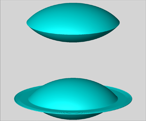
When a perfectly conducting drop surrounded by a perfectly insulating but less viscous exterior fluid is exposed to a strong electric field, the drop deforms in the direction of the applied field into a prolate profile and eventually takes on a spindle-like shape capped by conical ends. These sharp tips, which are now referred to as Taylor cones (Taylor Reference Taylor1964) (figure 1a), have been under continuous study since the pioneering experiments on electrified pendant drops by Zeleny (Reference Zeleny1914, Reference Zeleny1917), sessile soap bubbles by Wilson & Taylor (Reference Wilson and Taylor1925) and Macky (Reference Macky1930), and free drops by Nolan (Reference Nolan1924) and Macky (Reference Macky1931). What is remarkable is that a conical interface can exist in hydrostatic equilibrium solely under the balance between normal electric and capillary stresses and in the absence of hydrodynamic stresses if the drop is perfectly conducting (or perfectly insulating) and the exterior is perfectly insulating. If, however, the two phases are not perfect conductors/insulators, but the drop is a leaky dielectric (LD) (Taylor Reference Taylor1966; Smith & Melcher Reference Smith and Melcher1967; Melcher & Taylor Reference Melcher and Taylor1969; Saville Reference Saville1997) that is simply much more conducting than the exterior which is either perfectly insulating (e.g. a gas) or another LD fluid, electric tangential stresses enter the picture and disrupt the hydrostatic balance of forces. A thin jet of liquid is then emitted from the apex of the cone, giving rise to a phenomenon referred to as tip streaming (Collins et al. Reference Collins, Jones, Harris and Basaran2008, Reference Collins, Sambath, Harris and Basaran2013) or cone jetting (Fernández de La Mora Reference Fernández de La Mora2007; Marín et al. Reference Marín, Loscertales, Marquez and Barrero2007; Marín, Loscertales & Barrero Reference Marín, Loscertales and Barrero2008). If, however, the physical situation is inverted so that a weakly conducting and slightly viscous LD drop is immersed in a highly conducting and more viscous LD outer fluid, the drop deforms into an oblate shape and takes on a lens-like profile before eventually becoming unstable. From a macroscopic view, the equator of a lenticular drop superficially resembles a wedge prior to instability and such a drop disintegrates by equatorial streaming where a thin sheet of liquid is ejected from the drop's equator (Brosseau & Vlahovska Reference Brosseau and Vlahovska2017; Wagoner et al. Reference Wagoner, Vlahovska, Harris and Basaran2020).

Figure 1. (a) Left: a spherical drop subjected to an electric field – definition sketch. Top right: when subjected to a strong electric field, a perfectly conducting drop surrounded by a perfectly insulating exterior fluid is deformed into a prolate spindle shape with conical ends. Bottom: when subjected to a strong electric field, an LD drop surrounded by a more permittive, conducting and viscous LD fluid, however, is deformed into an oblate lenticular shape with a wedge-like equator. (b) When oriented about their apexes and overlaid by appropriately shifting the  $r$-axis in one case and the
  $z$-axis in the other, the conical (red line, Taylor cone) and wedge-like (black line, lens) geometries of the drops shown in panel (a) have similar cross-sections that appear to overlap locally. Here,
  $z_{tip}$ and
  $r_{eq}$ denote the tip location in the axial direction of the Taylor cone and the equatorial radius of the lens. All drop shapes shown have been obtained from simulations. Values of the parameters used in these simulations can be found in Appendix A.
We compare side-by-side in figure 1(b) the cross-sections of the spindle and lens-shaped droplets: when viewed again from a macroscopic perspective, the profiles of the two drops are remarkably similar near their tips – the two poles in the former case and the equator in the latter one (Appendix A). While the electrohydrostatic shapes and stability of highly deformed prolate electrified drops (Miksis Reference Miksis1981; Basaran & Scriven Reference Basaran and Scriven1982; Joffre et al. Reference Joffre, Prunet-Foch, Berthomme and Cloupeau1982; Basaran & Scriven Reference Basaran and Scriven1990; Basaran & Wohlhuter Reference Basaran and Wohlhuter1992; Wohlhuter & Basaran Reference Wohlhuter and Basaran1992; Ramos & Castellanos Reference Ramos and Castellanos1994b) and the physics that give rise to Taylor cones and their instability (Taylor Reference Taylor1964; Li, Halsey & Lobkovsky Reference Li, Halsey and Lobkovsky1994; Ramos & Castellanos Reference Ramos and Castellanos1994a; Burton & Taborek Reference Burton and Taborek2011) have been extensively investigated, similar studies for lens-shaped droplets which, however, involve flows driven by electric shear stresses, have been lacking.
It is noteworthy that lens-shaped drops have become of interest fairly recently. Indeed, the instability of lenticular drops is one of several types of instabilities that are exhibited by oblate drops under the influence of an applied electric field. The oblate instabilities of interest arise in situations in which the exterior fluid has a greater permittivity and is of relatively even greater conductivity than the drop. Such situations have been experimentally studied by Brosseau & Vlahovska (Reference Brosseau and Vlahovska2017) who fixed the ratio of the inner to the outer permittivity  $\kappa$ at 0.6 and varied both the ratio of conductivities and that of viscosities by several orders of magnitude. In their experiments, drops that are spherical in the absence of electric field deform into oblate shapes at low field strengths. When the ratio of the conductivity of the inner fluid to that of the outer fluid
  $\chi$ is greater than approximately 0.01, oblate drops undergo Quincke rotation when the field strength becomes sufficiently high. The response of oblate drops that are immersed in fluids of much larger conductivites depends on the ratio of their viscosities. When the ratio of the outer to the inner viscosity
  $\lambda$ is small, oblate drops take on dimpled or discocyte-shaped profiles and succumb to the dimpling instability where the drops break to form a torus. When
  $\lambda$, however, is large, the drops take on lenticular profiles and eject thin sheets from their equators. The steady-state shapes and stability of both dimpled and lenticular drops have been studied computationally by Wagoner et al. (Reference Wagoner, Vlahovska, Harris and Basaran2020). These authors have paid particular attention to situations at extreme values of the viscosity ratio, viz.
  $\lambda \ll 1$ and
  $\lambda \gg 1$. An overview of the subject along with recommendations for future studies can be found in the review by Vlahovska (Reference Vlahovska2019) and in a very accessible article by Marín (Reference Marín2021).
In this paper, we investigate by a combination of steady state, as well as transient simulations and theory, the apparently singular tips that are formed on the surfaces of lenticular drops, and also the conditions that are necessary for and the onset of equatorial streaming upon the destabilization of such drops. We show theoretically by carrying out a local analysis that the equatorial profile of a lenticular drop can be a wedge only if an approximate form of the surface charge transport equation known as the continuity of the normal current condition is employed in lieu of the full charge transport equation. Moreover, we demonstrate computationally that such wedge-shaped drops do not become unstable and therefore cannot emit equatorial sheets. We then show by transient simulations how equatorial streaming can occur when charge transport along the interface is analysed without approximation. We note that while the steady and dynamic states of LD drops that exhibit both prolate and oblate deformations have been widely studied in the literature for fifty years (Feng & Scott Reference Feng and Scott1996; Bentenitis & Krause Reference Bentenitis and Krause2005; Lac & Homsy Reference Lac and Homsy2007; Esmaeeli & Sharifi Reference Esmaeeli and Sharifi2011; Deshmukh & Thaokar Reference Deshmukh and Thaokar2013; Lanauze, Walker & Khair Reference Lanauze, Walker and Khair2013; Zabarankin Reference Zabarankin2013; Das & Saintillan Reference Das and Saintillan2017a), and the recent study by Wagoner et al. (Reference Wagoner, Vlahovska, Harris and Basaran2020) has reported results on the steady states and stability of lens-shaped drops, the destabilization of and equatorial streaming from lenticular drops have heretofore not been demonstrated computationally and hence remain inadequately understood (Marín Reference Marín2021).
The paper is organized as follows. Section 2 describes the mathematical formulation of the problem. A brief summary of the numerical method used in the simulations is then provided in § 3. Section 4 consists of three subsections. In the first, § 4.1, two sets of steady-state simulation results are presented and supplemented with a high-level overview of the physics of drop deformation caused by an applied electric field. In the second, § 4.2, the physics local to the equator of a lenticular drop is examined theoretically. In the last, § 4.3, conditions for the stability and instability of the equator as well as equatorial streaming from unstable drops are shown from dynamic simulations. Section 5 presents concluding remarks and a summary of possible directions for further study. The paper closes with two appendices. Appendix A presents a discussion on the values of the angles in the conical and wedge-like geometries of the drops depicted in figure 1(b). Appendix B provides a discussion of the range of values of the ratio of electrical relaxation time to the process/flow time, an issue that has received little attention in the literature.
2. Problem statement
The system (figure 1a) consists of two neutrally buoyant phases ( $i=1,2$;
  $i=1$, drop;
  $i=2$, exterior) each of which is an incompressible, Newtonian, LD (Melcher & Taylor Reference Melcher and Taylor1969; Saville Reference Saville1997) fluid of constant physical properties (viscosity
  $\mu _i$, permittivity
  $\epsilon _i$ and conductivity
  $\sigma _i$) undergoing Stokes flow. In the absence of an electric field,
  $\tilde {\boldsymbol {E}}_i = \boldsymbol {0}$, the drop is a sphere (radius
  $R$). It bears zero net charge. The interface separating the drop from the exterior has constant surface tension
  $\gamma$ as well as constant diffusivity for charge
  $\mathcal {D}_s$. We use a cylindrical coordinate system
  $(\tilde r, \varTheta , \tilde z)$ based at the centre of the undeformed drop and where these variables stand for the radial, angular and axial coordinates. The drop is subjected to an electric field
  $\boldsymbol {\tilde {E}_0} = \widetilde {E_0}\boldsymbol {e}_z$ of uniform strength
  $\tilde E_0$ far from its centre (
 $\boldsymbol {e}_z$ unit vector in
  $\tilde z$ direction). The problem is taken to be axisymmetric about
  $\varTheta$ or around the
  $\tilde z$-axis. It is non-dimensionalized using as characteristic scales
  $R$ for length,
  $t_c \equiv \mu _1 R/\gamma$ for time (
 $t_c$ visco-capillary time),
  $\gamma /R$ for hydrodynamic stress,
  $\tilde {E}_0$ for electric field,
  $\epsilon _2 \tilde {E}_0$ for surface charge density and
  $\epsilon _2 \tilde {E}_0^{2}$ for electric stress. Aside from the three dimensionless parameter ratios
  $\chi \equiv \sigma _1/\sigma _2$,
  $\kappa \equiv \epsilon _1/\epsilon _2$ and
  $\lambda \equiv \mu _2/\mu _1$, three other dimensionless groups arise: (1) electric Bond number
  $N_E \equiv \epsilon _2\tilde {E}^{2}_0 R / 2 \gamma$, which is the ratio of electric to capillary force; (2) dimensionless charge relaxation time in either phase
  $\alpha _i\equiv (\epsilon _i/\sigma _i)/t_c$ (
 $i=1$ or
  $2$), such that
  $\alpha _2/\alpha _1 = \chi /\kappa$; (3) Péclet number
  $Pe\equiv (R^{2}/\mathcal {D}_s)/t_c = \gamma R/\mu _1 \mathcal {D}_s$, which is the ratio of the time scale for charge diffusion on the surface
  $R^{2}/\mathcal {D}_s$ and the visco-capillary time
  $t_c$. In what follows, variables without tildes over them are the dimensionless counterparts of those with tildes over them, e.g.
  $\tilde r$ is dimensional but
  $r \equiv \tilde r/R$ is dimensionless.
In both domains ( $\varOmega _1$, which denotes the interior of the drop, and
  $\varOmega _2$, which denotes the region exterior to it), the electric field is irrotational and described by a potential (
 $\boldsymbol {E}_i = -\boldsymbol {\nabla }\varPhi _i$) which obeys the axisymmetric form of Laplace's equation
 \begin{equation} \nabla^{2} \varPhi_i = 0\quad \text{in}\ \varOmega _i. \end{equation}
The hydrodynamics in both phases is governed by the axisymmetric continuity and Stokes equations
 \begin{equation} \boldsymbol{\nabla}\boldsymbol{\cdot} \boldsymbol{v}_i = 0,\quad \boldsymbol{\nabla} \boldsymbol{\cdot} \boldsymbol{T}^{H}_i=\boldsymbol{0}\quad \text{in}\ \varOmega _i. \end{equation}
Here,  $\boldsymbol {v}_i$ is the velocity and
 \begin{equation} \boldsymbol{T}^{H}_i \equiv{-}p_i\boldsymbol{I} + (\mu_i/\mu_1)[(\boldsymbol{\nabla}\boldsymbol{v})_i + (\boldsymbol{\nabla}\boldsymbol{v})^{T}_i] \end{equation}
is the hydrodynamic stress where  $p_i$ is the pressure.
Along the drop surface  $S_f$, the flow and electric field in each phase are coupled through the traction condition which is the balance of momentum at the interface
 \begin{equation} \boldsymbol{n} \boldsymbol{\cdot} [\boldsymbol{T}^{H}_i + 2N_E\boldsymbol{T}^{E}_i]^{2}_1 = 2\mathcal{H} \boldsymbol{n}, \end{equation}
where
 \begin{equation} \boldsymbol{T}^{E}_i \equiv \frac{\epsilon_i}{\epsilon_2}\left(\boldsymbol{E}_i\boldsymbol{E}_i - \frac{1}{2}E^{2}_i\boldsymbol{I}\right) \end{equation}
is the electric (Maxwell) stress tensor (Melcher & Taylor Reference Melcher and Taylor1969),  $\boldsymbol {n}$ is the outward pointing unit normal to the drop's surface and
  $2\mathcal {H} \equiv \boldsymbol {\nabla }\boldsymbol {\cdot } \boldsymbol {n}$ is twice the mean curvature of the interface (Deen Reference Deen1998). The notation
  $[x]^{2}_1$ denotes the jump in
  $x$ in going from phase 1 to phase 2. Mass transfer across
  $S_f$ is prohibited by the kinematic boundary condition or the interfacial mass balance (Kistler & Scriven Reference Kistler and Scriven1983; Christodoulou & Scriven Reference Christodoulou and Scriven1992; Deen Reference Deen1998)
 \begin{equation} \boldsymbol{n} \boldsymbol{\cdot} \boldsymbol{v}_1 = \boldsymbol{n} \boldsymbol{\cdot} \boldsymbol{v}_2 = \boldsymbol{n} \boldsymbol{\cdot} \boldsymbol{v}_s, \end{equation}
where  $\boldsymbol {v}_s$ is the velocity of points along the interface. Additionally, along
  $S_f$, the tangential component of both the electric field and velocity field are continuous, viz.
  $\boldsymbol {t} \boldsymbol{\cdot} [\boldsymbol {E}_i]^{2}_1=0$ (Faraday's law) and
  $\boldsymbol {t} \boldsymbol{\cdot} [\boldsymbol {v}_i]^{2}_1=0$ (no slip) where
  $\boldsymbol {t}$ denotes the unit tangent to
  $S_f$ in the cross-sectional plane. The normal component of the electric displacement, however, suffers a discontinuity which is given by the surface charge density,
  $q \equiv \boldsymbol {n} \boldsymbol{\cdot} [(\epsilon _i/\epsilon _2)\boldsymbol {E}_i]^{2}_1$. In the LD model (Melcher & Taylor Reference Melcher and Taylor1969), bulk density of charge is zero but surface charge density on
  $S_f$ is governed by a transport equation as follows:
 \begin{equation} \alpha_2\left[q_t + \boldsymbol{\nabla}_s \boldsymbol{\cdot}(q\boldsymbol{v}) - Pe^{{-}1} \nabla^{2}_s q \right]= \left[\chi \boldsymbol{n} \boldsymbol{\cdot} \boldsymbol{E}_1 - \boldsymbol{n} \boldsymbol{\cdot} \boldsymbol{E}_2\right]\quad \text{on}\ S_f. \end{equation}
Here, subscript  $t$ denotes the partial derivative with respect to time
  $t$,
$t$,  $\boldsymbol {v}$ is the velocity and
  $\boldsymbol {E}_1$ and
  $\boldsymbol {E}_2$ are the electric fields at
  $S_f$, and
  $\boldsymbol {\nabla }_s$ is the surface gradient. In this equation, the terms on the left-hand side represent surface charge transport by convection and diffusion and the source-like terms on the right-hand side represent charge transport from each phase to
  $S_f$ by Ohmic conduction. In the limit that charge transport by diffusion and convection are negligible (Taylor Reference Taylor1966; Melcher & Taylor Reference Melcher and Taylor1969), this equation reduces to the continuity of the normal component of the electric current,
  $\boldsymbol {n} \boldsymbol{\cdot} [(\sigma _i/\sigma _2)\boldsymbol {E}_i]^{2}_1=0$. We note that this approximate form of the surface charge transport equation results from formally setting
  $\alpha _2 = 0$ in (2.7).
3. Simulations and numerical methods
Except when carrying out a local theoretical analysis, the governing equations are solved by numerical simulation using a transient but axisymmetric, finite-element-based algorithm over one quadrant of the  $rz$-plane (
 $r$,
$r$,  $z\geq 0$). The algorithm relies on the elliptic mesh generation method developed by Christodoulou & Scriven (Reference Christodoulou and Scriven1992), and which was later extended to drop dynamics problems with breakup by Notz & Basaran (Reference Notz and Basaran2004), for spatial discretization and for enabling capturing the evolution in time (or, as discussed below, with respect to a control parameter) of highly deformed interface shapes. The governing equations are solved subject to symmetry conditions along
  $r=0$ (axis of symmetry) and
  $z=0$ (plane of symmetry). Far from the drop's centre-of-mass, the electric potential is set to asymptotically approach that of a uniform field and the flow field is taken to be stress-free. While the formulation above is general, steady-state solutions can be obtained by: (i) setting
  $q_t=0$ in the surface charge transport equation (2.7); (ii) replacing the kinematic boundary condition by its steady state form
  $\boldsymbol {n} \boldsymbol{\cdot} \boldsymbol {v}_1 = \boldsymbol {n} \boldsymbol{\cdot} \boldsymbol {v}_2 = 0$ (for a steady flow,
  $\mathbf {n} \boldsymbol{\cdot} \mathbf {v}_s =0$); (iii) adding the capability to do continuation in a parameter using adaptive parameterization (Abbott Reference Abbott1978), track solution families (Feng & Basaran Reference Feng and Basaran1994) and automatically detect points where changes of stability occur (Brown & Scriven Reference Brown and Scriven1980; Ungar & Brown Reference Ungar and Brown1982; Yamaguchi, Chang & Brown Reference Yamaguchi, Chang and Brown1984). The steady-state version of the algorithm reduces to that used by Wagoner et al. (Reference Wagoner, Vlahovska, Harris and Basaran2020). Further details on the algorithm can be found in publications where similar versions and/or certain portions of the algorithm employed here are described and which have been used for solving equilibrium (Basaran & Scriven Reference Basaran and Scriven1990; Sambath & Basaran Reference Sambath and Basaran2014), steady state (Basaran & Scriven Reference Basaran and Scriven1988; Wagoner et al. Reference Wagoner, Vlahovska, Harris and Basaran2020) and transient (Collins et al. Reference Collins, Jones, Harris and Basaran2008, Reference Collins, Sambath, Harris and Basaran2013) problems in EHD. In all simulations,
  $Pe=10^{3}$ (Collins et al. Reference Collins, Jones, Harris and Basaran2008, Reference Collins, Sambath, Harris and Basaran2013). We note that all simulation results presented in the paper are insensitive to changes in
  $Pe$ provided that
  $Pe\gg 1$, as has already been demonstrated by Wagoner et al. (Reference Wagoner, Vlahovska, Harris and Basaran2020) in their study that involved computation of only steady-state solutions.
4. Results and discussion
4.1. Qualitative description of drop deformation and results of steady-state simulations
For systems in which the drop is a LD and the outer fluid is an insulator, a situation that is typically encountered in electrospray ionization spectroscopy (Fenn et al. Reference Fenn, Mann, Meng, Wong and Whitehouse1989; Fernández de La Mora Reference Fernández de La Mora2007) and electrically driven desalting of crude oil (Waterman Reference Waterman1965; Scott, DePaoli & Sisson Reference Scott, DePaoli and Sisson1994), or for systems in which both phases are LDs, which is common in operations involving electrospraying of one liquid into another in materials science and separations applications (Scott & Wham Reference Scott and Wham1988, Reference Scott and Wham1989; Harris, Scott & Byers Reference Harris, Scott and Byers1992; Ptasinski & Kerkhof Reference Ptasinski and Kerkhof1992), the applied electric field can cause drop deformation via two means. One is by the generation and action of electric normal stress at the interface separating the drop from the exterior fluid
 \begin{equation} [\boldsymbol{T}^{E}_{nn}]^{2}_1 \equiv \boldsymbol{n} \boldsymbol{\cdot} \left[\boldsymbol{T}^{E}_i\right]^{2}_1 \boldsymbol{\cdot} \boldsymbol{n} = \tfrac{1}{2} \left[E_{2,n}^{2} - \kappa E_{1,n}^{2} + E_t^{2} (\kappa -1)\right], \end{equation}
where  $E_{i,n} \equiv \boldsymbol {n} \boldsymbol{\cdot} \boldsymbol {E}_i$ and
  $E_t \equiv \boldsymbol {t} \boldsymbol{\cdot} \boldsymbol {E}_i$. The other is by the action of hydrodynamic normal stress at the interface separating the two fluids
 \begin{equation} \left[\boldsymbol{T}_{nn}^{H}\right]^{2}_1\equiv \boldsymbol{n} \boldsymbol{\cdot} \left[\boldsymbol{T}^{H}_i\right]^{2}_1 \boldsymbol{\cdot} \boldsymbol{n}, \end{equation}
which results from the flows induced by the electric tangential stress acting at the drop surface
 \begin{equation} \left[\boldsymbol{T}^{E}_{nt}\right]^{2}_1 \equiv \boldsymbol{n} \boldsymbol{\cdot} [\boldsymbol{T}^{E}_i]^{2}_1 \boldsymbol{\cdot} \boldsymbol{t} = \left(E_{2,n}-\kappa E_{1,n}\right)E_t \equiv q E_t. \end{equation}
 In the absence of charge convection and diffusion, the surface charge transport equation (2.7) reduces to  $\chi E_{1,n}=E_{2,n}$ and the electric stresses take on particularly simple and readily appreciable forms. In this limit, the electric normal stress (see (4.1)) becomes
 \begin{equation} [\boldsymbol{T}^{E}_{nn}]^{2}_1 = \frac{1}{2} \left[E_{1,n}^{2} (\chi^{2} - \kappa) + E_t^{2} (\kappa -1)\right] = \frac{1}{2} \left\{E_{1,n}^{2} \kappa^{2} \left [ \left ( \frac {\chi}{\kappa} \right )^{2} - \frac {1}{\kappa} \right ] + E_t^{2} (\kappa -1) \right\} \end{equation}
and the expression for the electric tangential stress (see (4.3)) reduces to
 \begin{equation} \left[\boldsymbol{T}^{E}_{nt}\right]^{2}_1 =E_{1,n} (\chi - \kappa) E_t = E_{1,n} \kappa \left ( \frac {\chi}{\kappa} - 1 \right )E_t \equiv q E_t . \end{equation}
While the nature of the stresses can now be examined in general both in the presence and the absence of charge convection and diffusion, we restrict the following discussion to a set of material properties that are known from experiments (Brosseau & Vlahovska Reference Brosseau and Vlahovska2017) to lead to lens-shaped drops and equatorial streaming. Thus, we focus on situations when the exterior fluid has a greater permittivity and is of relatively even greater conductivity than the drop,  $\chi /\kappa = ({\epsilon _2}/{\sigma _2})({\sigma _1}/{\epsilon _1})<1$ and
  $\kappa ={\epsilon _1}/{\epsilon _2}<1$. In the absence of charge convection and diffusion, it then follows from (4.4) that when
  $\chi /\kappa < 1$ and
  $\kappa < 1$, the electric normal stress
  $[\boldsymbol {T}^{E}_{nn}]^{2}_1 \le 0$ or is compressive (acts inward) everywhere on the surface of the drop regardless of its shape. The values of the electric tangential stress as well as the surface charge density in this limit are discussed below.
Some useful qualitative insights into how a LD drop would respond to an imposed uniform electric field can be gained by starting with an analysis of the electric stresses in the absence of charge convection and diffusion when the drop is spherical. In this limit, the electric field inside the spherical drop is uniform and given by  $\boldsymbol {E}_1=3\boldsymbol {e}_z(\chi +2)^{-1}$, where the unit vector
  $\boldsymbol {e}_z$ in the axial direction is related to the unit vectors in spherical coordinates
  $(\rho ,\phi ,\varTheta )$ as
 \begin{equation} \boldsymbol{e}_z = \cos \phi \boldsymbol{e}_{\rho} - \sin \phi \boldsymbol{e}_{\phi}. \end{equation}
Here,  $\rho$ is the radial coordinate in spherical coordinates or, equivalently, the distance measured from the centre of the drop,
  $0 \le \phi \le {\rm \pi}$ is the cone angle measured from the positive
  $z$-direction, and
  $0 \le \varTheta < 2{\rm \pi}$ is the angle measured about the axis of symmetry, and the unit normal and tangent vectors to the surface of the spherical drop are given by
  $\boldsymbol {n} = \boldsymbol {e}_{\rho }$ and
  $\boldsymbol {t} = \boldsymbol {e}_{\phi }$. Hence, the normal and tangential components of the electric field at the surface of the sphere are
 \begin{equation} E_{1,n} = \frac {3\cos \phi}{\chi + 2} \quad {\text{and}}\quad E_t ={-} \frac {3\sin \phi}{\chi + 2} . \end{equation}
In this situation,  $E_{1,n} \ge 0$ and
  $q \equiv E_{1,n}(\chi - \kappa ) \le 0$ on the top half of the drop and
  $E_{1,n} \le 0$ and
  $q \equiv E_{1,n}(\chi - \kappa ) \ge 0$ on the bottom half of the drop while
  $E_t \le 0$ over the entire surface. Thus, the electric tangential stress
  $[\boldsymbol {T}^{E}_{nt}]^{2}_1 = qE_t \ge 0$ on the top half of the drop and
  $[\boldsymbol {T}^{E}_{nt}]^{2}_1 = qE_t \le 0$ on the bottom half of the drop, and the flow along the free surface is from the drop's poles to its equator. When the surrounding fluid is also much more viscous than the drop (
 $\lambda \gg 1$), the hydrodynamic normal stresses accompanying the flow lead to an increase in equatorial curvature and a decrease in curvature at the poles, thereby inducing the spherical drop to undergo an oblate deformation (Wagoner et al. Reference Wagoner, Vlahovska, Harris and Basaran2020). Furthermore, in this situation, the electric normal stresses are compressive (act inward) along the surface of the originally spherical drop, as has already been discussed in the previous paragraphs. Indeed, the electric normal stresses at the poles of the sphere are given by
  $E_1^{2}(\chi ^{2} - \kappa )/2$ while that at the equator are given by
  $E_1^{2}(\kappa - 1)/2$. Thus, when
  $\chi \to 0$, which is a condition that favours equatorial streaming in experiments, the difference between the electric normal stress at the poles and that at the equator is given by
  $E_1^{2}(-2\kappa + 1)/2$. Therefore, as long as
  $\kappa \geq \frac {1}{2}$, the electric normal stress at the pole is more compressive than that at the equator, which also causes the equatorial curvature to increase and the curvature at the poles to decrease (Wagoner et al. Reference Wagoner, Vlahovska, Harris and Basaran2020). While the approach that has just been used to gain qualitative insights into the deformation of spherical drops can be replicated if the drops were spheroids (Lanauze, Walker & Khair Reference Lanauze, Walker and Khair2015), it is nevertheless reliant upon and hence limited by the assumption that both charge convection and diffusion are negligible. Therefore, we examine next the impact of charge convection and diffusion in two otherwise identical systems.
Figure 2(a) shows in a bifurcation diagram the variation of the steady-state deformation of the drop  $D\equiv (z|_{pole}-r|_{eq})/(z|_{pole}+r|_{eq})$ with electric Bond number
  $N_E$ for two systems. Here, the poles of the drop are located at
  $(r,z)=(0,\pm z|_{pole})$ and
  $r_{eq}$ stands for the equatorial radius of the drop. In both of these systems, the exterior fluid is more viscous (
 $\lambda = 25$), is more conducting (
 $\chi = 10^{-2}$) and has a higher permittivity or is more permittive (
 $\kappa = 0.5$) than the drop. The sole difference between these two systems is that the balance of normal currents (where
  $\alpha _2 = 0$) is imposed in one case and the full surface charge transport equation (with
  $\alpha _2=2$) is used in the other case. Figure 2(a) shows that when the strength of the applied electric field is weak (
 $N_{E}<0.5$) and consequently the deformation of the drop is small (
 $|D|<0.1$), drop deformation
  $D$ varies linearly with
  $N_E$ along each solution family and that there is negligible difference between the response of the system for which the balance of normal currents applies and the other for which the full charge transport equation is solved. Evidently, charge convection/diffusion plays a small role in determining the response of slightly deformed oblate shapes. As
  $N_E$ increases, however, the steady-state responses of the drops in the two cases begin to differ albeit while still sharing some common features. In both systems, at larger
  $N_E$, the variation of drop deformation with
  $N_E$ slows on the drop-scale (as measured by
  $D$) and the stresses at the equator grow rapidly (Wagoner et al. Reference Wagoner, Vlahovska, Harris and Basaran2020) with increasing electric Bond number and/or deformation. While the aforementioned features are common to both systems, whether charge diffusion and convection are allowed or not changes considerably the fates of the two solution families at large
  $N_E$. Although it is well known that accounting for charge convection reduces the deformation of oblate shapes compared with when it is neglected (Feng Reference Feng1999; Das & Saintillan Reference Das and Saintillan2017a,Reference Das and Saintillanb), the impact of these charge transport mechanisms on droplet stability has heretofore been unknown. Figure 2(b) shows clearly that a turning point, which signals a change of stability, is encountered along the shape family for which
  $\alpha _2=2$, no turning point arises along the shape family for which
  $\alpha _2 = 0$ or when the balance of normal currents is imposed. Figure 3 shows the variation of the reciprocal of twice the mean curvature at the equator,
  $(2\mathcal {H})|_{eq}^{-1}$, with electric Bond number
  $N_E$ along the steady-state solution families depicted in figure 2. In both cases, twice the mean curvature at the equator (its reciprocal) rises (falls) as
  $N_E$ increases, a point that is discussed further in the next paragraph. In order to gain further insights into the differences caused by charge convection and diffusion at large
  $N_E$ and which are shown in figures 2 and 3, we next examine the equatorial normal stresses along these two solution families.

Figure 2. Bifurcation diagram for steady-state solutions when the exterior fluid is more viscous ( $\lambda = 25$), conducting (
 $\chi = 10^{-2}$) and permittive (
 $\kappa = 0.5$) than the drop. (a) Variation of deformation
  $D$ with electric Bond number
  $N_E$ when the balance of normal currents is imposed (
 $\alpha _2 = 0$, red curve) and the full surface charge transport equation is solved (
 $\alpha _2=2$, grey curve). The open square in panel (a) highlights the region of the parameter space where the turning point is located when
  $\alpha _2 = 2$, i.e. when charge convection and diffusion are accounted for. (b) Zoomed-in view of the portion of the parameter space highlighted by the open square in panel (a). The turning point along the solution family of
  $\alpha _2=2$ is marked by an open circle.

Figure 3. Variation of the reciprocal of twice the mean curvature at the equator,  $(2\mathcal {H})|_{eq}^{-1}$, with electric Bond number
  $N_E$ along the steady-state solution families depicted in figure 2 (
 $\lambda = 25$,
  $\chi = 10^{-2}$ and
  $\kappa = 0.5$). The colour scheme is identical to that used in figure 2 such that red curves correspond to the system in which the balance of normal currents holds (
 $\alpha _2=0$), and grey curves correspond to the system when the full surface charge transport equation is solved (
 $\alpha _2=2$). (a) Here
  $(2\mathcal {H})|_{eq}^{-1}$ as a function of
  $N_E$. The open square in panel (a) highlights the region of the parameter space where the turning point is located when
  $\alpha _2 = 2$, i.e. when charge convection and diffusion are accounted for. (b) Zoomed-in view of the portion of the parameter space highlighted by the open square in panel (a). The turning point along the solution family of
  $\alpha _2=2$ is marked by an open circle.
Figure 4(a) shows the evolution of the equatorial normal stresses, viz. the hydrodynamic normal stress evaluated at the equator,  $[\boldsymbol {T}^{H}_{nn}]^{2}_1 |_{eq}$, and the absolute value of the electric normal stress at the equator,
  $2 N_{E} | [\boldsymbol {T}^{E}_{nn}]^{2}_1 |_{eq} |$, with the reciprocal of twice the mean curvature at the equator, viz.
  $(2\mathcal {H})|_{eq}^{-1}$, for the two shape families of figure 2. In the undeformed state or when the drop is spherical,
  $(2\mathcal {H})|_{eq}^{-1} = 1/2$. As the deformation of the drop increases,
  $(2\mathcal {H})|_{eq}^{-1}$ decreases. Given that the drop adopts a lenticular profile and that the radial location of the equator varies only slightly with electric Bond number for large
  $N_E$, the precipitous decrease in
  $(2\mathcal {H})|_{eq}^{-1}$ with
  $N_E$ shown in figure 3 captures well the precipitous decrease in the in-plane radius of curvature of the drop at the equator as
  $N_E$ increases. While figure 4(a) reveals that there are slight differences in the equatorial normal stresses between the system for which
  $\alpha _2=0$ and that for which
  $\alpha _2=2$ for small deformations (
 $(2\mathcal {H})|_{eq}^{-1}\approx 10^{-1}$), the differences between these two systems become stark as
  $(2\mathcal {H})|_{eq}^{-1}\to 0$. For the system with
  $\alpha _2=2$, the turning point occurs when
  $(2\mathcal {H})|_{eq}^{-1}\approx 10^{-3}$ and for the states near the turning point, the electric normal stress is an order of magnitude smaller than the capillary and hydrodynamic normal stresses. For the system with
  $\alpha _2=0$ and for which a turning point is not observed,
  $(2\mathcal {H})|_{eq}^{-1}$ is an order of magnitude smaller at large
  $N_E$ compared with the system with
  $\alpha _2 = 2$ and all normal stresses are of comparable orders of magnitude. In other words, no stress can be neglected as
  $N_E$ increases for the system in which the balance of normal currents is imposed. Given that instability is not observed in the case of
  $\alpha _2=0$ from simulations even when
  $(2\mathcal {H})|_{eq}^{-1}\approx 10^{-5}$, we next theoretically examine the limit
  $(2\mathcal {H})|_{eq}^{-1} \to 0$ for which the equator of the lenticular drop is wedge-like. Furthermore, we perform additional theoretical analyses to draw certain conclusions about the effect of charge convection and diffusion on the local behaviour of the various terms in the surface charge transport equation.

Figure 4. Equatorial normal stresses for the steady-state solutions depicted in figure 2. (a) Variation of the equatorial normal stresses with the reciprocal of twice the mean curvature at the equator,  $(2\mathcal {H})|_{eq}^{-1}$. The colour scheme is identical to that used in figure 2: red curves represent stresses when the balance normal currents holds (
 $\alpha _2=0$), and grey curves represent stresses when the full surface charge transport equation is solved (
 $\alpha _2=2$). Dash–dot–dotted curves represent the hydrodynamic normal stress,
  $[\boldsymbol {T}^{H}_{nn}]^{2}_1$, at the equator and solid curves represent the absolute value of the electric normal stress,
  $2N_{E} | [\boldsymbol {T}^{E}_{nn}]^{2}_1 |$, at that location. The horizontal arrow pointing from right to left, with
  $|D| \uparrow$ above it, indicates the direction in which the drop deformation
  $D$ increases. The open squares in panel (a) highlight the region of the parameter space where the turning point is located when
  $\alpha _2 = 2$. (b) Zoomed-in view of the portion of the parameter space highlighted by the open squares in panel (a). The turning point along the solution family of
  $\alpha _2=2$ is marked by open circles. While the horizontal (abscissa) axis is still
  $(2\mathcal {H})|_{eq}^{-1}$, the vertical axis label and the ordinate values on the right are those for
  $[\boldsymbol {T}^{H}_{nn}]^{2}_1$ at the equator and the corresponding quantities on the left are those for
  $2N_{E} | [\boldsymbol {T}^{E}_{nn}]^{2}_1 |$ at that location. Note that while the open circles indicate the values of the stresses and the reciprocal of twice the mean curvature at the turning point with respect to
  $N_E$, the curves showing the variation of stress with
  $(2\mathcal {H})|_{eq}^{-1}$ may not even exhibit turning because
  $(2\mathcal {H})|_{eq}^{-1}$ unlike
  $N_E$ (as in figure 2) is not the control parameter.
4.2. Local theoretical analysis in the neighbourhood of the equator
As can be seen from the simulation results shown in figure 1 and experimental images in figure 2 of Brosseau & Vlahovska (Reference Brosseau and Vlahovska2017), from the macroscale point of view the equator of the lenticular drop resembles a wedge. Hence, we will now carry out a local analysis to theoretically determine the electric field and stress distributions for a perfect wedge and compare these predictions with simulation results. In the analysis, we consider an infinite planar wedge of semiangle  $\beta$, and place the origin of a polar coordinate system (
 $\hat {r}$,
  $\theta$) at the apex of the wedge (figure 5a). The angle of the wedge at the equator of the lenticular drop is acute (
 $0 < \beta < {\rm \pi}/2$), and the drop (which is less conducting, viscous and permittive) occupies the portion of the region corresponding to
  $\theta > ({\rm \pi} -\beta )$ and the exterior surrounding fluid (more conducting, viscous and permitting) occupies the portion of the plane given by
  $\theta < ({\rm \pi} -\beta )$ (here, we only consider half the domain or the range
  $0 \le \theta \le {\rm \pi}$ because the profile of the wedge is symmetric about the midplane (
 $\theta =0, {\rm \pi}$)). For this wedge, we search for local solutions to Laplace's equation (2.1) that are antisymmetric about the midplane and are non-dominant over the electric potential corresponding to a uniform applied field far away. Solutions of this type are well known and/or easily obtained using separation of variables,
 \begin{equation} \left.\begin{gathered} \phi_2(\hat{r},\theta) = A_2 \hat{r}^{n}\sin\left(n\theta\right),\\ \phi_1(\hat{r},\theta) = A_1 \hat{r}^{n}\sin\left(n\left({\rm \pi}-\theta\right)\right), \end{gathered}\right\} \end{equation}
where  $A_2$ and
  $A_1$ are constants, and the index/exponent
  $n$ is real, positive and less than one. Determining the electric field (
 $\boldsymbol {E}_i = -\boldsymbol {\nabla }\varPhi _i$) from the interior and exterior electric potentials given in (4.8), we then impose the continuity of the tangential component of the electric field and the balance of normal currents (after setting
  $\alpha _2 =0$ in (2.7)) at the surface of the wedge (
 $\theta = {\rm \pi}-\beta$) to obtain the following condition relating
  $\chi$,
  $\beta$ and
  $n$:
$n$:
 \begin{equation} -\chi = \frac{\tan\left(n\beta\right)}{\tan\left(n\left({\rm \pi}-\beta\right)\right)}. \end{equation}
For given  $\chi$ and
  $\beta$, (4.9) has a solution with
  $0< n<1$ giving rise to a singular electric field at the apex of the wedge where
  $|\boldsymbol {E}_i|\sim {\partial \phi _i}/{\partial {\hat r}}\sim \hat r^{n-1}$. Relations similar to (4.9) have been obtained for the formation of cones when a drop of a dielectric fluid is surrounded by another dielectric (Li et al. Reference Li, Halsey and Lobkovsky1994) and a conducting drop is immersed in a dielectric medium (Taylor Reference Taylor1964). For a conical geometry, the out-of-plane curvature becomes singular as the apex of the cone is approached (Taylor Reference Taylor1964; Li et al. Reference Li, Halsey and Lobkovsky1994). The traction boundary condition (2.4) in that situation demands that the square of the normal component of the electric field blows up in the same manner as the curvature, thereby uniquely selecting the value of
  $n$ that is appropriate in that problem. By contrast, in the present problem both the in-plane and out-of-plane curvatures are invariant with distance from the apex of the wedge and no such conclusion can be made about the value of
  $n$. (Note: the unit normal to the wedge is
  $\boldsymbol {n} \equiv \boldsymbol {e}_{\theta }$, the unit vector in the
  $\theta$ direction. Therefore,
  $2\mathcal {H}=\boldsymbol {\nabla } \boldsymbol {\cdot } \boldsymbol {n} = 0$. Since the wedge is a two-dimensional shape, the in-plane and out-of-plane curvatures both equal zero.) Although (4.9) contains two unknowns and is highly nonlinear, interrogating it proves highly worthwhile. In particular, we seek solutions to (4.9) in the limit that the outer fluid is indefinitely more conducting (
 $\chi \to 0$) than the inner one, which represents the region of the parameter space for which lenticular drops form and equatorial streaming occurs (Brosseau & Vlahovska Reference Brosseau and Vlahovska2017). In this limit, it can be easily shown that the only suitable solution to (4.9) is given by
 \begin{equation} n = \frac{1}{2\left(1-\beta/{\rm \pi}\right)}. \end{equation}
This rather simple relation shows that for any acute-angled wedge ( $\beta < {\rm \pi}/2$) on which the balance of normal currents is imposed, the electric field becomes singular as the apex of the wedge is approached. Moreover, the more acute the wedge angle is, the stronger is the divergence in electric field: when
  $\beta \to {\rm \pi}/2$,
  $n \to 1$ and when
  $\beta \to 0$,
  $n \to 1/2$.

Figure 5. (a) Schematic of a portion of an infinite planar wedge of semiangle  $\beta$ with a local polar coordinate system
  $(\hat r, \theta )$ based at its tip. (b) Variation of the absolute value of the electric potential evaluated along the free surface (
 $|\phi _{fs}|$) with radial distance from the equator
  $\hat {r}\equiv \sqrt {(r|_{eq}-r)^{2} + z^{2}}$. The green open square symbols denote simulation results for the steady-state system considered in figure 2 (
 $\alpha _2 = 0$,
  $\lambda = 25$,
  $\chi = 10^{-2}$,
  $\kappa = 0.5$) when
  $N_{E} = 2.4$. The solid black line labelled as
  $1.2 \hat r^{2/3}$ of slope 2/3 in log–log coordinates is a best fit to the computational results. Thus, the simulation results are in excellent accord with the theoretically predicted variation of the electric potential (
 $\sim \hat r^{2/3}$) along the surface of the wedge that is obtained from the local analysis of the wedge. While the simulations and theory are in excellent agreement with one another when
  $\hat r \ll 1$, the former begin to deviate from the latter as
  $\hat r \to 0$ because the profile of a real drop is always rounded and not pointed at its equator no matter how small the drop's radius of curvature becomes at
  $(r_{eq},0)$.
In order to test these predictions, it proves worthwhile to compare the steady-state solutions computed in § 4.1 with (4.8) and (4.9)–(4.10). Figure 5(b) shows the computed variation of the absolute value of the electric potential evaluated along the free surface of the drop ( $|\phi _{fs}|$) with radial distance measured from the drop's equator
  $\hat {r}\equiv \sqrt {(r|_{eq}-r)^{2} + z^{2}}$. The simulation results depicted in figure 5(b) have been obtained from the steady-state simulations for the system given in figure 2 with the balance of normal currents imposed (
 $\alpha _2 = 0$,
  $\lambda = 25$,
  $\chi = 10^{-2}$,
  $\kappa = 0.5$) at an electric Bond number of
  $N_{E} = 2.4$. For this set of parameters, the semiangle of the wedge formed at the equator of the drop predicted from simulations is approximately
  ${\rm \pi} /4$ radians. Substitution of this angle into (4.9) predicts that
  $n=2/3$. As can be clearly seen in figure 5(b), the radial variation of the electric potential for a wedge predicted from theory,
  $\phi \sim \hat r^{2/3}$, agrees well with computational predictions of the electric potential near the equator (
 $\hat {r}\ll 1$) of a real drop obtained from simulations.
While the simulation results shown in figure 2 under the balance of normal currents agree well with the local solution proposed here, the existence of a wedge-like solution when surface charge convection and diffusion are included is unlikely. In contrast to the problems studied by Li et al. (Reference Li, Halsey and Lobkovsky1994) and Taylor (Reference Taylor1964), static solutions to the infinite wedge may not even be possible as the traction boundary condition, (2.4), requires that the electric tangential stress acting on the surface of the idealized wedge be balanced by viscous stress acting there. Moreover, given that the electric and viscous stresses become singular as the apex of the wedge is approached, it is likely that the convection term in (2.7) becomes singular unless  $\alpha _2=0$. In order to account for charge convection and diffusion, we next examine solutions to (2.2a,b) in the local polar coordinate system of figure 2. Solutions to flow problems of this type are well known in terms of the stream function
  $\psi (\hat {r},\theta )$ which is governed by the biharmonic equation (Huh & Scriven Reference Huh and Scriven1971; Michell Reference Michell1899). To determine the stream function, we once again use separation of variables and represent the stream function as
  $\psi (\hat {r},\theta )=\hat {r}^{m}f(\theta )$. To focus attention on the salient predictions of the analysis, we report below only the radial dependence of the solutions that are obtained from it. When represented in the aforementioned functional form, the velocities and hydrodynamic stresses scale as
  $\hat {r}^{m-1}$ and
  $\hat {r}^{m-2}$, respectively. Balancing hydrodynamic and electric stresses allows one to relate the radial behaviour of the electric potential to the radial behaviour of the stream function (
 $m=2n$). With this relation, the radial scaling or the dependence on
  $\hat r$ of each term in (2.7) (in steady-state form) can be examined:
 \begin{equation} \alpha_2\left(\underbrace{\boldsymbol{\nabla}_s \boldsymbol{\cdot} q\boldsymbol{v}}_{{\sim} \hat{r}^{3n-3}} - \underbrace{Pe^{{-}1}\nabla_s^{2} q}_{{\sim} \hat{r}^{n-3}}\right) = \underbrace{\chi \boldsymbol{n} \boldsymbol{\cdot} \boldsymbol{E}_1 - \boldsymbol{n} \boldsymbol{\cdot} \boldsymbol{E}_2}_{{\sim} \hat{r}^{n-1}} . \end{equation}
Given that each term scales differently with radial distance  $\hat r$, it is not possible to find a solution for which all terms balance as
  $\hat {r}\to 0$. Thus, a wedge-like description of the equator is unlikely when
  $\alpha _2\neq 0$. Moreover, these findings make plain that any theoretical investigation into the instability of the equator and consequently into equatorial streaming should not be based on the assumption of negligible charge convection and/or diffusion.
4.3. Dynamic simulations
While the steady-state simulations reported in § 4.1 and in Wagoner et al. (Reference Wagoner, Vlahovska, Harris and Basaran2020) reveal the existence of a critical electric Bond number  $N_{E,c}$ above which the drop becomes unstable when
  $\alpha _2\neq 0$, the dynamical formation of a lens-shaped droplet and the eventual onset and growth of the instability at its equator have not been examined by simulations. In order to uncover the dynamical behaviour of oblate drops when
  $\alpha _2=0$ and
  $\alpha _2 \ne 0$, we next report simulation results on the dynamics of the two systems considered in figure 2 (
 $\lambda = 25$,
  $\chi = 10^{-2}$,
  $\kappa = 0.5$). In both simulations, the system initially at time
  $t=0$ is at static equilibrium where a quiescent spherical drop is surrounded by a quiescent outer fluid. The electric field is then impulsively turned on and held at that value for all times
  $t>0$. In the simulations for the system in which the continuity of the normal current condition applies (
 $\alpha _2=0$), the value of the electric Bond number is
  $N_{E} = 2.4$ while in those in which the full charge transport equation is solved (
 $\alpha _2=2$), the electric Bond number
  $N_E=3.691$. At field strengths corresponding to these Bond numbers, the results of figure 2 suggest that the system of
  $\alpha _2=0$ will eventually attain a steady state while the system of
  $\alpha _2=2$ for which
  $N_E>N_{E,c}$ (here, the value of
  $N_E=3.691$ is just a little larger than the value of
  $N_{E,c}\approx 3.6901$ at the turning point) will be unstable.
Figure 6(a) shows the time evolution of the equatorial curvature,  $2\mathcal {H}|_{eq}$, in these two situations, and figures 6(b) and 6(c) show the late-stage evolution of the equatorial profiles of the oblate drops when
  $N_{E} = 2.4$ for
  $\alpha _2=0$ and when
  $N_{E} = 3.691$ for
  $\alpha _2=2$. In the situation in which the balance of normal currents (
 $\alpha _2=0$) applies, figure 6(a) shows that as time advances, the equatorial curvature grows rapidly and overshoots the steady-state prediction (as does the radial location of the equator) but subsequently decays back to the steady-state value (without oscillations). Thus, the drop's response in the aftermath of the overshoot is very similar to that of a simple mechanical system that exhibits overdamping. The dynamics exhibited by the system in which both charge convection and diffusion are in play (
 $\alpha _2=2$) is quite different. In this case, the equatorial curvature initially grows rapidly but then the growth slows. During these stages, the shape of the equator is almost wedge-like. Instability sets in as the curvature reaches its maximum value and is subsequently followed by a rapid decrease in curvature similar to that observed in tip streaming from prolate drops (Collins et al. Reference Collins, Jones, Harris and Basaran2008). This rapid decrease in equatorial curvature is accompanied by the ejection of a radial sheet of liquid, as shown in figure 6(c). Moreover, figure 6(c) reveals that as the sheet radially expands and simultaneously thins, fluid is collected in a rim at the equator. In the final stages, the radially expanding sheet becomes unstable and begins to break into rings, as has also been observed in experiments by Brosseau & Vlahovska (Reference Brosseau and Vlahovska2017). In order to better understand the transient response of the drops shown in figure 6, we next examine the dynamical evolution of the flow fields inside (
 $\varOmega _1$) and outside (
 $\varOmega _2$) the drops that are generated by the applied electric field. Figure 7 shows the drop shapes and the instantaneous streamlines in
  $\varOmega _1$ and
  $\varOmega _2$ for the transient simulations depicted in figure 6. In each panel (a–c), a vertical line has been drawn through the middle of the frame to: (i) denote not only the axis of symmetry
  $(r=0)$ but also (ii) separate results for the system for which the balance of normal currents condition is imposed (
 $\alpha _2=0$ for
  $N_E=2.4$) that are displayed to the left of
  $r=0$ from those when the full charge transport equation is solved (
 $\alpha _2=2$ for
  $N_E=3.691$) that are displayed to the right of
  $r=0$. The horizontal dashed line represents the midplane
  $z=0$. Figure 7(a) depicts the two systems during the initial stages (
 $t\approx 5$) of drop deformation following the sudden application of the electric field and when both drops are still nearly spherical in shape. Figure 7(a) shows that for the set of dimensionless parameters used in these simulations, the electric tangential stress drives flow from the poles to the equator in accord with the discussion presented earlier in § 4.1. Because of the presence of both the midplane of symmetry and the line (axis) of axisymmetry, these electric tangential stresses produce a recirculating flow within the drops. Figure 7(a) shows that the classical quadrupole recirculation pattern that has been known since G. I. Taylor's field-defining paper (Taylor Reference Taylor1966) and which is often depicted in publications pertaining to EHD flows within LD droplets has not yet developed fully within the entirety of the drops but only near their centres, i.e. the origin. Moreover, as can be seen in figure 7(a), the recirculations and the flows generated by the electric field can be characterized by the occurrence of stagnation points, or locations at which there is no flow and/or where the fluid velocity vanishes (
 $\boldsymbol {v}=\boldsymbol {0}$). In figure 7(a), it is readily seen that stagnation zones exist at a number of locations within the drop: there are stagnation points at the origin and near the two poles, and a ring of stagnation has developed at the midplane near the drop's equator. As time advances and during the intermediate stages of drop deformation (
 $t\approx 30$), figure 7(b) shows that as drop deformation increases, the stagnation points along the axis of symmetry move inward and the ring of stagnation moves radially outward. As shown in figure 6(a) the equatorial curvature of the drop of
  $\alpha _2=2$ grows much more rapidly initially compared with that of the drop of
  $\alpha _2=0$. It is clearly seen in figure 7(b) that the ring of stagnation is much closer to the equator of the drop of
  $\alpha _2 = 2$ (right) than that of the drop of
  $\alpha _2=0$ (left). This observation suggests that the proximity of the stagnation ring and the equator is correlated with the drop's equatorial curvature, an idea that is further strengthened by the results shown in figure 7(c). While it is clear from figure 7 that the stagnation ring shifts radially outward as the drop deforms, the rearrangement of the flow field for times beyond this point can be better appreciated by zooming-in on the region of space near the drop's equator. Therefore, in what follows, the late stage local dynamics of the drops are depicted in figure 8(a–c) for the system of
  $\alpha _2=0$ and figure 8(d–f) for the system of
  $\alpha _2=2$. Figures 8(a) and 8(d), which show such zoomed-in views of the results depicted in figure 7(c), reveal that the radial location of the equator and the stagnation ring are not identical or that the two do not coincide. Most interestingly, careful examination of the results shown in figure 8(d–f) makes plain that the stagnation ring remains inside the drop even as the equatorial sheet is ejected from it. While highly significant, this observation is also surprising as it has been assumed in recent experimental studies that the equator of the drop itself is a location where
  $\boldsymbol {v}=\boldsymbol {0}$ (Brosseau & Vlahovska Reference Brosseau and Vlahovska2017; Vlahovska Reference Vlahovska2019) and that the ejection of the sheet is directly tied to the stability of stagnation points considered by Tseng & Prosperetti (Reference Tseng and Prosperetti2015) (Vlahovska Reference Vlahovska2019). While the stagnation ring in the case
  $\alpha _2=2$ remains inside the drop for all time, figure 8(a–c) shows that in the situation in which the balance of normal currents is imposed (
 $\alpha _2=0$), as time advances the stagnation ring translates radially outward from inside the drop, (panel (a)), to outside the drop, (panel (b)), and in the final stages translates radially inward until the stagnation ring lies at or coincides with the equator, (panel (c)).

Figure 6. (a) Evolution in time  $t$ of the equatorial curvature
  $(2\mathcal {H})|_{eq}$ obtained from simulations for the two systems considered in figure 2 (
 $\lambda = 25$,
  $\chi = 10^{-2}$,
  $\kappa = 0.5$). The results denoted by the red curve are those for a system for which the continuity of the normal current condition has been imposed (
 $\alpha _2=0$) when
  $N_{E} = 2.4$. The results denoted by the grey curve are those for a system for which the full charge transport equation accounting for charge convection and diffusion has been solved (
 $\alpha _2=2$) when
  $N_{E} = 3.691$. Transient interface profiles depicting the late-stage evolution of the drop's shape near the equator when (b)
  $\alpha _2=0$ and
  $N_{E} = 2.4$ and (c)
  $\alpha _2=2$ and
  $N_{E} = 3.691$. In panel (b), the interface overshoots its equilibrium profile and then tends to that profile as time increases, paralleling the temporal response exhibited by twice the mean curvature at the drop's equator.

Figure 7. Transient drop shapes and instantaneous streamlines inside and outside the drops for the systems considered in figure 6 ( $\lambda = 25$,
  $\chi = 10^{-2}$,
  $\kappa = 0.5$). In each panel (a–c), the results shown to the left of the axis of symmetry
  $(r=0)$ – the vertical line that runs through the middle of the frame – are those of the system for which the continuity of the normal current condition has been imposed (
 $\alpha _2=0$) when
  $N_E=2.4$, and the results to the right of
  $r=0$ are those of the system for which the full charge transport equation has been solved (
 $\alpha _2=2$) when
  $N_E=3.691$. Here, the horizontal dashed line represents the midplane
  $z=0$. In this figure the colour scheme is identical to that of figure 2(a) such that the drop (which is less viscous, permittive and conducting) is shaded in light blue and the exterior (which is more conducting, permittive, and viscous) is shaded in grey. In panel (a), the drops are virtually spheres, and time
  $t=5.523$ for the system on the left-hand half of the frame and
  $t=6.649$ for that on the right. In panel (b), the drops are approximately spheroids, and
  $t=29.484$ for the system to the left of
  $r=0$ and
  $t=30.787$ for that to the right of
  $r=0$. In panel (c), both drops are lenticular in shape, and
  $t=46.815$ for the system on the left and
  $t=40.5271$ for the system on the right.

Figure 8. Zoomed-in views of the vicinities of the equators of drops showing the late-stage transient drop shapes and instantaneous streamlines inside and outside them for the systems considered in figures 6 and 7 ( $\lambda = 25$,
  $\chi = 10^{-2}$,
  $\kappa = 0.5$). In each panel (a–f), the horizontal dashed line represents the midplane
  $z=0$. (a–c) Drop shapes and streamlines for the system for which the continuity of the normal current boundary condition has been imposed (
 $\alpha _2=0$ when
  $N_E=2.4$) at times
  $t = 46.815$,
  $54.907$ and
  $77.1623$. (d–f) Drop shapes and streamlines for the system for which the full charge transport equation has been solved (
 $\alpha _2 = 2$ when
  $N_E=3.691$) at times
  $t = 40.527$,
  $76.2616$ and
  $77.8774$. In this figure, the same colour scheme as those used in figures 2(a) and 7 has been adopted so that light blue shading is used in the drop (which is less viscous, permittive and conducting) and grey shading is used in its exterior (which is more conducting, permittive and viscous).
The aforementioned translation of the stagnation ring can be used to also help shed light on the overdamped response of the drop's equatorial radius  $r_{eq}$ following the overshoot that is shown in figure 6(b). When the stagnation ring lies within (outside) the drop,
  ${\boldsymbol {n}\boldsymbol{\cdot} \boldsymbol {v}_i > 0}$ (
 $\boldsymbol {n}\boldsymbol {\cdot} \boldsymbol {v}_i < 0$) at the equator and consequently (2.6) demands
  $\textrm {d} r_{eq}/\textrm {d} t > 0$ (
 $\textrm {d} r_{eq}/\textrm {d} t < 0$) or that
  $r_{eq}$ increases (decreases) in time. It is only when the equator itself is a ring of stagnation that a steady state is achieved (
 $\boldsymbol {n}\boldsymbol {\cdot} \boldsymbol {v}_i = 0$). As made evident by the overshoot in
  $2\mathcal {H}|_{eq}$ shown in figure 6(a), the translation of the stagnation ring from the interior to the exterior of the drop alters the balance of normal stresses at the equator, but we leave the details behind this overshoot in normal stresses for the future.
While the ability to precisely predict and/or control the size of the droplets formed in streaming instabilities is of great scientific and technological interest, it is of utmost importance in applications. Although precise scaling laws have been developed for the size and charge (or current) of the drops produced in EHD tip streaming (Fernández de La Mora Reference Fernández de La Mora2007; Marín et al. Reference Marín, Loscertales, Marquez and Barrero2007; Collins et al. Reference Collins, Jones, Harris and Basaran2008, Reference Collins, Sambath, Harris and Basaran2013), the key parameters dictating the size of drops emitted in EHD equatorial streaming are poorly understood. Since  $\chi \ll 1$ and
  $\kappa = O(1)$ in experiments on equatorial streaming (Brosseau & Vlahovska Reference Brosseau and Vlahovska2017), it is desirable to probe the impact of both the viscosity ratio
  $\lambda$ and the ratio of the electrical relaxation time to the characteristic time
  $\alpha _2$ on the breakup of the equatorial sheet. Therefore, we next consider two sets of simulations in which (1) we fix
  $\chi$,
  $\kappa$ and
  $\lambda$ but vary
  $\alpha _2$, and (2) we fix
  $\chi$,
  $\kappa$ and
  $\alpha _2$ but vary
  $\lambda$. Figure 9 shows interface profiles obtained from these simulations that highlight the late-stage dynamics of the instability of ejected equatorial sheets as they approach breakup. In the first set of simulations, we see that at fixed
  $\chi =10^{-2}$,
  $\kappa =0.5$ and
  $\lambda =50$, a fivefold increase in
  $\alpha _2$, from
  $\alpha _2=1$ (red) to
  $\alpha _2=5$ (green), leads to a dramatic increase in sheet thickness, length and the wavelength of interface undulations at which the sheet will break into rings. In the second set, figure 9 clearly shows that at fixed
  $\chi =10^{-2}$,
  $\kappa =0.5$ and
  $\alpha _2=2$, a quadrupling of the viscosity ratio, from
  $\lambda =25$ (black, results of figure 6c) to
  $\lambda =100$ (blue), leads to the inverse outcome where sheet thickness, length and wavelength of undulations dramatically decrease. Moreover, comparison of the case for which
  $\lambda =100$ with that when
  $\lambda = 25$ reveals that the radial location at which the sheet becomes unstable shifts inward, i.e. to smaller values of the radial coordinate
  $r$. This latter outcome pertaining to the effect of the viscosity ratio obtained from simulations has also been observed in the experiments of Brosseau & Vlahovska (Reference Brosseau and Vlahovska2017): the size of the ring and that of the droplets shed during equatorial streaming both decreased as the viscosity ratio
  $\lambda$ increased (note that their definition of
  $\lambda$ is the reciprocal of that used here). Clearly,
  $\alpha _2$ and
  $\lambda$ cause changes to the dynamics in an inverse manner, as can be nicely seen by comparing the red and blue curves in figure 9: when
  $\alpha _2$ and
  $\lambda$ are both doubled (red
  $\rightarrow$ blue), the resulting sheet at the incipience of breakup has roughly the same dimensions as the original. The same outcome is also seen when
  $\alpha _2$ and
  $\lambda$ are roughly halved (green
  $\rightarrow$ black).

Figure 9. Effects of  $\alpha _2$ and
  $\lambda$ on the late-stage dynamics and interface profiles depicting the instability of the ejected equatorial sheets for systems of
  $\chi = 10^{-2}$ and
  $\kappa =0.5$. For each system, there is a unique critical electric Bond number
  $N_{E,c}$ such that sheet ejection/instability occurs when
  $N_E>N_{E,c}$. Colour coding: red curve, system of
  $\alpha _2=1$ and
  $\lambda = 50$ when
  $N_E=3$ (
 $N_{E,c}=2.9736$); green curve, system of
  $\alpha _2=5$ and
  $\lambda = 50$ when
  $N_E=5.2$ (
 $N_{E,c}=5.1488$); black curve,
  $\alpha _2=2$ and
  $\lambda = 25$ when
  $N_E=3.691$ (time evolution of which is shown in figure 6c) (
 $N_{E,c}=3.6901$, details of which are shown in figures 2 and 3); blue curve,
  $\alpha _2=2$ and
  $\lambda = 100$ when
  $N_E=3.4$ (
 $N_{E,c}=3.3421$). Inset near the top of the main figure is a zoomed-in view of portions of the sheets that are shown in the main figure.
5. Conclusions and outlook
When a drop is surrounded by a more conducting, permittive and viscous exterior fluid and subjected to a weak electric field, the resulting electric tangential stresses at the drop-ambient fluid interface generate flows which drive the drop to adopt an oblate shape. At the equator of such a drop, capillary and electric normal stresses act inward while normal hydrodynamic stress acts outward. Further increase in the magnitude of the electric field strengthens the flow while the overall drop shape remains unaffected from macroscale point of view. Indeed, the growing equatorial electric normal stress acts to arrest deformation on the scale of the drop but increases deformation local to the equator, causing the drop to adopt a lens-like or a lenticular shape.
When surface charge convection and diffusion are excluded from the analysis, such a drop remains stable as electric field strength is increased and even as the radius of curvature at the equator shrinks to a value five orders of magnitude smaller than the original radius of the drop. In the limit that this radius of curvature tends to zero, the cross-section of the equator of the drop resembles a wedge or a corner. By performing a theoretical analysis of an infinite planar wedge, it has been demonstrated in this paper that the electric stresses become singular in a very particular way at the tip of the wedge. The predictions obtained from this local analysis have been confirmed by interrogating solutions obtained from full steady-state simulations. However, when surface charge convection and diffusion are included in the analysis or the full charge transport equation is considered, both steady state and transient simulations show that the drop becomes unstable at a finite radius of curvature at the equator. Indeed, the wedge theory breaks down when these additional mechanisms of charge transport which are always present in practice are included in the analysis. For the first time, we report in this paper numerical simulations that show the transient formation of lens-shaped drops and their destabilization beyond a critical value of the electric field strength (or electric Bond number) which gives rise to sheet ejection at the equator, i.e. equatorial streaming.
The analyses and results presented in this work can be extended in a number of fruitful directions. Among others, the present paper has left numerous issues pertaining to the initiation and eventual instability of the sheet as open problems in EHD. With respect to the former, it would be useful to determine how various features of the equatorial sheet such as its thickness vary with the dimensionless parameters. The results of a very brief foray into such issues has been presented in figure 9 but plainly more extensive studies are needed to develop a clear understanding of the effects of the various dimensionless groups on sheet emission from lenticular drops. Similar studies have been carried out in the case of EHD tip streaming but developing a comprehensive understanding of the physics in that problem took many decades to complete (Fernández de La Mora Reference Fernández de La Mora2007; Collins et al. Reference Collins, Sambath, Harris and Basaran2013; Ganán-Calvo et al. Reference Ganán-Calvo, López-Herrera, Herrada, Ramos and Montanero2018). Equally interesting but more challenging is the question of how the growing sheet itself destabilizes and disintegrates into a large number of droplets.
Based on the results presented in this paper and also in Wagoner et al. (Reference Wagoner, Vlahovska, Harris and Basaran2020), the equilibrium shapes and stability of oblate drops that are surrounded by a more conducting and permittive exterior fluid under an applied electric field are now well understood. When the exterior fluid is more viscous than the interior one ( $\lambda \equiv \mu _2/\mu _1 \gg 1$) as in this paper, there now also exists a reasonably good understanding of how such lenticular drops become unstable and emit equatorial sheets. However, a good understanding of the dynamics that occurs once drops become unstable when the exterior fluid is less viscous than the interior one (
 $\lambda \equiv \mu _2/\mu _1 \ll 1$) does not yet exist. While it is known that the equilibrium shapes of such drops are discocytes, transient simulations are needed to uncover the dynamics that occurs when such drops become unstable and succumb to the dimpling instability.
Funding
The authors thank the Purdue Process Safety and Assurance Center (P2SAC), the Gedge Professorship to O.A.B. and the Bilsland Dissertation Fellowship to B.W.W. for financial support.
Declaration of interests
The authors report no conflict of interest.
Appendix A. Cone and lens angles
In this appendix, we elaborate on certain features of the shapes of Taylor cones and lenses in the vicinity of the apexes of the drops shown in figure 1. The cone angle of  $49.3^{\circ }$ predicted by Taylor has been shown to be valid for an inviscid, conducting drop that is surrounded by a passive insulating medium (Burton & Taborek Reference Burton and Taborek2011). In situations in which the drop is not inviscid but has a finite viscosity, the cone angle decreases as the Ohnesorge number (
 $Oh \equiv \mu _1/\sqrt {\rho _1 R \gamma }$ where
  $\mu _1$ and
  $\rho _1$ are the viscosity and density of the drop fluid) increases and reaches
  $\approx 30^{\circ }$ when
  $Oh=1$ (Collins Reference Collins2008). The conical shape shown in figure 1 is for a perfectly conducting drop of
  $Oh=0.01$ that is surrounded by a passive medium. The lens shape in figure 1 has been obtained for the same set of parameters that is used throughout the manuscript, viz.
  $\alpha _2=0$,
  $\kappa =0.5$,
  $\chi =10^{-2}$ and
  $\lambda = 25$. Simulations for the lens-shaped drops in the
  $\alpha _2=0$ limit show little variation in the wedge angle with
  $\lambda$ and/or
  $\chi$ as the reciprocal of twice the mean curvature of the interface at the equator tends to zero, viz.
  $(2\mathcal {H})^{-1}_{eq}\to 0$, in the limit of
  $\lambda \gg 1$ and
  $\chi \ll 1$.
Similarly, it has been shown by Betelú et al. (Reference Betelú, Fontelos, Kindelán and Vantzos2006) and Fontelos, Kindelán & Vantzos (Reference Fontelos, Kindelán and Vantzos2008) that the cone angle is insensitive to changes in a number of parameters when a drop of a perfectly conducting fluid is surrounded by a perfectly insulating exterior fluid in the Stokes flow limit. First, the cone angle remains unchanged as the viscosity ratio is varied when the drops are supercritically charged, i.e. above the Rayleigh limit (see figure 4 in Betelú et al. (Reference Betelú, Fontelos, Kindelán and Vantzos2006)). Second, the cone angle remains unchanged as drop charge and external field strength are varied when the pair of values of these two quantities is large enough to cause instability (see figure 4 in Fontelos et al. (Reference Fontelos, Kindelán and Vantzos2008)).
Appendix B. Value of  $\alpha _2$ used in simulations

The value of  $\alpha _2 = 2$ used in most of the simulation results reported this paper is based on the experiments of Brosseau & Vlahovska (Reference Brosseau and Vlahovska2017) and certain reasonable assumptions that we had to make to arrive at an approximate value of this dimensionless group. Moreover, and reassuringly, the response of oblate drops – formation of lens-shaped drops prior to instability and equatorial streaming upon instability – when
  $\alpha _2 \ne 0$ remains qualitatively unchanged as the value of
  $\alpha _2$ is varied.
In the experiments of Brosseau & Vlahovska (Reference Brosseau and Vlahovska2017), the drop fluid (phase 1) was silicone oil and the exterior fluid (phase 2) was castor oil. Both fluids have conductivities of the order of  $10^{-12}\ {\rm S}\ {\rm m}^{-1}$. The conductivity of the suspending fluid was varied by the addition of a dopant which was an organic, non-surface-active electrolyte. The ratio of the permittivities in all experiments was
  $\kappa =0.6$. The dielectric constant of castor oil has been reported by a number of other researchers to be
  $\epsilon _2/\epsilon _0 = 4.5$ (Zahn & Shumovich Reference Zahn and Shumovich1985), where
  $\epsilon _0=8.85\times 10^{-12}$ F m
 $^{-1}$ is the permittivity of free space. The addition of the dopant increased the conductivity of the castor oil by two to six orders of magnitude. The viscosity of the castor oil was
  $\mu _2 = 0.69$ Pa s. The viscosity of the silicone oil was adjusted so that the viscosity ratio ranged as
  $0.1 \le \lambda \le 1000$ (we remind the reader that their definition of
  $\lambda$ is the inverse of that used in this paper). The value of the surface or interfacial tension was reported to be
  $\gamma = 0.0045$ N m
 $^{-1}$ for all drop-exterior fluid combinations and the typical radius of the undeformed drop was
  $R = 0.001$ m. According to figure 3 in their paper, equatorial streaming would occur in the experiments, for example, if the outer conductivity was increased by a factor of 2500 by the addition of the electrolyte and the inner viscosity was made 25 times smaller than the outer viscosity. The value of
  $\alpha _2$ in this situation would then be
 \begin{equation} \alpha_2 = \frac{\epsilon_2\gamma}{\sigma_2\mu_1 R} = \frac{(4.5\times 8.85\times 10^{{-}12}\ \textrm{F}\ \textrm{m}^{{-}1}) (0.0045\ \textrm{N}\ \textrm{m}^{{-}1})}{(2.5 \times 10^{{-}9}\ \textrm{S}\ \textrm{m}^{{-}1}) \left(\dfrac {0.69}{25}\ \textrm{Pa}\ \textrm{s}\right)(0.001\ \textrm{m})}\approx 2.6 . \end{equation}
This value is therefore of the same order of magnitude as the value of  $\alpha _2=2$ that is used in the simulations carried out in this paper.


