

1. Introduction
Noise reduction is one of the most important problems for various engineering devices. For example, the maximum speeds of high-speed trains in Japan are often limited by the allowable sound pressure level of noise radiated from them so as not to disturb residents near the railroads. The noise is usually dominated by aeroacoustic noise, whose power  $P$ increases rapidly with the characteristic speed
  $U$ of the device as
  $P \propto U^{5\sim 8}$. Many efforts have been devoted to reduce aeroacoustic noise by e.g. changing the shapes of devices and removing roughness. However, some parts such as pantographs of trains cannot be removed, which necessitates the need of other methods for noise reduction.
Porous materials have been shown to be effective and promising for noise reduction. Sueki et al. (Reference Sueki, Takaishi, Ikeda and Arai2010) applied a porous material to reduce the aeroacoustic noise generated in the flow past a circular cylinder. Their experiment showed that the noise is significantly reduced when a solid cylinder is covered by the porous material. The mechanism of reduction is that the porous material hinders the momentum of the wake and suppresses the unsteady motion of vortices in the wake (see also Naito & Fukagata Reference Naito and Fukagata2012). Nishimura & Goto (Reference Nishimura and Goto2010) studied the effects of pile fabrics on the aeroacoustic noise generated in the flow past a circular cylinder by experiments. A similar problem was studied numerically by Xu, Zheng & Wilson (Reference Xu, Zheng and Wilson2010). Liu et al. (Reference Liu, Azarpeyvand, Wei and Qu2015) considered the aerodynamic sound from tandem cylinders covered by a porous material by numerical simulation. See also the works of Geyer, Sarradj & Fritzsche (Reference Geyer, Sarradj and Fritzsche2010), Herr et al. (Reference Herr, Rossignol, Delfs, Mößner and Lippitz2014), Delfs et al. (Reference Delfs, Faßmann, Lippitz, Lummer, Mößner, Müller, Rurkowska and Uphoff2014), Giret & Sengissen (Reference Giret and Sengissen2015) and Geyer & Sarradj (Reference Geyer and Sarradj2016). Although the above works showed that a porous material is effective for noise reduction, such materials are not widely used in reality. This is partly because the detailed mechanism of sound reduction has not been fully elucidated; in other words, the aeroacoustic sound can be further reduced by clarifying in more detail the effects of the porous material on the unsteady vortex motion near the objects, which generates the aeroacoustic sound. Moreover, the lack of reliable and convenient tools for evaluating sound in flows which involve a porous material is another reason; experiments are not convenient because it is not easy to change the parameters and properties of the porous material and the results are often limited; most of the numerical works so far rely on aeroacoustic analogies, and the disadvantages of these will be discussed later in this section.
In this paper, we study the effects of a porous material on the reduction of aeroacoustic sound by direct numerical simulation (DNS); here DNS implies that the sound pressure is directly obtained by solving the compressible Navier–Stokes equations without using acoustic analogies or solving additional equations such as a linear wave equation. Our main objectives are to clarify the detailed mechanism of sound reduction and to reveal what are essential for sound reduction. Two models of the porous material are considered: a microscopic model, in which the porous material is a collection of small cylinders, and a macroscopic model, in which the porous material is a continuum characterized by permeability. We will show that the results obtained by the two models are in good agreement, which establishes that the models are reliable tools for investigating the aeroacoustic sound in flows which involve a porous material; they are also convenient becaue it is easy to change the geometry and properties of the porous material. For example, they can be used to optimize the porous material for noise reduction.
DNS has been established as an effective tool of computational aeroacoustics supported by the rapid development of computational resources (Colonius & Lele Reference Colonius and Lele2004; Wang, Freund & Lele Reference Wang, Freund and Lele2006); it has been used to study aeroacoustic sound not only in laminar flows (Mitchell, Lele & Moin Reference Mitchell, Lele and Moin1995; Inoue & Hattori Reference Inoue and Hattori1999; Inoue, Hattori & Sasaki Reference Inoue, Hattori and Sasaki2000; Hattori & Llewellyn Smith Reference Hattori and Llewellyn Smith2002; Gloerfelt, Bailly & Juvé Reference Gloerfelt, Bailly and Juvé2003; Barré, Bogey & Bailly Reference Barré, Bogey and Bailly2008; Müller Reference Müller2008; Nakashima Reference Nakashima2008; Hattori & Komatsu Reference Hattori and Komatsu2017) but also in turbulent flows (Mitchell, Lele & Moin Reference Mitchell, Lele and Moin1999; Freund, Lele & Moin Reference Freund, Lele and Moin2000). DNS of aeroacoustic sound has advantages over the hybrid method frequently used in computational aeroacoustics. In the hybrid method, the sound sources are obtained numerically by solving the incompressible Navier–Stokes equations assuming low-Mach-number flow and the sound pressure is calculated using aeroacoustic analogies. The accuracy of the sound should be carefully addressed because several assumptions including low-Mach-number flow and compactness of the objects are used in most of the aeroacoustic analogies. More importantly, feedback from sound or a compressible component on the flow is missing in the hybrid method. In contrast, DNS requires no assumptions and contains all physics.
We also point out that problems which deal with aeroacoustic sound and the porous material simultaneously have not been studied by DNS. In the numerical simulation by Xu et al. (Reference Xu, Zheng and Wilson2010), the flow is assumed incompressible and pressure fluctuations in the near field, which are different from the sound pressure, are used as a measure of sound pressure; Liu et al. (Reference Liu, Azarpeyvand, Wei and Qu2015) converted the results obtained by RANS simulation to sound using the acoustic analogy by Ffowcs Williams & Hawkings (Reference Ffowcs Williams and Hawkings1969). There have been many numerical works on incompressible flows involving a porous material. Most of them use macroscopic models of the porous material such as Darcy's law and Brinkman's equation. Microscopic models are mostly used to derive macroscopic properties such as permeability (Perrot, Chevillotte & Panneton Reference Perrot, Chevillotte and Panneton2007; Hwang & Advani Reference Hwang and Advani2010; Lopez Penha et al. Reference Lopez Penha, Geurts, Stolz and Nordlund2011; Matsumura & Jackson Reference Matsumura and Jackson2014; Breugem, van Dijk & Delfos Reference Breugem, van Dijk and Delfos2015; Matsumura, Jenne & Jackson Reference Matsumura, Jenne and Jackson2015). For example, Perrot et al. (Reference Perrot, Chevillotte and Panneton2007) calculated the dynamic viscous permeability for a two-dimensional model of a periodic open-cell aluminium foam not only numerically and but also experimentally, and showed that numerical simulation gives good prediction of the permeability. Matsumura & Jackson (Reference Matsumura and Jackson2014) studied a two-dimensional flow through periodic packs of polydisperse cylinders by an immersed boundary method; they showed that the normalized permeability is a function of porosity and polydiversity. To the best of the authors’ knowledge, however, numerical studies of microscopic models for compressible flows have been limited to computational homogenization in the linear acoustic regime in the absence of nonlinear flows (Gao et al. Reference Gao, van Dommelen, Goransson and Geers2016). It is not evident that the macroscopic models can be used to simulate compressible flows in which both flows and acoustic waves are affected by the porous material, although there are some results supporting that Darcy's law is valid for propagation of linear acoustic waves in the low-frequency approximations (Fellah & Depollier Reference Fellah and Depollier2000); the present study will provide a positive answer to this problem.
This paper is organized as follows. In § 2, the problem formulation and the numerical methods are presented; the microscopic and macroscopic models are also introduced. In § 3, the results obtained for the microscopic model are presented, while those obtained for the macroscopic model are presented in § 4. In § 5, the relation between the microscopic and macroscopic model is discussed by introducing a modified macroscopic model. The detailed mechanism of sound reduction is discussed in § 6. We provide our conclusions in § 7.
2. Problem formulation and numerical methods
2.1. Problem formulation and models
We consider a compressible flow past a circular cylinder covered by porous material (figure 1). The circular cylinder is referred to as the core cylinder below. The diameter of the core cylinder is denoted by  $D$, while the velocity of the incoming uniform flow is denoted by
  $U$. The porous material occupies the annulus
  $0.5D \le r \le D_o/2=0.9D$ with thickness
  $h=0.9D-0.5D=0.4D$ as in the experiments by Sueki et al. (Reference Sueki, Takaishi, Ikeda and Arai2010), although the thickness is changed in § 4 to investigate the effects of the thickness of the porous material. This value of the thickness may look too large because the drag would increase which is not desirable; however, this is not the case in applications to high-speed trains in which increase in the drag of pantographs has negligible effects on the total drag of the trains and the reduction of the aeroacoustic noise is the most important issue. The flow is assumed two-dimensional (2-D). The Mach number of the incoming flow and the Reynolds number based on the core cylinder are fixed to
  $M_\infty =U/c_\infty =0.2$ and
  $Re=\rho _\infty UD/\mu =150$, respectively, where
  $c_\infty$ and
  $\rho _\infty$ are the speed of sound and density at infinity, respectively, and
  $\mu$ is the viscosity which is assumed constant. This 2-D low-Reynolds-number flow is chosen because it is a canonical flow frequently studied as a benchmark problem (Inoue & Hatakeyama Reference Inoue and Hatakeyama2002; Müller Reference Müller2008; Tsutahara et al. Reference Tsutahara, Kataoka, Shikata and Takada2008). The fluid is assumed to be an ideal gas.

Figure 1. Schematic diagram of flow model. The dark grey region and the light grey region correspond to the core cylinder (rigid body) and the porous material, respectively.
We introduce two models for the porous material: a microscopic model and a macroscopic model (figure 2). In the microscopic model, the porous material is a collection of small cylinders whose diameter is  $d_s=0.03D$;
  $N_\theta$ small cylinders are placed at regular intervals in the azimuthal direction on the circle
  $r=r_i (i=1, \ldots, N_r)$, which implies that the total number of the small cylinders is
  $N_rN_\theta$. The radius
  $r_i$ is set to
 \begin{equation} r_i = (0.9D-0.5d_s)-\frac{i-1}{N_r}h, \end{equation}
so that the outermost cylinders are included in the porous material and touch its boundary and the innermost cylinders do not touch the core cylinder. The azimuthal positions of the small cylinders on the adjacent circles differ by  ${\rm \pi} /N_\theta$ to form a staggered formation (figure 2a). The diameter of the small cylinders is set to the smallest value which can be resolved by the present numerical method and the available computational resources.

Figure 2. (a) Microscopic model (with  $N_r=3$ and
  $N_\theta =32$) and (b) macroscopic model.
In the macroscopic model, however, the porous material is a continuous region characterized by permeability (figure 2b).
2.2. Numerical methods
We used the corrected volume penalization method (Komatsu, Iwakami & Hattori Reference Komatsu, Iwakami and Hattori2016), which is one of the immersed boundary methods of continuous type and has been shown to correctly resolve the aeroacoustic sound of small amplitude in complex and/or time-varying geometry (Komatsu et al. Reference Komatsu, Iwakami and Hattori2016; Hattori & Komatsu Reference Hattori and Komatsu2017;Iwagami et al. Reference Iwagami, Tabata, Kobayashi, Hattori and Takahashi2021). In this method, the compressible Navier–Stokes equations in the primitive variables  $(\rho, \boldsymbol {u}, p)$, where
  $\rho$ is the density of the fluid,
  $u_i$ is the velocity and
  $p$ is the pressure, are supplemented with penalization terms as
 $$\begin{gather} \frac{\partial \rho}{\partial t} + \frac{\partial }{\partial x_j} (\rho u_j) ={-}\left( \frac{1}{\phi_n}-1\right) \chi \frac{\partial}{\partial x_j}[\rho (u_j-U_{0,j})], \end{gather}$$
 $$\begin{gather}\rho \left({\frac{\partial {u_i}}{\partial {t}}} + u_j\frac{\partial u_i}{\partial x_j}\right) ={-}\frac{\partial p}{\partial x_i} +\frac{\partial \tau_{ij}}{\partial x_j} -\frac{\chi}{\eta}(u_i-U_{0,i}), \end{gather}$$
 $$\begin{gather}{\frac{\partial {p}}{\partial {t}}} + u_j\frac{\partial p}{\partial x_j} + \gamma p \frac{\partial u_j}{\partial x_j} = (\gamma-1)\left[\kappa \frac{\partial^2T}{\partial x_j\partial x_j} + \tau_{ij} {\frac{\partial {u_i}}{\partial {x_j}}} -\frac{\chi}{\eta_T} ( T-T_0 )\right], \end{gather}$$
where  $\tau _{ij}=\mu ({\partial u_i}/{\partial x_j}+{\partial u_j}/{\partial x_i}-\frac {2}{3} ({\partial u_l}/{\partial x_l})\delta _{ij})$ is the viscous stress tensor,
  $T$ is the temperature,
  $U_{0,i}$ and
  $T_0$ are the velocity and the temperature of the rigid bodies, respectively,
  $\eta$ is the viscous permeability and
  $\eta _T$ is the thermal permeability;
  $\phi _n$ is the porosity of the rigid bodies originally introduced by Liu & Vasilyev (Reference Liu and Vasilyev2007) in order for the acoustic waves to reflect at the surface of the rigid bodies correctly. The terms which are proportional to
  $\chi$ in (2.2)–(2.4) are called penalization terms. The mask function
  $\chi$ is defined as
 \begin{equation}
\chi({\boldsymbol{x}},t)=\left\{\begin{array}{@{}ll} 1 &
\mbox{if } {\boldsymbol{x}} \in \mbox{ rigid bodies}, \\ 0
& \mbox{otherwise.} \end{array}
\right.\end{equation}
\begin{equation}
\chi({\boldsymbol{x}},t)=\left\{\begin{array}{@{}ll} 1 &
\mbox{if } {\boldsymbol{x}} \in \mbox{ rigid bodies}, \\ 0
& \mbox{otherwise.} \end{array}
\right.\end{equation}
It is pointed out that the equations in the conservation form (Komatsu et al. Reference Komatsu, Iwakami and Hattori2016) were solved numerically in the actual simulations.
The same methods as used by Komatsu et al. (Reference Komatsu, Iwakami and Hattori2016) were used for spatial discretization and time marching. Namely, a finite difference method is adopted to discretize the above set of equations on a rectangular grid. Spatial derivatives are approximated by the sixth-order accurate compact scheme (Lele Reference Lele1992) except for the penalization terms which are approximated by the central finite difference of fourth-order accuracy. For time marching, the second-order implicit method is used for the penalization terms, while the second-order Adams–Bashforth method is used for the other terms. The numerical domain and computational grids are also set up as was done by Komatsu et al. (Reference Komatsu, Iwakami and Hattori2016). Namely, a wide domain  $|x|, |y| \le 1000D$ is decomposed into four regions of different grid spacings required to resolve the flow: the boundary layer region, the flow region, the sound region and the buffer region. For the details, see Appendix A; also see Komatsu et al. (Reference Komatsu, Iwakami and Hattori2016) and Hattori & Komatsu (Reference Hattori and Komatsu2017). The minimum grid size is set to
  $4.75\times 10^{-3} D$ and
  $9.5\times 10^{-3}D$ in the microscopic and the macroscopic models, respectively. The convergence study performed for the microscopic model confirms that the aeroacoustic waves are resolved with sufficient accuracy (see Appendix B). The numbers of grid points are
  $1794\times 1662$ and
  $1532\times 1540$ in the microscopic and the macroscopic models, respectively. The non-reflecting boundary conditions (Poinsot & Lele Reference Poinsot and Lele1992) were imposed at the far boundaries, while possible reflections at the far boundaries were removed by grid stretching and spatial filtering by the compact scheme of sixth-order accuracy (Lele Reference Lele1992).
The other parameters were chosen as follows. The Prandtl number  $Pr=\gamma \mu /\kappa$ was set to 0.72, where the ratio of the specific heats
  $\gamma$ was set to 1.4. In the rigid bodies, the porosity
  $\phi _n$ was set to
  $0.1$ and the viscous and thermal permeabilities were set to
  $\eta =\eta _T=10^{-4}$ as was done by Hattori & Komatsu (Reference Hattori and Komatsu2017). In the macroscopic model, the permeabilities of the porous material were changed as
  $10^{-3} \le \eta =\eta _T \le 10^3$, while the porosity was fixed to
  $\phi _n=0.98$. This choice of porosity is discussed in Appendix C, where it is confirmed that the results were nearly unchanged when a different relation between
  $\phi _n$ and
  $\eta$ was used. Note that the penalization term in (2.2) which involves
  $\phi _n$ is a numerical one introduced for rigid bodies; in this regard,
  $\phi _n$ is a numerical porosity rather than the actual porosity of the porous material. The number of small cylinders in the microscopic model was set to
  $0 \le N_r \le 3$ and
  $8 \le N_\theta \le 150$.
The variables were non-dimensionalized with  $D$ as the length scale,
  $c_\infty$ as the velocity scale and
  $\rho _\infty$ as the unit of density unless stated explicitly.
3. Results: microscopic model
In this section, we show the numerical results obtained for the microscopic model. Figure 3 compares the pressure field between  $N_\theta =150, 12$ and
  $0$ for
  $N_r=1$, where
  $N_\theta =0$ corresponds to the bare cylinder; it shows the mean pressure
 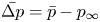 $\bar {\Delta p}=\bar {p}-p_\infty$ and the fluctuation pressure defined as
  $\Delta p_{{fluct}} = p-\bar {p}$, where
  $\bar {p}$ is the time average of
  $p$; in the far field, the fluctuation pressure almost coincides with the sound pressure because
  $\Delta p_{{fluct}}$ satisfies the basic properties of linear acoustic waves as shown in Appendix D. The contour levels are the same for all panels. The mean pressure distributions are similar, although some differences are observed in the wake. In figures 3(b) and 3(f), we observe that the acoustic waves propagate cylindrically from the origin for
  $N_\theta =150$ and
  $0$; the wavelength is larger for
  $N_\theta =150$ than for
  $N_\theta =0$ because the effective diameter of the cylinder is
  $1.8D$ for
  $N_\theta =150$, while it is
  $D$ for
  $N_\theta =0$. However, the acoustic waves are nearly invisible for
  $N_\theta =12$ (figure 3d). This figure shows that the sound is significantly reduced for
  $N_\theta =12$.

Figure 3. Pressure field shown by contour lines of mean pressure  $\overline {\Delta p}=\bar {p}-p_\infty$ (a,c,e) and fluctuation pressure
  $\Delta p_{{fluct}} = p-\bar {p}$ at
  $t=1100$ (b,d,f). Microscopic model with
  $N_r=1$. Red lines,
  ${\Delta }p>0$; green lines,
  ${\Delta }p=0$; blue lines,
  ${\Delta }p<0$. The contour levels are
  $|{\Delta }p|\le 8.0 \times 10^{-4}$ with the increment
  ${\Delta }p_{{inc}}=5.0 \times 10^{-5}$. (a,b)
  $N_{\theta }=150$, (c,d)
  $N_{\theta }=12$, (e,f)
  $N_{\theta }=0$.
Figure 4 shows the time evolutions of pressure measured at  $(r,\theta )=(80,90^\circ )$, the drag
  $F_x$ and the lift
  $F_y$ for the three cases as in figure 3. The drag and lift are calculated as the reaction force of the rate of change of momentum owing to the penalization terms:
 \begin{align} F_i&={-}\int_S f_i \, \textrm{d} A \nonumber\\ &={-}\int_{\partial S} (\rho u_iu_j+p\delta_{ij} -\tau_{ij}) n_j \, \textrm{d} l - {\frac{\textrm{{d}} {}}{\textrm{{d}} {t}}} \int_S \rho u_i \, \textrm{d} A, \end{align}
where  $\boldsymbol {f}$ is the force per unit area owing to the penalization terms,
  $S$ is any region including the cylinder and the porous material, and
  $\boldsymbol {n}$ is the unit outward normal vector on
  $S$. In the following, the region
  $S$ is set to the rectangle
  $[-3D, 12D] \times [-3D, 3D]$ after confirming that the results do not depend on the choice of the region. Nearly sinusoidal oscillations of the pressure are observed for
  $N_r=150$ and
  $0$, while the amplitude and the time period for
  $N_r=150$ are larger than those for
  $N_r=0$. However, the fluctuation pressure is small for
  $N_r=12$, as observed in figure 3(b). The aeroacoustic sound in the present problem is dominated by the time variation of the lift (figure 4c) rather than that of the drag (figure 4b) in the framework of acoustic analogies: we can observe that the amplitude of the lift oscillations is larger for
  $N_r=150$ than
  $N_r=0$; it almost vanishes for
  $N_r=12$; and the time periods of the lift oscillations are the same as those of the fluctuation pressure. We will show how the mean drag and the root-mean-square (r.m.s.) amplitude of lift depend on the number of small cylinders later in this section.

Figure 4. Time evolution of pressure at  $(r,\theta )=(80,90^\circ )$ (a), drag
  $F_x$ (b) and lift
  $F_y$ (c). Microscopic model with
  $N_r=1$. Comparison between
  $N_\theta =150, 12$ and
  $0$.
$0$.
Figure 5 compares the directivity of the sound between  $N_\theta =150, 12$ and
  $0$ for
  $N_r=1$; the r.m.s. amplitudes of the acoustic waves are shown by a polar plot. It shows that the sound for
  $N_\theta =150$ and
  $0$ is dominated by a dipolar component with maximum at
  $\theta \approx \pm 90^\circ$, as is well known for the aeolian tone. However, the directivity for
  $N_\theta =12$, which is magnified in figure 5(b), is not of dipolar nature. It shows that the sound arising from vortex shedding is suppressed nearly completely.

Figure 5. Directivity of r.m.s. amplitude of pressure fluctuations shown by a polar plot. Microscopic model with  $N_r=1$. (a) Comparison between
  $N_{\theta } = 150$ (
 $\bullet$ - red),
  $N_{\theta } = 12$ (
 $+$ - green) and
  $N_{\theta } = 0$ (
 $\times$ - blue); (b) magnified plot of
  $N_{\theta } = 12$.
In figure 6, the acoustic power is plotted against the number  $N_\theta$ of small cylinders in the azimuthal direction. It is calculated at
  $r=80$ as
 \begin{equation} P = \int_0^{2{\rm \pi}} \frac{(\Delta p_{{fluct}})^2}{\rho_\infty c_\infty} r \, \textrm{d} \theta, \end{equation}
while  $23$ observation points at
  $\theta =15^\circ, 30^\circ, \ldots, 345^\circ$ are used to discretize the above integral;
  $\theta =0^\circ$ is excluded because the fluctuation pressure is dominated by hydrodynamic pressure owing to vortices in the wake and the acoustic pressure of the dipolar sound is small. The acoustic power does not change very much for
  $N_\theta \ge 100$; it is approximately five times larger than that for the bare cylinder
  $N_\theta =0$. For
  $N_r=1$, the acoustic power decreases as
  $N_\theta$ decreases for
  $N_\theta \ge 15$. The minimum at
  $N_\theta =12$ is
  $P=5.90\times 10^{-9}$, which is
  $0.36\,\%$ (
 $24.4$ dB reduction) of the bare cylinder and
  $0.064\,\%$ (
 $32.0$ dB reduction) of
  $N_\theta =150$, showing a significant reduction of the acoustic power. The reduction effects are weaker for
  $N_r=2$ and
  $3$ as the minimum acoustic power is
  $25\,\%$ (
 $6.0$ dB reduction) and
  $85\,\%$ (
 $0.7$ dB reduction) of the bare cylinder for
  $N_r=2$ and
  $3$, respectively.

Figure 6. Acoustic power plotted against  $N_{\theta }$. Microscopic model:
  $\bullet$ - red,
  $N_r =1$;
  $+$ - green,
  $N_r = 2$;
  $\times$ - blue,
  $N_r = 3$;
  $\blacksquare$ - black, bare cylinder.
Figure 7 shows contours of vorticity for  $N_\theta =150, 12$ and
  $0$ with
  $N_r=1$. Two instants of opposite phase, one of which is the final time of simulation
  $t=1100$, are shown for each case as the vortex motion is periodic; note that the other instant depends on the case because the time period is different between the three cases. For
  $N_\theta =150$ and
  $0$, vortex shedding behind the cylinder is observed. For
  $N_\theta =12$, however, vortices are not shed just behind the cylinder; it is delayed to
  $x \approx 12$; a nearly steady wake is formed for
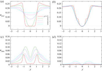
  $0 \le x \lesssim 12$. The flow is blocked by the small cylinders so that a thick boundary layer is formed around the bare cylinder. As a result, the wake is stabilized, for which the details are discussed in § 6. In figure 8, the mean flow and the fluctuation of the streamwise velocity are shown at several positions in the wake. It shows that the mean flow does not change behind the cylinder for
  $N_\theta =12$, while the width of the wake quickly broadens for
  $N_\theta =150$. It also confirms that the fluctuation is small for
  $N_\theta =12$. It is interesting to see that the mean flow and the fluctuation shown in figure 8 are similar to those observed in the experiment (Sueki et al. Reference Sueki, Takaishi, Ikeda and Arai2010) at
  $Re=4.6\times 10^4$ shown in figures 10 and 11 of Sueki et al. (Reference Sueki, Takaishi, Ikeda and Arai2010) in spite of the large difference in the Reynolds number.

Figure 7. Vorticity field shown by contour lines. Microscopic model with  $N_r=1$: red lines,
  ${\omega }>0$; blue lines,
  ${\omega }<0$. The contour levels are
  $|{\omega }|\le 2.0$ with the increment
  $\Delta {\omega }=0.1$. The core cylinder is shown by the filled grey circles, while the outer boundary of the porous material is marked by the black circles. (a)
  $N_{\theta }=150, t=1078$, (b)
  $N_{\theta }=150, t=1100$, (c)
  $N_{\theta }=12, t=1074$, (d)
  $N_{\theta }=12, t=1100$, (e)
  $N_{\theta }=0, t=1087$, (f)
  $N_{\theta }=0, t=1100$.

Figure 8. (a,b) Averaged wake velocity distribution and (c,d) r.m.s. amplitude of wake velocity fluctuation. Microscopic model with  $N_r=1$. (a,c)
  $N_\theta =150$, (b,d)
  $N_\theta =12$.
It is of interest to check how the drag and lift vary with the number of the small cylinders. Figure 9 shows the mean drag coefficient, the r.m.s. amplitude of the lift coefficient and the Strouhal number plotted against  $N_\theta$ for
  $N_r=1, 2$ and
  $3$. They are non-dimensionalized using the outer diameter
  $D_o$ in the left vertical axis, which is suitable for large
  $N_\theta$, and the inner diameter
  $D$ in the right vertical axis, which is suitable for small
  $N_\theta$ as
 $$\begin{gather} C_{D,{{O}}}=\frac{\overline{F_x}}{(1/2)\rho_\infty U_\infty^2 D_o}, \quad C_{L,{{rms,O}}}=\frac{\sqrt{\overline{F_y^2}}}{(1/2)\rho_\infty U_\infty^2 D_o}, \quad St_{{{O}}}=\frac{D_o}{U_\infty T_p}, \end{gather}$$
 $$\begin{gather}C_{D}=\frac{\overline{F_x}}{(1/2)\rho_\infty U_\infty^2 D}, \quad C_{L,{{rms}}}=\frac{\sqrt{\overline{F_y^2}}}{(1/2)\rho_\infty U_\infty^2 D}, \quad St=\frac{D}{U_\infty T_p}, \end{gather}$$
where  $T_p$ is the time period of fluid motion. The drag coefficient and the r.m.s. lift coefficient for the bare cylinder are
  $C_{D}=1.337$ and
  $C_{L,{{rms}}}=0.350$, which are close to the values
  $1.368$ and
  $0.383$ obtained by Ali et al. (Reference Ali, Zaki, Ismail, Muhamad and Mahzan2013) and our previous results
  $1.332$ and
  $0.364$ in the body-fitted coordinate system and
  $1.300$ and
  $0.350$ by the volume penalization method (Komatsu et al. Reference Komatsu, Iwakami and Hattori2016); for
  $(N_r, N_\theta )=(3150)$ approximately corresponding to the large cylinder of diameter
  $D_o$ and
  $Re=270$, they are
  $C_{D,{{O}}}=1.379$ and
  $C_{L,{{rms,O}}}=0.599$, which are in reasonable agreement with
  $C_{D,{{O}}}=1.358$ and
  $C_{L,{{rms,O}}}=0.559$ obtained by interpolation using the coefficients at
  $Re=250$ and
  $300$ obtained by Rajani, Kandasamy & Majumdar (Reference Rajani, Kandasamy and Majumdar2009). The value of the drag for
  $N_\theta =150$ coincides with that of the bare cylinder of diameter
  $1.8D$, which is shown later in figure 14. The drag for
  $N_\theta >0$ is larger than that of the bare cylinder in the entire range. There is a range of
  $N_\theta$ in which the drag exceeds the value at
  $N_\theta =150$:
  $N_\theta \ge 40$ for
  $N_r=1$,
  $N_\theta \ge 12$ for
  $N_r=2$ and
  $N_\theta \ge 8$ for
  $N_r=3$. The maximum drag coefficient is
  $C_{D,{{O}}}=1.733$ or
  $C_D=3.120$ for
  $(N_\theta, N_r)=(20, 3)$, which is
  $2.3$ times the drag of the bare cylinder. In these ranges, the distance between the small cylinders is large enough to allow the incoming flow to form a wake behind them; as a result, the drag exerted on each small cylinder becomes large. It is pointed out that the drag coefficient for
  $(N_\theta, N_r)=(12, 1)$, for which the acoustic power is minimum, is
  $C_{D,{{O}}}=1.036$ or
  $C_D=1.865$, which is
  $40\,\%$ larger than the drag of the bare cylinder. However, the r.m.s. amplitude of lift coefficient does not increase very much as
  $N_\theta$ decreases from
  $N_\theta =150$. It decreases and nearly vanishes to
  $C_{L,{{rms,O}}} < 0.0072$ or
  $C_{L,{{rms,O}}} < 0.013$ for
  $12 \le N_\theta \le 20$ at
  $N_r=1$, which corresponds to the significant reduction of the acoustic power. The Strouhal number does not change significantly for
  $N_\theta \gtrsim 30$, which shows that the effective radius of the porous cylinder is the outer diameter
  $D_O$; it increases with decreasing
  $N_\theta$ for
  $N_\theta \lesssim 15$ as the effective radius shifts gradually to that of the inner diameter
  $D$.
$D$.

Figure 9. (a) Mean drag coefficient, (b) r.m.s. amplitude of lift coefficient and (c) Strouhal number plotted against  $N_{\theta }$. Microscopic model:
  $\bullet$ - red,
  $N_r =1$;
  $+$ - green,
  $N_r = 2$;
  $\times$ - blue,
  $N_r = 3$;
  $square$ - black, bare cylinder.
4. Results: macroscopic model
In this section, we show the results obtained for the macroscopic model. Figure 10 compares the fluctuation pressure field between three values of permeability:  $\eta =10^{-3}$, at which the porous material can be regarded as a rigid body;
  $\eta =10$, at which the acoustic power is minimum; and
  $\eta =10^3$, at which the porous material can be ignored (the case of the bare cylinder). This figure is similar to figure 3 showing the fluctuation pressure field for the microscopic model. In fact, figure 3(a) and figure 10(a) correspond to the case of the large cylinder of diameter
  $1.8D$, while figure 3(c) and figure 10(c) correspond to the case of the bare cylinder. However, there is a difference between the states of the minimum acoustic power: although the amplitude of the fluctuation pressure at
  $\eta =10$ is small, weak acoustic waves propagating cylindrically can be recognized in figure 10(b) as the amplitude of the sound is larger than that in figure 3(b).

Figure 10. Pressure field shown by contour lines of fluctuation pressure  $\Delta p_{{fluct}} = p-\bar {p}$ at
  $t=1100$. Macroscopic model. The line colours and the contour levels are the same as in figure 3. (a)
  $\eta =10^{-3}$, (b)
  $\eta =10$, (c)
  $\eta =10^3$.
Figure 11 shows the acoustic power  $P$ plotted against permeability
  $\eta$. The values of
  $P$ at
  $\eta =10^{-3}$ and
  $10^3$ coincide with those at
  $N_\theta =150$ and
  $0$ for the microscopic model, respectively. The acoustic power increases slightly as
  $\eta$ increases from
  $\eta =10^{-3}$. It decreases for
  $0.2 < \eta <10$ taking the minimum at
  $\eta =10$. The acoustic power increases monotonically with
  $\eta$ for
  $\eta > 10$. The minimum value at
  $\eta =10$ is
  $P=3.85\times 10^{-7}$, which is
  $4.1\,\%$ (
 $13.8$ dB reduction) of
  $\eta =10^{-3}$ and
  $22\,\%$ (
 $6.5$ dB reduction) of the bare cylinder. This value of
  $P$ is much larger than the minimum obtained for the microscopic model. This point will be examined in the next section.

Figure 11. Acoustic power plotted against permeability  $\eta$. Macroscopic model.
Figure 12 shows the directivity of the sound for  $\eta =10^{-3}, 10$ and
  $10^{3}$. The directivity nearly coincides with that of the microscopic model (figure 5) for
  $\eta =10^{-3}$ and
  $10^{3}$. However, the directivity at
  $\eta =10$ is also dominated by the dipolar component in contrast to that of
  $N_\theta =12$ in figure 5. This is understood by the flow field behind the cylinder. Figure 13 compares the vorticity field in the wake of the cylinder between the three values of
  $\eta$. The boundary layer on the cylinder surface is thicker for
  $\eta =10$ than for
  $\eta =10^{-3}$ and
  $10^3$ as in the case of
  $N_\theta =12$ in the microscopic model (figure 7b). However, the vortex shedding is only slightly delayed in comparison to the case of the microscopic model. The size of the vortices and the frequency of vortex shedding are close to those for the large cylinder (
 $\eta =10^{-3}$). However, the effective radius of the cylinder is close to that of the bare cylinder (
 $\eta =10^3$). These combined effects make the acoustic power small, although the reduction rate is smaller than the microscopic model. Figure 14 shows the mean drag coefficient, the r.m.s. amplitude of the lift coefficient and the Strouhal number plotted against the permeability. The drag at
  $\eta =10^{-3}$ coincides with that of the large cylinder. The drag increases with the permeability for
  $10^{-3} < \eta < 1$. Then it decreases monotonically for
  $1< \eta < 10^3$, reaching the value for the bare cylinder at
  $\eta =10^3$. The drag coefficient at the minimum acoustic power (at
  $\eta =10$) is
  $C_{D,{{O}}}=1.086$ or
  $C_D=1.955$, which is
  $44\,\%$ larger than that of the bare cylinder. The amplitude of the lift coefficient takes a minimum at
  $\eta \approx 10$ for which the acoustic power is minimum; however, the minimum of
  $C_{L,{rms}}$ is
  $C_{L,{{rms,O}}}=0.102$ or
  $C_{L,{{rms}}}=0.184$ which is much larger than that in the microscopic model. The Strouhal number increases smoothly for
  $1 \lesssim \eta \le 10^3$, which suggests that the effective radius of the porous cylinder decreases from
  $D_O$ to
  $D$.
$D$.

Figure 12. Directivity of r.m.s. amplitude of pressure fluctuations shown by a polar plot. Macroscopic model. Comparison between  $\eta = 10^{-3}$ (
 $\bullet$ - red),
  $\eta = 10$ (
 $+$ - green) and
  $\eta = 10^3$ (
 $\times$ - blue).

Figure 13. Vorticity field shown by contour lines. Macroscopic model. The line colours, contour levels and the cylinders are the same as in figure 7. (a) 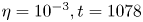 $\eta =10^{-3}, t=1078$, (b)
  $\eta =10^{-3}, t=1100$, (c)
  $\eta =10, t=1081$, (d)
 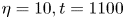 $\eta =10, t=1100$, (e)
  $\eta =10^{3}, t=1086$, (f)
  $\eta =10^{3}, t=1100$.

Figure 14. Mean drag coefficient, r.m.s. amplitude of lift coefficient and Strouhal number plotted against permeability  $\eta$. Macroscopic model.
Figure 15 shows the effects of the thickness of the porous material on the minimum acoustic power. The minimum acoustic power is slightly larger than that of the bare cylinder for  $0< h<0.2D$. However, it decreases with the thickness for
  $0.15D< h<0.5D$. It is of some interest to optimize the thickness for sound reduction; however, it is postponed for a future work because prior to this, we should find the relation between the microscopic and macroscopic models.

Figure 15. Minimum acoustic power plotted against thickness  $h$ of porous material.
5. Relation between microscopic and macroscopic models
In § 4 we showed that the minimum of the acoustic power obtained for the macroscopic model is much larger than that obtained for the microscopic model (§ 3). In this section, we introduce a modified macroscopic model and show that the results obtained for it are consistent with those obtained for the microscopic model. Figure 16(a) shows the microscopic model with  $N_r=1$. Because we have set the outer small cylinders at
  $r=0.9D-0.5d_s=0.885D$, it is not appropriate to model the whole region between the small cylinders and the core cylinder as porous material when
  $N_r=1$. Thus we introduce a modified model as shown in figure 16(b). In this model, there is a region occupied by a fluid between the core cylinder and the porous material of thickness
  $h$ which models the small cylinders. This modified model is expected to be closer to the microscopic model with
  $N_r=1$.

Figure 16. (a) Microscopic model with  $N_r=1$ and
  $N_\theta =32$ and (b) modified macroscopic model.
Figure 17 shows the acoustic power plotted against the permeability for the modified macroscopic model. The results with four values of thickness are compared:  $h=0.4D, 0.2D, 0.1D$ and
  $0.03D$. Note that
  $h=0.4D$ corresponds to the original macroscopic model. As the thickness decreases, the minimum acoustic power decreases, while the value of
  $\eta$ at the minimum also decreases. The minimum acoustic power for
  $h=0.03D$ and
  $0.1D$ is
  $7.74\times 10^{-9}$ at
  $\eta =0.6$ and
  $1.13\times 10^{-8}$ at
  $\eta =2.5$, respectively, which are the same order of magnitude as that of the microscopic model.

Figure 17. Acoustic power plotted against permeability  $\eta$. Modified macroscopic model:
  $square$ - black,
  $h=0.4D$;
  $\bullet$ - red,
  $h=0.2D$;
  $+$ - green,
  $h=0.1D$;
  $\times$ - blue,
  $h=0.03D$.
Figure 18 shows the mean drag plotted against the permeability. The maximum of the mean drag decreases and shifts to smaller  $\eta$ as the thickness decreases. The maxima for
  $h=0.03D$ and
  $0.1D$ are close to that of the microscopic model. The wake behind the cylinder is stabilized as observed in figure 19, which shows the vorticity field for
  $h=0.03D$ at
  $\eta =0.6$ and is similar to that of the microscopic model with
  $(N_r, N_\theta )=(12, 1)$ (figure 7d).

Figure 18. Drag plotted against permeability  $\eta$. Modified macroscopic model:
  $square$ - black,
  $h=0.4D$;
  $\bullet$ - red,
  $h=0.2D$;
  $+$ - green,
  $h=0.1D$;
  $\times$ - blue,
  $h=0.03D$.

Figure 19. Vorticity field shown by contour lines. Modified macroscopic model with  $h=0.03D$ and
  $\eta =0.6$. The line colours, contour levels and the cylinders are the same as in figure 7.
The above results for  $h=0.03D$ and
  $0.1D$ suggest that the modified macroscopic model is closely related to the microscopic model. To compare the results obtained with the two models, we resort to the estimate of the intrinsic permeability of fibrous media obtained by the theory of homogenization (Berdichevsky & Cai Reference Berdichevsky and Cai1993; Boutin Reference Boutin2000; Auriault, Boutin & Geindreau Reference Auriault, Boutin and Geindreau2009)
 \begin{equation} K_{{pT}} ={-}\frac{1}{4} \left[\log \beta + \frac{1-\beta^4}{2(1+\beta^4)} \right] R_e^2. \end{equation}
In the above equation,  $K_{{pT}}$ is the P estimate of the transverse intrinsic permeability,
  $\beta =R_s/R_e$,
  $R_s$ is the radius of small cylinders modelling fibres and
  $R_e$ is the external radius of a fluid shell which contains a small cylinder. The intrinsic permeability is related to the permeability
  $\eta$ and the viscosity
  $\mu$ through
 \begin{equation} \eta=\frac{\rho_\infty c_\infty K_{{pT}}}{\mu D},\end{equation}
in the present scaling. Naturally, we can set  $R_s=d_s/2$. The porosity
  $\phi$ in the above estimate is related to
  $\beta$ by
  $\phi =1-\beta ^2$, which implies that
  $\beta ^2$ is the ratio of the area
  $S_{{cyl}}$ occupied by the small cylinders to the area
  $S_{{por}}$ of the porous material. In our microscopic model, we have
  $S_{{cyl}}={\rm \pi} (d_s/2)^2N_rN_\theta$ and
  $S_{{por}}={\rm \pi} h(D_o-h)$, which allow us to express
  $\beta ^2$ by the parameters in the microscopic model:
 \begin{equation} \beta^2=1-\phi=\frac{S_{{cyl}}}{S_{{por}}}=\frac{d_s^2N_rN_\theta}{4h(D_o-h)}. \end{equation}
Substituting (5.1), (5.3) and  $\beta =R_s/R_e$ into (5.2), the permeability in the modified macroscopic model is expressed by the parameters in the microscopic model.
The acoustic power and the drag obtained for the microscopic model are compared with those obtained for the modified macroscopic model as a function of permeability  $\eta$ using the above equations in figure 20; the microscopic models with
  $N_r=1$ and
  $3$ are compared with the modified macroscopic models with
  $h=0.03D$ and
  $0.4D$, respectively. It shows that the results obtained for the two models are in good agreement. In fact, both the acoustic power and the drag obtained for the microscopic model with
  $N_r=1$ nearly collapse with those obtained for the macroscopic model with
  $h=0.03D$ except for a small deviation at
  $\eta \gtrsim 1$, where the corresponding values of
  $N_\theta$ are small. The agreement between the microscopic model with
  $N_r=3$ and the macroscopic model with
  $h=0.4D$ looks slightly worse because variation of the acoustic power in the microscopic model occurs at small
  $N_\theta$ and the minimum of the acoustic power is out of the range of
  $N_\theta$; however, the agreement is satisfactory as the overall trend is the same and the maxima of the drag are close.

Figure 20. Comparison between modified macroscopic and microscopic models. (a,b) Acoustic power, (c,d) mean drag coefficient and (e,f) r.m.s. amplitude of lift coefficient plotted against permeability  $\eta$. (a,c)
  $\times$ - blue, modified macroscopic model with
  $h=0.03D$;
  $\bullet$ - red, microscopic model with
  $N_r=1$; (b,d)
  $square$ - black, (modified) macroscopic model with
  $h=0.4D$;
  $\times$ - blue, microscopic model with
  $N_r=3$.
Some discussions are required on the applicability of equations derived by homogenization in the present problem. At first sight, the small cylinders in the microscopic model are not sufficiently small or the number of them is not sufficiently large in order for the theory of homogenization to be applicable. However, the relation derived from the theory of homogenization works satisfactorily as we see above. This is because the most important assumption in homogenization holds: the Reynolds number based on the small cylinder is  $Ud_s/\nu =4.5$, which is sufficiently small; the flow around the small cylinders can be approximated by the Stokes flow. Therefore, the results support not only that the microscopic and macroscopic models are consistent but also that these two models are valid.
6. Detailed mechanism of sound reduction
In this section, we discuss the mechanism of sound reduction by the porous material in detail based on the results obtained for the modified macroscopic model.
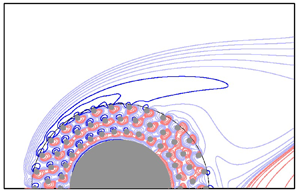
In figure 21, we compare the time-averaged pressure and vorticity fields near the cylinder among the three cases: (i)  $h=0.03D$ and
  $\eta =0.6$ at which the acoustic power is minimum in the modified macroscopic model (figure 21a,b), (ii)
  $h=0.4D$ and
  $\eta =10$ at which the acoustic power is minimum for
  $h=0.4D$ or the original macroscopic model (figure 21c,d) and (iii)
  $h=0.4D$ and
  $\eta =10^{-3}$ which corresponds to the case of the large rigid cylinder of radius
  $0.9D$ (figure 21e,f). At
  $h=0.03D$ and
  $\eta =0.6$, the incoming flow splits into two parts as it attacks the porous material: a part of the incoming flow intrudes into the inside of the porous material forming a jet-like flow shown by the positive vorticity region near
  $r=0.9D$ and the negative vorticity region near
  $r=0.5D$; the rest of the incoming flow forms a boundary layer outside the porous material (figure 21b). The boundary layer outside the porous material separates at
  $\theta \approx 80^\circ$ to form a small separation bubble; however, it reattaches to the surface of the porous material. Alternatively, there is a flow which permeates from the inside of the porous material into its outside behind the cylinder or the wake. As a result, a thick shear layer forms in the wake (figure 21b). The resulting pressure field is nearly constant in the wake (figure 21a), which makes the wake flow nearly steady and leads to significant reduction of the aeroacoustic sound.

Figure 21. Comparison of mean pressure field (a,c,e) and mean vorticity field (b,d,f) near cylinder between three cases: (a,b)  $h=0.03D$ and
  $\eta =0.6$ (minimum acoustic power in the modified macroscopic model), (c,d)
  $h=0.4D$ and
  $\eta =10$ (minimum acoustic power in the original macroscopic model) and (e,f)
  $h=0.4D$ and
  $\eta =10^{-3}$ (large cylinder). The core cylinder is shown by the filled grey semi-circles, while the outer boundary of the porous material is marked by the black semi-circles. In the pressure fields, time average of
  $\Delta p$ is shown by coloured contour lines with the increment
  $\Delta p_{{inc}} = 10^{-3}$. The vorticity fields are shown by contour lines of dyadic contour levels
  $\omega = \pm 0.01 \times 2^{n}$ (
 $n=0, 1, \ldots$): light blue lines,
  $\omega <0, 0 \le n \le 5$; blue lines,
  $\omega <0, n \ge 6$; red lines,
  $\omega >0$. Panel (g) compares the pressure coefficient
  $C_p=\Delta p/((1/2)M_\infty ^2)$ on the outer boundary of the porous material (
 $r=0.9D$) for the three cases.
The acoustic power is also reduced at  $h=0.4D$ and
  $\eta =10$, although the reduction rate is smaller than at
  $h=0.03D$ and
  $\eta =0.6$. At
  $h=0.4D$ and
  $\eta =10$, most portion of the incoming flow permeates into the porous material forming a thick boundary layer from the front side of the core cylinder (figure 21d); the boundary layer develops into a thick shear layer in the wake which is similar to that in figure 21(b). One notable difference is the pressure distribution in the wake: there is non-vanishing pressure gradient in the wake and the pressure on the surface of the porous material is smaller than that at
  $h=0.03$ and
  $\eta =0.6$ as shown by the pressure coefficient
  $C_p=\Delta p/((1/2)M_\infty ^2$ in figure 21(g). As a result, the flow cannot be steady, although unsteady motion is suppressed in comparison to the case of large cylinder (figures 21e,f).
7. Concluding remarks
The effects of the porous material on the aeroacoustic sound generated in a low-Reynolds-number flow past a circular cylinder were studied by direct numerical simulation. Two models were introduced for the porous material: the microscopic model, in which the porous material is a collection of small cylinders, and the macroscopic model, in which the porous material is continuum characterized by permeability. The corrected volume penalization method (Komatsu et al. Reference Komatsu, Iwakami and Hattori2016; Hattori & Komatsu Reference Hattori and Komatsu2017) enabled us to capture aeroacoustic waves of small amplitudes as a solution to the compressible Navier–Stokes equations supplemented by penalization terms without using aeroacoustic analogies or solving additional equations. In the microscopic model, significant reduction of the aeroacoustic sound was found depending on the parameters; maximum reduction was achieved at  $(N_r, N_\theta )=(1, 12)$, which gave
  $24.4$ dB reduction in comparison to the bare cylinder. The vortex shedding behind the cylinder is delayed to the far wake to suppress the unsteady vortex motion near the cylinder, which is responsible for the aeroacoustic sound. In the macroscopic model, sound reduction was not as significant as in the microscopic model when the porous material is attached to the core cylinder; the maximum reduction in comparison to the bare cylinder is
  $6.5$ dB. In the modified macroscopic model, however, a reduction rate comparable to the case of the microscopic model was found when there was a fluid region between the porous material and the core cylinder. The results obtained for the modified macroscopic model were in good agreement with those obtained for the microscopic model converted by the theory of homogenization (Berdichevsky & Cai Reference Berdichevsky and Cai1993; Boutin Reference Boutin2000; Auriault et al. Reference Auriault, Boutin and Geindreau2009), which established not only that the microscopic and macroscopic models are consistent but also that these two models are valid. One of the important findings in the present study is that the reduction effect of the porous material on the aeroacoustic sound depends strongly on the properties of the porous material: it depends not only on the thickness of the porous material but also on the permeability or porosity of the porous material. For instance, the porosity should be in the range
  $0.91 \lesssim \phi \lesssim 0.96$ in order that the sound is reduced more than
  $20$ dB from the bare cylinder.
It is of interest to compare the present results with the experiment by Sueki et al. (Reference Sueki, Takaishi, Ikeda and Arai2010), although the Reynolds number is different. Sueki et al. (Reference Sueki, Takaishi, Ikeda and Arai2010) showed the sound pressure level of the aeroacoustic noise at the vortex shedding frequency is reduced by approximately  $20$ dB and
  $30$ dB in comparison to the bare cylinder and the large cylinder, respectively, while the porosity of the porous materials is larger than
  $97\,\%$. The maximum reduction rate in the present study is comparable to the above values, where a
  $24.4$ dB and
  $32.0$ dB reduction in comparison to the bare cylinder and the large cylinder, respectively, are obtained for the microscopic model; by using the relation (5.3), the porosity at the minimum can be evaluated as
  $\phi =1-\beta ^2=94.9\,\%$, which is smaller than the above value in the experiment. In the modified macroscopic model, however, the porous material is confined at the boundary of the large cylinder; if the region between the core and the large cylinders is regarded as the porous material, as in the original macroscopic model, the value of porosity becomes
  $\phi =98.5\,\%$, which agrees with the experiment. As we have pointed out in § 3, the mean flow and the fluctuation in the wake are also similar to those observed by Sueki et al. (Reference Sueki, Takaishi, Ikeda and Arai2010). Therefore, the essential mechanism of sound reduction is most likely to be the same for the present work and the experiment. This is not surprising because it is the tonal noise at the vortex shedding frequency that is significantly reduced in the study by Sueki et al. (Reference Sueki, Takaishi, Ikeda and Arai2010).
However, we should further check several important differences between the present case and that of Sueki et al. (Reference Sueki, Takaishi, Ikeda and Arai2010): the Reynolds number based on the small cylinder is  $4.5$ in the present work, which implies that the flow around the small cylinders is the Stokes flow; however, the Reynolds number based on the thickness of the small-scale structures in the porous material in the study by Sueki et al. (Reference Sueki, Takaishi, Ikeda and Arai2010) is estimated as
  $Re=O(10^{2\sim 3})$, at which vortices are shed from these structures. The flow is assumed as two-dimensional in the present case, although three-dimensional effects should be important in high-Reynolds-number flows with three-dimensional structures of the porous material in the experiment by Sueki et al. (Reference Sueki, Takaishi, Ikeda and Arai2010). In the present work, the presence of the fluid region between the porous material and the core cylinder is important, while there is no such region in the experiment. One layer of small cylinders in our microscopic model is sufficient for significant reduction of the aeroacoustic sound; this is probably owing to the low Reynolds number of the flow. It is possible that the three-dimensional unsteady flow in the small structures of the porous material acts as eddy viscosity so that their overall effects are similar to the present case, which is of great interest to study as a future work. Unfortunately, it is hopeless to perform DNS based on the microscopic model for three-dimensional flows at the Reynolds numbers of the experiments because of the huge computational costs; comparison of the two models in three-dimensional moderate-Reynolds-number flows would be feasible, which is one of our future works. The present results have shown that the microscopic model can be replaced by the macroscopic model, for which the numerical costs are low, at least in the low-Reynolds-number flows; this is a starting point for validating the macroscopic model in general, although more works are required to establish the validity for higher-Reynolds-numberflows.
It is well known that sound absorption and reduction of the sound speed occur in porous materials (Cervera et al. Reference Cervera, Sanchis, Sánchez-Pérez, Martínez-Sala, Rubio, Meseguer, López, Caballero and Sánchez-Dehesa2002). These effects, if present, are correctly taken into account in the microscopic model as long as the porous material is correctly modelled by the small cylinders; in the macroscopic model, they are also taken into account at least in the low-frequency or long-wave approximation under which Darcy's law is derived (Fellah & Depollier Reference Fellah and Depollier2000) because the most important term of volume penalization in our method coincides with Darcy's law. In the present case, however, these effects are not significant because it is the pressure distribution owing to vortices and the cylinders, which is much larger than the acoustic waves near the core cylinder, that is responsible for the sound generation; in fact, the time variation of the pressure distribution arising from vortices and the cylinders produces acoustic waves under the effect of retarded time. Sound absorption and reduction of the sound speed can be important when multiple objects are placed in the flow so that the acoustic waves generated near one object reflect from other objects covered by the porous material. It would be of interest to investigate these effects together with the effects of elasticity in the porous material, which have been neglected in the microscopic model; this should be another future work.
When the two models are validated for DNS of the aeroacoustic sound in a flow involving a porous material, they can be used to optimize and design the shape and porosity of the porous material to minimize the aeroacoustic sound. In particular, numerical simulation based on the macroscopic model requires smaller costs for the parameter study than experiments as the total computational time required for the macroscopic model was 22.0 hours, while it was 58.7 hours for the microscopic model on one node (40 cores) of PRIMERGY at the Institute of Fluid Science, Tohoku University; the time increases to 738.8 hours for the microscopic model with the minimum grid spacing  $\Delta x_{{min}}/D=1.90\times 10^{-3}$ used for checking numerical accuracy ( Appendix B). The adjoint-based optimization can be implemented to the macroscopic model and is expected to explore new possibilities for sound reduction. Reduction of the aeroacoustic sound is an important issue in many engineering applications, as described in § 1. Although the present method focused on the effects of the porous material, it would be useful to pursue other possibilities as actual implementation of a reduction method can be prohibited by a number of reasons including cost, durability and robustness of the effects; it should be pointed out that in the present method, the drag increases and the actual size of the cylinder becomes large by using the porous material, which can be a disadvantage in some applications. In this regard, various methods proposed for suppression of vortex-induced oscillation can also be effective for reduction of the aeroacoustic sound because they reduce the fluctuation of the force exerted on the object in general (Wong & Kokkalis Reference Wong and Kokkalis1982; Blevins Reference Blevins1990).
Acknowledgements
Numerical calculations were performed on PRIMERGY at the Institute of Fluid Science, Tohoku University.
Declaration of interest
The authors report no conflict of interest.
Appendix A. Computational grids
We adopt a rectangular grid system with non-uniform spacings because the computational domain should be large enough to capture acoustic waves in the far field and the grid spacing should be fine enough to resolve boundary layers on the rigid bodies. As performed by Komatsu et al. (Reference Komatsu, Iwakami and Hattori2016), the computational domain is divided into four regions of different grid spacings (figure 22a): (i) the boundary layer region  $R_{bl}$, in which the grid size is smaller than
  $0.005D$ and
  $0.01D$ in the microscopic and macroscopic models, respectively, (ii) the flow region
  $R_f$, in which the grid size is smaller than
  $0.1D$ (in both models), (iii) the sound region
  $R_s$, in which the grid size is smaller than
  $D$ and (iv) the buffer region
  $R_{bf}$. The grid spacings in the first three regions are small enough to resolve boundary layers in
  $R_{bl}$, vortices in
  $R_f$ and acoustic waves in
  $R_s$. In the buffer region
  $R_{bf}$, the grid spacing is prescribed to be large so that the acoustic waves are damped by the stretching of the spacing and thereby numerical reflection at the outer boundaries, which is small but does occur in spite of the non-reflecting boundary conditions, is reduced sufficiently. Table 1 lists the minimum grid size and the boundary layer and flow regions of the microscopic and macroscopic models. The sound region is larger than the square
  $|x|,|y| \le 100$, while the whole region is
  $|x|,|y| \le 1000$. The grid spacing is stretched smoothly, as shown in figure 22(b), as a function of grid index. As a result, the whole region is covered as shown in figure 22(c); in this figure, the magnitude of the
  $x$ coordinate is shown in log scale as a function of grid index, while the inset shows the
  $x$ coordinate in linear scale near the cylinder.

Figure 22. Computational grids: (a) set-up of computational grids; (b) grid spacing as a function of index along  $x$ axis; and (c)
  $x$ coordinate as a function of index along
  $x$ axis. In panel (c), the magnitude of the
  $x$ coordinate is shown in log scale, while the inset shows the
  $x$ coordinate near the cylinder in linear scale.
Table 1. Grid parameters. The minimum grid size and the coordinates are non-dimensionalized by  $D$.
$D$.

Appendix B. Numerical accuracy of DNS of microscopic model
It is important to check the accuracy of DNS in the microscopic model because the porous material is a collection of small cylinders of radius  $d_s=0.03$, which demands sufficiently high resolution. First, the no-slip boundary conditions at the small cylinders are checked in figure 23, which shows the distributions of the magnitude of velocity
  $|\boldsymbol {u}|/M_\infty$. In figure 23(a), the distribution is shown by contours. It is confirmed that the magnitude decreases quickly to zero near the small cylinders located at
  $(x, y)=(0, 0.885), (\pm 0.443, 0.766)$ and
  $(-0.766, 0.443)$; the other small cylinders are not visualized because they are in the region where the magnitude is small. This supports that the no-slip boundary conditions are satisfied at the small cylinders. Figure 23(b) shows the distributions of
  $|\boldsymbol {u}|/M_\infty$ along the three lines
  $x=0, -0.4418$ and
  $-0.7651$ passing through the small cylinders located at
  $(x, y)=(0, 0.885), (-0.443, 0.766)$ and
  $(-0.766, 0.443)$; it is pointed out that the lines do not always pass exactly through the centres of the small cylinders; the closest grid line is chosen for each cylinder. It is observed that the velocity decreases quickly to zero at the positions of the small cylinder which are centred at
  $y=0.885, 0.766$ and
  $0.443$, with intervals of width
  $0.03$. It is also confirmed that the boundary layers are captured with approximately seven grid points.

Figure 23. Distribution of magnitude of velocity  $|\boldsymbol {u}|/M_\infty$. Microscopic model with
  $(N_r, N_\theta )=(1,12)$. (a) Contours near the core cylinder; (b) distributions along three lines passing through small cylinders.
Figure 24 compares the time histories of pressure at  $(r, \theta )=(80, 90^\circ )$ for
  $(N_r, N_\theta )=(3, 60)$ and
  $(N_r, N_\theta )=(1, 15)$ between three values of minimum grid spacings in the porous material:
  $\Delta x_{{min}}/D=1.90\times 10^{-3}$ (
 $15.8$ grid points in the diameter
  $d_s$),
  $4.75\times 10^{-3}$ (
 $6.3$ grid points) and
  $9.50\times 10^{-3}$ (
 $3.2$ points). They are in good agreement in each case. Although small differences are visible for
  $(N_r, N_\theta )=(1, 15)$, they are small in magnitude as the amplitude of the fluctuation pressure is approximately
  $4\times 10^{-6}$, which is approximately
  $1.3\,\%$ of that for
  $(N_r, N_\theta )=(3, 60)$. Table 2 compares the acoustic power calculated for the two cases:
  $P_1$ for
  $(N_r, N_\theta )=(3, 60)$ and
  $P_2$ for
 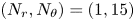 $(N_r, N_\theta )=(1, 15)$. It is pointed out that the latter is close to the minimum of the acoustic power. We observe that accuracy is sufficient for the two cases; the difference in
  $P_1$ between
  $\Delta x_{{min}}/D=1.9\times 10^{-3}$ and
  $4.75\times 10^{-3}$ is
  $0.3\,\%$. Although the relative errors in
  $P_2$ are higher than those in
  $P_1$ (
 $4.4\,\%$ between
  $\Delta x_{{min}}/D=1.9\times 10^{-3}$ and
  $4.75\times 10^{-3}$), the sound is significantly reduced in this case so that the errors are apparently amplified by the small magnitude of the acoustic power. Therefore, the minimum grid size is fixed to
  $\Delta x_{{min}}/D=4.75\times 10^{-3}$ in the microscopic model.

Figure 24. Dependence of time evolution of pressure at  $(r, \theta )=(80, 90^\circ )$ on minimum grid size. Microscopic model: (a)
  $(N_r, N_\theta )=(3, 60)$; and (b)
  $(N_r, N_\theta )=(1, 15)$.
Table 2. Dependence of acoustic power on minimum grid size. Microscopic model.

Appendix C. Dependence on numerical porosity in macroscopic model
The numerical porosity  $\phi _n$, which appears in the penalization term in the conservation of mass (2.2), was fixed to
  $\phi _n=0.98$ in the macroscopic and modified macroscopic models. It is important to check whether this choice gives correct results. It would be legitimate to impose that
  $\phi _n$ coincides with the value
  $0.1$ for rigid bodies at
  $\eta =10^{-4}$ and the penalization term vanishes (
 $\phi _n=1$) at
  $\eta \to \infty$. One such equation is
 \begin{equation} \phi_n=\frac{1}{1+9(\eta_r/\eta)}, \quad \eta_r=10^{{-}4},\end{equation}
(figure 25), while there are many other possibilities.

Figure 25. Relation between permeability  $\eta$ and numerical porosity
  $\phi _n$ of porous material in macroscopic model: black solid line,
  $\phi _n=0.98$; red dashed line, (C1).
Figure 26 compares the acoustic power obtained with fixed numerical porosity  $\phi _n=0.98$ with that obtained by using (C 1). The two results are nearly equal (note that a few data are missing for the case using (C 1)), which shows that the results obtained with fixed numerical porosity are sufficiently accurate. It is pointed out that good agreement is observed not only for large permeability at which the difference in
  $\phi _n$ is small but also for small permeability at which the difference is large (figure 25). In fact, the value of
  $\phi _n$ does not affect the accuracy of DNS as long as the wavelength of the acoustic waves is large compared to the size of the rigid bodies (Komatsu et al. Reference Komatsu, Iwakami and Hattori2016; Hattori & Komatsu Reference Hattori and Komatsu2017).

Figure 26. Acoustic power plotted against permeability  $\eta$. Macroscopic model. Comparison between two different relations between numerical porosity
  $\phi _n$ and
  $\eta$:
  $square$ - black,
  $\phi _n=0.98$;
  $\bullet$ - red, (C1).
Appendix D. Properties of fluctuation pressure
In this appendix, we show that the fluctuation pressure satisfies properties of linear acoustic waves in the far field, which confirms that it nearly coincides with the sound pressure. The two-dimensional linear acoustic waves are expressed in the far field as
 \begin{equation} p-p_\infty \approx \frac{A}{r^{1/2}} \cos \theta \sin [2{\rm \pi} f (t -r/c_0) + \phi_0 ], \end{equation}
when a dipolar sound source is oscillating sinusoidally. Figure 27 shows the dependence of the amplitude of fluctuation pressure on the distance from the origin for the microscopic model of 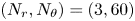 $(N_r, N_\theta )=(3, 60)$ and
  $(N_r, N_\theta )=(1, 15)$;
  $\Delta p_{{fluct}}$ is measured at
  $2.5 \le r/D \le 80$, while the directions
  $\theta =90^\circ$ for
  $(N_r, N_\theta )=(3, 60)$ and
  $\theta =120^\circ$ for
  $(N_r, N_\theta )=(1, 15)$ are close to the directions of the maximum amplitude. In both cases, the amplitude in the far field is nearly proportional to
  $r^{-1/2}$, which is a property of the linear acoustic waves in two dimensions; in fact,
  $r^{-1/2}$-dependence is observed in
  $r/D \gtrsim 15$ for
  $(N_r, N_\theta )=(3, 60)$ and in
  $r/D \gtrsim 40$ for
  $(N_r, N_\theta )=(1, 15)$; for small
  $r$, the fluctuation pressure is dominated by the hydrodynamic pressure.

Figure 27. Amplitude of fluctuation pressure plotted against distance from origin. Microscopic model: (a)  $(N_r, N_\theta )=(3, 60)$ and (b)
  $(N_r, N_\theta )=(1, 15)$. The observation points are
  $\theta =90^\circ$ (a) and
  $\theta =120^\circ$ (b) with
  $r/D=2.5, 5, 10, 20, 30, 40, 50, 60, 70$ and
  $80$. The black lines are proportional to
  $r^{-1/2}$.
Figure 28 compares the pressure  $p-p_\infty$ and the fluctuation pressure
  $\Delta p_{{fluct}}$ for the microscopic model of
  $(N_r, N_\theta )=(3, 60)$; not only the observation points in the far field but also those in the near field are considered:
  $r/D =2.5, 5, 10, 20$ and
  $40$ with
  $\theta =90^\circ$. The pressure
  $p-p_\infty$ at
  $r/D=2.5$ and
  $5$ is negative showing that it is affected significantly by the hydrodynamic pressure which has a negative mean value. The time average of the fluctuation pressure
  $\Delta p_{{fluct}}$ is zero by definition (figure 28b). In figure 28(c), the fluctuation pressure
  $\Delta p_{{fluct}}$ is multiplied by
  $r^{1/2}$ and the retarded time
  $t-r/c_0$ is used as the horizontal axis. The curves for
  $r/D=2.5$ and
  $5$ are larger in amplitude than those for
  $r/D \ge 10$ which nearly collapse. This also confirms that the fluctuation pressure is affected significantly by the hydrodynamic pressure for
  $r/D=2.5$ and
  $5$, while in the far field
  $r/D \gtrsim 15$, the fluctuation pressure satisfies the property of the linear acoustic waves as further confirmed below.

Figure 28. Comparison between pressure  $p-p_0$ and fluctuation pressure
  $\Delta p_{{fluct}}$. Microscopic model with
  $(N_r, N_\theta )=(3, 60)$. The observation points are located at
  $r/D=2.5, 5, 10, 20$ and
  $40$ with
  $\theta =90^\circ$: (a)
  $p-p_0$; (b)
  $\Delta p_{{fluct}}$; (c)
  $\Delta p_{{fluct}}$ multiplied by
  $r^{1/2}$. In panel (c), the horizontal axis is replaced by the retarded time
  $t-r/c_0$.
Figure 29 shows the time evolution of the fluctuation pressure in the far field for the microscopic model of  $(N_r, N_\theta )=(3, 60)$ and
  $(N_r, N_\theta )=(1, 15)$;
  $\Delta p_{{fluct}}$ is measured at
  $r/D=20, 40, 60$ and
  $80$, while the direction is
  $\theta =90^\circ$ for which the Doppler effect arising from the uniform flow vanishes. In figures 29(a) and 29(c), the amplitude and the phase of the fluctuation pressure depends on
  $r$. In figure 29(b), however, the curves collapse when
  $\Delta p_{{fluct}}$ is multiplied by
  $r^{1/2}$ and the retarded time
  $t-r/c_0$ is used as the horizontal axis; it confirms that the fluctuation pressure nearly coincides with the sound wave propagating linearly from the origin for
  $r/D \ge 20$. Similar collapse except for
  $r/D=20$ is also observed in figure 29(d), which shows that the fluctuation pressure at
  $r/D=20$ is affected by pseudo sound because the sound is significantly reduced in this case. In both cases, the fluctuation pressure observed at
  $r/D=80$ is sufficiently close to the sound pressure.

Figure 29. Time evolution of fluctuation pressure  $\Delta p_{{fluct}}$. Microscopic model: (a,b)
  $(N_r, N_\theta )=(3, 60)$; and (c,d)
  $(N_r, N_\theta )=(1, 15)$. In panels (a) and (c),
  $\Delta p_{{fluct}}$ observed at
  $r/D=20, 40, 60$ and
  $80$ with
  $\theta =90^\circ$ are shown. In panels (b) and (d), the fluctuation pressure is multiplied by
  $r^{1/2}$ to compensate for the dependence on
  $r$, while the horizontal axis is replaced by the retarded time
  $t-r/c_0$.