1. Introduction

Governments providing pensions and insurers selling annuities encounter the so-called longevity risk, which is the risk of paying more than anticipated due to unexpected mortality improvement. To assess the probable extent of future mortality decline, an extensive amount of research has been conducted in the past 20 years in the area of mortality projection. In the literature, most of the work is related to the Lee & Carter (Reference Lee and Carter1992) method and its various extensions (e.g. Lee, Reference Lee2000). Because of analytical intractability of these models, simulation methods represent a practically viable means to measure the variability of mortality changes and so the longevity risk, and have been adopted in many applications (e.g. Kogure & Kurachi, Reference Kogure and Kurachi2010).

Initially, Lee & Carter (Reference Lee and Carter1992) focused only on the error term of the random walk with drift for the mortality index (though they also provided suggestions on how to include the errors of parameter estimation). Li et al. (Reference Li, Lee and Tuljapurkar2004) further incorporated the estimation error of the drift term. Brouhns et al. (Reference Brouhns, Denuit and Vermunt2002b) took a different approach and generated samples of the parameters from the multivariate normal distribution. On the other hand, Brouhns et al. (Reference Brouhns, Denuit and Van Keilegom2005) considered bootstrapping the number of deaths from the Poisson distribution. Koissi et al. (Reference Lee2006) also examined bootstrapping the residuals to produce pseudo data samples. Renshaw & Haberman (Reference Renshaw and Haberman2008) then provided a comparative study of the last three simulation methods, which tested different model structures, parameter constraints, scale parameters, and distribution assumptions. They suggested that using the multivariate normal distribution to generate samples of the parameters would lead to widely differing prediction intervals under different constraints. They also found that using variable scale parameters and the negative binomial distribution would result in wider prediction intervals when bootstrapping the number of deaths. Moreover, Czado et al. (Reference Czado, Delwarde and Denuit2005) applied Bayesian modelling and Markov chain Monte Carlo (MCMC) simulation to mortality projection.

Under the current regulatory environment that has become more risk based, it is of practical interest to find a probability distribution to depict how actual outcomes may differ from expected. This distribution can be used to compute such risk metrics as standard deviation, variance, and value-at-risk in pricing, hedging, reserving, and capital management. For example, QIS5 Technical Specifications for Solvency II states that “the nature of the risks underlying the insurance contracts could be described by the probability distribution of the future cash flows arising from the contracts”, and that all of process error, parameter error, and model error should be considered. Prudential Standard GPS 320 by Australian Prudential Regulation Authority (2013) also stipulates that the minimum value of insurance liabilities must be the greater of the “75% level of sufficiency” and the “central estimate plus one half of a standard deviation above the mean”. As such, it is important for practitioners to choose suitable simulation methods to generate random samples of future outcomes, from which different probability inferences can be drawn. In particular, uncertainty in parameter estimation needs to be sufficiently allowed for when the portfolio size is small.

In this paper, we carry out a quantitative comparison of all these simulation methods, using population data from New Zealand. Particularly, we apply the Poisson Lee–Carter (LC) model proposed by Brouhns et al. (Reference Brouhns, Denuit and Vermunt2002a). We construct prediction intervals for projected death rates and life expectancy, and pay particular attention to selecting an appropriate data fitting period.

The paper is organised as follows. Section 2 provides an overview of the six simulation strategies. Section 3 presents the results of applying these simulation techniques to the mortality data of New Zealand. Section 4 sets forth our concluding remarks.

2. Simulation Strategies

The Poisson LC model proposed by Brouhns et al. (Reference Brouhns, Denuit and Vermunt2002a) is defined as follows

$$D_{{x,t}} \,\sim\,{\rm Poisson }\left( {{\rm }e_{{x,t}}\ {\rm }m_{{x,t}} } \right),\quad \quad \quad \quad \quad \ln m_{{x,t}} =a_{x} {\plus}b_{x} {\rm }k_{t} $$

in which D _x,t is the number of deaths at age x in year t, e _x,t the corresponding (known) exposure, m _x,t the central death rate, a _x the general mortality schedule, and b _x measures the sensitivity of the log death rate to changes in the mortality index k _t. The mortality index is usually modelled as a random walk with drift, i.e., $$k_{t} =\mu {\plus}k_{{t{\minus}1}} {\plus}{\varepsilon}_{t} $$ where μ is the drift term and ε _t the error term with mean zero and variance σ ². This model offers a natural way to model the number of deaths and avoids the assumption of homoscedastic errors in the original LC method. The maximum likelihood parameter estimates are calculated from an iterative updating scheme (based on Newton’s method), subject to two constraints $$\mathop{\sum}{b_{x} } =1$$ and $$\mathop{\sum}{k_{t} } =0$$ . In the next section, we will check the resulting residuals for the goodness-of-fit and take the most recently observed data as the starting point of projection.

After equation (1) is fitted to the data, the following six simulation strategies are tested:

1. (I) Lee & Carter (Reference Lee and Carter1992) focused on ε _t and used ±2σ to approximate the 95% prediction intervals. Here, assuming $${\varepsilon}_{t} \,\sim\,N{\rm }\left( {{\rm }0{\rm },{\rm }\sigma ^{2} } \right)$$ , we simulate n samples of future k _t via $$k_{t} =\hat{\mu }\,{\plus}\,k_{{t\,{\minus}\,1}} \,{\plus}\,{\varepsilon}_{t} $$ and then obtain values of future death rates using the estimated parameters.

2. (II) Li et al. (Reference Li, Lee and Tuljapurkar2004) assumed $${\varepsilon}_{t} \,\sim\,N{\rm }\left( {{\rm }0{\rm },{\rm }\sigma ^{2} } \right)$$ and simulated n samples of future k _t with $$k_{t} =\hat{\mu }\,{\plus}\,{\rm se}\left( {\hat{\mu }} \right){\rm }\eta \,{\plus}\,k_{{t\,{\minus}\,1}} \,{\plus}\,{\varepsilon}_{t} $$ , where $${\rm se}\left( {\hat{\mu }} \right)$$ was the standard error in estimating μ and $$\eta \,\sim\,N{\rm }\left( {{\rm }0{\rm },{\rm }1{\rm }} \right)$$ . Note that ε _t and η were treated as independent. They then obtained values of future death rates using the estimated parameters.

3. (III) Brouhns et al. (Reference Brouhns, Denuit and Vermunt2002b) adopted a parametric Monte Carlo simulation approach. They first generated a sample of the model parameters $$(a_{x}^{{\left( j \right)}} ,\,\,b_{x}^{{\left( j \right)}} ,\,\,k_{t}^{{\left( j \right)}} )$$ from the asymptotic multivariate normal distribution, in which the mean was approximately taken as the maximum likelihood parameter estimates and the covariance matrix was given by the inverse of the Fisher information matrix. The Cholesky decomposition process was used to produce multivariate random samples. Then they fitted a new time series model to the sampled mortality index $$(k_{t}^{{\left( j \right)}} )$$ and projected it to the future, allowing for the error term of the time series model. Finally, they produced values of future death rates $$(m_{{x,t}}^{{\left( j \right)}} )$$ using the sampled parameters and the projected mortality index. The whole process was repeated to generate n scenarios, i.e., j=1, 2, …, n. Renshaw & Haberman (Reference Renshaw and Haberman2008) also considered incorporating the scale parameter ϕ into the covariance matrix.

4. (IV) Brouhns et al. (Reference Brouhns, Denuit and Van Keilegom2005) implemented a semi-parametric bootstrapping approach. They first bootstrapped a pseudo sample of the number of deaths $$(d_{{x,t}}^{{\left( j \right)}} )$$ from the Poisson distribution with mean d _x,t, the observed number of deaths. They applied equation (1) to this pseudo sample and computed the model parameters $$(a_{x}^{{\left( j \right)}} ,\,\,b_{x}^{{\left( j \right)}} ,\,\,k_{t}^{{\left( j \right)}} )$$ . Then they fitted a new time series model to the mortality index $$(k_{t}^{{\left( j \right)}} )$$ of the pseudo sample and projected it to the future, taking into account the error term of the time series model. Correspondingly, they generated values of future death rates $$(m_{{x,t}}^{{\left( j \right)}} )$$ with the computed parameters and the projected mortality index of the pseudo sample. The entire process was repeated many times to produce n scenarios, i.e., j=1, 2, …, n. Wang & Lu (Reference Wang and Lu2005) also took a similar approach (with the binomial distribution) to calculate the standard error of the parameter estimates. On the other hand, Renshaw & Haberman (Reference Renshaw and Haberman2008) sampled from the fitted Poisson distribution (with mean $$\hat{d}_{{x,t}} $$ ) instead.

5. (V) Koissi et al. (Reference Koissi, Shapiro and Hognas2006) suggested the use of residual bootstrapping. First, they resampled, with replacement, the deviance residuals $$(r_{{x,t}}^{{\left( j \right)}} )$$ based on the fitted Poisson distribution. Then they used the inverse formula to turn these resampled residuals into a pseudo sample of the number of deaths $$(d_{{x,t}}^{{\left( j \right)}} )$$ , and applied equation (1) to this pseudo sample and computed the model parameters $$(a_{x}^{{\left( j \right)}} ,\,\,b_{x}^{{\left( j \right)}} ,\,\,k_{t}^{{\left( j \right)}} )$$ . They fitted a new random walk with drift to the mortality index $$(k_{t}^{{\left( j \right)}} )$$ of the pseudo sample and projected it to the future, allowing for the error term $${\varepsilon}_{t} $$ . Finally, they generated values of future death rates $$(m_{{x,t}}^{{\left( j \right)}} )$$ with the computed parameters and the projected mortality index of the pseudo sample. The whole process was repeated to give n scenarios, i.e., j=1, 2, …, n. Here, we follow the inverse formula used by Renshaw & Haberman (Reference Renshaw and Haberman2008), as it complies with the principle in Efron & Tibshirani (Reference Efron and Tibshirani1993), such that it gives a pseudo sample of the number of deaths (instead of the fitted number of deaths).

6. (VI) Czado et al. (Reference Czado, Delwarde and Denuit2005) applied Bayesian modelling and MCMC simulation (the Gibbs sampler and Metropolis–Hastings algorithm) to project mortality. The major step of Bayesian analysis is to find the posterior distribution of the unknown parameters and quantities given the data. In principle, the posterior density function can be derived from $$f\left( {\bitheta \!\mid\!{\bf D}} \right)\propto\,f\left( {\bf D\!\mid\!\bitheta } \right){\rm }f\left( \bitheta \right)$$ where θ denotes the unknown parameters and quantities and D means the data. As this problem is mathematically intractable, one can perform MCMC simulation to generate samples from the posterior distribution. Similar to Czado et al. (Reference Czado, Delwarde and Denuit2005) and also Kogure et al. (Reference Kogure, Kitsukawa and Kurachi2009), we choose the prior distributions below:

$$a_{x} \,\sim\,N{\rm }\left( {{\rm }0{\rm },{\rm }\sigma _{a}^{2} } \right)$$

$$b_{x} \,\sim\,N{\rm }\left( {{\rm }{\textstyle{{\rm 1} \over {{\rm number\ of\ age\ groups}}}}{\rm },{\rm }\sigma _{b}^{2} } \right)$$

$$\mu \,\sim\,{N}{\rm }\left( {{\rm }\mu _{0} {\rm },{\rm }\sigma _{\mu }^{2} } \right)$$

$${\varepsilon}_{t} \,\sim\,N{\rm }\left( {{\rm }0{\rm },{\rm }\sigma ^{2} } \right)$$

$$\sigma ^{{{\minus}2}} \,\sim\,{\rm Gamma }\ \left( {\alpha {\rm },{\rm }\beta } \right)$$

In effect, (I) considers only the random error of projecting the mortality index, while (II) also allows for the fact that different data samples would give rise to different estimates of the drift term. On the other hand, (III) to (V) incorporate both the error of estimating the model parameters due to sampling fluctuation and the random error of projecting the mortality index. For (VI), Bayesian analysis automatically includes all these errors via the prior distributions. Roughly speaking, (I) caters for process error only, while (II) to (VI) take both process error and parameter error (or parameter uncertainty) into account. In terms of programming and computation, (I) and (II) are fairly straightforward and do not require much computation time, whereas (III) to (VI) are generally much more demanding and time-consuming. In our analysis below, the former takes 15 minutes or so to run, but the latter ones can take quite a few hours to even a couple of days.

We run at least 5,000 iterations (i.e. n=5,000) for each strategy, from which we can obtain the sample means, sample standard deviations, and 95% prediction intervals for projected death rates and life expectancy. To perform simulations, we utilise the software R for (I) to (V) and WinBUGS (Spiegelhalter et al., Reference Spiegelhalter, Thomas, Best and Lunn2003) for (VI). Note that some practitioners may find the MCMC simulation process in (VI) too tedious to implement, as it involves complex scientific programming. The specialised software WinBUGS provides an alternative, in which the programming language is relatively easy to use (e.g. Li, Reference Li2014). For demonstration purposes, we adopt WinBUGS to carry out MCMC simulation. The simulation process, however, can still take up to a couple of days to run. If greater flexibility is required, one may develop MCMC algorithms from scratch, but this calls for significant expertise in building the models and writing the codes. Note also that vague priors are further tested, such as multiplying $$\sigma _{a}^{2} $$ and $$\sigma _{b}^{2} $$ by 10. The sample means are basically not affected, and the resulting changes in the sample variances are immaterial.

3. Simulation Results

The number of deaths and exposed to risk data of New Zealand for 1948–2008, by sex and single year of age, are collected from the Human Mortality Database (2012). As noted in Li (Reference Li2010, Reference Li2013), the linearity of the mortality index in the LC structure is an important property for projecting the overall mortality decline and makes the projection a sensible and straightforward exercise. Moreover, the fundamental drivers of mortality improvement have changed significantly for the recent decades, and it is often preferable to include only the most recent and relevant data periods. Figure 1 shows the mortality indices computed from applying equation (1) to the whole set of data, in which there is a prominent change in the slope in around 1985 for both sexes. This change is found to be broadly in line with the emergence of old-age improvement during that period of time. As such, following Li (Reference Li2010), we select the starting year 1985 for all the projections below. In that paper, the selection was based on the change in the slope, the stability of b _x’s, and the R ² values of testing the linearity of the k _t series. In addition, as the death rates from age 90 onwards are rather volatile due to small exposures, we exclude these data from our analysis and adopt the Coale & Guo (Reference Coale and Guo1989) method to “close out” the life table when computing life expectancy.

Figure 1 Mortality indices for the data period 1948–2008.

There are two main reasons behind the use of New Zealand data for testing the simulation methods. First, its population size is much smaller than those of the United Kingdom and the United States, the data of which are often used in mortality projection studies. The smaller sample size means higher uncertainty in parameter estimation, which makes it important to incorporate parameter error into the simulation process. Second, data of insurance portfolios and pension plans are generally much less than population data, and the experience of a relatively small country is more comparable to those of the largest portfolios and plans.

The estimated parameters based on the fitting period 1985–2008 are plotted in Figure 2. The a _x estimates display the typical shape of the mortality schedule. For the b _x estimates, there are three peaks at early childhood, around age 20, and age 60, which refer to the highest sensitivity to the general trend of mortality decline. Moreover, as expected, the k _t series are reasonably linear, and this feature helps justify the use of the random walk with drift. The corresponding standardised deviance residuals are then shown in Figure 3. Overall, these residuals are randomly distributed against age, calendar year, and cohort year. The absence of significant unusual patterns in the residuals indicates that the Poisson LC model (equation (1)) can be deemed as being able to capture the main characteristics of the data. The randomness of the residuals also provides a strong basis for using the residual bootstrapping method (V).

Figure 2 Parameter estimates for the data period 1985–2008.

Figure 3 Standardised deviance residuals for the data period 1985–2008. Note: The empty cells refer to positive residuals and the marked ones refer to negative residuals.

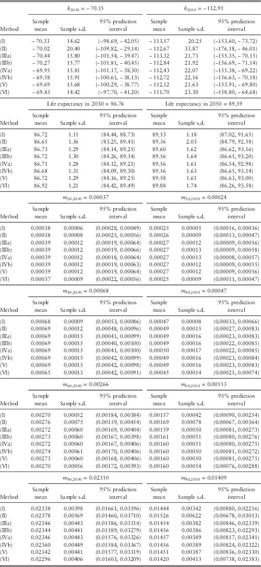
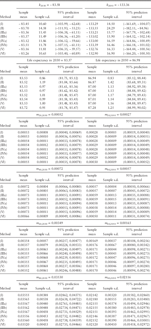
Provided with the parameter estimates, we apply the six simulation methods (I) to (VI) to generate samples of future death rates and life expectancy and construct 95% prediction intervals. As mentioned earlier, we further divide each of (III) and (IV) into two cases: (IIIa) without the scale parameter versus (IIIb) with the scale parameter; (IVa) using the observed number of deaths as the Poisson parameter versus (IVb) using the fitted Poisson distribution. The scale parameter is a measure of over-dispersion and its incorporation would lead to higher variability if it is larger than 1. Moreover, for (III) to (V), we do not fit a new time series model (e.g. ARIMA models) but simply a new random walk with drift in each iteration, since the mortality index samples are largely linear. It should also be noted that all the parameters and future values are sampled coherently under (VI).

Tables 1 and 2 list the projected values (central estimates calculated from the maximum likelihood estimates of the parameters and the projected mortality index), sample means, sample standard deviations, and 95% prediction intervals for future mortality index, (period) life expectancy at birth, and death rates at different ages in 2030 and 2050. Figure 4 plots the sample means and 95% prediction intervals for future values in 2050. We have made a number of observations as below:

1. (1) The sample means agree closely with the projected values based on maximum likelihood.

2. (2) The widths of the 95% prediction intervals are on average around 3.9 times the standard deviations. This ratio is the same as that of a normal distribution.

3. (3) Compared with all the other methods, (I) clearly leads to smaller variances and narrower prediction intervals. This result is a direct consequence of allowing for only the random error term of the random walk with drift. For life expectancy, the magnitude of the differences appears to increase over time in the projections.

4. (4) For the mortality index and life expectancy, it can be seen that (II) gives rise to the largest variances and widest prediction intervals. For the death rates, (II) produces larger variances and wider prediction intervals at older ages but the results are opposite at younger ages, when compared with the other methods (except (I)).

5. (5) The results of (IIIa) and (IIIb) are very close. Because the scale parameters for females and males are only 1.09 and 1.11, there is effectively not much difference between the two variations.

6. (6) There does not appear to be any material difference between using the observed number of deaths and the fitted number of deaths as the Poisson parameter. The figures produced by (IVa) and (IVb) are very similar.

7. (7) Overall, the results of (III) to (V) are highly comparable. This agreement seems to further suggest that the Poisson LC model (equation (1)) provides a satisfactory fit to the data. Brouhns et al. (Reference Brouhns, Denuit and Van Keilegom2005) made a similar comment when they compared (IIIa) and (IVa).

8. (8) The figures computed from (VI) are quite close to those from (III) to (V). For the mortality index, death rates at older ages, and life expectancy, (VI) tends to give larger variances and wider prediction intervals than (III) to (V) later in 2050, but the situation is reversed earlier in 2030. On the other hand, for the death rates at younger ages, (VI) tends to produce smaller variances and narrower prediction intervals in both periods.

9. (9) Figure 5 displays the sampled distributions of life expectancy at birth in 2050. It can be seen that the shapes of the distributions are very similar for (III) to (V), which agree with the observations above.

10. (10) It is interesting to observe in Figure 5 that there is a small extent of skewness in the sampled distributions of life expectancy. While the distributions generated by (I) and (II) are negatively skewed, those by (III) to (VI) are slightly positively skewed. We realise that the former case actually becomes more negatively skewed over time during the projection period, whereas the latter changes from being negatively skewed to positively skewed gradually. Li et al. (Reference Li, Lee and Tuljapurkar2004) and Li (Reference Li2013) demonstrated the same effects as the former case when they adopted (II). This negative skewness in life expectancy appears to be driven by the fact that changes in the mortality index are the only source of uncertainty allowed for and that these changes follow the normal distribution, which means that the projected death rates are then lognormally distributed and have positive skewness. On the other hand, for (III) to (VI), there is also uncertainty of the other parameters, and the aggregate effects on skewness are mixed and less clear-cut.

Figure 4 (a) 2.5^th percentiles, sample means, and 97.5^th percentiles for future mortality index, life expectancy at birth, and death rates in 2050 (females).

Figure 4 (b) 2.5^th percentiles, sample means, and 97.5^th percentiles for future mortality index, life expectancy at birth, and death rates in 2050 (males).

Figure 5 (a) Sampled distributions of life expectancy at birth in 2050 (females).

Figure 5 (b) Sampled distributions of life expectancy at birth in 2050 (males).

Table 1 Projected values, sample means, sample standard deviations, and 95% prediction intervals for future mortality index, life expectancy at birth, and death rates in 2030 and 2050 (females).

Table 2 Projected values, sample means, sample standard deviations, and 95% prediction intervals for future mortality index, life expectancy at birth, and death rates in 2030 and 2050 (males).

It should be noted that (I) incorporates only the random error of projecting the mortality index and ignores the existence of parameter error, which unavoidably lead to an understatement of variability in mortality movements. In contrast, all the other methods also take parameter error into account, but through different ways: (II) focuses on the estimation error of the drift term of the random walk process, while (III) to (VI) allow for the estimation error of the original model parameters. Undoubtedly, (III) to (VI) offer a more precise and sophisticated mechanism for integrating different sources of errors. Nevertheless, (II) has two potential advantages over the others. First, its computation time is much shorter and the programming required is less demanding. Second, as old-age improvement has become more important, and since (II) generates future death rates at old ages and mortality index with greater variability, this method tends to give a higher estimate of variability for such aggregate measures as life expectancy and present value of an annuity at retirement ages. It means that the resulting allowance for uncertainty would be more conservative, which may be preferred by certain pension and annuity providers. In summary, the optimal choice depends on the requirements of the analysis and the experience and preference of the user. Ideally, if time permits and resources are available, a practitioner could test different simulation methods and compare the results, so as to gain a better understanding of the underlying uncertainty of mortality changes.

Finally, there are three more things to note. First, as discussed above, the difference between (IIIa) and (IIIb) is minimal because the estimated scale parameter is close to 1. (It was calculated to be 1.386 for UK male pensioner data in Renshaw & Haberman, Reference Renshaw and Haberman2008). This may not be the case for other countries or populations. Second, we suggest earlier that the close agreement of the figures from (III) to (V) may be an indication of the good fit of the Poisson LC model (equation (1)) to the data. We suspect that for the situation where the model fit is unsatisfactory (e.g. there are unusual patterns in the residuals), the results produced by different simulation methods may differ considerably. In those cases, the differences may be reduced if some modifications are made to the model to first improve the data fitting. Third, though in this paper, the projection is performed for 42 years based on only 24 years of data, this work is for demonstration purposes only. In practical applications, the convention is that the maximum length of the projection period is taken approximately the same as the length of the fitting period (e.g. Booth et al., Reference Booth, Maindonald and Smith2002).

4. Concluding Remarks

In this paper, we provide a quantitative comparison of six simulation strategies for mortality projection using the Poisson LC model. These strategies include considering the error term of the mortality index only, including the parameter error of the drift term, simulating the parameters from the multivariate normal distribution, bootstrapping the number of deaths from the Poisson distribution, bootstrapping the deviance residuals of the fitted model, and Bayesian MCMC simulation. We apply these different methods to New Zealand mortality data and find that (a) the first method produces the lowest variability estimates; (b) the second method largely gives the highest variability estimates; and (c) the last four methods lead to similar results. We recognise that the second method involves much less programming and computation demand than the last four methods and that the final choice depends on the specific requirements and preference of the user. We also emphasise the importance of having a satisfactory model fit before carrying out any simulation of future values.

For future research, we are exploring the possibility to further incorporate the model error. One option is to make use of the Bayesian framework to consider two or more models at the same time and set a prior probability for each model, as suggested in Cairns (Reference Cairns2000). It would also be informative to conduct a similar quantitative study for other mortality model structures and data sets. Moreover, D’Amato et al. (Reference D’Amato, Di Lorenzo, Haberman, Russolillo and Sibillo2011) recently proposed the use of stratified sampling for handling heterogeneity between clusters within a population. It would be interesting to see how this approach could improve the residual bootstrapping process in the cases where there exists dependence between the residuals for certain sub-groups of the population under study. Other work considering the dependence structure in the residuals includes Debón et al. (Reference Debón, Montes, Mateu, Porcu and Bevilacqua2008, Reference Debón, Martínez-Ruiz and Montes2010) and D’Amato et al. (Reference D’Amato, Haberman, Piscopo and Russolillo2012).