


1. Introduction
Coherent jets are one of the most striking features of planetary atmospheres and oceans, and appear ubiquitous in a wide range of geophysical, as well as astrophysical and magnetized plasma, systems. They have received much attention over the past few decades, from the early work of Rhines (Reference Rhines1975) to a vast range of articles in the recent comprehensive collection of Galperin & Read (Reference Galperin and Read2019), exploring aspects of jet formation, structure and transport properties using a variety of theoretical, numerical and experimental approaches. Despite the range and depth of investigations, however, a general theoretical framework with predictive capability under a wide range of forcing conditions remains elusive, and fundamental issues such as energy equilibration and the process of jet merger are still not well understood.
One of the simplest settings in which to study jets is the two-dimensional barotropic vorticity equation with varying background potential vorticity. The system is amenable to numerical integration, where any unresolved process, such as gravity wave breaking or baroclinic instability, can be represented by a prescribed random forcing. Two important length scales can be identified: the Rhines scale,  $ {L_{Rh}}=\sqrt {U/\beta }$, where
  $U$ is a characteristic velocity and
  $\beta$ is the background planetary vorticity gradient, (Rhines Reference Rhines1975; Williams Reference Williams1978); and
  $ {L_{{\varepsilon }}}={{\varepsilon }}^{1/5}\beta ^{-3/5}$, where
  ${{\varepsilon }}$ is the energy input rate, which can be related to the scale at which anisotropy becomes important (Maltrud & Vallis Reference Maltrud and Vallis1991; Vallis & Maltrud Reference Vallis and Maltrud1993; Sukoriansky, Dikovskaya & Galperin Reference Sukoriansky, Dikovskaya and Galperin2007). Studies have been moderately successful in describing the parameter values for which strong jets emerge, and the general properties of the associated turbulent energy spectrum. In particular, on the potential vorticity staircase, a limiting case in which potential vorticity is perfectly mixed in a piecewise constant profile (McIntyre Reference McIntyre1982; Marcus Reference Marcus1993; Peltier & Stuhne Reference Peltier and Stuhne2002), the relation between Rhines scale and jet separation was made explicit in Dritschel & McIntyre (Reference Dritschel and McIntyre2008) and Dunkerton & Scott (Reference Dunkerton and Scott2008) for straight, regularly separated jets. A further key result of Scott & Dritschel (Reference Scott and Dritschel2012) and Scott & Tissier (Reference Scott and Tissier2012) is that this strong jet limit first emerges when the ratio
  $ { {L_{Rh}}/ {L_{{\varepsilon }}}}$ becomes sufficiently large, numerically above a value of approximately 6. In this paper, we refer to such a regime as the ‘strong-stair limit’. This limit corresponds approximately to the zonostrophic regime discussed in Galperin et al. (Reference Galperin, Sukoriansky, Young, Chemke, Kaspi, Read and Dikovskaya2019) for barotropic flow, with the strong-stair limit being approached at somewhat larger values of
  $ { {L_{Rh}}/ {L_{{\varepsilon }}}}$ than the zonostrophic regime. The conceptual model in which the potential vorticity staircase arises naturally from general mixing processes applies far beyond the barotropic system, however, and has proved a powerful tool in the understanding of the ubiquity of jets in planetary atmospheres and oceans.
While successful, single-layer models necessarily omit consideration of many detailed aspects of real geophysical flows, such as vertical shear and variations in horizontal temperature and static stability. Another branch of numerical investigation has focussed on the more realistic, but much harder situation described by two-layer or fully three-dimensional flows. These introduce two main complications over the single-layer case: (i) a deformation length scale describing the cross-over between rotation and stratification dominated flow; (ii) resolved forcing mechanisms such as baroclinic instability or fully three-dimensional convection. The simplest system to capture both effects is the two-layer system, which has received much attention over many years (Panetta Reference Panetta1993; Thompson & Young Reference Thompson and Young2007; Esler Reference Esler2008; Berloff, Kamenkovich & Pedlosky Reference Berloff, Kamenkovich and Pedlosky2009; Zurita-Gotor, Blanco-Fuentes & Gerber Reference Zurita-Gotor, Blanco-Fuentes and Gerber2014; Williams & Kelsall Reference Williams and Kelsall2015). When a free surface is included, the two-layer system in fact admits both internal and external deformation radii, both of which may influence the cascade of energy from small to larger scales. With more complete vertical structure, studies have considered various aspects of jet development, such as the dependence of jet scaling on planetary parameters (Chemke & Kaspi Reference Chemke and Kaspi2015; Liu & Schneider Reference Liu and Schneider2015), the vertical structure of jets in deep atmospheres (Heimpel, Gastine & Wicht Reference Heimpel, Gastine and Wicht2016) or the development and variability of jets in atmospheres and oceans (Arbic et al. Reference Arbic, Müller, Richman, Shriver, Morten, Scott, Sérazin and Penduff2014; Shevchenko & Berloff Reference Shevchenko and Berloff2015; Robert, Rivière & Codron Reference Robert, Rivière and Codron2017), among many others. However, the greatly increased complexity of these systems severely complicates the development of a more general theory along the lines of the single-layer case.
As an intermediate step, it is possible to consider the dynamics introduced by (i) without the complications of (ii), while remaining within the simple two-dimensional framework of single-layer flow. An appropriate system is the quasi-geostrophic shallow-water model, which includes a parameter  $ {L_D}$ representing the finite deformation length. The model is obtained as the limit of
  $Ro \ll Fr^{2} \ll 1$, of the usual shallow-water model, where
  $Ro$ is the Rossby number and
  $Fr$ is the Froude number (e.g. Pedlosky Reference Pedlosky1979; Vallis Reference Vallis2006). In this system, forcing must still be included in a prescriptive way, and may be considered (as in the barotropic model) as representing the dynamical effects of unrepresented processes such as convection or baroclinic instability without unduly complicating the dynamics. The simplifying assumption of the mid-latitude
  $\beta$-plane is again useful. Generalization to the full shallow-water system and spherical geometry is possible (Cho & Polvani Reference Cho and Polvani1996; Scott & Polvani Reference Scott and Polvani2007), but the effect of the latitudinal variation of
  $ {L_D}$ (Okuno & Masuda Reference Okuno and Masuda2003; Theiss Reference Theiss2004) and the peculiarities of dynamics in the tropics (e.g. Kitamura & Ishioka Reference Kitamura and Ishioka2007; Scott & Polvani Reference Scott and Polvani2008) make a systematic analysis of this system harder than on the mid-latitude
  $\beta$-plane.
While it was noted in Okuno & Masuda (Reference Okuno and Masuda2003) and Theiss (Reference Theiss2004) that a small deformation radius  $ {L_D}$ may prevent the formation of well-defined zonal jets, early studies of quasi-geostrophic shallow-water turbulence typically lacked both the spatial resolution and temporal extent needed for a detailed analysis of jets across a variety of parameter ranges. As in the barotropic case, to obtain strongly mixed potential vorticity it is necessary to use weak forcing acting over long time scales. The reduction of the dynamical time scale at small
  $ {L_D}$ and the need to include
  $ {L_D}$ in the range of resolved spatial scales places severe numerical constraints on the problem. The richness of the dynamics and the need for high spatial resolution were illustrated in Dritschel & McIntyre (Reference Dritschel and McIntyre2008). For these reasons, even the basic question of how the emergence of strong jets depends on the length scales
  $ {L_D}$,
  $ {L_{Rh}}$, and
  $ {L_{{\varepsilon }}}$ remains unanswered, although calculations reported in Scott & Dritschel (Reference Scott and Dritschel2019) indicate a role for the parameter
  $ {L_{Rh}}/ {L_{{\varepsilon }}}$, but with the strong-stair limit approached more quickly at small
  $ {L_D}$. In fact, the calculations reported below indicate that at small
  $ {L_D}$ strong jets emerge already for values
  $ {L_{Rh}}/ {L_{{\varepsilon }}}\sim 3$, well before their counterparts in barotropic flows. Part of the reason they have not been recognized previously is that extensive latitudinal meandering obscures their form in the traditional zonal mean.
Because of the extensive meandering of jets, previous estimates of jet spacing based on simple  $x$-independent flows (Dritschel & McIntyre Reference Dritschel and McIntyre2008; Dunkerton & Scott Reference Dunkerton and Scott2008, summarized in § 3.1) are likely to be inaccurate in practice. One of the main aims of the current paper, therefore, is to extend such estimates to the more typical case of jets that meander extensively in latitude.
The introduction of the parameter  $ {L_D}$ means that the total energy of the system splits into kinetic and potential components. In a forced-dissipative system, and with typical choices for the large-scale dissipation mechanism, neither kinetic nor potential energy can be determined from the global energy equation. This further complicates a priori estimates of the jet spacing
  $ {L_j}$ in terms of
  $ {L_{Rh}}$, where
  $ {L_{Rh}}$ is often most naturally based on the root-mean-square (r.m.s.) velocity, or kinetic energy. A second main aim of the paper, therefore, is to obtain a constraint on the partition of energy between kinetic and potential contributions that will enable such a priori estimates to be made.
The remainder of the paper is organized as follows. In § 2 we define the governing equations of the system, the principal length scales and dimensionless parameters and recall the properties of energy equilibration that may be deduced independently of jet formation. In §§ 3 and 4, we present the main scaling results of the paper, the spacing of strong meandering jets in the strong staircase limit, and corresponding constraints on the kinetic and potential energies. In § 5, we compare the predictions of jet spacing and energy partition with a series of numerical experiments; the experiments also make clearer the region of parameter space where strong staircases can be obtained. In § 6, we conclude with some general remarks and discuss briefly the more complex flow structures – vortices, irregular meanders and loops – that limit the accuracy of the scaling relations.
2. Governing equations and physical parameters
The quasi-geostrophic shallow-water system on the mid-latitude  $\beta$-plane can be expressed as an evolution equation for the potential vorticity,
  $q$
$q$
 $$\begin{gather} q_t + J(\psi,q) = F + D, \end{gather}$$
 $$\begin{gather}q -\beta y = (\nabla^{2} - {L_D^{{-}2}})\psi, \end{gather}$$
where  $\psi$ is the streamfunction,
  $\beta$ is the background potential vorticity gradient and
  $F$ and
  $D$ are forcing and dissipation functions. It differs from the two-dimensional barotropic system only through the introduction of the Rossby deformation length,
  $ {L_D}$. If we assume that the three length scales
  $ {L_D}$,
  $ {L_{Rh}}$ and
  $ {L_{{\varepsilon }}}$ are (i) much smaller than the domain scale,
  $ {L_0}$, and (ii) much larger than the forcing scale
  $ {L_f}$ and the scale of enstrophy dissipation, then we are left with a system that is described entirely in terms of the two independent dimensionless parameters
  $ { {L_{Rh}}/ {L_{{\varepsilon }}}}$ and
  $ { {L_{Rh}}/ {L_D}}$. Either of these may be replaced by the third combination,
  $ {L_{{\varepsilon }}}/ {L_D}$. This approach can be compared with that of Scott & Tissier (Reference Scott and Tissier2012) for the barotropic,
  $ {L_D}\rightarrow \infty$, system, which considered the effect of
  $ {L_f}$ as a third length scale. In that paper it was shown that the basic dependence of jet structure on
  $ { {L_{Rh}}/ {L_{{\varepsilon }}}}$ persists even up to the point when
  $ { {L_{Rh}}/ {L_f}}\sim 1$, and the usual inverse energy cascade is absent. With finite
  $ {L_D}$ but small
  $ {L_f}$, we can similarly consider the approximate location of the boundary between strong and weak jets in the two-dimensional parameter space spanned by
  $ { {L_{Rh}}/ {L_{{\varepsilon }}}}$ and
  $ { {L_{Rh}}/ {L_D}}$.
In (2.1), a common and natural choice of energy dissipation, and one used to obtain a stationary state in the barotropic case, is a linear (Rayleigh) friction on the velocity field, for which  $D=-r\zeta$, where
  $\zeta$ is the vorticity. Assuming that the forcing
  $F$ increases the total energy at a constant rate,
  ${{\varepsilon }}$, the domain average of (2.1) gives the energy equation
 \begin{equation} \frac{{\textrm{d}} {\mathcal{E}}}{{\textrm{d}}t}={{\varepsilon}}-2r{\mathcal{T}}, \end{equation}
where  $ {\mathcal {E}}$ is the total energy and
  $ {\mathcal {T}}$ is the kinetic energy of the system. Unlike the barotropic case, where
  $ {\mathcal {E}}= {\mathcal {T}}$, (2.3) places no a priori bound on the system. As noted in Scott & Dritschel (Reference Scott and Dritschel2013), kinetic energy may equilibrate at any value
  $ {\mathcal {T}}\le {{\varepsilon }}/2r$, while total energy may continue to grow at a rate
  ${{\varepsilon }}-2r {\mathcal {T}}$. If we define the Rhines scale as
  $ {L_{Rh}}=\sqrt {U/\beta }$ with
  $U=\sqrt {2 {\mathcal {T}}}$, we find that it is bounded a priori but not known precisely. In § 4, we show that it is possible to take advantage of the jet structure in the staircase limit to obtain an additional relation between kinetic and potential energy that guarantees equilibration of
  $ {\mathcal {T}}$ at the value
  $ {\mathcal {T}}={{\varepsilon }}/2r$.
The quasi-geostrophic shallow-water system also has a natural representation of thermal relaxation, in which the dissipation operator takes the form  $D=\kappa {L_D^{-2}}\psi$, where
  $\kappa$ is the relaxation rate (Smith et al. Reference Smith, Boccaletti, Henning, Marinov, Tam, Held and Vallis2002). With this choice, the energy equation becomes
 \begin{equation} \frac{{\textrm{d}} {\mathcal{E}}}{{\textrm{d}}t}={{\varepsilon}}-2\kappa{\mathcal{P}}, \end{equation}
where  $ {\mathcal {P}}$ is the potential energy. Again, this equation on its own places no a priori bound on the total energy: potential energy may equilibrate at any value
  $ {\mathcal {P}}\le {{\varepsilon }}/2\kappa$, while total energy may continue to grow at a rate
  ${{\varepsilon }}-2\kappa {\mathcal {P}}$. Here, however, because of the property that potential energy is contained in larger-scale flow structures than kinetic energy, the up-scale energy cascade means that if potential energy equilibrates then so too must kinetic energy, though at a level that is not determined by the forcing and dissipation rates (Scott & Dritschel Reference Scott and Dritschel2013). Again, in the strong-stair limit the relation between kinetic and potential energy derived in § 4 may be used to constrain the kinetic energy.
3. Jet spacing in the strong-stair limit
For the simplest case of straight ( $x$-independent) jets in the barotropic limit,
  $ {L_{Rh}}/ {L_D}\rightarrow 0$, Dritschel & McIntyre (Reference Dritschel and McIntyre2008) (hereafter DM08) derived the relation
  $Lj=2\sqrt {3} {L_{Rh0}}$ between jet spacing
  $ {L_j}$ and a Rhines scale
  $ {L_{Rh0}}=\sqrt { {u_{max}}/\beta }$ based on the maximum along-jet velocity,
  $ {u_{max}}$. The relation follows immediately from the result that
  $ {u_{max}}=\tfrac {1}{12}\beta {L_j}^{2}$ for a regular piecewise constant potential vorticity staircase, with step size
  $\beta {L_j}$. The same scaling was obtained by Dunkerton & Scott (Reference Dunkerton and Scott2008) on the sphere asymptotically close to the equator, and is essentially a consequence of the quadratic dependence of angular momentum on latitude.
In the opposite limit of  $ {L_{Rh0}}/ {L_D}\rightarrow \infty$, of interest here, a similar estimate can be derived under the (temporary) assumption of straight jets. Again, for a perfectly mixed, regular staircase the potential vorticity jump across a jet core, separated from adjacent jets by a distance,
  $ {L_j}$, is
 \begin{equation} {\rm \Delta} q = \beta{L_j}. \end{equation}
For small  $ {L_D}$, the velocity profile decays exponentially from the jet core as
 \begin{equation} u(y)={u_{max}} \, \textrm{e}^{-|y|/{L_D}}, \end{equation}
and is illustrated schematically in figure 1(a). Since the potential vorticity jump is equal to the jump in  $-u_y$ across the jet, we have that
  $\beta {L_j} = 2 {u_{max}}/ {L_D}$, giving immediately the relation
 \begin{equation} {L_j}/ {L_{Rh0}} \sim 2 {L_{Rh0}}/{L_D}, \end{equation}
as obtained in DM08 from the calculation of the full staircase solution. That is, the ratio of jet spacing to Rhines scale now grows as  $ {L_D}$ becomes smaller than
  $ {L_{Rh0}}$.

Figure 1. Schematic of (a) straight and (b) meandering jets, illustrating the jet spacing,  $ {L_j}$, equal to the domain length divided by jet number, and the along-jet velocity profile decaying exponentially over a scale
  $ {L_D}$.
The same result can be given in terms of the more usual  $ {L_{Rh}}=\sqrt { {u_{rms}}/\beta }$ by noting that in the limit of small
  $ {L_D}$ nearly all the kinetic energy resides in the jet core. We therefore have that
 \begin{align} {u_{rms}}^{2} & \approx \frac{2}{{L_j}{L_0}}\int_0^{\infty} {u_{max}}^{2} \, \textrm{e}^{{-}2|y|/{L_D}} {\textrm{d} y} {L_0} \nonumber\\ & \approx \frac{{L_D}}{{L_j}}{u_{max}}^{2}, \end{align}
so that
 \begin{equation} {u_{rms}}^{2} = \tfrac{1}{4}{L_D}^{3} {L_j} \beta^{2}, \end{equation}
or
 \begin{equation} {L_j}/ {L_{Rh}} \sim 4 {L_{Rh}}^{3}/{L_D}^{3}. \end{equation}
 As discussed above, a serious limitation of (3.3) or (3.6) is that it holds only for straight,  $x$-independent (zonal) jets. As the examples shown in § 4 illustrate (see e.g. figure 3 below), jets in this limit tend to meander extensively in latitude. Here, guided by the examples from direct numerical simulation, we look for a correction based on the typical length of jet meanders. All other things being equal, a meandering jet in which the along-jet length is a factor
  $1+\alpha$ greater than that of a straight jet will have a total kinetic energy that is also a factor
  $1+\alpha$ greater than that of the straight jet, provided that the radius of curvature of the meanders is larger than
  $ {L_D}$. Here,
  $\alpha$ is the increase in length over the straight jet configuration. We assume here that the meander does not alter the across jet velocity profile, that the kinetic energy is again concentrated in the jet core, and that the maximum jet speed
  $ {u_{max}}$ does not vary along the jet. The latter assumption is partially justified on the grounds that the straight-jet velocity,
  $ {u_{max}}$ depends only on the potential vorticity jump across the jet,
  $ {u_{max}}=\tfrac 12\beta {L_j} {L_D}$. This argument may fail when, for example, two jets become close together.
To estimate the increase in jet length due to meanders, we note that lateral perturbations of the jet position with a radius of curvature of the order of  $ {L_D}$ will tend to project onto Rossby wave modes that will propagate along the jet; i.e. there is a Rossby wave elasticity on scales
  $ {L_D}$ and smaller (DM08). We hypothesize therefore, that meanders will typically increase to fill the region between jets, while maintaining their radius of curvature as large as possible, and always much larger than
  $ {L_D}$. A notional meander configuration is shown schematically in figure 1(b). If we impose the requirement that radius of curvature be as large as permitted geometrically, then the typical jet length in the
  $y$-direction will equal the typical jet length in the
  $x$-direction, resulting in an increase in jet length by an amount
  $\alpha =1$, and therefore a doubling of the kinetic energy in the jet cores.
Following the argument for (3.6), but with kinetic energy increased by a factor of two, leads therefore to the estimate
 \begin{equation} {L_j}/ {L_{Rh}} \sim 2 {L_{Rh}}^{3}/{L_D}^{3}, \end{equation}
the only difference being the pre-factor. Physically, for a given jet number, or jet spacing, the amount of kinetic energy that the meandering potential vorticity staircase can accommodate is double what it would be were the jets straight. Equivalently, meandering jets allow a given amount of kinetic energy to fit into a smaller space than would be possible were the jets straight, and therefore allow a closer jet spacing. Note that, here, the jet separation is taken as the distance between potential vorticity jumps in an appropriate equivalent-latitude, or area-based, sense; that is, the separation that would result were the jets to be straightened out, keeping the areas between them fixed.
To the extent that the only contribution to the kinetic energy comes from the jets, the estimate (3.7) provides a lower bound for the jet spacing, being based on the rearrangement of potential vorticity into a perfect staircase distribution with regularly spaced steps. Any departure from a perfectly regular staircase, either because of incomplete mixing between jet cores, or because of departures from regular spacing, will result in a jet spacing that is wider than the estimate. Conversely, if significant kinetic energy also resides in other flow features, for example in coherent vortices lying between the jets, then this will tend to result in a jet spacing that is closer than the estimate (3.7).
4. Energy partition
As discussed in § 2, it is not generally possible to obtain an a priori estimate for the kinetic energy from the energy equation alone, regardless of whether the dissipation operator represents frictional or thermal dissipation. In the limit of  $ { {L_{Rh}}/ {L_D}}\rightarrow \infty$ and complete mixing of potential vorticity between jets, however, we can follow arguments like those of § 3 to obtain a relation between potential energy and jet spacing, and hence obtain the ratio of kinetic to potential energies.
Temporarily ignoring jet meanders, for the simplest configuration of uniformly spaced straight jets, located at  $y=\pm b, \pm 2b, \ldots$, where
  $b= {L_j}/2$, the potential energy (per unit area)
  $ {\mathcal {P}}_0$ may then be evaluated by integrating in
  $y$ over the interval
  $[0,b]$
 \begin{equation} 2{\mathcal{P}}_0 =\frac{1}{b}\int_0^{b}{L_D^{{-}2}}\psi^{2} \,{\textrm{d} y}. \end{equation}
Making use of (5.4) in DM08, the integral can be evaluated exactly to give
 \begin{equation} 2{\mathcal{P}}_0 = \beta^{2} b^{2} {L_D}^{2} G(b/{L_D}), \end{equation}
where  $G$ is a combination of hyperbolic functions with the property that
  $G(s)\rightarrow \frac 13$ as
  $s\rightarrow \infty$. Thus in the limit of large
  $b/ {L_D}$ of interest here we obtain
 \begin{equation} 2{\mathcal{P}}_0 = \tfrac{1}{3} \beta^{2} b^{2} {L_D}^{2}. \end{equation}
The integral can be simplified at the outset by taking advantage of the approximation that, outside the jet cores,  $\nabla ^{2}\psi \ll {L_D^{-2}}\psi$ and so the potential vorticity anomaly
  $q'=q-\beta y$ is dominated by
  $ {L_D^{-2}}\psi$. Then in the interval
  $[0,b]$
 \begin{equation} \psi \sim {L_D}^{2} \beta y. \end{equation}
 In the case of meandering jets, we can consider a similar calculation but with the upper limit of the integral replaced by  $b+d_m(x)$, where
  $d_m$ represents the departure of the jet location from
  $y=b$ due to the meander, and followed by a second integration in the
  $x$-direction. Now using (4.4) we have
 \begin{equation} 2{\mathcal{P}} \approx \frac{1}{b{L_0}}\int_0^{{L_0}}\int_0^{b+d_m(x)}{L_D}^{2}\beta^{2}y^{2} \, {\textrm{d}}y\, {\textrm{d}}\kern0.06em x. \end{equation}
The integral over  $y$ results in powers of
  $d_m$ up to
  $d_m^{3}$. However, if meanders are random about
  $y=b$ then, in a suitable ensemble average, terms in odd powers of
  $d_m$ must vanish. The remaining even powers give
 \begin{equation} 2{\mathcal{P}} \approx \frac{1}{3} \beta^{2} b^{2} {L_D}^{2} + \beta^{2} {L_D}^{2}\frac{1}{{L_0}}\int_0^{{L_0}} d_m^{2}(x){\textrm{d}\kern0.06em x}. \end{equation}
 The integral over  $x$ depends on the form of the meanders but an idea of its size may be obtained from a consideration of simple cases. For a sinusoidally varying jet of amplitude
  $b$, thus filling the available
  $y$-range, with
  $d_m(x)=b \sin {kx}$, the integral evaluates to
  $\frac 12 {L_0} b^{2}$, regardless of the wavenumber
  $k$. For a square-wave limit, again of amplitude
  $b$, the value doubles to
  $ {L_0} b^{2}$. We thus find that
 \begin{equation} 2 {\mathcal{P}} \approx C \beta^{2} b^{2} {L_D}^{2} = \tfrac 14 C \beta^{2} {L_j}^{2} {L_D}^{2}, \end{equation}
where the constant  $C$ is numerically close to 1:
  $\frac 56$ or
  $\frac 43$ for the sinusoidal and square-wave limits. Thus the jet meanders induce an approximately threefold increase in potential energy over the straight-jet value.
The corresponding straight-jet kinetic energy,  $ {\mathcal {T}}_0$, is just a rearrangement of (3.6) obtained by expanding
  $ {L_{Rh}}$
 \begin{equation} 2{\mathcal{T}}_0=\tfrac{1}{4}\beta^{2} {L_j} {L_D}^{3}. \end{equation}
As was shown in § 3, the corresponding kinetic energy is simply twice the straight-jet value,
 \begin{equation} {\mathcal{T}}=2{\mathcal{T}}_0. \end{equation}
Combining these results, a crude estimate for the ratio of kinetic to potential energy in the meandering case is therefore
 \begin{equation} \frac{{\mathcal{T}}}{{\mathcal{P}}} = \frac{2}{C}\frac{{L_D}}{{L_j}}, \end{equation}
again with  $C$ close to unity. The ratio of kinetic to potential energy decreases with increasing jet separation. We note that this result is not far from that which would be obtained by ignoring jet meanders entirely, with the straight-jet estimate being
 \begin{equation} \frac{{\mathcal{T}}_0}{{\mathcal{P}}_0} = 3\frac{{L_D}}{{L_j}}. \end{equation}
Thus, the effect of jet meanders is simply to reduce the ratio of kinetic to potential energy by a factor of around  $\frac 23$ from that of the straight-jet case, while preserving the inverse scaling with jet separation.
5. Comparison with numerical simulations
5.1. Numerical configuration
We have carried out a range of numerical simulations of (2.1) to test the estimates obtained above. Here we report quasi-stationary simulations with no explicit large-scale dissipation; other simulations with dissipation operators representing frictional and thermal damping, as discussed in § 2, were also performed to verify the quasi-stationary results. With a constant energy input, no damping ( $D=0$) implies that
  $ {L_{Rh}}$ grows slowly as
  $t^{1/4}$ and the flow may be considered as moving gradually through a series of quasi-equilibrium states, punctuated by isolated more rapid changes due to jet mergers. The quasi-stationary simulations have the advantage of not restricting applicability of the results to a particular situation in which either form of damping is the dominant physical mechanism. An additional, practical advantage is that because energy (and hence
  $ {L_{Rh}}$) grows continually, a single integration of the forced undamped equations sweeps out a one-dimensional line in the two-dimensional parameter space. Thus a one-parameter family of numerical integrations can cover the entire parameter space, representing a significant saving in computational resources.
In all calculations, the domain of integration is  $|x|,|y|\le {L_0}/2={\rm \pi}$ with periodic boundary conditions applied in both
  $x$ and
  $y$. Equations (2.1) are integrated from a state of rest,
  $q=\beta y$, at
  $t=0$ and are forced with random isotropic perturbations, delta-correlated in time, in a narrow shell of wavenumbers centred on
  $ {k_f}$, with
  $ {k_f}\gg {k_D}= {L_D}^{-1}$. Beyond this requirement, our results are insensitive to details of the forcing, as may be anticipated from Burgess & Scott (Reference Burgess and Scott2018) where the properties of the emergent vortex population in two-dimensional isotropic turbulence were demonstrated to be broadly independent of forcing correlation time and its distribution in spectral space.
The energy input rate of the forcing is fixed at rate  ${{\varepsilon }}$. Numerical parameters have been chosen carefully to meet the requirements
  $ {L_f}\ll {L_D}\ll {L_{Rh}}$,
  $ {L_j}\ll {L_0}$, with
  $ { {L_{Rh}}/ {L_{{\varepsilon }}}}$ large enough that the strong-stair limit is attained. For the quasi-equilibrium experiments these are
  $ {k_f}=96$,
  $ {k_D}=24$,
  $\beta =1$ and
  ${{\varepsilon }}=2^{a}\times 10^{-8}$ with
  $a=-8,-7,\ldots,-1,0,0.72$ varied across simulations. A grid of size
  $N^{2}$ with
  $N=1024$ is used and a scale-selective bi-harmonic diffusion is included to remove enstrophy at the smallest scales. The relatively modest spatial resolution is partly necessitated by the long length of the integrations in time, with dimensionless run time
  $T\beta / {L_0}$ in the range
  $10^{6}$ to
  $10^{7}$.
5.2. Summary of the jet parameter dependence
To illustrate the relevant region in parameter space, figure 2 shows the two measures of staircase development defined in Scott & Dritschel (Reference Scott and Dritschel2012) vs  $ { {L_{Rh}}/ {L_{{\varepsilon }}}}$ and
  $ { {L_{Rh}}/ {L_D}}$. Simulations begin at
  $t=0$ at the origin, when the flow is at rest and
  $ {L_{Rh}}=0$. The slopes of the lines are determined by the forcing strength through
  $ {L_{{\varepsilon }}}/ {L_D}$. Black/red indicates weak jets and no staircase, blue indicates strong jets and a well-defined staircase; white can be considered as approximately defining the onset of the staircase. In the barotropic limit,
  $ {L_D}\rightarrow \infty$ (Scott & Dritschel Reference Scott and Dritschel2012) established that the strong-stair regime is reached when
  $ { {L_{Rh}}/ {L_{{\varepsilon }}}}$ exceeds approximately 6. Here, we find that for non-zero
  $ { {L_{Rh}}/ {L_D}}$, strong staircasing occurs at progressively smaller values of
  $ { {L_{Rh}}/ {L_{{\varepsilon }}}}$, saturating at an onset value of approximately
  $ { {L_{Rh}}/ {L_{{\varepsilon }}}}\approx 3$ when
  $ { {L_{Rh}}/ {L_D}}$ exceeds one. Jets are predominantly meandering when
  $ { {L_{Rh}}/ {L_D}}>1$, although it should be borne in mind that even when
  $ { {L_{Rh}}/ {L_D}}\ll 1$, jets in this system tend not to be perfectly straight, but rather wavy (see, for example Scott & Dritschel Reference Scott and Dritschel2012).

Figure 2. The degree of staircase development in the two-dimensional parameter space spanned by  $ { {L_{Rh}}/ {L_{{\varepsilon }}}}\ { {L_{Rh}}/ {L_D}}$. Colours indicate the values of the quantities
  $1-I_1/I_2$ and
  $I_3/I_2$ defined in Scott & Dritschel (Reference Scott and Dritschel2012, (4.1) therein), measuring the closeness of fit to a notional perfect staircase, with a value of 1 representing an exact fit.
As an aside, our numerical simulations demonstrate clearly how the inverse cascade at small  $ {L_D}$ proceeds very differently in
  $\beta$-plane and
  $f$-plane turbulence. Whereas on the
  $f$-plane the cascade halts at
  $ {L_D}$, on the
  $\beta$-plane it may proceed further through the mixing of potential vorticity between jets. Essentially, on the
  $f$-plane the cascade is halted isotropically (giving vortices), whereas on the
  $\beta$-plane it is halted in one dimension only (giving narrow jets, but the spacing between jets may continue to grow).
Figure 2 also indicates the difficulty in reaching the region of parameter space required to verify the estimates obtained in § 3, obtained under the assumption that  $ {L_j}/ {L_D}$ and hence
  $ { {L_{Rh}}/ {L_D}}$ is large. Equation (3.7) implies
  $ {L_j}/ {L_D}\sim 2( { {L_{Rh}}/ {L_D}})^{4}$: the fourth power helps, but
  $ { {L_{Rh}}/ {L_D}}$ must still significantly exceed unity, which it does only for the strongest forcing cases. At these stronger forcing levels, on the other hand, the domain scale is eventually reached. In other words, there is a relatively narrow range of
  $ {L_j}$ that can be accommodated in the relation
  $ {L_D}\ll {L_j}\ll {L_0}$ with present computational resources.
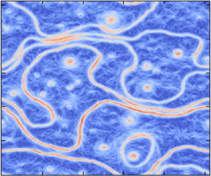
Figure 3 shows three examples of potential vorticity (a) and speed (b), taken from the single simulation with  $a=-2$, of the jet structure during the approach to the strong-stair regime of interest. As time increases, left to right, the energy and hence both
  $ { {L_{Rh}}/ {L_{{\varepsilon }}}}$ and
  $ { {L_{Rh}}/ {L_D}}$ increase at the same rate. Strong jets and a clear staircase structure begin to emerge around
  $ { {L_{Rh}}/ {L_{{\varepsilon }}}}=3$ (middle panel) and become more clearly defined as
  $ { {L_{Rh}}/ {L_{{\varepsilon }}}}$ increases further. Jets meander significantly in all cases. In the strong-stair regime (right panel) the kinetic energy is concentrated increasingly in the meandering jet cores. However, a number of other flow features are also evident, including closed loops resulting from extreme meanders breaking off the main jet, and coherent vortices, which occur both in isolation and within the loops. The formation of loops seen here is not dissimilar to the frequently observed generation of warm core rings from Gulf Stream meanders in the North Atlantic (e.g. Olson Reference Olson1991). Often the loops are formed through a complicated interaction between a strong isolated vortex and a pronounced jet meander. The focus of the current paper is not on such interactions but their presence is noted as a factor that will potentially violate the estimates obtained in § 3 above. In the right panel, approximately 50 %–70 % of the total kinetic energy is contained within the jet cores. We return to discuss the amount of kinetic energy contained within the different coherent structures further below.

Figure 3. Snapshots of the potential vorticity (top row) and speed (bottom row) from the simulation with  $a=-2$, at values of
  $ { {L_{Rh}}/ {L_{{\varepsilon }}}}$ and
  $ { {L_{Rh}}/ {L_D}}$ as indicated in the figure.
5.3. Verification of the estimates
Figure 4(a) shows the values of  $ {L_j}/ {L_{Rh}}$ and
  $ { {L_{Rh}}/ {L_D}}$ from the three simulations with forcing index
  $a=-2,0$, along with the predictions (3.7). The restriction to the strong forcing cases is necessary to ensure
  $ { {L_{Rh}}/ {L_D}}$ (and hence
  $ {L_j}/ {L_D}$) is large enough. Here the jet separation
  $ {L_j}$ has been obtained from an integer count of the number of jets obtained from equivalent-latitude plots of the potential vorticity field, divided by the length of the domain. While this is a relatively crude measure of jet spacing, that neglects along-jet variations, it is at a consistent level of approximation with the assumptions of regular jet spacing underlying the estimates. On average points move up and to the right as time increases, but in the quasi-stationary picture we regard each point as a distinct point in parameter space. Some banding of the data is due to the fact that as
  $ {L_{Rh}}$ increases continuously, the number of jets may remain constant for prolonged intervals between jet mergers.

Figure 4. (a) Jet separation  $ {L_j}/ {L_{Rh}}$ against
  $ {L_{Rh}}^{3}/ {L_D}^{3}$; the prediction (3.7) is indicated by the solid line. (b) Jet separation against
  $( {L_{Rh}}^{3}/ {L_D}^{3})( {L_D}/ {L_{{\varepsilon }}})$.
Considering the crudeness of the approximations leading to (3.7) and the complexities in the evolving flows (e.g. right panel of figure 3), the distribution of jet separations is in some ways surprisingly close to the estimate. Within a single simulation, the distribution of points follows broadly the cubic dependence on  $ { {L_{Rh}}/ {L_D}}$. There is an offset from the estimate that increases at weaker forcing, corresponding to a pre-factor different from unity. Recall that configurations in which jets are unequally spaced or in which potential vorticity is incompletely mixed between steps, but in which kinetic energy remains concentrated in the jet cores, should have wider jet separation than predicted. This would lead to points lying always to the left of the line. Conversely, a low proportion of kinetic energy residing in jet cores would result in a narrower separation than the prediction. Thus an offset to the left may be associated with incomplete or irregular staircasing, while an offset to the right may be associated with a higher fraction of energy contained in non-jet structures such as coherent vortices.
It turns out that the rightward shift of the offset with increasing forcing strength is consistent with an increasing fraction of the kinetic energy contained in the background turbulent flow. Figure 5 shows the amount of kinetic energy, as a fraction of the total, contained within jets, closed loops and coherent vortices for the two cases  $a=-2$ and
  $a=0$. To calculate the kinetic energy, the potential vorticity field is contoured and all contours are identified whose average speed exceeds the r.m.s. value. Of these contours, those that traverse the domain in the
  $x$-direction are classified as belonging to jet cores, contours not traversing but longer than a threshold proportional to
  $ {L_D}$ are classified as loops, while shorter contours are classified as vortices. The kinetic energy in each structure is then computed as the squared speed integrated over the structure. Note that the calculation of jet separation is based on equivalent latitude, in which both jets and loops are considered on an equal footing; indeed loops result from jet meanders that pinch off and may recombine with the original jet at any time. While for
  $a=-2$ most kinetic energy is indeed contained within jets and loops, this is no longer the case for
  $a=0$. The stronger forcing in the latter case essentially results in a much more variable and complex flow. An example is shown in figure 6, which illustrates in particular the substantial fraction of kinetic energy contained in coherent vortices at progressively higher forcing strength for a given value of
  $ { {L_{Rh}}/ {L_{{\varepsilon }}}}$.

Figure 5. Fraction of the total kinetic energy contained with distinct flow features: jets which traverse the domain in the  $x$-direction, jets which form closed (non-traversing) loops, and isolated vortices.

Figure 6. Snapshots of the flow speed from the simulations with  $a=-2$,
  $a=0$ and
  $a=0.72$, (left to right) at values of
  $ {L_D}/ {L_{{\varepsilon }}}$ as indicated in the figure;
  $ {L_{Rh}}/ {L_{{\varepsilon }}}=3.5$ in all cases.
The greater kinetic energy fraction contained within vortices may be partly explained in phenomenological terms. In particular, vortex formation may be related to the separation between the anisotropy scale  $ {L_{{\varepsilon }}}$ and deformation radius
  $ {L_D}$. Whereas at large
  $ {L_D}$, Rossby waves become important when the inverse energy cascade reaches the scale
  $ {L_{{\varepsilon }}}$ (Maltrud & Vallis Reference Maltrud and Vallis1991), at small
  $ {L_D}$, the inverse energy cascade is more typically associated with the formation of strong coherent vortices at the scale
  $ {L_D}$ (Tran & Dritschel Reference Tran and Dritschel2006). A decrease in the kinetic energy fraction contained within the jets compared with vortices might therefore be expected as the ratio
  $ {L_{{\varepsilon }}}/ {L_D}$ increases, as can be seen moving left to right in figure 6. A simple correction to the original prediction (3.7) may be envisioned that takes into account an additional dependence on
  $ {L_{{\varepsilon }}}/ {L_D}$. While we lack a theory for such a correction, figure 4(b) shows the simplest possibility introducing a linear factor into the scaling relation for the jet separation, which improves the collapse of the data, at least for the
  $a=-2$ and
  $a=0$ cases. The collapse could be improved still further using a correction
  $( {L_{{\varepsilon }}}/ {L_D})^{\alpha }$ with
  $\alpha >1$, but it would require significantly more data to determine
  $\alpha$ empirically to any degree of accuracy.
We note that our other main assumption that the structure of the jet meanders are such that the  $x$- and
  $y$-lengths of each meander are approximately equal is reasonably well satisfied. To calculate the meander lengths in the simulations, the potential vorticity field is contoured and contours associated with jet cores are identified as above. The total jet length is obtained as the arclength of all potential vorticity contours of the jet core (calculated using two-point Gaussian quadrature), divided by the number of contours within the core. The
  $x$- and
  $y$-lengths are simply the projections of the total arclength in each direction. Figure 7 shows total jet length and the contributions in both directions, again for the two cases
  $a=-2$ and
  $a=0$. The assumption holds well in both cases, with particularly good agreement at the stronger forcing.

Figure 7. The  $x$-length and
  $y$-length of jets: (a)
  $a=-2$, (b)
  $a=0$.
Finally, figure 8 shows the computed ratio of kinetic to potential energy from the numerical simulations, along with the estimate (4.10). In the plot, points move down and to the left as time increases (since  $ {L_j}$ increases). The slope of the data is shallower than the estimate (4.10) predicts, by around a factor of two. In other words, as
  $ {L_j}$ increases, the potential energy exceeds the kinetic energy by an amount larger than the simple meander considerations of § 4 suggest. Again, however, to the level of the approximations made, the agreement is not unreasonable.

Figure 8. Ratio of kinetic to potential energy for cases  $a=0,-1,-2$ as a function of
  $ {L_D}/ {L_j}$; the prediction (4.10) with
  $C=1$ is indicated by the solid line.
6. Conclusions
We have shown how simple assumptions on the structure of jet meanders in the combined limit of a strong potential vorticity staircase and a small deformation radius provide an estimate for the dependence of jet spacing on Rhines scale. The procedure extends to provide a further estimate for the partition between kinetic and potential energy. In summary, the principal assumptions are: (i) that all kinetic energy resides within the jet cores, (ii) that jet meanders are such as to fill the domain while minimizing their radius of curvature and (iii) that the staircase (in an appropriate equivalent-latitude definition) is perfectly mixing and regularly spaced. Implicit is the additional requirement that the domain scale, forcing scale, and (hyper) viscous scales may all be neglected, so that the system can be described to leading order by the two dimensionless parameters  $ { {L_{Rh}}/ {L_{{\varepsilon }}}}$ and
  $ { {L_{Rh}}/ {L_D}}$. If these conditions are satisfied, then the estimate (3.7) will be satisfied exactly, while the estimate (8) will be satisfied approximately, according to the details of the individual jet meanders. If condition (iii) is relaxed, then the estimate for jet spacing becomes a lower bound on the actual jet spacing that can be attained for irregularly spaced jets. It should be borne in mind that typical turbulent flows, either in nature, in the laboratory, or numerically simulated, will in general fail to satisfy the assumptions, often substantially. Nonetheless, the estimates may provide some guide to the anticipated behaviour in idealized and limiting cases.
The degree to which the estimates might hold in fully nonlinear evolving flows has been tested, over a wide range of parameters, within a series of extended numerical simulations. The weak dependence of  $ {L_{Rh}}$ on kinetic energy allows the parameter space to be efficiently explored by a one-parameter set of simulations in which the ratio
  $ {L_{{\varepsilon }}}/ {L_D}$ is varied via the forcing strength. The numerical simulations indicate that the threshold for the emergence of a strong potential vorticity staircase structure is
  $ {L_{Rh}}/ {L_{{\varepsilon }}}>3$, significantly lower than found at infinite
  $ {L_D}$. This goes some way to making a numerical validation possible, although satisfying the requirements
  $ {L_0}\gg {L_{Rh}}\gg {L_{{\varepsilon }}}$ and
  $ {L_D}\gg {L_f}\gg {L_\nu }$ still presents a formidable computational challenge.
Overall, the numerical simulations are in reasonable agreement with the theoretical estimates, for both the jet spacing and energy ratio. Considering the level of approximations behind the estimates and the complexity of the simulated flows, it is remarkable that the agreement is as good as it is. That said, there are some systematic differences that can be explained by further examination of the flow fields. In particular, the kinetic energy fraction contained with the jet cores was found to decrease somewhat with increasing forcing strength (for a given  $ {L_{Rh}}$) as the flow becomes increasingly complex. The formation of jets at the stronger forcing values considered is typically accompanied by the formation of strong coherent vortices, which in turn can induce jet meanders to pinch off forming closed loops. The kinetic energy contained within such vortices increases with forcing strength, resulting in a systematic reduction in the jet separation compared with the estimated value. We have put forward a possible correction based on the further parameter
  $ {L_D}/ {L_{{\varepsilon }}}$ but note that an empirical verification of such a correction would require a larger range of numerical simulations. While theoretically consistent on phenomenological grounds, a rigorous justification is currently missing, while as forcing strength is increased still further, the concept of jet spacing may itself become poorly defined.
The application of the present results to observed geophysical flows is limited by many factors, such as the degree to which the staircase limit is approached, or the importance of three-dimensional effects or lateral boundaries. Nonetheless, it is hoped that the estimates obtained here may provide some constraints on actual flows in more complicated settings. For example, it would be relatively straightforward to reproduce the bounds implied by strong meanders in spherical geometry, given appropriate assumptions about jet distribution across latitude. Similarly, one might replace the strong-stair assumption with a model of partial mixing, at least to the extent that kinetic energy is still concentrated within the jets. Suitable extensions to the analysis could even be developed for baroclinic jets in two or more layers, with assumptions of meander structure based on more comprehensive modelling studies.
Funding
BHB was supported during this work by the Leverhulme Trust [ECF-2017-508].
Declaration of interests
The authors report no conflict of interest.


