


1 Introduction
Liners are effective in mitigating noise emissions from flow ducts such as aero-engine nacelles. A detailed description of sound absorption in a lined flow duct (Tam et al. Reference Tam, Pastouchenko, Jones and Watson2014; Zhang & Bodony Reference Zhang and Bodony2016) and an accurate boundary condition on the lined wall (Khamis & Brambley Reference Khamis and Brambley2016, Reference Khamis and Brambley2017; Aurégan Reference Aurégan2018; Masson et al. Reference Masson, Mathews, Moreau, Posson and Brambley2018; Mathews et al. Reference Mathews, Masson, Moreau and Posson2018) have been the subject of recent studies. On the other hand, a liner with a grazing flow can also act as a sound amplifier (Brandes & Ronneberger Reference Brandes and Ronneberger1995; Ronneberger & Jüschke Reference Ronneberger, Jüschke, Kurz, Parlitz and Kaatze2007; Aurégan & Leroux Reference Aurégan and Leroux2008; Marx et al. Reference Marx, Aurégan, Bailliet and Valière2010; Marx & Aurégan Reference Marx and Aurégan2013; Dai & Aurégan Reference Dai and Aurégan2018), or a ‘singer’ (Tam et al. Reference Tam, Pastouchenko, Jones and Watson2014). For those phenomena, a type of instability is usually involved in the flow–acoustic coupling.
Shear flow passing over the holes of a perforated plate can give rise to small-scale instability waves or vortices in the holes. A feedback loop consisting of a Kelvin–Helmholtz (KH) instability wave and an upstream propagating pulse within each small hole leads to a self-noise tone at a very high frequency (Tam et al. Reference Tam, Pastouchenko, Jones and Watson2014). When the flow instability in a hole couples with an acoustic resonant mode of a flow duct or a cavity, strong pure-tone whistling occurs near the acoustic resonance frequency (Rienstra & Hirschberg Reference Rienstra and Hirschberg2018). The coupling between the shear flow instability in an opening and the acoustic resonance of a bounding volume also occurs and causes self-sustained oscillations in a rectangular cavity (East Reference East1966; Yamouni, Sipp & Jacquin Reference Yamouni, Sipp and Jacquin2013), a side-branch (Bruggeman et al. Reference Bruggeman, Hirschberg, van Dongen and Wijnands1995; Ziada & Shine Reference Ziada and Shine1999), and a Helmholtz resonator (Ma, Slaboch & Morris Reference Ma, Slaboch and Morris2009; Dai, Jing & Sun Reference Dai, Jing and Sun2015). In those cases, the instability scales on the size of a hole or an opening.
Hydrodynamic instability with a wavelength much larger than the size of perforations and the associated sound amplification near the resonance frequency of a liner have been observed, where the liner has a low resistance and the flow velocity is relatively high (Brandes & Ronneberger Reference Brandes and Ronneberger1995; Ronneberger & Jüschke Reference Ronneberger, Jüschke, Kurz, Parlitz and Kaatze2007; Aurégan & Leroux Reference Aurégan and Leroux2008; Marx et al. Reference Marx, Aurégan, Bailliet and Valière2010). This convective instability is due to the coupling of a hydrodynamic mode in the shear flow with the cavity resonance, and such an instability over the liner can still happen without the KH instability of the shear flow over the small cavities or holes (Dai & Aurégan Reference Dai and Aurégan2018). It has been found that this kind of instability wave does not scale on any streamwise geometrical dimension of the liner, that is, neither the size of the holes nor the total length of the lined wall. Since this hydrodynamic instability occurs over a very narrow frequency range and it is a necessary ingredient of global instability through a feedback mechanism in the lined segment, self-sustained oscillations have not been observed in previous experiments. Nevertheless, Pascal, Piot & Casalis (Reference Pascal, Piot and Casalis2017) and Coutant, Aurégan & Pagneux (Reference Coutant, Aurégan and Pagneux2019) showed the possibility of whistling as the length of a lined wall and the flow Mach number were varied, with  $Z_{w}=10^{-2}$ and
  $Z_{w}=-\text{i}\,\text{cot}(\unicode[STIX]{x1D714}b)$, respectively (
 $Z_{w}$ is wall impedance,
  $\unicode[STIX]{x1D714}$ is frequency,
  $b$ is the length of the mounted flush tubes that make up a liner). The possible absolute instability in a lined flow duct has been examined by Marx & Aurégan (Reference Marx and Aurégan2013). A second type of large-scale instability along a perforated plate backed by a single cavity, where the instability wavelength is of the order of the total plate length, has also been reported. It was observed in experiments in water channels that self-sustained oscillations, characterized by large-scale vortical structures along perforated or slotted plates with large open area ratios, would occur without acoustic or gravity wave resonance (Celik & Rockwell Reference Celik and Rockwell2002, Reference Celik and Rockwell2004; Sever & Rockwell Reference Sever and Rockwell2005). The coupling of such long-wavelength instability with the acoustic (Zoccola Reference Zoccola2004) or gravity wave (Ekmekci & Rockwell Reference Ekmekci and Rockwell2007) resonance of a bounding cavity was also found.
The large-scale hydrodynamic instability along a cavity-backed perforated plate is considered in this article. The problem is sketched in figure 1(a), where the non-local liner is attached to a duct containing a mean shear flow. The two-dimensional (2-D) cavity is very small compared with the acoustic wavelength, which means that the present flow oscillation is close to the purely hydrodynamic regime (Nakiboglu et al. Reference Nakiboglu, Belfroid, Golliard and Hirschberg2011; Nakiboglu, Manders & Hirschberg Reference Nakiboglu, Manders and Hirschberg2012) and the acoustic resonant effect of the cavity will be ruled out in the present study. The acoustic and hydrodynamic disturbances about the steady mean flow are described by the linearized Euler equations (LEEs) with a resistive layer at the entrance of each hole in the plate (Dai & Aurégan Reference Dai and Aurégan2016, Reference Dai and Aurégan2018). First, a complete description of the problem is presented, where the linear flow–acoustic coupling near the perforated plate is modelled hole by hole. The results of the hole-by-hole approach show that the present simple model can describe the appearance of the large-scale instability along the plate. It is shown that the growth of the large-scale spatially growing wave always happens in the small holes, which means that the large-scale instability originates from the small-scale KH instability of the shear flow over each of the holes.
However, it is difficult to explain the large-scale instability and, in particular, the coincidence of its wavelength with the plate length, by only examining the instability in the individual holes. We understand that this problem is essentially an oscillating cavity flow modified by a perforated plate at the cavity opening. In addition, since the wavelength of interest here is much larger than the size of the small holes, the plate can be approximately represented by a homogeneous plate impedance. We then perform a global mode analysis of a cavity flow (Yamouni, Sipp & Jacquin Reference Yamouni, Sipp and Jacquin2013) modified by an impedance at the cavity opening. The global mode is constructed from the already-solved travelling hydrodynamic and acoustic modes that lead to one of the eigenvalues of the multimodal feedback-loop matrix in the cavity segment being unity at a complex frequency.
For the following two reasons, we believe that the present global mode analysis of a modified cavity flow would also lead to a better understanding of cavity flow oscillations. First, since all information of the travelling waves is known, the global mode analysis is combined with the travelling mode analysis and the underlying flow physics of global modes is further studied, including the contributions of hydrodynamic and acoustic disturbances, the phase relation and the condition of global instability. Second, for flow–acoustic coupling, the importance of global modes in the stable regime is highlighted, which has so far received little attention. The linear system response to external forcing shows that, owing to the highly excited hydrodynamic instability wave at a lightly damped flow–acoustic resonance, both sound blocking and amplification could occur. Sound can also be produced when such a resonance is excited by a vortical wave.
Computation models for modal scattering and global modes are described in § 2. The results of the hole-by-hole approach are presented in § 3. The combined travelling mode and global mode analyses of the impedance-modified cavity flow are detailed in § 4, where the underlying mechanism of global modes is discussed in § 4.1 while § 4.2 focuses on the response of a stable mode to external forcing.

Figure 1. Sketches of (a) flow–acoustic coupling along a cavity-backed perforated plate in a flow duct and (b) hole-by-hole calculation of wave scattering.
2 Numerical model
2.1 Hole-by-hole modal scattering calculation
Calculation of the modal scattering of a non-local liner attached to a flow duct containing a mean shear flow is sketched in figure 1(b). To solve this problem of linear propagation in a shear flow, the multimodal method is used (Kooijman et al. Reference Kooijman, Testud, Aurégan and Hirschberg2008; Kooijman, Hirschberg & Aurégan Reference Kooijman, Hirschberg and Aurégan2010), where the disturbances in the ducts are expressed as a linear superposition of acoustic and hydrodynamic transverse modes. For details of the modal scattering calculation in a duct–cavity system with a shear flow, the reader is also referred to Dai & Aurégan (Reference Dai and Aurégan2018).
The calculation model starts from the LEEs:
 $$\begin{eqnarray}\displaystyle & \displaystyle \left(\frac{\unicode[STIX]{x2202}}{\unicode[STIX]{x2202}t}+M_{0}f\frac{\unicode[STIX]{x2202}}{\unicode[STIX]{x2202}x}\right)u+M_{0}\frac{\text{d}f}{\text{d}y}v=-\frac{\unicode[STIX]{x2202}p}{\unicode[STIX]{x2202}x}, & \displaystyle\end{eqnarray}$$
 $$\begin{eqnarray}\displaystyle & \displaystyle \left(\frac{\unicode[STIX]{x2202}}{\unicode[STIX]{x2202}t}+M_{0}f\frac{\unicode[STIX]{x2202}}{\unicode[STIX]{x2202}x}\right)v=-\frac{\unicode[STIX]{x2202}p}{\unicode[STIX]{x2202}y}, & \displaystyle\end{eqnarray}$$
 $$\begin{eqnarray}\displaystyle & \displaystyle \left(\frac{\unicode[STIX]{x2202}}{\unicode[STIX]{x2202}t}+M_{0}f\frac{\unicode[STIX]{x2202}}{\unicode[STIX]{x2202}x}\right)p=-\left(\frac{\unicode[STIX]{x2202}u}{\unicode[STIX]{x2202}x}+\frac{\unicode[STIX]{x2202}v}{\unicode[STIX]{x2202}y}\right), & \displaystyle\end{eqnarray}$$
 where  $u$ and
  $v$ are the velocity disturbance in the
  $x$- and
  $y$-direction, respectively,
  $p$ is the pressure disturbance,
  $M_{0}$ is the average Mach number in the duct with the profile prescribed by the function
  $f(y)=M(y)/M_{0}$, and all variables have been appropriately normalized by the sound speed
  $c_{0}^{\ast }$, density
  $\unicode[STIX]{x1D70C}_{0}^{\ast }$ and duct height
  $H^{\ast }$. The stars in this article denote dimensional quantities, whereas quantities without star are dimensionless.
The fluctuations are sought in the form
 $$\begin{eqnarray}\displaystyle \left.\begin{array}{@{}c@{}}\displaystyle p=P(y)\exp (-\text{i}kx)\exp (\text{i}\unicode[STIX]{x1D714}t),\\ \displaystyle v=V(y)\exp (-\text{i}kx)\exp (\text{i}\unicode[STIX]{x1D714}t),\end{array}\right\} & & \displaystyle\end{eqnarray}$$
 where  $\text{i}^{2}=-1$,
  $k$ is the wavenumber, and
  $\unicode[STIX]{x1D714}$ is the angular frequency. Inserting (2.4) into the LEEs leads to
 $$\begin{eqnarray}\displaystyle & \displaystyle \text{i}(\unicode[STIX]{x1D714}-M_{0}fk)V=-\frac{\text{d}P}{\text{d}y}, & \displaystyle\end{eqnarray}$$
 $$\begin{eqnarray}\displaystyle & \displaystyle (1-M_{0}^{2}f^{2})k^{2}P+2\unicode[STIX]{x1D714}M_{0}fkP-\unicode[STIX]{x1D714}^{2}P-\frac{\text{d}^{2}P}{\text{d}y^{2}}=-2\text{i}M_{0}\frac{\text{d}f}{\text{d}y}kV. & \displaystyle\end{eqnarray}$$
 As sketched in figure 1(b), the configuration is divided into zones of three types denoted by I, II and III, which are filled with different background colours. The ordinary differential equations (ODEs) (2.5) and (2.6) are discretized in the  $y$-direction by taking
  $N_{1}$ equally spaced points in zone I,
  $N_{2}$ equally spaced points in zone II and
  $N_{3}$ equally spaced points in zone III. The spacing between interior points in all zones is
  $\unicode[STIX]{x0394}h=H/N_{1}=(H+T+D)/N_{2}=D/N_{3}$, and the first and last points are taken
  $\unicode[STIX]{x0394}h/2$ from the solid walls. The second-order centred finite difference method is used to solve the problem. The governing equations (2.5) and (2.6), together with the wall boundary conditions, determine the following generalized eigenvalue problem in each of the zones:
 $$\begin{eqnarray}k\left(\begin{array}{@{}ccc@{}}\unicode[STIX]{x1D644}-M_{0}^{2}\unicode[STIX]{x1D65B}^{2} & 2\text{i}M_{0}\unicode[STIX]{x1D65B}_{a} & \unicode[STIX]{x1D7EC}\\ \unicode[STIX]{x1D7EC} & \text{i}M_{0}\unicode[STIX]{x1D65B} & \unicode[STIX]{x1D7EC}\\ \unicode[STIX]{x1D7EC} & \unicode[STIX]{x1D7EC} & \unicode[STIX]{x1D644}\end{array}\right)\left(\begin{array}{@{}c@{}}\boldsymbol{Q}\\ \boldsymbol{V}\\ \boldsymbol{ P}\end{array}\right)=\left(\begin{array}{@{}ccc@{}}-2\unicode[STIX]{x1D714}M_{0}\unicode[STIX]{x1D65B} & \unicode[STIX]{x1D7EC} & \unicode[STIX]{x1D714}^{2}\unicode[STIX]{x1D644}+\unicode[STIX]{x1D63F}_{2}\\ \unicode[STIX]{x1D7EC} & \text{i}\unicode[STIX]{x1D714}\unicode[STIX]{x1D644} & \unicode[STIX]{x1D63F}_{1}\\ \unicode[STIX]{x1D644} & \unicode[STIX]{x1D7EC} & \unicode[STIX]{x1D7EC}\end{array}\right)\left(\begin{array}{@{}c@{}}\boldsymbol{Q}\\ \boldsymbol{V}\\ \boldsymbol{ P}\end{array}\right),\end{eqnarray}$$
 where  $Q=kP$ is assumed,
  $\unicode[STIX]{x1D644}$ is the identity matrix,
  $\unicode[STIX]{x1D65B}$,
  $\unicode[STIX]{x1D65B}_{2}$ and
  $\unicode[STIX]{x1D65B}_{a}$ are diagonal matrices with on the diagonal the values of
  $f$,
$f$,  $f^{2}$ and
  $\text{d}f/\text{d}y$ at the discrete points in the ducts. We use
  $\boldsymbol{Q}$,
  $\boldsymbol{V}$ and
  $\boldsymbol{P}$ to denotes the column vectors giving the value of
  $Q(y)$,
  $V(y)$ and
  $P(y)$, respectively, at the discrete points. Here
  $\unicode[STIX]{x1D63F}_{1}$ and
  $\unicode[STIX]{x1D63F}_{2}$ are matrices for the first- and second-order differential operators with respect to
  $y$. The boundary condition
  $\text{d}p/\text{d}y=0$ on the solid walls is taken into account in the differential operator matrices by introducing ghost points outside the walls. Solving the eigenvalue problem (2.7) (using the eig function of MATLAB) gives the eigenmodes and the corresponding wavenumbers in each zone. In zone I,
  $3N_{1}$ modes are found, including
  $N_{1}$ acoustic modes propagating or decaying in the
  $\pm x$ directions and
  $N_{1}$ hydrodynamic modes travelling in the
  $+x$ direction with the mean flow. In zone II, the mean flow velocity and its derivative are zero at discrete points where
  $y>1$. Thus, there are
  $N_{2}$ acoustic modes propagating or decaying in the
  $\pm x$ directions, and
  $N_{1}$ hydrodynamic modes travelling in the
  $+x$ direction in zone II. Zone III does not have mean flow, so only
  $2N_{3}$ acoustic modes are solved, including
  $N_{3}$ acoustic modes propagating or decaying in the
  $\pm x$ directions.
A resistance  $R$ denoted by the horizontal dashed lines in figure 1(b) is introduced at the entrance of each hole in the plate to mimic the resistance without flow due to thermo-viscous effects. It leads to a pressure jump at
  $y=1$ in zone II,
 $$\begin{eqnarray}\unicode[STIX]{x0394}p_{y=1}=R\,v_{y=1}.\end{eqnarray}$$
 The  $n$th eigenvectors of (2.7) in the zone
  $j$ is
  $^{t}(\boldsymbol{Q}_{n}^{j},\boldsymbol{V}_{n}^{j},\boldsymbol{P}_{n}^{j})$, where
  $\boldsymbol{Q}_{n}^{j}$,
  $\boldsymbol{V}_{n}^{j}$ and
  $\boldsymbol{P}_{n}^{j}$ are the mode profiles of
  $q$ (note
  $q=\text{i}\unicode[STIX]{x2202}p/\unicode[STIX]{x2202}x$),
  $v$ and
  $p$, respectively. In each zone, the column vectors giving the values of
  $Q(y)$,
  $P(y)$ and
  $V(y)$, respectively, are obtained by superposing the modes. Take
  $P(y)$ for example:
 $$\begin{eqnarray}\displaystyle \boldsymbol{P}^{j}(x)=\mathop{\sum }_{n=1}^{N}C_{n}^{j}\boldsymbol{P}_{n}^{j}\exp (-\text{i}k_{n}^{j}x), & & \displaystyle\end{eqnarray}$$
 where  $C_{n}^{j}$ is the coefficient of the
  $n$th mode in zone
  $j$ and
  $N=3N_{1}$ in zone I,
  $N=2N_{2}+N_{1}$ zone II and
  $N=2N_{3}$ in zone III.
The transverse modes in each zone are then matched using the continuity of pressure  $p$, velocity
  $v$ and
  $\unicode[STIX]{x2202}p/\unicode[STIX]{x2202}x$ at the interfaces between zones, and
  $\unicode[STIX]{x2202}p/\unicode[STIX]{x2202}x=0$ on the vertical walls inside the small holes and the backing cavity. The continuity and wall conditions can be put in the form of a large matrix that links incoming waves to outgoing waves and to all the internal variables in the non-local liner. From this large matrix, the scattering matrix of the liner is obtained:
 $$\begin{eqnarray}\displaystyle \left(\begin{array}{@{}c@{}}\boldsymbol{C}_{3}^{+}\\ \boldsymbol{C}_{1}^{-}\end{array}\right)=\unicode[STIX]{x1D64E}\left(\begin{array}{@{}c@{}}\boldsymbol{C}_{1}^{+}\\ \boldsymbol{C}_{3}^{-}\end{array}\right), & & \displaystyle\end{eqnarray}$$
 where vectors  $\boldsymbol{C}_{1}^{\pm }$ (respectively
  $\boldsymbol{C}_{3}^{\pm }$) contain the transverse mode coefficients for
  $x=0$ (respectively
  $x=L-L_{s}$) for waves travelling downstream (respectively for waves travelling upstream) and
 $$\begin{eqnarray}\displaystyle \unicode[STIX]{x1D64E}=\left(\begin{array}{@{}cc@{}}\unicode[STIX]{x1D64F}^{+} & \unicode[STIX]{x1D64D}^{-}\\ \unicode[STIX]{x1D64D}^{+} & \unicode[STIX]{x1D64F}^{-}\end{array}\right), & & \displaystyle\end{eqnarray}$$
 where  $\unicode[STIX]{x1D64F}^{+}~(2N_{1}\times 2N_{1})$,
  $\unicode[STIX]{x1D64D}^{+}~(N_{1}\times 2N_{1})$,
  $\unicode[STIX]{x1D64F}^{-}~(N_{1}\times N_{1})$ and
  $\unicode[STIX]{x1D64D}^{-}~(2N_{1}\times N_{1})$ are transmission and reflection matrices with and against the mean flow.
2.2 Modal scattering calculation based on the plate impedance
In a homogenized approach, the perforated plate is described by its acoustic impedance  $Z_{p}$ denoted by the red dashed lines in figure 2, which leads to a pressure jump at
  $y=1$ for
  $0<x<L$. Since the mean flow velocity is zero at
  $y=1$, both the displacement and the velocity in the transverse direction are continuous across
  $y=1$. The impedance condition in zone II is formulated as
 $$\begin{eqnarray}\unicode[STIX]{x0394}p_{y=1}=Z_{p}\,v_{y=1}.\end{eqnarray}$$
 Transverse modes in zone I of figure 2 are the same as those in zone I of figure 1(b). In zone II of figure 2,  $N_{t}$ fewer acoustic modes in the
  $\pm x$ directions are solved compared with zone II of figure 1(b), since the points in the holes of the perforated plate are removed here. Thus, there are
  $N_{2p}$ (
 $N_{2p}=N_{2}-N_{t}$) acoustic modes propagating or decaying both in the
  $+x$ direction and in the
  $-x$ direction, and
  $N_{1}$ hydrodynamic modes travelling in the
  $+x$ direction in zone II.
The modal matching at the interfaces between the zones gives the scattering relation,
 $$\begin{eqnarray}\displaystyle \left(\begin{array}{@{}c@{}}\boldsymbol{C}_{z3}^{+}\\ \boldsymbol{C}_{z1}^{-}\end{array}\right)=\unicode[STIX]{x1D64E}_{z}\left(\begin{array}{@{}c@{}}\boldsymbol{C}_{z1}^{+}\\ \boldsymbol{C}_{z3}^{-}\end{array}\right), & & \displaystyle\end{eqnarray}$$
 where vectors  $\boldsymbol{C}_{z1}^{+}$ and
  $\boldsymbol{C}_{z3}^{+}$ (respectively
  $\boldsymbol{C}_{z1}^{-}$ and
  $\boldsymbol{C}_{z3}^{-}$) contain the transverse mode coefficients in the upstream and the downstream ducts for waves travelling downstream (respectively for waves travelling upstream), and the scattering matrix as defined in (2.11),
 $$\begin{eqnarray}\displaystyle \unicode[STIX]{x1D64E}_{z}=\left(\begin{array}{@{}cc@{}}\unicode[STIX]{x1D64F}_{z}^{+} & \unicode[STIX]{x1D64D}_{z}^{-}\\ \unicode[STIX]{x1D64D}_{z}^{+} & \unicode[STIX]{x1D64F}_{z}^{-}\end{array}\right). & & \displaystyle\end{eqnarray}$$
Figure 2. Sketches of calculations of (a) modal scattering and (b) global modes, based on the plate impedance  $Z_{p}$ denoted by the red dashed lines.
2.3 Calculation of the global modes of the flow system
The global modes in such a confined flow system arise from wave reflection at the two ends of the cavity segment, as sketched in figure 2(b). Each global mode is assembled by the travelling modes that replicate themselves after a feedback loop in the cavity segment (Landau & Lifshitz Reference Landau and Lifshitz1981). Such a criterion can also be found in the previous studies of global modes or resonances in flow (Gallaire & Chomaz Reference Gallaire and Chomaz2004; Alvarez, Kerschen & Tumin Reference Alvarez, Kerschen and Tumin2004; Tuerke et al. Reference Tuerke, Sciamarella, Pastur, Lusseyran and Artana2015; Jordan et al. Reference Jordan, Jaunet, Towne, Cavalieri, Colonius, Schmidt and Agarwal2018). For the present problem, we define a multimodal feedback-loop matrix,
 $$\begin{eqnarray}\unicode[STIX]{x1D648}_{fl}=\unicode[STIX]{x1D64D}_{u}\unicode[STIX]{x1D64B}_{u}\unicode[STIX]{x1D64D}_{d}\unicode[STIX]{x1D64B}_{d},\end{eqnarray}$$
 where  $\unicode[STIX]{x1D64D}_{u}~((N_{2p}+N_{1})\times N_{2p})$ and
  $\unicode[STIX]{x1D64D}_{d}~(N_{2p}\times (N_{2p}+N_{1}))$ are reflection matrices at the upstream and downstream ends of the cavity segment, respectively,
  $\unicode[STIX]{x1D64B}_{u}$ (a
  $N_{2p}\times N_{2p}$ diagonal matrix with on the diagonal the values of
  $\exp (\text{i}k_{n}L)$, where
  $k_{n}$ is the wavenumber of the
  $n$th upstream-travelling mode) and
  $\unicode[STIX]{x1D64B}_{d}$ (a
  $(N_{2p}+N_{1})\times (N_{2p}+N_{1})$ diagonal matrix with on the diagonal the values of
  $\exp (-\text{i}k_{n}L)$, where
  $k_{n}$ is the wavenumber of the
  $n$th downstream-travelling mode) are the propagation matrices accounting for wave propagation inside the cavity segment in the
  $\mp x$ directions, respectively. The upstream-travelling waves are only acoustic waves, whereas the downstream-travelling waves include acoustic and hydrodynamic waves. The criterion means that one of the eigenvalues of
  $\unicode[STIX]{x1D648}_{fl}$ is unity at the complex frequency of a global mode,
 $$\begin{eqnarray}\unicode[STIX]{x1D648}_{fl}\boldsymbol{C}_{fl}=k_{fl}\boldsymbol{C}_{fl},\quad \text{with}~k_{fl}=1,\end{eqnarray}$$
 where  $k_{fl}$ and
  $\boldsymbol{C}_{fl}$ are the unity eigenvalue and the corresponding eigenvector. Note that in some situations such a loop closure principle can be proved to be equivalent to the global eigencondition (Gallaire & Chomaz Reference Gallaire and Chomaz2004), which is
  $\text{det}(\unicode[STIX]{x1D64E}_{z}^{-1})=0$ in this case.
In the global mode calculation, a frequency  $\unicode[STIX]{x1D714}_{0}$ is given to initiate the iteration (using the fminsearch function of MATLAB) for the optimized frequency in the complex plane
  $\unicode[STIX]{x1D714}_{G}$, at which one of the eigenvalues of
  $\unicode[STIX]{x1D648}_{fl}$ equals unity. The initial frequency
  $\unicode[STIX]{x1D714}_{0}$ is a real value chosen from the transmission and reflection coefficients for a plane wave incidence, which show a peak or a minimum near a global mode. The iteration stops when the error between the target eigenvalue and unity is less than
  $10^{-12}$, which leads to a converged
  $\unicode[STIX]{x1D714}_{G}$.
  $\text{Re}(\unicode[STIX]{x1D714}_{G})$ is the frequency of the global mode, whereas the sign of
  $\text{Im}(\unicode[STIX]{x1D714}_{G})$ denotes the global mode being temporally stable or unstable. The corresponding eigenvector contains the coefficients of the transverse modes that lead to the field distribution of the global mode, which is also an eigenfunction of the global eigenvalue problem, as solved by Yamouni, Sipp & Jacquin (Reference Yamouni, Sipp and Jacquin2013) in an open-cavity case. Note that for global and travelling modes analyses, Pascal, Piot & Casalis (Reference Pascal, Piot and Casalis2017) used a biorthogonal technique to decompose the global modes into local eigenmodes in a flow duct with a finite-length lined wall.
It is also noted that the term global mode is used in the sense that ‘since this instability is due to the properties of the system as a whole, it is called global instability’ (Landau & Lifshitz Reference Landau and Lifshitz1981). The word global is also often used to distinguish the analysis where both the base flow and the global eigenfunctions explicitly depend on the  $x$, the
  $y$, and even the
  $z$ coordinates, from the classic local linear stability theory where the base flow is only dependant on the
  $y$ coordinate (Sipp et al. Reference Sipp, Marquet, Meliga and Barbagallo2010; Theofilis Reference Theofilis2011).
3 Large-scale hydrodynamic instability along a perforated plate
Calculations in this section are carried out with the model presented in § 2.1. The geometrical parameters are  $H^{\ast }=15$ mm,
  $T^{\ast }=1$ mm,
  $D^{\ast }=44$ mm,
  $L_{o}^{\ast }=1$ mm and
  $L_{s}^{\ast }=0.2$ mm. The perforated plate contains 10 holes, thus the length of the plate and the backing cavity is
  $L^{\ast }=12$ mm. The previous experiment has shown that the boundary layer thickness increases along a cavity-backed perforated plate (Celik & Rockwell Reference Celik and Rockwell2002). For a liner with porous material, a slight flow into the porous material and a flow ejection near the downstream end of the liner have been found (Alomar & Aurégan Reference Alomar and Aurégan2017). However, a parallel and streamwise-homogeneous mean flow is assumed in the present study to render a neat separation of hydrodynamic and acoustic disturbances. The Mach number averaged over the cross-section of the flow duct is
  $M_{0}=0.1$ and the velocity profile is prescribed by a simple polynomial law with a unity average value,
  $f=(1-y^{m})(m+1)/m$, where the parameter
  $m=10$ is used. The number of the discrete points in the flow duct is 300. At the entrance of each hole a resistive sheet with
  $R=0.0175$ has been added, which accounts for the thermo-viscous effects. This value has been empirically chosen so that, in § 4, both unstable and stable global modes can be obtained by slightly adjusting
  $R$. Such a resistance can also mitigate the convergence problem of the calculations, which is caused by the discontinuity of
  $\text{d}f/\text{d}y$ at
  $y=1$ (Dai & Aurégan Reference Dai and Aurégan2016, Reference Dai and Aurégan2018).
It has been shown that sound can be amplified by this non-local liner at certain frequencies (Dai & Aurégan Reference Dai and Aurégan2019). The amplification frequencies are much lower than the acoustic resonance frequencies of the cavity (the lowest acoustic resonance frequency is around  $\unicode[STIX]{x1D714}=0.5$), which means the present problem is different from that in Dai & Aurégan (Reference Dai and Aurégan2018) and the acoustic resonance of the cavity is not the mechanism here.

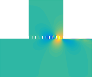
Figure 3. Iso-colour plots of (a)  $\text{Re}(p)$ and (b)
  $\text{Re}(v)$ for a plane wave incidence at the sound amplification frequency
  $\unicode[STIX]{x1D714}=0.2329$ (850 Hz) with an amplitude
  $|P(y)|=10^{-3}$. (c,d) Amplitude and phase of
  $v$ along the perforated plate at
  $y$ positions (red thin lines: slightly below the plate; black segmented lines: in the middle of the holes; blue thick lines: slightly above the plate) denoted by the dashed lines in (b). Note that the fields are plotted for part of the backing cavity, the same as in figures 4, 5, and 13. It should also be noted that the preliminary result in this figure has been presented at the 25th AIAA/CEAS Aeroacoustics Conference (Dai & Aurégan Reference Dai and Aurégan2019).
The fields of the pressure  $p$ and transverse velocity
  $v$ are shown in figure 3(a,b) at the peak sound amplification frequency. A spatially growing wave appears along the perforated plate. The amplitude and phase of
  $v$ approximately remain the same across the plate, as shown in figure 3(c,d), which is in agreement with the previous experiment where the phase variations on both sides of the perforated plate have been measured (Celik & Rockwell Reference Celik and Rockwell2004). It can also be found in figure 3(c) that the growth always happens in the small holes, suggesting that the large-scale spatially growing wave is linked to the small-scale KH instability of the shear flow over the holes. However, the hydrodynamic wavelength of interest is close to the length of the perforated plate
  $L$ (Sever & Rockwell Reference Sever and Rockwell2005) rather than the holes
  $L_{o}$, as shown by the fields and also by the phase in figure 3(d). This means that the backing cavity plays an important role in this phenomenon and it is difficult to explain the large-scale hydrodynamic wave and the related sound amplification by only examining the instability in the individual holes. Moreover, the long wavelength, compared with the period of perforation (for the present case
  $\unicode[STIX]{x1D706}_{hy}/(L_{o}+L_{s})\approx 10$), suggests that a homogenized description of the perforated plate can be used.
4 Global mode analysis
We perform a global mode analysis of the flow in the cavity segment and consider an analogy with flow oscillations in an open cavity. The goals are two-fold: (i) to explain the large-scale instability along the cavity-backed perforated plate; (ii) to better understand cavity flow oscillations. Since the purpose is not to describe every detail of the flow and acoustics, the classical and simple plate impedance model of Guess (Reference Guess1975) is used to describe the perforated plate with flow,  $Z_{p}=(R+R_{f})/\unicode[STIX]{x1D70E}+\text{i}\unicode[STIX]{x1D714}(T+\unicode[STIX]{x1D6FF})/\unicode[STIX]{x1D70E}$, where for a low sound pressure level
  $R_{f}=0.3(1-\unicode[STIX]{x1D70E}^{2})M_{0}$,
  $\unicode[STIX]{x1D6FF}=0.85L_{o}(1-0.7\sqrt{\unicode[STIX]{x1D70E}})(1+305M_{0}^{3})^{-1}$ and
  $\unicode[STIX]{x1D70E}$ is the open area ratio of the perforated plate
  $\unicode[STIX]{x1D70E}=L_{o}/(L_{o}+L_{s})$. However, it should be noted that such an impedance model can lead to inaccuracy in describing wave propagation in a flow duct, especially when the flow velocity is high (Dai & Aurégan Reference Dai and Aurégan2016; Aurégan Reference Aurégan2018). For this reason, only a qualitative comparison can be made between the discrete and homogenized models, and a quantitative agreement requires a more precise homogenization of a perforated plate with flow. To keep the gap small, a rather low flow speed is considered in this article (
 $M_{0}=0.1$). The flow and geometrical parameters are the same as § 3. The parameter
  $R$, which represents the system damping and in practice can be changed by covering the perforated plate with additional wiremesh sheets, is varied in the global mode analysis.
4.1 Unstable and stable global modes

Figure 4. Spatial distribution of a global mode: (a,b) unstable,  $\unicode[STIX]{x1D714}_{G}=2.2898\times 10^{-1}-1.0378\times 10^{-4}\text{i}$ (
 $835.78-0.3788\text{i}$ Hz), calculated with
  $R=0.0174$; (c,d) stable,
  $\unicode[STIX]{x1D714}_{G}=2.288\times 10^{-1}+1.1038\times 10^{-4}\text{i}$ (
 $835.12+0.40287\text{i}$ Hz), calculated with
  $R=0.0175$.
With an initial frequency,  $\unicode[STIX]{x1D714}_{0}$, the optimization procedure described in § 2.3 leads to the complex frequency of a global mode of the flow system,
  $\unicode[STIX]{x1D714}_{G}$. The corresponding eigenvector of
  $\unicode[STIX]{x1D648}_{fl}$ gives the coefficients of the transverse modes that assemble the global mode. Iso-colour plots of the real part of
  $p$ and
  $v$ of the global mode are presented in figure 4. As the damping parameter
  $R$ is varied, this mode can be either unstable as shown in figure 4(a,b) or stable as shown in figure 4(c,d). The spatial distributions of the global mode at the two states are visually identical, so one cannot distinguish unstable from stable regimes by seeing the disturbance fields.

Figure 5. Contour lines of  $\text{Re}(v)$ for a neutral global mode: (a) total, (b) hydrodynamic and (c) acoustic. The search for the neutral global mode, by adjusting
  $R$, stops when
  $|\text{Im}(\unicode[STIX]{x1D714}_{G})/\text{Re}(\unicode[STIX]{x1D714}_{G})|<10^{-10}$. In this figure,
  $\unicode[STIX]{x1D714}_{G}=2.289\times 10^{-1}-2.6921\times 10^{-12}\text{i}$ (
 $8.3546\times 10^{2}-9.8261\times 10^{-9}\text{i}$ Hz) results from
  $R\simeq 0.01745$.
In figure 5, the acoustic and hydrodynamic fields are separated. It is shown that the spatially growing wave observed in the total field is essentially the unstable hydrodynamic wave of the shear flow, although strong distortion occurs near the cavity downstream edge caused by evanescent acoustic waves.

Figure 6. Wavenumbers (a) and mode coefficients (b,c) of the normalized transverse modes in the cavity segment that assemble the neutral global mode in figure 5. Note that in (a), some neutral modes are slightly out of the real axis. This numerical issue can be mitigated by increasing the number of discrete points.

Figure 7. Amplitude (a,c) and phase (b,d) of  $v$ along the cavity opening for the neutral global mode in figure 5. Symbols: at the point just below
  $y=1$; lines: at the point just above
  $y=1$. Note that for each colour the symbols and the line overlap, since
  $v$ is continuous across
  $y=1$ and
  $\unicode[STIX]{x0394}h$ is small.
To more clearly see the structure of the global mode, the wavenumbers and coefficients of the transverse modes are presented in figure 6. Note that to avoid the complexity caused by a complex frequency, the neutral state shown in figure 5 is used in the discussion in figures 6 and 7. It is shown in figure 6(a) that the transverse modes in the cavity segment include acoustic modes propagating or decaying in the  $\pm x$ directions and hydrodynamic modes propagating, growing or decaying with the mean shear flow. The neutral hydrodynamic modes, resulting from the singularities of the Pridmore-Brown equation (Pridmore-Brown Reference Pridmore-Brown1958), describe the transport of vorticity in a shear flow and form a continuous spectrum on the real axis (Brambley et al. Reference Brambley, Darau and Rienstra2012). The unstable hydrodynamic mode is different from the unstable surface mode over a liner (Marx & Aurégan Reference Marx and Aurégan2013). The unstable surface mode is due to the coupling of a shear flow with a resonant lined wall and it only occurs over a very narrow frequency range near the resonance frequency of the liner (Aurégan & Leroux Reference Aurégan and Leroux2008; Marx et al. Reference Marx, Aurégan, Bailliet and Valière2010). The unstable hydrodynamic mode here merely arises from shear in the partly non-uniform mean flow (Kooijman, Hirschberg & Aurégan Reference Kooijman, Hirschberg and Aurégan2010; Dai & Aurégan Reference Dai and Aurégan2018). It happens over a wide frequency range, and the variation of its wavenumber with frequency is similar to that for a hyperbolic-tangent shear flow (Michalke Reference Michalke1965; Schmid & Henningson Reference Schmid and Henningson2000), as shown in figures 10(b) and 11(b). Therefore, it is called a KH-type instability, even though the flow is not the same as those for the well-known classical KH instability, that is, an infinitely thin shear layer or a hyperbolic-tangent shear flow. We also note that the previous experiment has suggested the analogous features between the instability along a slotted plate backed by a cavity and the classical KH instability over a cavity in the absence of the plate (Sever & Rockwell Reference Sever and Rockwell2005). This unstable mode can be differentiated from the acoustic modes decaying in the
  $-x$ direction by the Briggs–Bers causality criterion (Briggs Reference Briggs1964; Bers Reference Bers, Galeev and Sudan1983). Usually, the convectively unstable mode is accompanied with its complex conjugated counterpart, which decays in propagation. In the present case, the wavenumbers of the stable and unstable hydrodynamic modes are not complex conjugates owing to the plate impedance
  $Z_{p}$. The stable hydrodynamic mode can be distinguished from the acoustic modes decaying in the
  $+x$ direction by tracing it as
  $Z_{p}$ is varied from zero to the value used in the calculation of figure 6(a), or by seeing its modal profile of the transverse velocity which has a local peak around
  $y=1$.
The modal profiles of the transverse modes have been normalized so that  $|P(y)|_{max}=1$ before calculating the modal coefficients at the two ends of the cavity segment, as shown in figure 6(b,c). We can see that for the downstream-travelling modes, the amplitudes of the unstable and stable hydrodynamic modes and some less-attenuated acoustic modes are comparable at
  $x=0$ (generated by the scattering of the upstream-travelling acoustic modes). As they reach the downstream end,
  $x=L$, the unstable hydrodynamic mode dominates the others owing to its exponential growth in propagation. It scatters at the cavity downstream end, and acoustic modes travelling in the
  $-x$ direction are generated, of which some evanescent acoustic modes have amplitudes much higher than that of the least-attenuated acoustic mode. Although the least-attenuated acoustic mode has the highest amplitude at the destination
  $x=0$, meaning that it may be the most important upstream-travelling mode in closing the feedback loop, we will see that those high-amplitude evanescent modes generated at the downstream end are significant in affecting both the amplitude and phase of cavity flow disturbances.
As shown in figure 5, the strongest hydrodynamic and acoustic disturbances are both concentrated in the opening area of the cavity, that is, positions around  $y=1$. Thus, another way to analyse the global mode is to see the change of the disturbances along this line (
 $y=1$,
  $0\leqslant x\leqslant L$). The amplitude and phase of
  $v$ along the opening are plotted in figure 7(a,b), which denote the total effect of each group of transverse modes. For the hydrodynamic disturbances, the exponential growth in amplitude and the constant slope of the phase, except near the upstream end owing to the decaying hydrodynamic mode, reveal the dominant effect of the unstable hydrodynamic mode. For the acoustics, the high amplitude and the steeper phase variation near the downstream end indicate the considerable effect of the upstream-travelling evanescent modes generated at the downstream edge. The above observations of the disturbances along the cavity opening associated with different types of transverse modes agree with the analysis of mode coefficients in figure 6.
It is also noted in figure 7(a) that, owing to evanescent modes, the amplitude of the hydrodynamic part of  $v$ is significantly higher than the total
  $v$ near the downstream end of the cavity, which is qualitatively similar to the previous results of cavity flow oscillation where the fluctuating velocity
  $v$ associated with the KH instability was compared with the total
  $v$ calculated by the direct numerical simulation (DNS) (Rowley, Colonius & Basu Reference Rowley, Colonius and Basu2002).
Before examining the phase relation of the flow disturbances, we briefly review the mechanisms of oscillating cavity flows. Three physical mechanisms for the self-sustained oscillations in compressible cavity flows have been revealed. They are the acoustic feedback or the so-called Rossiter mode (Rossiter Reference Rossiter1964), the acoustic resonance in cavities (East Reference East1966; Tam Reference Tam1976; Koch Reference Koch2005) and the wake mode for long cavities (Rowley, Colonius & Basu Reference Rowley, Colonius and Basu2002). The interaction between the Rossiter mode and the acoustic resonance mechanism has been recently studied by Yamouni, Sipp & Jacquin (Reference Yamouni, Sipp and Jacquin2013). Since the present global mode frequency is much lower than the acoustic resonance frequencies of the cavity, the only relevant mechanism is the acoustic feedback: the spatially growing KH instability wave scatters into acoustic waves at the downstream edge, and the acoustic waves propagate upstream and excite the new instability wave. The idea of acoustic feedback can be found as early as of Lord Rayleigh (see Powell Reference Powell1995), and has been successfully used to understand edgetones (Powell Reference Powell1961). It was applied by Rossiter to explain the self-sustained cavity flow oscillations, and based on experimental data, a semi-empirical formula for oscillation frequencies was proposed, which is still widely used today. The Rossiter condition states that the travelling time of the instability wave and the feedback acoustic waves approximately equals an integral multiple of the time period of oscillation:  $L^{\ast }/U_{c}^{\ast }+L^{\ast }/c_{0}^{\ast }+\unicode[STIX]{x1D6FE}^{\ast }/f_{o}^{\ast }=j_{R}/f_{o}^{\ast }$, where
  $f_{o}^{\ast }$ is the oscillation frequency,
  $U_{c}^{\ast }$ is the convection velocity of the instability wave, the integer
  $j_{R}$ is the index of the Rossiter mode and
  $\unicode[STIX]{x1D6FE}^{\ast }$ is supposed to measure the time delay at the edges. However, the a posteriori Rossiter formula does not always give good predictions of oscillation frequencies when flow velocity or cavity geometry changes. To obtain a best fit to measured data, numerous emendations have been proposed (see Gloerfelt (Reference Gloerfelt2009) for a comprehensive dissection of those amended models).
Figure 7(c,d) presents  $v$ along the cavity opening, where the transverse modes are grouped into upstream- and downstream-travelling modes. The general growth and decay in amplitudes in the respective
  $\pm x$ directions are shown, and the growth approximately equals the decay. This is expected because the criterion in the present calculation of the global mode, that is, the associated eigenvalue of
  $\unicode[STIX]{x1D648}_{fl}$ equals unity, implies that the perturbations associated with the transverse modes travelling in the
  $+x$ (or
  $-x$) direction, after a feedback loop, still have the same amplitude. The criterion also requires that, after a feedback loop, the total phase change should be an integral multiple of
  $2\unicode[STIX]{x03C0}$. Figure 7(d) shows that the total phase change between the downstream- and upstream-propagating disturbances at
  $x=0$ is less than but close to
  $2\unicode[STIX]{x03C0}$, the difference can be explained by the phase lag in the scattering processes at the two ends. However, it is surprising to find that the phase change of the downstream-propagating disturbances at the two edges of the cavity is larger than
  $2\unicode[STIX]{x03C0}$. The downstream-propagating disturbances are mainly associated with the shear flow instability wave, and figure 7(c) does show that the phase difference of the unstable hydrodynamic mode at the two edges is larger than
  $2\unicode[STIX]{x03C0}$, that is, the hydrodynamic wavelength is smaller than the cavity length
  $\unicode[STIX]{x1D706}_{hy}<L$. The convection velocity and wavelength of the unstable hydrodynamic wave can also be quantitatively calculated from its wavenumber shown in figure 6(a),
  $k=8.585+5.246\text{i}$:
  $M_{c}/M_{0}=0.267$ and
  $\unicode[STIX]{x1D706}_{hy}/L=0.915$. This observation contrasts with the Rossiter condition that
  $\unicode[STIX]{x1D706}_{hy}$ is close to but slightly larger than
  $L$ for the present case. Nevertheless, we note in figure 7(d) that the phase of the upstream-travelling disturbances first has an apparent increase in the range
  $0.4<x<0.8$ owing to the evanescent acoustic modes and then shows a slight decrease related to the least-attenuated acoustic modes. In this way, the upstream-travelling evanescent waves reduce the total phase change around the feedback loop, so that the phase condition of the global mode can still be satisfied. It has been found that, compared with the Rossiter formula, incorporating a more complete description of acoustic waves inside the cavity (Tam & Block Reference Tam and Block1978; Yamouni, Sipp & Jacquin Reference Yamouni, Sipp and Jacquin2013) or taking into account the secondary feedback loops (Alvarez, Kerschen & Tumin Reference Alvarez, Kerschen and Tumin2004) leads to a more accurate prediction of oscillation frequencies in certain situations, whereas the present case particularly emphasizes the importance of those high-amplitude evanescent waves in the phase condition. The effect of evanescent waves might be another possible reason for that a universal empirical formula of oscillation frequencies has been found so difficult to obtain.
From figure 4, we know that as the system damping is varied, the same global mode can be either stable or unstable. Thus, seeing the change of  $\unicode[STIX]{x1D648}_{fl}$ with the parameter
  $R$ may provide further insights into the global instability of the flow system. As
  $R$ is increased,
  $\text{Im}(\unicode[STIX]{x1D714}_{G})$ indicates the transition of the global mode from unstable to stable regimes, as shown in figure 8(a). Note that
  $\text{Re}(\unicode[STIX]{x1D714}_{G})$ also slightly changes with
  $R$. In figure 8(b), the eigenvalues of
  $\unicode[STIX]{x1D648}_{fl}$ are shown where
  $R$ is changing but the frequency remains on the real axis, that is, the corresponding
  $\text{Re}(\unicode[STIX]{x1D714}_{G})$ is used as the frequency input in the calculations. In each case, the eigenvalues of
  $\unicode[STIX]{x1D648}_{fl}$ distribute in the following manner: one is located around 1, one around
  $0.15$–
 $0.11\text{i}$, and all the others are nearly 0 because
  $\unicode[STIX]{x1D648}_{fl}$ is close to singular. It is observed that as
  $R$ deviates from the value for the temporally neutral state whereas the frequency remains on the real axis, the eigenvalue in the shaded area deviates from unity. We adopt the loop gain concept (Powell Reference Powell1961; Rowley et al. Reference Rowley, Williams, Colonius, Murray and Macmynowski2006; Illingworth, Morgans & Rowley Reference Illingworth, Morgans and Rowley2012) and define the amplitude of this eigenvalue as the feedback-loop gain. It is shown in figure 8(c) that such a gain, being larger or smaller than 1, is the criterion for the global mode being unstable or stable. Figure 8(d) shows that increasing the parameter
  $R$ leads to a stabilization effect, that is, a reduction in the spatial growth rate of the unstable hydrodynamic mode. This might explain, from a homogeneous point of view, that in the previous investigations where the self-sustained oscillations occurred the cavity-backed perforated or slotted plates all had large open area ratios (around 65 %–90 %) (Celik & Rockwell Reference Celik and Rockwell2002, Reference Celik and Rockwell2004; Zoccola Reference Zoccola2004; Sever & Rockwell Reference Sever and Rockwell2005; Ekmekci & Rockwell Reference Ekmekci and Rockwell2007). Reducing the open area ratio leads to an increase of the equivalent resistance of the perforated plate, and consequently stabilizes the flow. In some previous cases, the first global mode (
 $\unicode[STIX]{x1D706}_{hy}\approx L$) has been found stable whereas some high-order global modes (
 $j\unicode[STIX]{x1D706}_{hy}\approx L$, where the mode index
  $j=2,3,\ldots ,j_{max}$) are unstable (Nakiboglu, Manders & Hirschberg Reference Nakiboglu, Manders and Hirschberg2012; Yamouni, Sipp & Jacquin Reference Yamouni, Sipp and Jacquin2013). These and the present results indicate that the convective hydrodynamic instability is a necessary but not a sufficient condition for such global instability, for that is decided by whether the loop gain is larger than unity. Note that in other flows such as wakes and hot jets (Martini, Cavalieri & Jordan Reference Martini, Cavalieri and Jordan2019), the mechanism of global instability can be provided by absolute instability (Huerre & Monkewitz Reference Huerre and Monkewitz1985).

Figure 8. (a) Variation of the complex frequency of the global mode as  $R$ is increased. (b–d) Variations of the eigenvalues of
  $\unicode[STIX]{x1D648}_{fl}$, the feedback-loop gain, and the wavenumbers of the transverse modes in the cavity segment, respectively, as
  $R$ is increased whereas the corresponding
  $\text{Re}(\unicode[STIX]{x1D714}_{G})$ is used as the frequency input in the calculations.
We end this subsection with a note on the difference between acoustic resonance and flow–acoustic resonance. Without flow, trapped modes in acoustics with real resonance frequencies that decay towards infinity and quasi-trapped modes with complex resonance frequencies owing to energy leak or damping, which makes the quasi-trapped modes temporally decaying, have been studied by Evans, Levitin & Vassiliev (Reference Evans, Levitin and Vassiliev1994), Koch (Reference Koch2005), Linton & McIver (Reference Linton and McIver2007), Duan et al. (Reference Duan, Koch, Linton and Mciver2007), Hein, Koch & Nannen (Reference Hein, Koch and Nannen2010), Pagneux (Reference Pagneux2013), Lyapina et al. (Reference Lyapina, Maksimov, Pilipchuk and Sadreev2015), Xiong, Bi & Aurégan (Reference Xiong, Bi and Aurégan2016) and others. The flow–acoustic resonance (or global mode) in the present study has both acoustic and hydrodynamic contributions. Determined by the balance of the energy transferred from the mean flow to the perturbations and the energy damped and radiated, the complex resonance frequency can have a negative, zero or positive imaginary part denoting a temporally unstable, neutral or stable mode, respectively.
4.2 Linear system response to external forcing

Figure 9. Reflection and transmission coefficients of a plane acoustic wave incident on the cavity segment from the upstream duct, calculated from (2.14). The six thick lines denote  $R$ decreasing from 0.019 to 0.018 with decrements of 0.0002, the five thin lines denotes
  $R$ from 0.0179 to 0.0175 with decrements of 0.0001. In the enlarged view of the sound blocking, four more lines are inserted between the lines of
  $R=0.018$ and 0.0179. Note that the global mode is stable for all these values of
  $R$.
$R$.
The unstable global modes and the consequent self-sustained oscillations of cavity flows have been the focus of much research, as reviewed by Rockwell & Naudascher (Reference Rockwell and Naudascher1978), Rowley & Williams (Reference Rowley and Williams2006) and Gloerfelt (Reference Gloerfelt2009), whereas the temporally decaying flow–acoustic resonances have received little attention. In this subsection, we explore the stable global mode by seeing the system response to external forcing, such as acoustic and vortical waves. Small perturbations in an unstable system grow in time until nonlinear saturation, which limits the amplitudes of self-sustained oscillations. For a stable system, however, it is believed that a linear model can predict the system response if the forcing amplitude is sufficiently small (Rowley et al. Reference Rowley, Williams, Colonius, Murray and Macmynowski2006; Illingworth, Morgans & Rowley Reference Illingworth, Morgans and Rowley2012).
Reflection and transmission coefficients of a plane wave incident on the cavity segment from the upstream duct are presented in figure 9. The parameter  $R$ is varied over a range so that the complex frequency of the stable global mode,
  $\unicode[STIX]{x1D714}_{G}$, progressively approaches the real axis but does not reach it (
 $\text{Im}(\unicode[STIX]{x1D714}_{G})>0$). As
  $\text{Im}(\unicode[STIX]{x1D714}_{G})$ reduces, resulting from the decreasing
  $R$, it is shown that at first the global mode behaves in the manner of quasi-trapped modes in acoustics without flow:
  $|R^{+}|$ increases and approaches unity, whereas
  $|T^{+}|$ decreases and approaches zero (Xiong, Bi & Aurégan Reference Xiong, Bi and Aurégan2016). The enlarged view shows that
  $|T^{+}|$ has a minimum around 0.014, and this value can be further reduced by adjusting
  $R$. As
  $\text{Im}(\unicode[STIX]{x1D714}_{G})$ continues to reduce, however,
  $|R^{+}|$ can be larger than 1, which is the limit in no-flow cases, and sound blocking turns into sound amplification. It should be noted that when
  $\text{Im}(\unicode[STIX]{x1D714}_{G})$ is very close to zero, the shear layer thickening owing to high-amplitude oscillations might lead to a saturation effect (Boujo, Bauerheim & Noiray Reference Boujo, Bauerheim and Noiray2018).

Figure 10. Decomposition of the plane-wave transmission from the upstream to the downstream ducts as the frequency sweeps from 0.1918 (700 Hz) to 0.274 (1000 Hz). In the calculation,  $R=0.0175$, which leads to
  $\unicode[STIX]{x1D714}_{G}=2.288\times 10^{-1}+1.1038\times 10^{-4}\text{i}$ (
 $835.12+0.40287\text{i}$ Hz). (a) Transmission coefficients at
  $x=0$, (b) propagation of the downstream-travelling modes in the cavity segment, (c) transmission coefficients at
  $x=L$. In (a–c), the downstream-travelling modes in the cavity segment are sorted as follows: the first to the
  $N_{2p}$th modes are acoustic modes sorted according to their wavenumbers; the
  $N_{2p}+1$th to the
  $N_{2p}+N_{1}$th modes are hydrodynamic modes, of which the
  $N_{2p}+1$th mode is unstable and the
  $N_{2p}+2$th mode is stable. (d) Transmission coefficients: squares denote the result from (2.14), crosses denote the result from (4.1), the triangles and inverted triangles represent hydrodynamic and acoustic contributions in (4.1), respectively. The vertical dashed line in (d) denotes the real part of
  $\unicode[STIX]{x1D714}_{G}$.
The transmission process between the plane waves in the upstream and downstream ducts can be divided into three steps. First, the plane wave from the upstream duct excites the downstream-travelling modes in the cavity segment, denoted by a row vector  $\boldsymbol{T}_{1}$ with
  $N_{2p}+N_{1}$ elements being the coefficients of the excited modes at the upstream end. The second step is the propagation of those modes from the upstream to the downstream ends of the cavity segment, denoted by a
  $(N_{2p}+N_{1})\times (N_{2p}+N_{1})$ diagonal matrix
  $\unicode[STIX]{x1D64B}_{d}$ with on the diagonal the values of
  $\exp (-\text{i}k_{n}L)$, where
  $k_{n}$ is the wavenumber of the
  $n\text{th}$ downstream-travelling mode. The third step accounts for the scattering at the downstream end, denoted by a column vector
  $\boldsymbol{T}_{2}$ with
  $N_{2p}+N_{1}$ elements being the transmission coefficients of the downstream-travelling modes in the cavity segment to the plane wave in the downstream duct.
  $\boldsymbol{T}_{2}$ can be obtained from matching the modes at the downstream end of the cavity segment, since the downstream-travelling modes in the cavity segment are the only incoming waves to this interface.
  $\boldsymbol{T}_{1}$ should be extracted from the scattering matrix of the whole cavity segment. Then, the plane-wave transmission from the upstream to the downstream ducts is formulated as,
 $$\begin{eqnarray}T^{+}=\boldsymbol{T}_{1}\unicode[STIX]{x1D64B}_{d}\boldsymbol{T}_{2}.\end{eqnarray}$$
Figure 11. Decomposition of the plane-wave transmission from the upstream to the downstream ducts. All parameters for calculation are the same as in figure 11, except  $R=0.0179$, which leads to
  $\unicode[STIX]{x1D714}_{G}=2.2808\times 10^{-1}+9.6396\times 10^{-4}\text{i}$ (
 $832.49+3.5184\text{i}$ Hz). The real part of
  $\unicode[STIX]{x1D714}_{G}$ is denoted by the vertical dashed line in (d). For the descriptions of the subfigures, see figure 10.
Comparison between the results from (4.1) and (2.14) is shown in figure 10(d), and the transmission decomposition is verified. The separate contributions to  $|T^{+}|$ from the downstream-travelling hydrodynamic and acoustic modes in the cavity segment are also presented. It is shown that the peak of total
  $|T^{+}|$ is lower than that related to the hydrodynamic modes, which can be understood as the result of the phase difference between the plane waves in the downstream duct scattered by the hydrodynamic and acoustic waves in the cavity segment. For each frequency, the amplitudes of the elements of
  $\boldsymbol{T}_{1}$,
  $\unicode[STIX]{x1D64B}_{d}$ and
  $\boldsymbol{T}_{2}$ are plotted in figure 10(a–c), respectively. From
  $P_{d}$ (elements on the diagonal of
  $\unicode[STIX]{x1D64B}_{d}$) in figure 10(b), we can see that the only amplified mode is the unstable hydrodynamic mode. The amplitude of
  $P_{d}$ for this mode first increases then decreases with the increasing frequency, with a peak at
  $\unicode[STIX]{x1D714}=0.2115$. Such a trend reflects the variation of the spatial growth rate with frequency, which is similar to that obtained from a hyperbolic-tangent shear flow (Michalke Reference Michalke1965; Tam & Block Reference Tam and Block1978). However, the frequency of the peak spatial growth rate is not the peak frequency of sound amplification, which means the resonance frequency is not determined by the spatial growth rate of the unstable hydrodynamic wave. In figure 10(c), it is shown that the scattering from the unstable hydrodynamic mode in the cavity segment into the plane acoustic wave in the downstream duct is rather inefficient and no clear dependence on frequency can be observed. Note that for the least-attenuated acoustic mode,
  $|T_{2}|\approx 1.3$, which is mainly decided by the cross-area ratio between the segments. Finally, we find the frequency selection in figure 10(a) where the unstable hydrodynamic mode and some acoustic modes are highly excited at the global mode frequency. The decomposition of the plane-wave transmission demonstrates the excitation of the global mode or flow–acoustic resonance, and also the link between the transmission peak and the resonance.

Figure 12. Effect of  $\text{Im}(\unicode[STIX]{x1D714}_{G})$ on
  $|T^{+}|$ contributed from the hydrodynamic and acoustic modes in the cavity segment, calculated from (4.1). The arrow denotes the decreasing
  $R$ (0.02, 0.019, 0.0185, 0.0179 and 0.0175), which leads to a positive and decreasing
  $\text{Im}(\unicode[STIX]{x1D714}_{G})$. The vertical lines denote the corresponding
  $\text{Re}(\unicode[STIX]{x1D714}_{G})$.
In figure 11, with  $R=0.0179$, the same analysis is carried out again as done in figure 10. For this case, figure 9 shows a sound blocking at the flow–acoustic resonance frequency. First, figure 11(b,c) is not much different from figure 10, except that the spatial growth rate of the unstable hydrodynamic mode is slightly reduced by the increase of
  $R$. In figure 11(a), the excited flow–acoustic resonance is still observed. Compared with figure 10(a), the quality factor of the resonance is lower, corresponding to a larger
  $\text{Im}(\unicode[STIX]{x1D714}_{G})$. It is shown in figure 11(d) that, near the resonance frequency,
  $|T^{+}|$ contributed from the downstream-travelling hydrodynamic and acoustic modes in the cavity segment are both larger than unity and the two lines cross. Thus, the sound blocking can be understood as the plane waves in the downstream duct, scattered by these two types of modes in the cavity segment, are nearly the same in amplitude but opposite in phase. Strictly speaking, the sound blocking results from the destructive interaction between the hydrodynamic and acoustic modes in the scattering at the downstream end.
Figure 12 shows that, at resonance,  $|T^{+}|$ associated with the hydrodynamic modes (
 $|T_{hy}^{+}|$) increases as the positive
  $\text{Im}(\unicode[STIX]{x1D714}_{G})$ decreases. The variation of the spatial growth rate of the unstable hydrodynamic mode, owing to the changes of
  $R$ and
  $\text{Re}(\unicode[STIX]{x1D714}_{G})$, contributes a small part to the increase of
  $|T_{hy}^{+}|$, whereas the more effective excitation of such mode at a less-damped resonance is the main cause of
  $|T_{hy}^{+}|$ increasing, which can be observed from figures 10(a) and 11(a). Thus, the highly excited hydrodynamic instability wave at a lightly damped flow–acoustic resonance, that is, a small and positive
  $\text{Im}(\unicode[STIX]{x1D714}_{G})$, renders the incident sound wave blocked or amplified.

Figure 13. Excitation of the stable global mode by a vortical wave: (a,b) incident vortical wave; (c,d) response of the flow system. In the calculation,  $R=0.0175$ and
  $\unicode[STIX]{x1D714}=0.2288$ (835.12 Hz), which is the real part of
  $\unicode[STIX]{x1D714}_{G}$. The vortical wave is introduced by giving an amplitude to the neutral hydrodynamic mode associated with the flow shear at
  $y=0.9683$ in the upstream duct so that
  $|P(y)|_{max}=10^{-3}$.
The excitation of the stable global mode by a vortical wave is demonstrated in figure 13. This suggests that, in practice, a stable cavity flow, excited by turbulent boundary-layer fluctuations, could produce sound that can be measured in the upstream and downstream ducts. Thus, it is possible that some of the previously observed cavity oscillations and sound emissions were produced by this mechanism, as discussed by Rowley et al. (Reference Rowley, Williams, Colonius, Murray and Macmynowski2006), rather than self-sustained oscillations. There are two senses of amplification associated with the global mode. One is the sound amplification, that is, the transmitted sound wave compared with the incident sound wave, which is an issue of noise control. The other is the ratio of the amplitudes of local fluctuations (near the cavity downstream edge in this case) to that of the incident acoustic or vortical disturbance. It is shown in figure 13 that the second amplification can be extremely large, which can potentially cause structural fatigue damage.
5 Conclusion
Flow–acoustic resonance in a cavity covered by a same-length perforated plate in a flow duct has been studied by a 2-D linear multimodal analysis. The mean shear flow in the duct was assumed unchanged in the streamwise direction and the acoustic and hydrodynamic disturbances were described by the LEEs with a resistive layer at the entrance of each hole in the plate. First, a hole-by-hole description of the flow–acoustic coupling shows a spatially growing wave along the perforated plate, with a wavelength close to the plate length but much larger than the period of perforation, which suggests that a homogenized approach can be used.
We then performed the travelling mode and global mode analyses of the flow where the perforated plate was represented by a homogeneous impedance. The global mode was constructed from the travelling hydrodynamic and acoustic waves by the feedback-loop closure principle. For the global mode, the agreement between the analyses of the travelling mode coefficients and the local fluctuations along the cavity opening has been shown. The spatially growing wave along the perforated plate is, from a homogeneous point of view, essentially a KH-type instability wave of shear flow, strongly distorted by evanescent acoustic waves near the downstream edge. The phase difference of the unstable hydrodynamic mode at the two edges has been found to be a bit larger than  $2\unicode[STIX]{x03C0}$ in this case, whereas the upstream-travelling evanescent waves reduce the total phase change around the feedback loop, so that the phase condition of the global mode can still be satisfied. These results indicate the significant effects of the high-amplitude evanescent waves near the downstream edge on both the amplitude and phase of cavity flow disturbances. Determined by the balance of the energy transferred from the mean flow to the perturbations and the energy damped and radiated, the complex resonance frequency can have a negative, zero or positive imaginary part, denoting a temporally unstable, neutral or stable mode, respectively. All three regimes of the global mode have been observed as the system damping is varied. The criterion of the global instability is discussed: the feedback-loop gain being larger or smaller than unity determines the global mode being unstable or stable.
The stable global mode is further studied by seeing the linear system response to external forcing. Owing to the highly excited hydrodynamic instability wave, both sound blocking and sound amplification at a lightly damped resonance are observed. It has also been shown that a stable cavity flow can produce sound when the flow–acoustic resonance is excited by a vortical wave.
Acknowledgements
This work has been supported by the National Natural Science Foundation of China no. 51876120. I am grateful to Y. Aurégan and V. Pagneux for the three-hour discussion in Le Mans in October 2018 and email communications that helped improve this article.


