


1 Introduction
The separation of a boundary layer from a surface can occur due to a sharp geometric edge or adverse pressure gradient (APG). The former category has been investigated extensively through classical configurations such as backward-facing step (e.g. Troutt, Scheelke & Norman Reference Troutt, Scheelke and Norman1984; Le, Moin & Kim Reference Le, Moin and Kim1997), which features a fixed separation front at the geometric edge. The APG-induced separation has an additional complexity due to its intermittent behavior; the separation and reattachment locations vary due to small changes in the pressure gradient (Simpson, Chew & Shivaprasad Reference Simpson, Chew and Shivaprasad1981). In APG-induced separation, a turbulent boundary layer (TBL) decelerates and thickens, and eventually departs from the surface with a large wall-normal velocity (Simpson Reference Simpson1989). The region immediately downstream from the separation is characterized by a ‘bubble’ of backward flow. In strong APG-induced separation, the height of the separation bubble is as thick as the preseparation shear layer, resulting in a significant blockage (Alving & Fernholz Reference Alving and Fernholz1996). The smaller bubble of a mild APG-induced separation is also important as it is frequently observed at the upper efficiency limit of aeronautical components such as wings, high-lift devices, turbine blades and diffusers (Ashjaee & Johnston Reference Ashjaee and Johnston1980). In these systems, flow separation causes loss of performance is terms of lift reduction and drag increase (Gad-el-Hak Reference Gad-el-Hak2000).
Flow separation in the symmetry plane of two-dimensional (2D) geometries has been considered as 2D separation in previous investigations. The main feature is that flow detachment and attachment lines are assumed to be rectilinear in the spanwise direction. However, such a 2D pattern is difficult to experimentally establish due to the lateral confinement present in any 2D set-up. Vortices at the corners of the cross-section affect the entire flow field (Malm, Schlatter & Henningson Reference Malm, Schlatter and Henningson2012). An example is the three-dimensional (3D) mean flow observed in the 2D symmetric diffuser of Ashjaee & Johnston (Reference Ashjaee and Johnston1980). The separated flow over a 2D airfoil also develops a 3D pattern, as observed in the visualizations of Moss & Murdin (Reference Moss and Murdin1968) and Broeren & Bragg (Reference Broeren and Bragg2001). The flow pattern typically consists of a saddle point at the symmetry plane with a curved separation line connecting to the corner vortices (Délery Reference Délery2013).
Previous investigations of 2D separation have applied passive correction techniques to reduce the effect of corner flows and interaction of the separated shear layer with other flow structures. For example, Simpson, Strickland & Barr (Reference Simpson, Strickland and Barr1977) and Simpson et al. (Reference Simpson, Chew and Shivaprasad1981) investigated a 2D turbulent separation bubble (TSB) over a flat plate, induced by the airfoil-type pressure gradient of a curved upper roof. An adjustable spanwise scoop was used at the leading edge of the roof to remove the boundary layer. Perry & Fairlie (Reference Perry and Fairlie1975) also investigated the TSB over a flat surface generated by a diverging–converging roof. A secondary false roof was applied to isolate the separated shear layer. Weiss, Mohammed-Taifour & Schwaab (Reference Weiss, Mohammed-Taifour and Schwaab2015) and Mohammed-Taifour & Weiss (Reference Mohammed-Taifour and Weiss2016) carried out detailed investigations of unsteadiness in a TSB generated by a diverging–converging roof equipped with a bleed slot. In a different method, Dianat & Castro (Reference Dianat and Castro1991) generated a TSB over a flat plate by applying suction from a spanwise porous cylinder mounted above the plate. Thompson & Whitelaw (Reference Thompson and Whitelaw1985) investigated TBL separation over a trailing-edge flap. They applied passive control vanes on the sidewalls to reduce the corner flows and placed several layers of screen on the pressure side of the flap to enforce a potential flow. In an attempt to avoid the 3D topology induced by the corner flows, Dengel & Fernholz (Reference Dengel and Fernholz1990) investigated separation on the axisymmetric boundary layer of a body of revolution. However, even over an axisymmetric body, the separation lines are not perfectly 2D and form a string of successive nodes and saddle points (Délery Reference Délery2013). These relatively complex set-ups were meant to generate 2D separation for simplification of analysis and evaluation of 2D computations.
In spite of the extensive investigation of 2D separation, separated flows are commonly 3D in industrial applications. Cherry, Elkins & Eaton (Reference Cherry, Elkins and Eaton2008) mentioned that all practical separated flows have a 3D topology, even in the mean velocity field. They specifically avoided any symmetry and characterized the mean flow field of two asymmetric 3D diffusers using magnetic resonance velocimetry. Their 3D diffuser consisted of top and side walls diverging at different angles. This experiment became a benchmark for the evaluation of numerical simulations by Ohlsson et al. (Reference Ohlsson, Schlatter, Fischer and Henningson2010) and Malm et al. (Reference Malm, Schlatter and Henningson2012). The numerical simulations of 3D flows is more challenging as the common turbulence closure models fail to correctly predict the flow statistics (Malm et al. Reference Malm, Schlatter and Henningson2012). In a more applied investigation, Duquesne, Maciel & Deschênes (Reference Duquesne, Maciel and Deschênes2015) investigated the unsteady structures of a 3D separated flow in the diffuser of a bulb turbine. To the best of the authors’ knowledge, 3D separated flows have rarely been investigated using modern flow diagnostics even though their turbulence structure and dynamics can be different from those with an enforced 2D flow.
Separated flows can be intermittent, unsteady and 3D. The intermittency of the separation region is characterized using
 $\unicode[STIX]{x1D6FE}$
, defined as the time fraction of forward flow (Simpson et al.
Reference Simpson, Strickland and Barr1977). The incipient detachment (ID), intermittent transitory detachment (ITD) and transitory detachment (TD) indicate locations where
$\unicode[STIX]{x1D6FE}$
, defined as the time fraction of forward flow (Simpson et al.
Reference Simpson, Strickland and Barr1977). The incipient detachment (ID), intermittent transitory detachment (ITD) and transitory detachment (TD) indicate locations where
 $\unicode[STIX]{x1D6FE}$
is 0.99, 0.8 and 0.5, respectively (Simpson Reference Simpson1996). However, flow reversal does not necessarily indicate separation in unsteady flows. Sears & Telionis (Reference Sears and Telionis1975) observed, based on evaluation of numerical and experimental data, that separation occurs in unsteady flows when wall shear vanishes and the local streamwise velocity is equal to the velocity of the moving separated structure. In 2D unsteady boundary layers, Haller (Reference Haller2004) defined separation based on formation of a spike in the material lines near the wall. Surana, Grunberg & Haller (Reference Surana, Grunberg and Haller2006) developed a mathematical theory for steady 3D flows using nonlinear dynamical systems. Their analysis showed that in steady flow only four surface signatures of separation are feasible: saddle-spiral, saddle-node, saddle-limit cycle and limit cycles. Surana et al. (Reference Surana, Jacobs, Grunberg and Haller2008) extended this analysis to unsteady 3D flows. However, experimental investigations are required to further extend the analysis and identify the coherent structures of separated turbulent flows.
$\unicode[STIX]{x1D6FE}$
is 0.99, 0.8 and 0.5, respectively (Simpson Reference Simpson1996). However, flow reversal does not necessarily indicate separation in unsteady flows. Sears & Telionis (Reference Sears and Telionis1975) observed, based on evaluation of numerical and experimental data, that separation occurs in unsteady flows when wall shear vanishes and the local streamwise velocity is equal to the velocity of the moving separated structure. In 2D unsteady boundary layers, Haller (Reference Haller2004) defined separation based on formation of a spike in the material lines near the wall. Surana, Grunberg & Haller (Reference Surana, Grunberg and Haller2006) developed a mathematical theory for steady 3D flows using nonlinear dynamical systems. Their analysis showed that in steady flow only four surface signatures of separation are feasible: saddle-spiral, saddle-node, saddle-limit cycle and limit cycles. Surana et al. (Reference Surana, Jacobs, Grunberg and Haller2008) extended this analysis to unsteady 3D flows. However, experimental investigations are required to further extend the analysis and identify the coherent structures of separated turbulent flows.
Several models have been proposed to describe the mean flow in 2D separation. Owing to the negligible wall shear stress at the separation region, the classical inner-layer scaling of wall flows does not hold. Using the local maximum of Reynolds shear stress, Perry & Schofield (Reference Perry and Schofield1973) proposed a velocity defect law for scaling the mean velocity profile upstream of the separation. Kline, Strawn & Bardina (Reference Kline, Strawn and Bardina1983) developed a single-variable correlation to model the velocity profile at the separated region based on a modified version of Coles’ law of the wall and law of the wake (Coles Reference Coles1956). Downstream of the separation, Simpson (Reference Simpson1996) described the mean backflow region with a three-layer model. The nearest layer to the wall is a viscous layer with negligible Reynolds shear stress while the outermost layer is a backflow region due to large-scale turbulent structures of the outer flow. In between these two layers, there is an overlap layer with a semi-logarithmic mean velocity profile. In the backflow region, Simpson (Reference Simpson1983) applied a scaling law based on the intensity and location of maximum backflow velocity. Agarwal & Simpson (Reference Agarwal and Simpson1990) showed that a velocity profile based on the law of the wall is not valid when the maximum backflow velocity is smaller than a quarter of the free-stream velocity. A general scaling of the velocity profile in the separation and backflow regions with small wall shear stress is still an open question (Skote & Henningson Reference Skote and Henningson2002).
The dominant direction of turbulent transport reverses from outward (away from the wall) in a zero pressure gradient boundary layer to an inward transport toward the wall in strong APG (Krogstad & Skåre Reference Krogstad and Skåre1995; Lee & Sung Reference Lee and Sung2008). The quadrant decomposition of Krogstad & Skåre (Reference Krogstad and Skåre1995) in a boundary layer with APG showed attenuation of ejection events and the appearance of motions in the first quadrant associated with the wall reflection of large-scale sweeps. The experiment of Song & Eaton (Reference Song and Eaton2002) demonstrated stronger sweep motions relative to ejections below the inflection point of the mean velocity profile in a separation bubble. Thompson & Whitelaw (Reference Thompson and Whitelaw1985) observed an increase of normal Reynolds stresses upstream and downstream of TSB due to the curvature of streamlines. Cuvier et al. (Reference Cuvier, Foucaut, Braud and Stanislas2014) observed two isolated regions of significant production of streamwise Reynolds stress in the beginning and the middle of the separation bubble due to flow deceleration and a flapping motion of large-scale structures, respectively. The direct numerical simulation (DNS) of Lee & Sung (Reference Lee and Sung2008) showed that APG increases the strength of the vortical structures of the outer layer, which results in an increase and the appearance of a second peak in the profile of the Reynolds shear stress.
The evolution of the classical coherent structures of a TBL as a result of APG and separation has most often investigated using numerical simulations due, for the most part, to the shortcomings of the available measurement systems at the time. The DNS of Marquillie, Laval & Dolganov (Reference Marquillie, Laval and Dolganov2008) showed that low-speed streaks of the TBL gradually disappear upstream of the separation. The streaks reappear along with new vortices downstream of the reattachment. The DNS of an attached TBL under APG by Lee & Sung (Reference Lee and Sung2009) also demonstrated weakening of low and high streaks and an increase of up to four times in their spanwise distance. Upon occurrence of the separation, strong negative and positive streamwise velocity fluctuations (
 ${\sim}$
25 % of mean velocity) populate the separation zone (Cuvier et al.
Reference Cuvier, Foucaut, Braud and Stanislas2014). These zones can be as long as
${\sim}$
25 % of mean velocity) populate the separation zone (Cuvier et al.
Reference Cuvier, Foucaut, Braud and Stanislas2014). These zones can be as long as
 $3\unicode[STIX]{x1D6FF}$
in the streamwise direction and
$3\unicode[STIX]{x1D6FF}$
in the streamwise direction and
 $0.5\unicode[STIX]{x1D6FF}$
in the spanwise direction, where
$0.5\unicode[STIX]{x1D6FF}$
in the spanwise direction, where
 $\unicode[STIX]{x1D6FF}$
is the boundary layer thickness close to the flow detachment (Cuvier et al.
Reference Cuvier, Foucaut, Braud and Stanislas2014). Lee & Sung (Reference Lee and Sung2009) showed evidence of quasi-streamwise and hairpin vortices using linear estimates of the conditional eddies around ejection motions. Although these investigations detail the evolution of coherent structures in 2D separation, their relevance to 3D separated flow is not clear. Characterization of coherent structures in 3D separated flows is required for the development of flow control strategies.
$\unicode[STIX]{x1D6FF}$
is the boundary layer thickness close to the flow detachment (Cuvier et al.
Reference Cuvier, Foucaut, Braud and Stanislas2014). Lee & Sung (Reference Lee and Sung2009) showed evidence of quasi-streamwise and hairpin vortices using linear estimates of the conditional eddies around ejection motions. Although these investigations detail the evolution of coherent structures in 2D separation, their relevance to 3D separated flow is not clear. Characterization of coherent structures in 3D separated flows is required for the development of flow control strategies.
The unsteadiness of a 2D separated flow has been associated with two dominant large-scale motions: (i) breathing motion; and (ii) shedding of spanwise vortices (Kiya & Sasaki Reference Kiya and Sasaki1983; Cherry, Hillier & Latour Reference Cherry, Hillier and Latour1984; Mohammed-Taifour & Weiss Reference Mohammed-Taifour and Weiss2016). These two motions are common in both geometry-induced and APG-induced separation. Proper orthogonal decomposition (POD) analysis of Mohammed-Taifour & Weiss (Reference Mohammed-Taifour and Weiss2016), based on planar particle image velocimetry (PIV) data over a larger field of view (FOV), showed that the first POD mode is associated with the breathing motion of the separation bubble and contains 30 % of the total turbulent kinetic energy. The breathing motion describes the contraction/expansion of the separation bubble, which is associated with a low-frequency wall-pressure fluctuation with a Strouhal number of
 $St\sim 0.01$
(Weiss et al.
Reference Weiss, Mohammed-Taifour and Schwaab2015). Mohammed-Taifour & Weiss (Reference Mohammed-Taifour and Weiss2016) reported about 90 % variation of the bubble size in their flow configuration as a result of this mode. Weiss et al. (Reference Weiss, Mohammed-Taifour and Schwaab2015) observed a medium St of about 0.35 due to the roll-up and shedding of vortices, which is in agreement with the DNS of Na & Moin (Reference Na and Moin1998). However, it is not clear whether the breathing and shedding modes play an important role in 3D separated flows.
$St\sim 0.01$
(Weiss et al.
Reference Weiss, Mohammed-Taifour and Schwaab2015). Mohammed-Taifour & Weiss (Reference Mohammed-Taifour and Weiss2016) reported about 90 % variation of the bubble size in their flow configuration as a result of this mode. Weiss et al. (Reference Weiss, Mohammed-Taifour and Schwaab2015) observed a medium St of about 0.35 due to the roll-up and shedding of vortices, which is in agreement with the DNS of Na & Moin (Reference Na and Moin1998). However, it is not clear whether the breathing and shedding modes play an important role in 3D separated flows.
Most of the investigations of 3D separated flows have been traditionally carried out using surface visualization techniques, such as oil streaks, to identify the topological characteristics using critical point theory (Werle Reference Werle1973). This theory is based on the surface pattern of skin-friction lines around critical points. A critical point is defined as a point with zero wall shear stress while the skin-friction lines are defined as trajectories on the surface that are tangent to the local skin-friction vector (Délery Reference Délery2001). The surface pattern surrounding the critical point can be of different types including saddle, focus and node points. In this theory, flow separation is identified when at least one saddle point (and the corresponding separation line) is present in the surface flow pattern of skin-friction lines (Délery Reference Délery2001). Duquesne et al. (Reference Duquesne, Maciel and Deschênes2015) carried out PIV in planes parallel to the walls of a bulb diffuser. They identified a saddle point on the diffuser side-wall by conditional averaging, while POD modes showed a series of foci and saddle points at the separation instants. Malm et al. (Reference Malm, Schlatter and Henningson2012) observed large-scale coherent structures with periodic motion at
 $St\sim 0.1$
(based on separation length) in the DNS of the 3D diffuser of Cherry et al. (Reference Cherry, Elkins and Eaton2008). They associated these structures with large streaks formed by sinusoidal oscillations within the diffuser. The previous surface visualizations and the limited number of modern flow measurements in 3D separation suggest that the dominant coherent structures are different from those of 2D separated flows.
$St\sim 0.1$
(based on separation length) in the DNS of the 3D diffuser of Cherry et al. (Reference Cherry, Elkins and Eaton2008). They associated these structures with large streaks formed by sinusoidal oscillations within the diffuser. The previous surface visualizations and the limited number of modern flow measurements in 3D separation suggest that the dominant coherent structures are different from those of 2D separated flows.
The objective of the current investigation is to characterize the coherent structures and separation mechanism of a 3D separated flow on the expanding wall of a diffuser. The diffuser has a rectangular cross-section and only one of the walls expands. The flow evolves into a 3D separated flow under the influence of the corner flows; no specific attempt is made to enforce a 2D separation. Measurements are carried out using planar PIV and tomographic PIV (tomo-PIV). A brief description of the experimental set-up, measurement systems and data reduction techniques are provided in § 2. The mean flow, Reynolds stresses and turbulent transport in the mid-span of the diffuser are characterized in § 3 for comparison with the literature on 2D separation. Flow instants with separation are investigated using conditional averaging of PIV and tomo-PIV in § 4. The analysis is further extended by characterization of the coherent structures using POD in § 5. The energetic POD modes are applied to develop a reduced-order model (ROM) of the separation mechanism in § 6.

Figure 1. (a) 3D schematic drawing of the set-up showing the flume and the modified test section. (b) Top view of the water flume holding a multi-segment plate. From left to right, the multi-segment plate consists of a curved leading edge (A–B), a long straight section with
 $3.4^{\circ }$
divergence (B–C), an arc (C–D) and a flat diffuser plate (D–E), followed by a straight section (E–F). The separation occurs on the diffuser plate where the
$3.4^{\circ }$
divergence (B–C), an arc (C–D) and a flat diffuser plate (D–E), followed by a straight section (E–F). The separation occurs on the diffuser plate where the
 $x$
–
$x$
–
 $y$
coordinate system is located. (c) A magnified view of the diffuser section. (d) Mean velocity,
$y$
coordinate system is located. (c) A magnified view of the diffuser section. (d) Mean velocity,
 $\langle U\rangle$
, and pressure coefficient,
$\langle U\rangle$
, and pressure coefficient,
 $C_{p}$
, are measured using a Pitot tube and plotted versus the streamwise axis (
$C_{p}$
, are measured using a Pitot tube and plotted versus the streamwise axis (
 $x^{\prime }$
) along the channel centreline. The error bars show standard deviation of the measurements.
$x^{\prime }$
) along the channel centreline. The error bars show standard deviation of the measurements.
2 Experimental procedure
A flow facility is built to form a relatively thick TBL over a flat plate. The TBL flows over a 2D diffuser where it separates from the expanding wall due to the APG present. Planar PIV is applied to characterize a large FOV around the separation location while the 3D motion of the separated flow in a smaller volume is scrutinized using tomo-PIV. The conditional sampling technique for detection of flow separation instants in 2D and 3D flows are explained in this section.
2.1 Flow set-up
A water flume with a rectangular cross-section has been modified to form a water tunnel by covering its free surface as shown in the schematic of figure 1(a). The acrylic plate on the top surface of the flume applies a no-slip boundary condition and prevents formation of surface waves. The flow passes through several honeycombs and screens before entering the channel to ensure a uniform flow. A 2D channel with variable cross-section is formed between the vertical sidewall of a water flume and a multi-segment wall with leading-edge (A–B), straight (B–C) and expanding (C–E) sections, as shown in figure 1(a) and the top view of figure 1(b). The dimensions of the set-up are indicated based on the expansion height of the diffuser,
 $H=165$
mm. The distance
$H=165$
mm. The distance
 $H$
is defined as the distance between points C and E, perpendicular to the flow direction, as seen in figure 1(b). The leading-edge section of A–B is an arc with a
$H$
is defined as the distance between points C and E, perpendicular to the flow direction, as seen in figure 1(b). The leading-edge section of A–B is an arc with a
 $3.63H$
(0.6 m) radius followed by a
$3.63H$
(0.6 m) radius followed by a
 $15.15H$
(2.5 m) long straight section (B–C) with a small diverging angle of
$15.15H$
(2.5 m) long straight section (B–C) with a small diverging angle of
 $3.4^{\circ }$
to develop a TBL at zero pressure gradient. The flow stays attached over this curve and the following flat plat as confirmed by tuft visualization. The boundary layer transition to turbulence is forced
$3.4^{\circ }$
to develop a TBL at zero pressure gradient. The flow stays attached over this curve and the following flat plat as confirmed by tuft visualization. The boundary layer transition to turbulence is forced
 $0.90H$
(150 mm) downstream of the start of the straight section (point B) using a 1.5 mm diameter wire. The distance between the side wall of the flume and the mid-point of section B–C is
$0.90H$
(150 mm) downstream of the start of the straight section (point B) using a 1.5 mm diameter wire. The distance between the side wall of the flume and the mid-point of section B–C is
 $1.52H$
(0.25 m). The depth of the channel (
$1.52H$
(0.25 m). The depth of the channel (
 $W$
) in the out-of-plane direction of figure 1 is about
$W$
) in the out-of-plane direction of figure 1 is about
 $3.03H$
(0.5 m). The C–D section is an arc with
$3.03H$
(0.5 m). The C–D section is an arc with
 $3.64H$
(0.6 m) radius connecting to the straight section of the diffuser (D–E), which is a flat plate with
$3.64H$
(0.6 m) radius connecting to the straight section of the diffuser (D–E), which is a flat plate with
 $3.03H$
(0.5 m) length and
$3.03H$
(0.5 m) length and
 $18.4^{\circ }$
angle with respect to the channel wall. The pressure-induced separation is formed
$18.4^{\circ }$
angle with respect to the channel wall. The pressure-induced separation is formed
 $2H$
(0.33 m) downstream of the start of the diffuser section as indicted in the magnified view of figure 1(c).
$2H$
(0.33 m) downstream of the start of the diffuser section as indicted in the magnified view of figure 1(c).
The
 $x$
–
$x$
–
 $y$
coordinate system is defined with respect to the diffuser plate as indicated in figure 1(b,c). The
$y$
coordinate system is defined with respect to the diffuser plate as indicated in figure 1(b,c). The
 $x$
-axis is aligned with the D–E section. The origin of the
$x$
-axis is aligned with the D–E section. The origin of the
 $x$
–
$x$
–
 $y$
coordinate system is placed at the point where
$y$
coordinate system is placed at the point where
 $\unicode[STIX]{x2202}\langle U\rangle /\unicode[STIX]{x2202}y=0$
at the wall. This origin merely serves as a reference for the coordinate system. The flow is intermittent and the instantaneous location of separation moves along the diffuser plate. The expansion height of the diffuser,
$\unicode[STIX]{x2202}\langle U\rangle /\unicode[STIX]{x2202}y=0$
at the wall. This origin merely serves as a reference for the coordinate system. The flow is intermittent and the instantaneous location of separation moves along the diffuser plate. The expansion height of the diffuser,
 $H$
, is used to normalize the coordinates as
$H$
, is used to normalize the coordinates as
 $X=x/H$
,
$X=x/H$
,
 $Y=y/H$
. Another straight section (E–F) is added downstream of the diffuser to prevent interaction of the separated shear layer with the wake. During set-up, tuft visualizations are applied to ensure an attached flow on the expanding arc (section C–D) and also on the wall of the water flume.
$Y=y/H$
. Another straight section (E–F) is added downstream of the diffuser to prevent interaction of the separated shear layer with the wake. During set-up, tuft visualizations are applied to ensure an attached flow on the expanding arc (section C–D) and also on the wall of the water flume.
The Re number based on the length of section B–C and the centreline velocity is about
 $8.1\times 10^{5}$
. A relatively thick TBL with a
$8.1\times 10^{5}$
. A relatively thick TBL with a
 $\unicode[STIX]{x1D6FF}$
thickness of approximately 52 mm forms just before the start of the diffuser curve. The
$\unicode[STIX]{x1D6FF}$
thickness of approximately 52 mm forms just before the start of the diffuser curve. The
 $\unicode[STIX]{x1D6FF}$
is estimated based on Schlichting (Reference Schlichting1979) following
$\unicode[STIX]{x1D6FF}$
is estimated based on Schlichting (Reference Schlichting1979) following
 $$\begin{eqnarray}\displaystyle \unicode[STIX]{x1D6FF}=0.37lRe_{l}^{-1/5}, & & \displaystyle\end{eqnarray}$$
where
 $l$
is the distance from the tripping wire to point C, and
$l$
is the distance from the tripping wire to point C, and
 $Re_{l}$
is based on the velocity at the centre of the channel (
$Re_{l}$
is based on the velocity at the centre of the channel (
 $U_{ref}$
) and
$U_{ref}$
) and
 $l$
. The ratio of the depth of the channel to the boundary layer thickness (
$l$
. The ratio of the depth of the channel to the boundary layer thickness (
 $W/\unicode[STIX]{x1D6FF}$
) is 9.6. However, the thickness of TBL rapidly increases in the expanding section due to the APG. Pitot tube measurements are taken to characterize the velocity and pressure along the centreline of the channel as indicated by
$W/\unicode[STIX]{x1D6FF}$
) is 9.6. However, the thickness of TBL rapidly increases in the expanding section due to the APG. Pitot tube measurements are taken to characterize the velocity and pressure along the centreline of the channel as indicated by
 $x^{\prime }$
axis in figure 1(b). The origin of
$x^{\prime }$
axis in figure 1(b). The origin of
 $x^{\prime }$
axis is aligned in the streamwise location with
$x^{\prime }$
axis is aligned in the streamwise location with
 $x=0$
as seen in figure 1(c). The velocity upstream of the diffuser at the centreline of the channel is
$x=0$
as seen in figure 1(c). The velocity upstream of the diffuser at the centreline of the channel is
 $0.45~\text{m}~\text{s}^{-1}$
, and gradually decreases in the diffuser as shown in figure 1(d). The pressure measurement in figure 1(d) also shows a relatively constant pressure coefficient at
$0.45~\text{m}~\text{s}^{-1}$
, and gradually decreases in the diffuser as shown in figure 1(d). The pressure measurement in figure 1(d) also shows a relatively constant pressure coefficient at
 $x^{\prime }<3H$
followed by an increase of the pressure coefficient in the diffuser section. The pressure coefficient is defined as
$x^{\prime }<3H$
followed by an increase of the pressure coefficient in the diffuser section. The pressure coefficient is defined as
 $C_{p}=(p-p_{c})/(0.5\times \unicode[STIX]{x1D70C}\times U_{ref}^{2})$
, where
$C_{p}=(p-p_{c})/(0.5\times \unicode[STIX]{x1D70C}\times U_{ref}^{2})$
, where
 $p_{c}$
and
$p_{c}$
and
 $U_{ref}=0.45~\text{m}~\text{s}^{-1}$
are the static pressure and velocity at
$U_{ref}=0.45~\text{m}~\text{s}^{-1}$
are the static pressure and velocity at
 $x^{\prime }=-10H$
, respectively. The inner scaling of the TBL at point C (just before the start of the diffuser curve) can be obtained from an estimation of the wall shear stress following
$x^{\prime }=-10H$
, respectively. The inner scaling of the TBL at point C (just before the start of the diffuser curve) can be obtained from an estimation of the wall shear stress following
 $$\begin{eqnarray}\displaystyle \unicode[STIX]{x1D70F}=0.0296\unicode[STIX]{x1D70C}U_{ref}^{2}Re_{l}^{-1/5}, & & \displaystyle\end{eqnarray}$$
where
 $\unicode[STIX]{x1D70C}$
is density of water (Schlichting Reference Schlichting1979). The estimated friction velocity and wall unit are
$\unicode[STIX]{x1D70C}$
is density of water (Schlichting Reference Schlichting1979). The estimated friction velocity and wall unit are
 $u_{\unicode[STIX]{x1D70F}}=0.0193~\text{m}~\text{s}^{-1}$
and
$u_{\unicode[STIX]{x1D70F}}=0.0193~\text{m}~\text{s}^{-1}$
and
 $\unicode[STIX]{x1D706}=52~\unicode[STIX]{x03BC}\text{m}$
, respectively.
$\unicode[STIX]{x1D706}=52~\unicode[STIX]{x03BC}\text{m}$
, respectively.

Figure 2. A schematic view of the planar and tomo-PIV set-ups. (a) The planar PIV set-up consists of four cameras in staggered configuration imaging the FOV through front surface mirrors. (b) The tomo-PIV set-up includes a combination of cylindrical and spherical optics to form a collimated laser sheet. The four cameras are arranged in a cross configuration. Cameras 2 and 4 have the largest solid angle (
 ${\sim}$
35) and image through a water-filled prism mounted on the wall of the channel (not shown here for clarity).
${\sim}$
35) and image through a water-filled prism mounted on the wall of the channel (not shown here for clarity).
2.2 Planar PIV
The separated flow is characterized using four PIV cameras, which simultaneously capture the velocity field upstream and downstream of the detachment locations in the mid-span of the plate. The combined FOV of the four CCD cameras covers
 ${\sim}1.45H$
(240 mm) in the streamwise direction (
${\sim}1.45H$
(240 mm) in the streamwise direction (
 $x$
) and
$x$
) and
 ${\sim}0.4H$
(66 mm) in the wall-normal direction (
${\sim}0.4H$
(66 mm) in the wall-normal direction (
 $y$
) as shown in figure 2(a). Each PIV camera (Imager ProX, LaVision GmbH) has a
$y$
) as shown in figure 2(a). Each PIV camera (Imager ProX, LaVision GmbH) has a
 $2048\times 2048$
pixels sensor with a pixel size of
$2048\times 2048$
pixels sensor with a pixel size of
 $7.4~\unicode[STIX]{x03BC}\text{m}\times 7.4~\unicode[STIX]{x03BC}\text{m}$
and a 14-bit resolution. The FOV of each camera is
$7.4~\unicode[STIX]{x03BC}\text{m}\times 7.4~\unicode[STIX]{x03BC}\text{m}$
and a 14-bit resolution. The FOV of each camera is
 ${\sim}75~\text{mm}\times 75~\text{mm}$
with a digital resolution of about
${\sim}75~\text{mm}\times 75~\text{mm}$
with a digital resolution of about
 $27~\text{pixels}~\text{mm}^{-1}$
, which varies slightly from one camera to another. Each camera is equipped with an SLR lens with a focal length of
$27~\text{pixels}~\text{mm}^{-1}$
, which varies slightly from one camera to another. Each camera is equipped with an SLR lens with a focal length of
 $f=105$
mm at an aperture setting of
$f=105$
mm at an aperture setting of
 $f/11$
. The estimated depth of field is
$f/11$
. The estimated depth of field is
 ${\sim}$
12 mm. The four PIV cameras are arranged in a staggered configuration and image through four front surface mirrors oriented at
${\sim}$
12 mm. The four PIV cameras are arranged in a staggered configuration and image through four front surface mirrors oriented at
 $45^{\circ }$
angle with respect to the line of sight of the cameras as shown in figure 2(a). This configuration allows the FOV of the side-by-side cameras at a magnification of 0.2 to overlap and form a continuous FOV. A calibration process using a 2D target is applied to correct for any optical and perspective distortion of the images, and later stitch the vector fields.
$45^{\circ }$
angle with respect to the line of sight of the cameras as shown in figure 2(a). This configuration allows the FOV of the side-by-side cameras at a magnification of 0.2 to overlap and form a continuous FOV. A calibration process using a 2D target is applied to correct for any optical and perspective distortion of the images, and later stitch the vector fields.
The FOV is illuminated by a Nd:YAG laser (Spectra-Physics, PIV400) with a maximum output power of
 $400~\text{mJ}~\text{pulse}^{-1}$
at 532 nm wavelength. A combination of spherical and cylindrical lenses generate a laser sheet with
$400~\text{mJ}~\text{pulse}^{-1}$
at 532 nm wavelength. A combination of spherical and cylindrical lenses generate a laser sheet with
 ${\sim}$
1 mm thickness and 300 mm width. The laser sheet and FOV are located
${\sim}$
1 mm thickness and 300 mm width. The laser sheet and FOV are located
 $1.5H$
above the bottom wall of the flume at the middle of the plate. The flume is seeded with
$1.5H$
above the bottom wall of the flume at the middle of the plate. The flume is seeded with
 $d_{p}=2~\unicode[STIX]{x03BC}\text{m}$
silver-coated spherical glass particles (SG02S40, Potters Industries) with a relative density of
$d_{p}=2~\unicode[STIX]{x03BC}\text{m}$
silver-coated spherical glass particles (SG02S40, Potters Industries) with a relative density of
 $\unicode[STIX]{x1D70C}_{p}=2.6~\text{g}~\text{cm}^{-3}$
. The response time of the tracers (
$\unicode[STIX]{x1D70C}_{p}=2.6~\text{g}~\text{cm}^{-3}$
. The response time of the tracers (
 $\unicode[STIX]{x1D70F}_{p}=\unicode[STIX]{x1D70C}_{p}d_{p}^{2}/18\unicode[STIX]{x1D707}$
,
$\unicode[STIX]{x1D70F}_{p}=\unicode[STIX]{x1D70C}_{p}d_{p}^{2}/18\unicode[STIX]{x1D707}$
,
 $\unicode[STIX]{x1D707}$
in the dynamic viscosity of the water) with respect to the inner time scale of the TBL (
$\unicode[STIX]{x1D707}$
in the dynamic viscosity of the water) with respect to the inner time scale of the TBL (
 $\unicode[STIX]{x1D70F}_{f}$
) is characterized using the Stokes number (Stk) of the tracers,
$\unicode[STIX]{x1D70F}_{f}$
) is characterized using the Stokes number (Stk) of the tracers,
 $Stk=\unicode[STIX]{x1D70F}_{p}/\unicode[STIX]{x1D70F}_{f}$
. The inner time scale of the flow is estimated from the wall-shear stress obtained using (2.2). The estimated Stk is
$Stk=\unicode[STIX]{x1D70F}_{p}/\unicode[STIX]{x1D70F}_{f}$
. The inner time scale of the flow is estimated from the wall-shear stress obtained using (2.2). The estimated Stk is
 ${\sim}2\times 10^{-4}$
, which indicates that the tracers follow the smallest eddies of the flow (i.e.
${\sim}2\times 10^{-4}$
, which indicates that the tracers follow the smallest eddies of the flow (i.e.
 $Stk\ll 1$
). Similar tracers have previously been used for detailed measurement of the inner layer at high-Reynolds turbulent channel flows using digital holographic microscopy by Talapatra & Katz (Reference Talapatra and Katz2012) and Ling et al. (Reference Ling, Srinivasan, Golovin, McKinley, Tuteja and Katz2016). The cameras and the laser system are synchronized using a programmable timing unit (PTU9, LaVision GmbH). The separation time between the two laser pulses is 2 ms and data acquisition is performed at 2 Hz. An ensemble of 7000 double-frame images is captured using each camera to ensure statistical convergence.
$Stk\ll 1$
). Similar tracers have previously been used for detailed measurement of the inner layer at high-Reynolds turbulent channel flows using digital holographic microscopy by Talapatra & Katz (Reference Talapatra and Katz2012) and Ling et al. (Reference Ling, Srinivasan, Golovin, McKinley, Tuteja and Katz2016). The cameras and the laser system are synchronized using a programmable timing unit (PTU9, LaVision GmbH). The separation time between the two laser pulses is 2 ms and data acquisition is performed at 2 Hz. An ensemble of 7000 double-frame images is captured using each camera to ensure statistical convergence.
To improve the signal-to-noise ratio (SNR) in the near-wall region, the minimum intensity of the ensemble of images is subtracted from each image. The images are then normalized by their ensemble average. The double-frame images are cross-correlated with a commercial software (DaVis 8.3, LaVision GmbH) using a multi-pass algorithm with a final window size of
 $32\times 32$
pixels (
$32\times 32$
pixels (
 $1.18\times 1.18~\text{mm}^{2}$
) and 75 % overlap. This results in a spatial dynamic range of
$1.18\times 1.18~\text{mm}^{2}$
) and 75 % overlap. This results in a spatial dynamic range of
 ${\sim}$
100 in the streamwise direction. The first valid vector from the wall is located at
${\sim}$
100 in the streamwise direction. The first valid vector from the wall is located at
 $Y=0.002$
. The universal outlier detection method of Westerweel & Scarano (Reference Westerweel and Scarano2005) is applied to detect the spurious vectors. Less than 2 % of the vectors are detected as outliers and replaced through linear interpolation. A summary of the specifications of the PIV system is provided in table 1. The uncertainty of the PIV system is estimated in Davis 8.4 (LaVision GmbH) using the method of Wieneke (Reference Wieneke2015) from statistical properties of the correlation peak. This method is based on the intensity difference of the first image frame and the second frame dewarped back using the computed displacement field. Inspection of the uncertainty fields shows that maximum local uncertainty within the FOV of all four cameras is
$Y=0.002$
. The universal outlier detection method of Westerweel & Scarano (Reference Westerweel and Scarano2005) is applied to detect the spurious vectors. Less than 2 % of the vectors are detected as outliers and replaced through linear interpolation. A summary of the specifications of the PIV system is provided in table 1. The uncertainty of the PIV system is estimated in Davis 8.4 (LaVision GmbH) using the method of Wieneke (Reference Wieneke2015) from statistical properties of the correlation peak. This method is based on the intensity difference of the first image frame and the second frame dewarped back using the computed displacement field. Inspection of the uncertainty fields shows that maximum local uncertainty within the FOV of all four cameras is
 ${\sim}0.008~\text{m}~\text{s}^{-1}$
(0.4 pixels), which is about 1.7 % of
${\sim}0.008~\text{m}~\text{s}^{-1}$
(0.4 pixels), which is about 1.7 % of
 $U_{ref}$
.
$U_{ref}$
.
Table 1. Imaging and processing parameters of the planar PIV and tomo-PIV experiments.

The initial stitching process of the four simultaneously acquired vector fields is carried out using the mapping function obtained from the 2D calibration target. An additional rotational and translational correction is applied using a custom function in MATLAB (MathWorks Inc.) based on cross-correlation of the velocity in the overlapped region of neighbouring cameras. An uncertainty analysis over the ensemble of the vectors shows that the maximum difference between the velocity magnitudes in the overlap region of any two cameras is
 ${\sim}6\times 10^{-3}~\text{m}~\text{s}^{-1}$
(0.3 pixels). A sample stitched instantaneous vector field from planar PIV is shown in figure 3(a). As is observed, there is no visible boundary between the vector fields of the four cameras. The vector field shows an upstream forward flow up to about
${\sim}6\times 10^{-3}~\text{m}~\text{s}^{-1}$
(0.3 pixels). A sample stitched instantaneous vector field from planar PIV is shown in figure 3(a). As is observed, there is no visible boundary between the vector fields of the four cameras. The vector field shows an upstream forward flow up to about
 $X=-0.3$
, where a large backflow region is identified with the contour enclosed by the solid line. There are also smaller backflow regions at about
$X=-0.3$
, where a large backflow region is identified with the contour enclosed by the solid line. There are also smaller backflow regions at about
 $X=-0.8$
and
$X=-0.8$
and
 $X=+0.1$
.
$X=+0.1$
.

Figure 3. (a) An instantaneous flow field captured using the four-camera planar PIV. The contours of the backflow region are enclosed by a solid line. The thick solid contour line shows the boundaries of the backflow region based on
 $\langle U\rangle =0$
. (b) Profiles of instantaneous velocity (
$\langle U\rangle =0$
. (b) Profiles of instantaneous velocity (
 $U$
) and the low-pass filtered velocity (
$U$
) and the low-pass filtered velocity (
 $U_{f}$
) are shown along
$U_{f}$
) are shown along
 $Y=0.025$
. The filtered signal (
$Y=0.025$
. The filtered signal (
 $U_{f}$
) only retains the large backflow region between
$U_{f}$
) only retains the large backflow region between
 $X=-0.25$
and
$X=-0.25$
and
 $-0.07$
. The
$-0.07$
. The
 $X=-0.25$
and
$X=-0.25$
and
 $X=-0.07$
points are separation and attachment locations, respectively.
$X=-0.07$
points are separation and attachment locations, respectively.
2.3 Tomo-PIV
The 3D characterization of the flow field in the separation zone is carried out using a tomo-PIV system (Elsinga et al.
Reference Elsinga, Scarano, Wieneke and van Oudheusden2006). The laser light from the same Nd:YAG laser as used for the planar PIV was shaped into a collimated laser sheet with 12 mm thickness and 100 mm width using a combination of spherical and cylindrical optics. The laser sheet was directed parallel to the diffuser surface from the bottom of the channel using a large, high-power mirror, as shown in figure 2(b). The laser sheet is carefully directed flush to the surface to minimize wall reflection, covering up to the wall-normal location of
 $y=12$
mm. Knife-edge filters are installed on the bottom glass wall of the channel to crop the low-energy tails of the sheet and provide a relatively top-hat intensity profile.
$y=12$
mm. Knife-edge filters are installed on the bottom glass wall of the channel to crop the low-energy tails of the sheet and provide a relatively top-hat intensity profile.
The same cameras as used for the planar PIV, equipped with the same
 $f=105$
mm SLR lens with the addition of Scheimpflug adapters, are arranged in a cross-like orientation as shown in figure 2(b). Cameras 2 and 4 have larger viewing angles and image through water-filled prisms installed on the vertical glass wall of the flume to reduce image distortion and astigmatism of particle images. The aperture of the SLR lens on camera 3 is set at
$f=105$
mm SLR lens with the addition of Scheimpflug adapters, are arranged in a cross-like orientation as shown in figure 2(b). Cameras 2 and 4 have larger viewing angles and image through water-filled prisms installed on the vertical glass wall of the flume to reduce image distortion and astigmatism of particle images. The aperture of the SLR lens on camera 3 is set at
 $f/16$
to collect more light from its backward scattering configuration, while the three other cameras image the FOV at an aperture setting of
$f/16$
to collect more light from its backward scattering configuration, while the three other cameras image the FOV at an aperture setting of
 $f/22$
. The depth of field of camera 3 with the smallest aperture of
$f/22$
. The depth of field of camera 3 with the smallest aperture of
 $f/16$
is
$f/16$
is
 ${\sim}$
23 mm, which covers the entire thickness of the laser sheet. The digital resolution of the 3D imaging system is
${\sim}$
23 mm, which covers the entire thickness of the laser sheet. The digital resolution of the 3D imaging system is
 $27.3~\text{voxels}~\text{mm}^{-1}$
with a measurement volume of
$27.3~\text{voxels}~\text{mm}^{-1}$
with a measurement volume of
 $(\unicode[STIX]{x0394}x,\unicode[STIX]{x0394}y,\unicode[STIX]{x0394}z)=75~\text{mm}\times 12~\text{mm}\times 70~\text{mm}$
, where
$(\unicode[STIX]{x0394}x,\unicode[STIX]{x0394}y,\unicode[STIX]{x0394}z)=75~\text{mm}\times 12~\text{mm}\times 70~\text{mm}$
, where
 $z$
is the spanwise direction as shown in figure 2(b). The cameras are synchronized with the laser system using a programmable timing unit (PTU9, LaVision, GmbH). An initial mapping function is obtained using a pinhole model by imaging a 3D calibration target traversed four times in 2 mm steps in the
$z$
is the spanwise direction as shown in figure 2(b). The cameras are synchronized with the laser system using a programmable timing unit (PTU9, LaVision, GmbH). An initial mapping function is obtained using a pinhole model by imaging a 3D calibration target traversed four times in 2 mm steps in the
 $y$
direction. The volume self-calibration technique is iteratively applied in Davis 8.3 (LaVision GmbH) to reduce the uncertainty of the calibration function to less than 0.1 pixels (Wieneke Reference Wieneke2008).
$y$
direction. The volume self-calibration technique is iteratively applied in Davis 8.3 (LaVision GmbH) to reduce the uncertainty of the calibration function to less than 0.1 pixels (Wieneke Reference Wieneke2008).
The water flume is seeded with
 $2~\unicode[STIX]{x03BC}\text{m}$
silver-coated tracer particles with particle images between 3 and 6 pixels. The particle concentration in the images is about 0.05 particles per pixel (ppp) with a source density (
$2~\unicode[STIX]{x03BC}\text{m}$
silver-coated tracer particles with particle images between 3 and 6 pixels. The particle concentration in the images is about 0.05 particles per pixel (ppp) with a source density (
 $N_{s}$
) of 0.31. The SNR of the images is improved by subtracting the minimum of the ensemble images from each image and normalization of the images by the ensemble average. Subtracting the local minimum intensity and normalizing the signal over a kernel of 50 pixels further improves the images. The volume reconstruction is performed using the MART algorithm (Herman & Lent Reference Herman and Lent1976) in Davis 8.3. Subsequently, multi-pass volumetric cross-correlation with a final interrogation volume of
$N_{s}$
) of 0.31. The SNR of the images is improved by subtracting the minimum of the ensemble images from each image and normalization of the images by the ensemble average. Subtracting the local minimum intensity and normalizing the signal over a kernel of 50 pixels further improves the images. The volume reconstruction is performed using the MART algorithm (Herman & Lent Reference Herman and Lent1976) in Davis 8.3. Subsequently, multi-pass volumetric cross-correlation with a final interrogation volume of
 $48\times 48\times 48$
voxels (
$48\times 48\times 48$
voxels (
 $1.59~\text{mm}\times 1.59~\text{mm}\times 1.59~\text{mm}$
) with 75 % overlap is applied. The calculated vector fields are further processed to remove spurious vectors using the universal outlier detection (Westerweel & Scarano Reference Westerweel and Scarano2005). The first valid data point of the tomo-PIV is located at
$1.59~\text{mm}\times 1.59~\text{mm}\times 1.59~\text{mm}$
) with 75 % overlap is applied. The calculated vector fields are further processed to remove spurious vectors using the universal outlier detection (Westerweel & Scarano Reference Westerweel and Scarano2005). The first valid data point of the tomo-PIV is located at
 $Y=0.005$
.
$Y=0.005$
.
To calculate the uncertainty of tomo-PIV in an incompressible flow, standard deviation (
 $\unicode[STIX]{x1D70E}$
) of the divergence of the velocity vector (
$\unicode[STIX]{x1D70E}$
) of the divergence of the velocity vector (
 $\unicode[STIX]{x1D735}\boldsymbol{\cdot }\boldsymbol{V}$
) was applied by Scarano & Poelma (Reference Scarano and Poelma2009) over the ensemble of data as
$\unicode[STIX]{x1D735}\boldsymbol{\cdot }\boldsymbol{V}$
) was applied by Scarano & Poelma (Reference Scarano and Poelma2009) over the ensemble of data as
 $\unicode[STIX]{x1D700}=\langle \unicode[STIX]{x1D70E}(\unicode[STIX]{x1D735}\boldsymbol{\cdot }\boldsymbol{V})\rangle$
. They reported an
$\unicode[STIX]{x1D700}=\langle \unicode[STIX]{x1D70E}(\unicode[STIX]{x1D735}\boldsymbol{\cdot }\boldsymbol{V})\rangle$
. They reported an
 $\unicode[STIX]{x1D700}$
of 0.01 and
$\unicode[STIX]{x1D700}$
of 0.01 and
 $0.04~\text{voxels}~\text{voxel}^{-1}$
for their unfiltered data in the wake of a cylinder at
$0.04~\text{voxels}~\text{voxel}^{-1}$
for their unfiltered data in the wake of a cylinder at
 $Re=180$
and 1080, respectively. Kim, Westerweel & Elsinga (Reference Kim, Westerweel and Elsinga2012) performed high-resolution tomo-PIV experiments on a confined liquid droplet and reported
$Re=180$
and 1080, respectively. Kim, Westerweel & Elsinga (Reference Kim, Westerweel and Elsinga2012) performed high-resolution tomo-PIV experiments on a confined liquid droplet and reported
 $\unicode[STIX]{x1D700}=0.025~\text{voxels}~\text{voxel}^{-1}$
uncertainty. Atkinson et al. (Reference Atkinson, Coudert, Foucaut, Stanislas and Soria2011) also reported
$\unicode[STIX]{x1D700}=0.025~\text{voxels}~\text{voxel}^{-1}$
uncertainty. Atkinson et al. (Reference Atkinson, Coudert, Foucaut, Stanislas and Soria2011) also reported
 $\unicode[STIX]{x1D700}=0.05~\text{voxels}~\text{voxel}^{-1}$
for tomo-PIV measurements in a TBL. The estimated
$\unicode[STIX]{x1D700}=0.05~\text{voxels}~\text{voxel}^{-1}$
for tomo-PIV measurements in a TBL. The estimated
 $\unicode[STIX]{x1D700}$
of the current experiment is about
$\unicode[STIX]{x1D700}$
of the current experiment is about
 $0.01~\text{voxels}~\text{voxel}^{-1}$
, which is in agreement with previous tomo-PIV experiments. A summary of the system parameters of the tomo-PIV is provided in table 1.
$0.01~\text{voxels}~\text{voxel}^{-1}$
, which is in agreement with previous tomo-PIV experiments. A summary of the system parameters of the tomo-PIV is provided in table 1.
2.4 Conditional sampling of flow separation
A conditional sampling algorithm is applied to detect the occurrence of flow separation in instantaneous velocity fields obtained from planar and tomo-PIV. The detection criterion is based on identification of points with zero instantaneous streamwise velocity (
 $U=0$
) when streamwise velocity transitions from an upstream positive
$U=0$
) when streamwise velocity transitions from an upstream positive
 $U$
to a downstream negative
$U$
to a downstream negative
 $U$
at a wall-normal distance of
$U$
at a wall-normal distance of
 $Y=0.025$
. This criterion indicates that
$Y=0.025$
. This criterion indicates that
 $\text{d}U/\text{d}y$
is approximately zero at the wall. However, it does not ensure zero wall shear stress due to possibility of a spanwise velocity component. The sampling algorithm is further explained using the instantaneous planar PIV sample shown in figure 3(a). The streamwise velocity (
$\text{d}U/\text{d}y$
is approximately zero at the wall. However, it does not ensure zero wall shear stress due to possibility of a spanwise velocity component. The sampling algorithm is further explained using the instantaneous planar PIV sample shown in figure 3(a). The streamwise velocity (
 $U$
) from the planar PIV along the
$U$
) from the planar PIV along the
 $Y=0.025$
line is shown in figure 3(b). As is observed, the signal contains both small- and large-scale fluctuations. Therefore, the signal is first low-pass filtered using a moving window to avoid detection of small turbulent structures. The applied conditional averaging is intended to only detect the large regions of backflow with a length scale of the same order of magnitude as the thickness of the upcoming boundary layer. The moving window is
$Y=0.025$
line is shown in figure 3(b). As is observed, the signal contains both small- and large-scale fluctuations. Therefore, the signal is first low-pass filtered using a moving window to avoid detection of small turbulent structures. The applied conditional averaging is intended to only detect the large regions of backflow with a length scale of the same order of magnitude as the thickness of the upcoming boundary layer. The moving window is
 $0.12H$
(19.8 mm) in the
$0.12H$
(19.8 mm) in the
 $x$
direction and is shifted along
$x$
direction and is shifted along
 $Y=0.025$
. As a result, the filtered velocity (
$Y=0.025$
. As a result, the filtered velocity (
 $U_{f}$
) in figure 3(b) only has large-scale fluctuations. The unfiltered signal in figure 3(a) has several regions of negative velocity at
$U_{f}$
) in figure 3(b) only has large-scale fluctuations. The unfiltered signal in figure 3(a) has several regions of negative velocity at
 $X=-0.77,-0.35,-0.15,+0.08$
and
$X=-0.77,-0.35,-0.15,+0.08$
and
 $+0.19$
. However, the filtered signal only retains the largest backflow region at
$+0.19$
. However, the filtered signal only retains the largest backflow region at
 $X=-0.15$
. A moving window with a kernel of
$X=-0.15$
. A moving window with a kernel of
 $(\unicode[STIX]{x0394}X,\unicode[STIX]{x0394}Y,\unicode[STIX]{x0394}Z)=(0.12H,0.02H,0.003H)$
is also applied to the 3D velocity fields of the tomo-PIV. Similar to planar PIV, points with
$(\unicode[STIX]{x0394}X,\unicode[STIX]{x0394}Y,\unicode[STIX]{x0394}Z)=(0.12H,0.02H,0.003H)$
is also applied to the 3D velocity fields of the tomo-PIV. Similar to planar PIV, points with
 $U=0$
between an upstream forward and a downstream backward flow are sampled. The procedure does not sample flow transition from backward to forward motion, which indicates an attachment point.
$U=0$
between an upstream forward and a downstream backward flow are sampled. The procedure does not sample flow transition from backward to forward motion, which indicates an attachment point.
The detected
 $U=0$
point can be at different locations within the FOV. The centre of the conditionally sampled window is positioned at the detected
$U=0$
point can be at different locations within the FOV. The centre of the conditionally sampled window is positioned at the detected
 $U=0$
point to spatially align the flow structures before carrying out the averaging procedure. The coordinate system and the averaged quantities obtained from the conditional sampling are indicated using subscript
$U=0$
point to spatially align the flow structures before carrying out the averaging procedure. The coordinate system and the averaged quantities obtained from the conditional sampling are indicated using subscript
 $c$
. Only
$c$
. Only
 $U=0$
points, which are within
$U=0$
points, which are within
 $\pm 0.1H$
of the origin (i.e.
$\pm 0.1H$
of the origin (i.e.
 $-0.1<X<0.1$
), are selected to maintain a large sampling window. The conditional sampling in tomo-PIV data is carried out along the centreline of the volume at
$-0.1<X<0.1$
), are selected to maintain a large sampling window. The conditional sampling in tomo-PIV data is carried out along the centreline of the volume at
 $Z=0$
and
$Z=0$
and
 $Y=0.03H$
.
$Y=0.03H$
.
3 Statistical analysis of the flow field
The separated flow is characterized in this section by investigating the mean flow and turbulence statistics. High-order statistics are investigated using planar PIV due to its smaller uncertainty and larger domain in comparison with the tomo-PIV. The turbulence statistics of the 3D separated flow are compared with the turbulence measurements in 2D separation from the past literature to identify the differences and similarities.
3.1 Three-dimensional mean velocity field
The contours of the mean velocity field from planar PIV in the
 $X$
–
$X$
–
 $Y$
plane is shown in figure 4(a). The velocity field is normalized using the centreline velocity of the upstream channel (
$Y$
plane is shown in figure 4(a). The velocity field is normalized using the centreline velocity of the upstream channel (
 $U_{ref}$
). The contours show a large region of forward flow and a small region with backward flow at the downstream end of the FOV. Profiles of a velocity vector in the near-wall region are also shown in the figure 4(a) to illustrate the effect of APG on the boundary layer. The vectors demonstrate deceleration of the flow toward
$U_{ref}$
). The contours show a large region of forward flow and a small region with backward flow at the downstream end of the FOV. Profiles of a velocity vector in the near-wall region are also shown in the figure 4(a) to illustrate the effect of APG on the boundary layer. The vectors demonstrate deceleration of the flow toward
 $X=0$
and the formation of a recirculation region at
$X=0$
and the formation of a recirculation region at
 $X>0$
.
$X>0$
.

Figure 4. (a) Contour of mean streamwise velocity (i.e.
 $\langle U\rangle$
) obtained from planar PIV, showing deceleration of the flow and formation of backflow at the downstream end of the FOV. The contours enclosed by the solid line indicate negative streamwise velocity. The velocity vectors are down-sampled in the
$\langle U\rangle$
) obtained from planar PIV, showing deceleration of the flow and formation of backflow at the downstream end of the FOV. The contours enclosed by the solid line indicate negative streamwise velocity. The velocity vectors are down-sampled in the
 $X$
and
$X$
and
 $Y$
directions, and are only shown at
$Y$
directions, and are only shown at
 $Y<0.1$
for clarity. The rectangular box with dashed lines specifies the tomo-PIV domain in the
$Y<0.1$
for clarity. The rectangular box with dashed lines specifies the tomo-PIV domain in the
 $X$
and
$X$
and
 $Y$
directions. (b) 3D visualization of the streamlines of the mean velocity field from tomo-PIV showing a spiral motion. The isosurface shows the contour of zero mean streamwise velocity (
$Y$
directions. (b) 3D visualization of the streamlines of the mean velocity field from tomo-PIV showing a spiral motion. The isosurface shows the contour of zero mean streamwise velocity (
 $\langle U\rangle =0$
). (c) The streamlines of the mean velocity field from tomo-PIV are shown along with contours of the magnitude of the mean velocity vector (i.e.
$\langle U\rangle =0$
). (c) The streamlines of the mean velocity field from tomo-PIV are shown along with contours of the magnitude of the mean velocity vector (i.e.
 $|\langle \boldsymbol{U}\rangle |$
) at
$|\langle \boldsymbol{U}\rangle |$
) at
 $0.004U_{ref}$
(blue online/dark grey),
$0.004U_{ref}$
(blue online/dark grey),
 $0.022U_{ref}$
(green online/medium grey) and
$0.022U_{ref}$
(green online/medium grey) and
 $0.044U_{ref}$
(yellow online/light grey).
$0.044U_{ref}$
(yellow online/light grey).
The tomo-PIV measurement captures a smaller streamwise (
 ${\sim}0.5H$
) and wall-normal extent (
${\sim}0.5H$
) and wall-normal extent (
 ${\sim}0.08H$
) in the
${\sim}0.08H$
) in the
 $X$
–
$X$
–
 $Y$
plane relative to the planar PIV, as shown by the dashed rectangle in figure 4(a). However, the tomo-PIV measurement covers
$Y$
plane relative to the planar PIV, as shown by the dashed rectangle in figure 4(a). However, the tomo-PIV measurement covers
 ${\sim}0.5H$
in the spanwise direction to visualize the 3D motions. The streamlines in figure 4(b) show a spiral motion around an axis in the
${\sim}0.5H$
in the spanwise direction to visualize the 3D motions. The streamlines in figure 4(b) show a spiral motion around an axis in the
 $Y$
direction. The isosurface in this figure indicates the plane of zero mean streamwise velocity (
$Y$
direction. The isosurface in this figure indicates the plane of zero mean streamwise velocity (
 $\langle U\rangle =0$
), separating regions of forward and backward flows. The forward flow region is observed at the side of the FOV with negative
$\langle U\rangle =0$
), separating regions of forward and backward flows. The forward flow region is observed at the side of the FOV with negative
 $Z$
, and the backward motion is on the side of the FOV with positive
$Z$
, and the backward motion is on the side of the FOV with positive
 $Z$
. The isosurface is tilted with respect to the streamwise direction: it starts at
$Z$
. The isosurface is tilted with respect to the streamwise direction: it starts at
 $(X,Z)=(-0.2,+0.1)$
and diagonally continues until
$(X,Z)=(-0.2,+0.1)$
and diagonally continues until
 $(X,Z)=(+0.2,-0.1)$
. The intersection of the
$(X,Z)=(+0.2,-0.1)$
. The intersection of the
 $\langle U\rangle =0$
isosurface with
$\langle U\rangle =0$
isosurface with
 $Z=0$
plane forms the boundary between the forward and backward flows observed in the mean 2D flow of figure 4(a). The 3D measurement confirms that the presence of zero mean wall-shear stress in a 2D plane of the flow does not necessarily indicate flow separation.
$Z=0$
plane forms the boundary between the forward and backward flows observed in the mean 2D flow of figure 4(a). The 3D measurement confirms that the presence of zero mean wall-shear stress in a 2D plane of the flow does not necessarily indicate flow separation.
The spiral motion of the mean flow and isosurfaces of the magnitude of the mean velocity vector (
 $|\boldsymbol{U}|$
) are shown in figure 4(c). The tangential velocity of this tornado-like vortex increases with radial distance from its centre as observed from the contours. The high velocity at the periphery indicates the ‘forced’ nature of this vortex as opposed to a free vortex with a high-velocity core. The focus point (centre of the vortex) has a negligible velocity magnitude and zero wall-shear stress.
$|\boldsymbol{U}|$
) are shown in figure 4(c). The tangential velocity of this tornado-like vortex increases with radial distance from its centre as observed from the contours. The high velocity at the periphery indicates the ‘forced’ nature of this vortex as opposed to a free vortex with a high-velocity core. The focus point (centre of the vortex) has a negligible velocity magnitude and zero wall-shear stress.
It is important to note that flow fields in figure 4 are obtained by averaging instantaneous vector fields of an unsteady intermittent flow field. Therefore, the spiral motion of the mean flow in figure 4(b,c) can be an artifact of averaging: a complete spiral pattern may not exist in the instantaneous flow fields and may not play a role in the flow dynamics. In the following sections, analysis of the coherent structures of the instantaneous flow field will be carried out using conditional averaging and POD to identify the dominant flow structures.
To visualize the time fraction of the forward flow, the intermittency factor
 $\unicode[STIX]{x1D6FE}$
from planar PIV is shown in figure 5. The figure shows the dominant presence of the forward flow in the upstream section of the FOV while the backward flow becomes more frequent at the downstream area. The point with zero wall-shear stress (i.e.
$\unicode[STIX]{x1D6FE}$
from planar PIV is shown in figure 5. The figure shows the dominant presence of the forward flow in the upstream section of the FOV while the backward flow becomes more frequent at the downstream area. The point with zero wall-shear stress (i.e.
 $X=0$
) is located at about
$X=0$
) is located at about
 $\unicode[STIX]{x1D6FE}=50\,\%$
. The
$\unicode[STIX]{x1D6FE}=50\,\%$
. The
 $\unicode[STIX]{x1D6FE}$
distribution presented by Mohammed-Taifour & Weiss (Reference Mohammed-Taifour and Weiss2016) shows transition from forward flow (
$\unicode[STIX]{x1D6FE}$
distribution presented by Mohammed-Taifour & Weiss (Reference Mohammed-Taifour and Weiss2016) shows transition from forward flow (
 $\unicode[STIX]{x1D6FE}\sim 100\,\%$
) to the separation point (
$\unicode[STIX]{x1D6FE}\sim 100\,\%$
) to the separation point (
 $\unicode[STIX]{x1D6FE}\sim 50\,\%$
) over a shorter distance. This is due to the larger pressure gradient of approximately
$\unicode[STIX]{x1D6FE}\sim 50\,\%$
) over a shorter distance. This is due to the larger pressure gradient of approximately
 $\unicode[STIX]{x0394}C_{p}/\unicode[STIX]{x0394}x\sim 1.6$
in their experiment relative to the smaller
$\unicode[STIX]{x0394}C_{p}/\unicode[STIX]{x0394}x\sim 1.6$
in their experiment relative to the smaller
 $\unicode[STIX]{x0394}C_{p}/\unicode[STIX]{x0394}x\sim 0.6$
of the current investigation. The contour of the mean velocity in figure 4(a) and the contour of
$\unicode[STIX]{x0394}C_{p}/\unicode[STIX]{x0394}x\sim 0.6$
of the current investigation. The contour of the mean velocity in figure 4(a) and the contour of
 $\unicode[STIX]{x1D6FE}$
in figure 5 are very similar to the patterns observed by Simpson et al. (Reference Simpson, Strickland and Barr1977) and Mohammed-Taifour & Weiss (Reference Mohammed-Taifour and Weiss2016) in 2D separated flows. In fact, no effect is observed from the strong 3D motion in the planar PIV measurements. This highlights the importance of verification of spanwise homogeneity in investigation of 2D separation, as it has been carefully carried out by oil-film visualization in Mohammed-Taifour & Weiss (Reference Mohammed-Taifour and Weiss2016).
$\unicode[STIX]{x1D6FE}$
in figure 5 are very similar to the patterns observed by Simpson et al. (Reference Simpson, Strickland and Barr1977) and Mohammed-Taifour & Weiss (Reference Mohammed-Taifour and Weiss2016) in 2D separated flows. In fact, no effect is observed from the strong 3D motion in the planar PIV measurements. This highlights the importance of verification of spanwise homogeneity in investigation of 2D separation, as it has been carefully carried out by oil-film visualization in Mohammed-Taifour & Weiss (Reference Mohammed-Taifour and Weiss2016).

Figure 5. Distributions of intermittency factor
 $\unicode[STIX]{x1D6FE}$
defined as the time fraction of the forward flow. The contours show a higher probability of backward flow in the downstream region of the FOV. The white solid contour line shows the boundaries of the backward flow region with
$\unicode[STIX]{x1D6FE}$
defined as the time fraction of the forward flow. The contours show a higher probability of backward flow in the downstream region of the FOV. The white solid contour line shows the boundaries of the backward flow region with
 $\langle U\rangle =0$
.
$\langle U\rangle =0$
.
3.2 Reynolds stresses
The planar PIV measurements are applied here to investigate the distribution of Reynolds stresses in the
 $XY$
plane in the vicinity of the origin where
$XY$
plane in the vicinity of the origin where
 $\unicode[STIX]{x2202}\langle U\rangle /\unicode[STIX]{x2202}y=0$
. The analysis of this section using planar PIV does not provide a complete characterization since the spanwise component and a volumetric distribution are not available. However, it is useful to compare the results of the planar PIV of the current 3D separation with the previous literature on 2D separation to evaluate the variation of Reynolds stresses near the mean separation point.
$\unicode[STIX]{x2202}\langle U\rangle /\unicode[STIX]{x2202}y=0$
. The analysis of this section using planar PIV does not provide a complete characterization since the spanwise component and a volumetric distribution are not available. However, it is useful to compare the results of the planar PIV of the current 3D separation with the previous literature on 2D separation to evaluate the variation of Reynolds stresses near the mean separation point.
The normal and shear Reynolds stresses gradually increase with an increase of the streamwise distance as seen in figure 6. The upper right corner (
 $X\sim 0.4$
and
$X\sim 0.4$
and
 $Y\sim 0.3$
) of figure 6(a,b) have the largest
$Y\sim 0.3$
) of figure 6(a,b) have the largest
 $\langle u^{2}\rangle$
and
$\langle u^{2}\rangle$
and
 $\langle v^{2}\rangle$
fluctuations, respectively. This region also has a large level of
$\langle v^{2}\rangle$
fluctuations, respectively. This region also has a large level of
 $-\langle uv\rangle$
, as seen in figure 6(c), and so
$-\langle uv\rangle$
, as seen in figure 6(c), and so
 $u$
and
$u$
and
 $v$
fluctuations are correlated. The large correlated
$v$
fluctuations are correlated. The large correlated
 $u$
and
$u$
and
 $v$
fluctuations are associated with the roll-up of vortices from the separated shear layer. With the increase of
$v$
fluctuations are associated with the roll-up of vortices from the separated shear layer. With the increase of
 $X$
, the region with large Reynolds stress expands in the
$X$
, the region with large Reynolds stress expands in the
 $Y$
direction and its peak location moves further away from the wall.
$Y$
direction and its peak location moves further away from the wall.

Figure 6. Distribution of Reynolds stresses (a)
 $\langle u^{2}\rangle /U_{ref}^{2}$
, (b)
$\langle u^{2}\rangle /U_{ref}^{2}$
, (b)
 $\langle v^{2}\rangle /U_{ref}^{2}$
and (c)
$\langle v^{2}\rangle /U_{ref}^{2}$
and (c)
 $-\langle uv\rangle /U_{ref}^{2}$
. The distributions show a similar pattern with a high turbulence region above the wall. The dashed line in (a) shows the loci of the peak of
$-\langle uv\rangle /U_{ref}^{2}$
. The distributions show a similar pattern with a high turbulence region above the wall. The dashed line in (a) shows the loci of the peak of
 $-\langle uv\rangle$
at each streamwise location. The solid black line shows the
$-\langle uv\rangle$
at each streamwise location. The solid black line shows the
 $\langle U\rangle =0$
contour.
$\langle U\rangle =0$
contour.
The loci of the
 $-\langle uv\rangle$
peaks at each streamwise location are shown by a dashed line in figure 6(c). The line originates upstream of the mean separation point, due to the intermittency and movement of the separation line. The slope of the dashed line shows that the separated shear layer gradually moves away from the wall. The results are in agreement with the gradual increase and widening of Reynolds stresses observed in the APG-induced separation by Thompson & Whitelaw (Reference Thompson and Whitelaw1985) over the trailing edge of an airfoil and also by Song & Eaton (Reference Song and Eaton2002, Reference Song and Eaton2004) over an arc-shaped ramp. Scarano & Riethmuller (Reference Scarano and Riethmuller1999) also observed a similar trend in Reynolds stress distribution downstream of a backward-facing step with a fixed separation point. The movement of the separation point on the wall does not allow for the formation of a separation bubble with low Reynolds stress in the ensemble averages of figure 6. A negligible Reynolds stress is present inside the fixed separation bubble observed by Simpson (Reference Simpson1989) and Cuvier et al. (Reference Cuvier, Foucaut, Braud and Stanislas2014).
$-\langle uv\rangle$
peaks at each streamwise location are shown by a dashed line in figure 6(c). The line originates upstream of the mean separation point, due to the intermittency and movement of the separation line. The slope of the dashed line shows that the separated shear layer gradually moves away from the wall. The results are in agreement with the gradual increase and widening of Reynolds stresses observed in the APG-induced separation by Thompson & Whitelaw (Reference Thompson and Whitelaw1985) over the trailing edge of an airfoil and also by Song & Eaton (Reference Song and Eaton2002, Reference Song and Eaton2004) over an arc-shaped ramp. Scarano & Riethmuller (Reference Scarano and Riethmuller1999) also observed a similar trend in Reynolds stress distribution downstream of a backward-facing step with a fixed separation point. The movement of the separation point on the wall does not allow for the formation of a separation bubble with low Reynolds stress in the ensemble averages of figure 6. A negligible Reynolds stress is present inside the fixed separation bubble observed by Simpson (Reference Simpson1989) and Cuvier et al. (Reference Cuvier, Foucaut, Braud and Stanislas2014).
The comparison of the current results with the measurements of Cuvier et al. (Reference Cuvier, Foucaut, Braud and Stanislas2014) and Mohammed-Taifour & Weiss (Reference Mohammed-Taifour and Weiss2016) demonstrates different distributions of Reynolds stresses near the mean separation, due to the geometry at the separation point and the intensity of the pressure gradient. The local high shear at the geometric edge of the ramp model resulted in an initial high value of
 $\langle u^{2}\rangle$
in Cuvier et al. (Reference Cuvier, Foucaut, Braud and Stanislas2014), while this is not observed in the APG-induced separation of the current investigation or Mohammed-Taifour & Weiss (Reference Mohammed-Taifour and Weiss2016). The larger pressure gradient in Mohammed-Taifour and Weiss’s (Reference Mohammed-Taifour and Weiss2016) experiment rapidly detached and lifted up the shear layer, causing an immediate large
$\langle u^{2}\rangle$
in Cuvier et al. (Reference Cuvier, Foucaut, Braud and Stanislas2014), while this is not observed in the APG-induced separation of the current investigation or Mohammed-Taifour & Weiss (Reference Mohammed-Taifour and Weiss2016). The larger pressure gradient in Mohammed-Taifour and Weiss’s (Reference Mohammed-Taifour and Weiss2016) experiment rapidly detached and lifted up the shear layer, causing an immediate large
 $u$
fluctuation. The roll-up of vortices and intensification of
$u$
fluctuation. The roll-up of vortices and intensification of
 $v$
fluctuation occurred more slowly and further downstream. The smaller pressure gradient of the current experiments allows separation and roll-up of the vortices to occur concurrently. Therefore,
$v$
fluctuation occurred more slowly and further downstream. The smaller pressure gradient of the current experiments allows separation and roll-up of the vortices to occur concurrently. Therefore,
 $u$
and
$u$
and
 $v$
fluctuations increase together.
$v$
fluctuations increase together.
3.3 Transport of turbulence
The direction of transport of turbulent kinetic energy in
 $XY$
plane can be inferred from the third-order moments of turbulence fluctuations. The transport of streamwise turbulent kinetic energy (i.e.
$XY$
plane can be inferred from the third-order moments of turbulence fluctuations. The transport of streamwise turbulent kinetic energy (i.e.
 $\langle u^{2}\rangle$
) by
$\langle u^{2}\rangle$
) by
 $u$
and
$u$
and
 $v$
fluctuations is shown in figure 7 using the distribution of
$v$
fluctuations is shown in figure 7 using the distribution of
 $\langle u^{3}\rangle$
and
$\langle u^{3}\rangle$
and
 $\langle u^{2}v\rangle$
. The contour plot of
$\langle u^{2}v\rangle$
. The contour plot of
 $\langle u^{3}\rangle$
in figure 7(a) shows two inclined regions of positive and negative
$\langle u^{3}\rangle$
in figure 7(a) shows two inclined regions of positive and negative
 $\langle u^{3}\rangle$
at the bottom and top of the FOV, respectively. The region with the positive
$\langle u^{3}\rangle$
at the bottom and top of the FOV, respectively. The region with the positive
 $\langle u^{3}\rangle$
in the vicinity of the wall indicates dominant transport of
$\langle u^{3}\rangle$
in the vicinity of the wall indicates dominant transport of
 $u^{2}$
with positive
$u^{2}$
with positive
 $u$
fluctuations. This area expands in the wall-normal direction with an increase of the streamwise distance. The region with a negative
$u$
fluctuations. This area expands in the wall-normal direction with an increase of the streamwise distance. The region with a negative
 $\langle u^{3}\rangle$
, farther away from the wall, indicates dominant transport of
$\langle u^{3}\rangle$
, farther away from the wall, indicates dominant transport of
 $u^{2}$
with negative
$u^{2}$
with negative
 $u$
fluctuations. To specify the relevant turbulent motion, the
$u$
fluctuations. To specify the relevant turbulent motion, the
 $u$
fluctuations are considered in conjunction with the dominant
$u$
fluctuations are considered in conjunction with the dominant
 $v$
fluctuations from figure 7(b). The region with negative
$v$
fluctuations from figure 7(b). The region with negative
 $\langle u^{2}v\rangle$
close to the wall indicates turbulence transport by negative
$\langle u^{2}v\rangle$
close to the wall indicates turbulence transport by negative
 $v$
while the upper area with positive
$v$
while the upper area with positive
 $\langle u^{2}v\rangle$
indicates dominant transport away from the wall by positive
$\langle u^{2}v\rangle$
indicates dominant transport away from the wall by positive
 $v$
fluctuation.
$v$
fluctuation.

Figure 7. Distribution of (a)
 $\langle u^{3}\rangle /U_{ref}^{2}$
and (b)
$\langle u^{3}\rangle /U_{ref}^{2}$
and (b)
 $\langle u^{2}v\rangle /U_{ref}^{2}$
to identify the dominant transport of streamwise turbulent kinetic energy. The dashed lines represent the contours of negative
$\langle u^{2}v\rangle /U_{ref}^{2}$
to identify the dominant transport of streamwise turbulent kinetic energy. The dashed lines represent the contours of negative
 $\langle u^{3}\rangle$
and
$\langle u^{3}\rangle$
and
 $\langle u^{2}v\rangle$
. The dominant transport of
$\langle u^{2}v\rangle$
. The dominant transport of
 $u^{2}$
is carried out by sweeps in the near-wall region, while the region away from the wall is dominated by ejection motions. The solid and the dotted contour lines show contours of
$u^{2}$
is carried out by sweeps in the near-wall region, while the region away from the wall is dominated by ejection motions. The solid and the dotted contour lines show contours of
 $\langle U\rangle =0$
and
$\langle U\rangle =0$
and
 $\unicode[STIX]{x1D6FE}=90\,\%$
, respectively.
$\unicode[STIX]{x1D6FE}=90\,\%$
, respectively.
The
 $\langle u^{3}\rangle$
and
$\langle u^{3}\rangle$
and
 $\langle u^{2}v\rangle$
distributions show that the dominant transport of turbulent kinetic energy is carried out by sweep motions (
$\langle u^{2}v\rangle$
distributions show that the dominant transport of turbulent kinetic energy is carried out by sweep motions (
 $u>0$
and
$u>0$
and
 $v<0$
) in the near wall area, and farther above the wall by the ejection motions (
$v<0$
) in the near wall area, and farther above the wall by the ejection motions (
 $u<0$
,
$u<0$
,
 $v>0$
). The boundary of the ejection and sweep motions overlaps with the local maximum of normal and shear Reynolds stresses in figure 6. It is conjectured that the ejection and sweep motions diffuse the local accumulation of the turbulent kinetic energy away from this area. The stronger sweep motions in the near-wall region agree with the observation of Krogstad & Skåre (Reference Krogstad and Skåre1995) and Lee & Sung (Reference Lee and Sung2008) regarding dominant turbulent transport toward the wall in the presence of APG. Song & Eaton (Reference Song and Eaton2002) also observed stronger sweep motions below the inflection point of the mean velocity profile in the separated flow region.
$v>0$
). The boundary of the ejection and sweep motions overlaps with the local maximum of normal and shear Reynolds stresses in figure 6. It is conjectured that the ejection and sweep motions diffuse the local accumulation of the turbulent kinetic energy away from this area. The stronger sweep motions in the near-wall region agree with the observation of Krogstad & Skåre (Reference Krogstad and Skåre1995) and Lee & Sung (Reference Lee and Sung2008) regarding dominant turbulent transport toward the wall in the presence of APG. Song & Eaton (Reference Song and Eaton2002) also observed stronger sweep motions below the inflection point of the mean velocity profile in the separated flow region.
4 Flow separation instants
The instantaneous planar and tomographic flow realization which hold a single separation point between
 $X=-0.1$
and 0.1 are selected according to the conditional sampling procedure of § 2.4. The separation instants based on conditional sampling are aligned with respect to the detected
$X=-0.1$
and 0.1 are selected according to the conditional sampling procedure of § 2.4. The separation instants based on conditional sampling are aligned with respect to the detected
 $U=0$
point and are presented in a new coordinate system, indicated by (
$U=0$
point and are presented in a new coordinate system, indicated by (
 $X_{c}$
,
$X_{c}$
,
 $Y_{c}$
,
$Y_{c}$
,
 $Z_{c}$
). The average of streamwise velocity fluctuations from the conditionally sampled instants from planar PIV and tomo-PIV are shown in figures 8(a) and 8(b), respectively. The strong positive
$Z_{c}$
). The average of streamwise velocity fluctuations from the conditionally sampled instants from planar PIV and tomo-PIV are shown in figures 8(a) and 8(b), respectively. The strong positive
 $u$
upstream of the separation point opposes the strong backflow downstream of the separation point. The flow also has a positive wall-normal component at the separation point, forming a half-saddle structure. In contrast to the mean flow field of figure 4(a), the backflow in the conditional average is as strong as the upstream forward flow. This indicates the presence of a strong backflow in the instantaneous flow fields.
$u$
upstream of the separation point opposes the strong backflow downstream of the separation point. The flow also has a positive wall-normal component at the separation point, forming a half-saddle structure. In contrast to the mean flow field of figure 4(a), the backflow in the conditional average is as strong as the upstream forward flow. This indicates the presence of a strong backflow in the instantaneous flow fields.

Figure 8. Conditional average of fluctuating velocity fields with flow separation from (a) planar PIV and (b) tomo-PIV. The planar PIV vector fields are spatially decimated by the factor of two for better visualization. The dashed lines surrounding the contours represent contours with negative
 $\langle u\rangle _{c}$
. The isosurfaces of tomo-PIV visualization show contours of streamwise fluctuation at
$\langle u\rangle _{c}$
. The isosurfaces of tomo-PIV visualization show contours of streamwise fluctuation at
 $\langle u\rangle _{c}=0.033U_{c}$
(blue online/dark grey),
$\langle u\rangle _{c}=0.033U_{c}$
(blue online/dark grey),
 $\langle u\rangle _{c}=0$
(green online/medium grey) and
$\langle u\rangle _{c}=0$
(green online/medium grey) and
 $\langle u\rangle _{c}=-0.033U_{ref}$
(yellow online/light grey). The 3D streamlines converge in the wall-normal and negative
$\langle u\rangle _{c}=-0.033U_{ref}$
(yellow online/light grey). The 3D streamlines converge in the wall-normal and negative
 $Z_{c}$
directions.
$Z_{c}$
directions.
The conditional average of the 3D fluctuating velocity in figure 8(b) results in a spanwise separation surface with zero streamwise velocity, as indicated by the green (online/medium grey) isosurface. The regions upstream and downstream of this separation surface are in the forward and backward directions, respectively. Although detection of separation is carried out only at the spanwise centre of the tomo-PIV volume (
 $Z=0$
), the separation surface in the conditional average extends across the
$Z=0$
), the separation surface in the conditional average extends across the
 $Z$
axis from
$Z$
axis from
 $-$
0.15 to 0.15. The 3D streamlines show the separation line of a half-saddle structure in the
$-$
0.15 to 0.15. The 3D streamlines show the separation line of a half-saddle structure in the
 $X_{c}Y_{c}$
cross-section, similar to planar PIV in figure 8(a). In the
$X_{c}Y_{c}$
cross-section, similar to planar PIV in figure 8(a). In the
 $X_{c}Z_{c}$
plane, the streamlines converge along the separation line of a saddle point toward the negative
$X_{c}Z_{c}$
plane, the streamlines converge along the separation line of a saddle point toward the negative
 $Z_{c}$
. The centre of the saddle point is not captured within the tomo-PIV measurement domain. However, the converging streamlines in the
$Z_{c}$
. The centre of the saddle point is not captured within the tomo-PIV measurement domain. However, the converging streamlines in the
 $X_{c}Z_{c}$
plane indicate flow separation; the stream tube of the converging streamlines has to expand in the wall-normal direction to maintain a constant mass flow rate. The lack of spanwise symmetry can be associated with statistical convergence or asymmetry in the physical boundaries of the experimental set-up.
$X_{c}Z_{c}$
plane indicate flow separation; the stream tube of the converging streamlines has to expand in the wall-normal direction to maintain a constant mass flow rate. The lack of spanwise symmetry can be associated with statistical convergence or asymmetry in the physical boundaries of the experimental set-up.
The average of normal and shear Reynolds stresses from the conditionally sampled separation instants of planar PIV are shown in figure 9. The distribution of
 $\langle u^{2}\rangle _{c}$
in figure 9(a) shows a region of small magnitude at the separation point (
$\langle u^{2}\rangle _{c}$
in figure 9(a) shows a region of small magnitude at the separation point (
 $X_{c}=0$
) as a velocity of zero is enforced by the sampling criterion. A separation bubble with small
$X_{c}=0$
) as a velocity of zero is enforced by the sampling criterion. A separation bubble with small
 $\langle u^{2}\rangle _{c}$
is formed in figure 9(a) at
$\langle u^{2}\rangle _{c}$
is formed in figure 9(a) at
 $0<X_{c}<0.2$
. This is in contrast to figure 6(a), in which the separation point can move freely across the domain, smearing out a separation bubble in the ensemble average. The distribution of
$0<X_{c}<0.2$
. This is in contrast to figure 6(a), in which the separation point can move freely across the domain, smearing out a separation bubble in the ensemble average. The distribution of
 $\langle v^{2}\rangle _{c}$
in figure 9(b) does not demonstrate a low-intensity blob at the separation point or at the backflow region. In fact, there is a region with relatively high
$\langle v^{2}\rangle _{c}$
in figure 9(b) does not demonstrate a low-intensity blob at the separation point or at the backflow region. In fact, there is a region with relatively high
 $\langle v^{2}\rangle _{c}$
intensity above the separation point associated with the blockage and lift-up of the streamlines. The contours of Reynolds shear stress in figure 9(c) show positive
$\langle v^{2}\rangle _{c}$
intensity above the separation point associated with the blockage and lift-up of the streamlines. The contours of Reynolds shear stress in figure 9(c) show positive
 $-\langle uv\rangle _{c}$
through the majority of the domain, except immediately upstream of the separation point. The small negative
$-\langle uv\rangle _{c}$
through the majority of the domain, except immediately upstream of the separation point. The small negative
 $-\langle uv\rangle _{c}$
in this region results in the negative production of turbulence. The negative
$-\langle uv\rangle _{c}$
in this region results in the negative production of turbulence. The negative
 $-\langle uv\rangle _{c}$
is associated with a high velocity (
$-\langle uv\rangle _{c}$
is associated with a high velocity (
 $u>0$
) and upward curvature (
$u>0$
) and upward curvature (
 $v>0$
) of the streamlines immediately upstream of the separation location.
$v>0$
) of the streamlines immediately upstream of the separation location.

Figure 9. The distributions of Reynolds stresses based on conditionally sampled instants with flow separation, showing (a)
 $\langle u^{2}\rangle _{c}/U_{ref}^{2}$
, (b)
$\langle u^{2}\rangle _{c}/U_{ref}^{2}$
, (b)
 $\langle v^{2}\rangle _{c}/U_{ref}^{2}$
and (c)
$\langle v^{2}\rangle _{c}/U_{ref}^{2}$
and (c)
 $\langle uv\rangle _{c}/U_{ref}^{2}$
. The contours surrounded by a dashed line indicate negative values. The solid and the dotted contour lines show contours of
$\langle uv\rangle _{c}/U_{ref}^{2}$
. The contours surrounded by a dashed line indicate negative values. The solid and the dotted contour lines show contours of
 $\langle U\rangle =0$
and
$\langle U\rangle =0$
and
 $\unicode[STIX]{x1D6FE}=90\,\%$
, respectively.
$\unicode[STIX]{x1D6FE}=90\,\%$
, respectively.
The variation of the third-order moment of
 $\langle u^{3}\rangle _{c}$
and
$\langle u^{3}\rangle _{c}$
and
 $\langle u^{2}v\rangle _{c}$
based on the conditionally selected flow fields are shown in figures 10(a) and 10(b), respectively. Owing to the alignment of the separation point at
$\langle u^{2}v\rangle _{c}$
based on the conditionally selected flow fields are shown in figures 10(a) and 10(b), respectively. Owing to the alignment of the separation point at
 $X_{c}=0$
, the conditional averages show a different distribution with respect to the ensemble averages of the third-order moments, as shown in figure 7. There is a region with strong positive
$X_{c}=0$
, the conditional averages show a different distribution with respect to the ensemble averages of the third-order moments, as shown in figure 7. There is a region with strong positive
 $\langle u_{c}^{3}\rangle$
upstream of the separation point indicating transport of turbulence kinetic energy by positive
$\langle u_{c}^{3}\rangle$
upstream of the separation point indicating transport of turbulence kinetic energy by positive
 $u$
fluctuations. The high-intensity region of
$u$
fluctuations. The high-intensity region of
 $\langle u^{3}\rangle _{c}$
, at about
$\langle u^{3}\rangle _{c}$
, at about
 $X=-0.3$
and
$X=-0.3$
and
 $Y=0.1$
of figure 10(a), overlaps with a strong negative area of
$Y=0.1$
of figure 10(a), overlaps with a strong negative area of
 $\langle u^{2}v\rangle _{c}$
in figure 10(b). Therefore, the main mechanism of turbulence transport upstream of the separation region is by sweep motion. A sweep-dominated region is only observed downstream of the FOV in figure 7 due to the movement of the separation point.
$\langle u^{2}v\rangle _{c}$
in figure 10(b). Therefore, the main mechanism of turbulence transport upstream of the separation region is by sweep motion. A sweep-dominated region is only observed downstream of the FOV in figure 7 due to the movement of the separation point.

Figure 10. Conditional average of third-order moments including (a)
 $\langle u^{3}\rangle _{c}/U_{ref}^{2}$
and (b)
$\langle u^{3}\rangle _{c}/U_{ref}^{2}$
and (b)
 $\langle u^{2}v\rangle _{c}/U_{ref}^{2}$
. The dashed lines indicate the contours with negative values. The dominant transport of turbulent kinetic energy is carried out by the sweep motion upstream of the separation while the near-wall backflow region is dominated by weak ejections. There is also a region with dominant motions with
$\langle u^{2}v\rangle _{c}/U_{ref}^{2}$
. The dashed lines indicate the contours with negative values. The dominant transport of turbulent kinetic energy is carried out by the sweep motion upstream of the separation while the near-wall backflow region is dominated by weak ejections. There is also a region with dominant motions with
 $u>0$
and
$u>0$
and
 $v>0$
above the separation bubble.
$v>0$
above the separation bubble.
The near-wall region downstream of the separation point has a negative
 $\langle u^{3}\rangle _{c}$
and a weak positive
$\langle u^{3}\rangle _{c}$
and a weak positive
 $\langle u^{2}v\rangle _{c}$
in figures 10(a) and 10(b), respectively. As a result, the transport is expected to mostly be carried out by negative
$\langle u^{2}v\rangle _{c}$
in figures 10(a) and 10(b), respectively. As a result, the transport is expected to mostly be carried out by negative
 $u$
and positive
$u$
and positive
 $v$
of ejection motions. The region downstream of the separation point and away from the wall (
$v$
of ejection motions. The region downstream of the separation point and away from the wall (
 $Y_{c}>0.15$
) shows both positive
$Y_{c}>0.15$
) shows both positive
 $\langle u^{3}\rangle _{c}$
and
$\langle u^{3}\rangle _{c}$
and
 $\langle u^{2}v\rangle _{c}$
values. This corresponds to fluctuations in the first quadrant, which are possibly caused by the blockage of the separation front, which results in the upward motion of the high-speed flow over the separation bubble. This upward motion above the separation bubble is also observed in the conditional averages of figure 8.
$\langle u^{2}v\rangle _{c}$
values. This corresponds to fluctuations in the first quadrant, which are possibly caused by the blockage of the separation front, which results in the upward motion of the high-speed flow over the separation bubble. This upward motion above the separation bubble is also observed in the conditional averages of figure 8.
The quadrant distribution of
 $u$
and
$u$
and
 $v$
fluctuations are shown in figure 11(a,b) for two streamwise locations
$v$
fluctuations are shown in figure 11(a,b) for two streamwise locations
 $0.15H$
before and after the separation point, both at a near-wall location of
$0.15H$
before and after the separation point, both at a near-wall location of
 $Y=0.03$
. Two sets of contours based on all the data and the conditional samples of separated instants are presented as ‘all instants’ and ‘separation instants’, respectively. A relatively symmetric distribution about the
$Y=0.03$
. Two sets of contours based on all the data and the conditional samples of separated instants are presented as ‘all instants’ and ‘separation instants’, respectively. A relatively symmetric distribution about the
 $u$
and
$u$
and
 $v$
axes is observed in both the upstream and downstream locations for the contours associated with all the samples. The quadrant decomposition of Krogstad & Skåre (Reference Krogstad and Skåre1995) showed that sweep motions of the fourth quadrant play an important role in the TBL under APG. They suggested that the sweeps may reflect from the wall and generate the motions of the first quadrant. The contours of the conditional samples in figure 10(a,b) show a large probability of positive
$v$
axes is observed in both the upstream and downstream locations for the contours associated with all the samples. The quadrant decomposition of Krogstad & Skåre (Reference Krogstad and Skåre1995) showed that sweep motions of the fourth quadrant play an important role in the TBL under APG. They suggested that the sweeps may reflect from the wall and generate the motions of the first quadrant. The contours of the conditional samples in figure 10(a,b) show a large probability of positive
 $u$
upstream and negative
$u$
upstream and negative
 $u$
downstream of the separation point in figures 10(a) and 10(b), respectively. The distribution with respect to the
$u$
downstream of the separation point in figures 10(a) and 10(b), respectively. The distribution with respect to the
 $u$
axis is skewed toward the negative
$u$
axis is skewed toward the negative
 $v$
in figure 10(a) while it is symmetric figure 10(b). The latter shows that the motions of the fourth quadrant also play an important role downstream of the separation point.
$v$
in figure 10(a) while it is symmetric figure 10(b). The latter shows that the motions of the fourth quadrant also play an important role downstream of the separation point.
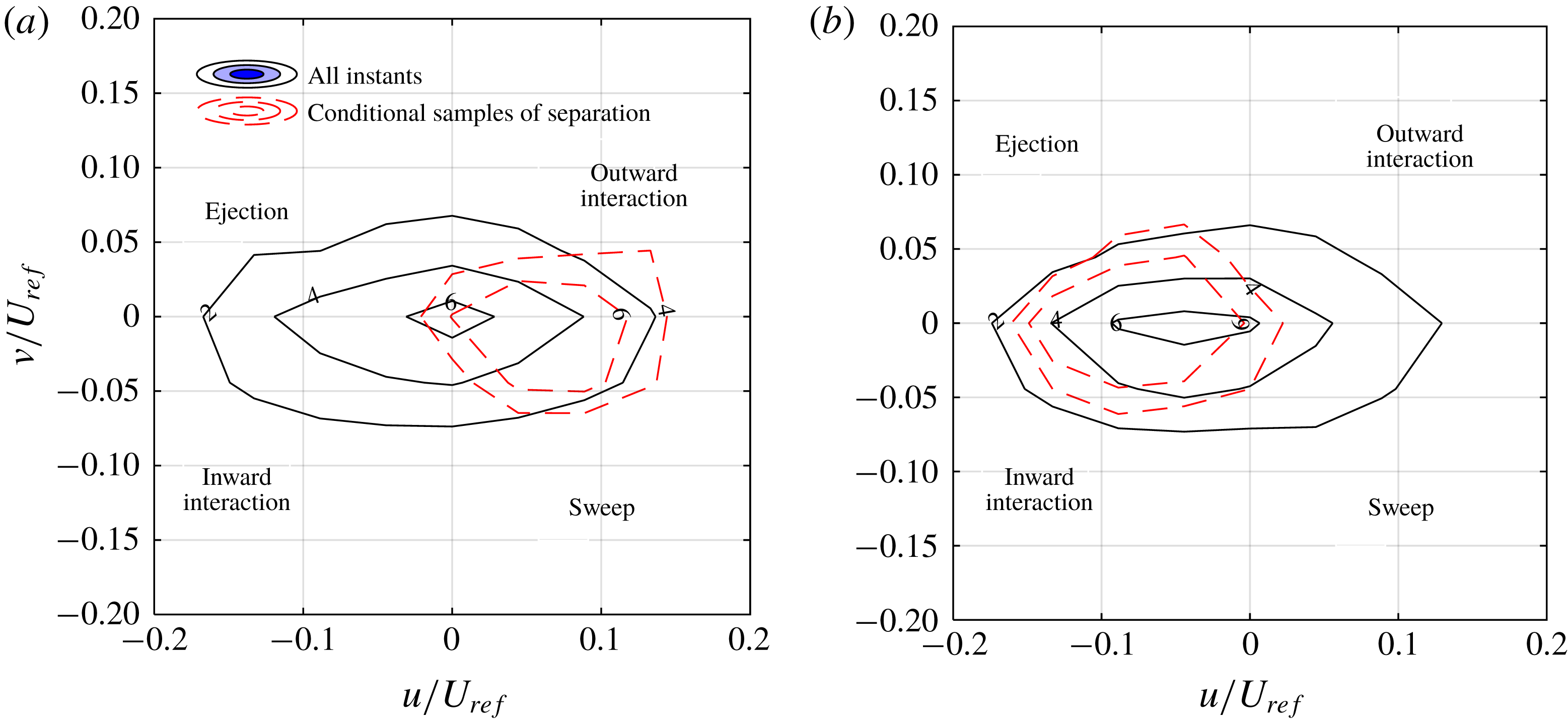
Figure 11. Quadrant distribution of turbulent fluctuations based on all flow instants (solid lines) and the conditional samples of flow with separation (dashed lines) at (a)
 $X=-0.15$
and
$X=-0.15$
and
 $Y=0.03$
, and at (b)
$Y=0.03$
, and at (b)
 $X=0.15$
and
$X=0.15$
and
 $Y=0.03$
. The solid lines represent the regions with probabilities of 2 %, 4 %, and 6 % from the outermost to the innermost contour. The outer and inner dashed lines represent contours with 2 % and 4 % probability, respectively.
$Y=0.03$
. The solid lines represent the regions with probabilities of 2 %, 4 %, and 6 % from the outermost to the innermost contour. The outer and inner dashed lines represent contours with 2 % and 4 % probability, respectively.
The conditional averages demonstrate that flow motions upstream of the separation have a strong positive
 $u$
. Although there are motions with negative or positive
$u$
. Although there are motions with negative or positive
 $v$
, sweep motions with a negative
$v$
, sweep motions with a negative
 $v$
dominate upstream of the separation. The analysis also shows that the motions in the first quadrant, also observed in the past literature, occur as the flow deflects upward to pass over the separation bubble. The separation bubble is dominated by backward flow (
$v$
dominate upstream of the separation. The analysis also shows that the motions in the first quadrant, also observed in the past literature, occur as the flow deflects upward to pass over the separation bubble. The separation bubble is dominated by backward flow (
 $u<0$
), while both ejections and motions of the fourth quadrant are present.
$u<0$
), while both ejections and motions of the fourth quadrant are present.
5 Coherent structures
The energetic structures of the separated flow are identified here using POD of the fluctuating velocity fields (Lumley Reference Lumley, Yaglom and Tatarski1967). The ‘snapshot POD’ method of Sirovich (Reference Sirovich1987) is applied to both the planar and tomo-PIV data to extract the coherent structures with significant contributions to turbulence kinetic energy. The POD of planar PIV is used to analyse a larger FOV and compare the results with other planar analyses in the literature. This is complemented by additional insight into the 3D structures using POD of the tomo-PIV data. The 3D velocity fields are down-sampled by a factor of two to decrease the calculation time and memory requirement for the large set of 1500 volumetric velocity fields. Every instantaneous velocity field is decomposed into a set of orthogonal spatial modes
 $\unicode[STIX]{x1D719}^{i}$
weighted by time-varying amplitudes
$\unicode[STIX]{x1D719}^{i}$
weighted by time-varying amplitudes
 $a_{t}^{i}$
. The mode number is indicated by
$a_{t}^{i}$
. The mode number is indicated by
 $i$
while the amplitudes also depend on time,
$i$
while the amplitudes also depend on time,
 $t$
.
$t$
.
The energy of the first 15 POD modes obtained from planar and tomo-PIV are shown in figure 12. This histogram shows the distribution of energy across the modes, and does not suggest that the 2D and 3D modes are related. The first mode of planar PIV has about 22 % of the total turbulent kinetic energy while the energy of the second mode sharply reduces to 11 %, and to less than 5 % for all other modes. The large energy of the first POD mode relative to the subsequent modes was also observed in APG-induced separation of turbulent wall flow by Mohammed-Taifour & Weiss (Reference Mohammed-Taifour and Weiss2016), in a shock-induced separation by Humble, Scarano & Van Oudheusden (Reference Humble, Scarano and Van Oudheusden2009), and in a geometry-induced separation by Thacker et al. (Reference Thacker, Aubrun, Leroy and Devinant2013). The first POD mode in the investigations of Mohammed-Taifour & Weiss (Reference Mohammed-Taifour and Weiss2016), Humble et al. (Reference Humble, Scarano and Van Oudheusden2009), and Thacker et al. (Reference Thacker, Aubrun, Leroy and Devinant2013) formed 31, 20 and 28 % while the second mode contributes to 9, 5 and 10 % of the total turbulence kinetic energy. However, the first and second 3D modes in figure 12 have closer energies of 24 and 18 %, respectively. The third and the higher order modes of tomo-PIV demonstrate considerably less energy (
 ${<}$
5 %). The shape and the relation of the 2D and 3D modes are investigated in the following.
${<}$
5 %). The shape and the relation of the 2D and 3D modes are investigated in the following.

Figure 12. Energy distribution of POD modes based on planar PIV and tomo-PIV. The energy of each mode is normalized by the total turbulent kinetic energy.
The spatial function of the first two POD modes from planar PIV are shown in figure 13. The vector field of the first mode in figure 13(a) has a uniform direction with the largest vectors located above the separation point. The shape of the mode is similar to the distribution of the Reynolds stresses in figure 6, due to its large contribution to the turbulent kinetic energy. The second POD mode is formed by two diverging regions forming a half-saddle point at
 $X\sim -0.3$
in figure 13(b). This mode has an upstream backward flow and downstream forward flow. High order modes (
$X\sim -0.3$
in figure 13(b). This mode has an upstream backward flow and downstream forward flow. High order modes (
 $i>2$
) with less energy are related to the formation of smaller separation bubbles and smaller structures. These modes are not shown for brevity. Mohammed-Taifour et al. (2016) observed that the low-order velocity field obtained from modes 2 to 50 (excluding the first mode) contain spanwise vortical structures. The phase plot of the amplitude of the first and second modes is shown in figure 13(c) as a scatter plot of
$i>2$
) with less energy are related to the formation of smaller separation bubbles and smaller structures. These modes are not shown for brevity. Mohammed-Taifour et al. (2016) observed that the low-order velocity field obtained from modes 2 to 50 (excluding the first mode) contain spanwise vortical structures. The phase plot of the amplitude of the first and second modes is shown in figure 13(c) as a scatter plot of
 $a^{1}$
versus
$a^{1}$
versus
 $a^{2}$
. The distribution of the amplitudes in this figure shows the lack of any correlation between these two modes. The first mode demonstrates a symmetric distribution of amplitudes while the amplitude distribution of the second mode is skewed toward positive values.
$a^{2}$
. The distribution of the amplitudes in this figure shows the lack of any correlation between these two modes. The first mode demonstrates a symmetric distribution of amplitudes while the amplitude distribution of the second mode is skewed toward positive values.

Figure 13. The spatial organization of the (a) first and (b) second POD modes. The first and second modes represent breathing and shedding motions of the separated flow, respectively. (c) Scatter plot of the distribution of the amplitude of the first and second POD modes for the ensemble of the planar PIV data.
The contribution of the first POD mode from planar PIV to instantaneous flow field is investigated in figure 14 by reconstructing a low-order flow field using the first mode and the mean flow as
 $\langle U\rangle +a_{t}^{1}\unicode[STIX]{x1D719}^{i}$
. The positive and negative amplitudes of
$\langle U\rangle +a_{t}^{1}\unicode[STIX]{x1D719}^{i}$
. The positive and negative amplitudes of
 $a_{t}^{1}=10$
and
$a_{t}^{1}=10$
and
 $-10$
are used in figures 14(a) and 14(b), respectively. The amplitudes are selected based on the distribution observed in figure 13(c). The positive
$-10$
are used in figures 14(a) and 14(b), respectively. The amplitudes are selected based on the distribution observed in figure 13(c). The positive
 $a_{t}^{1}$
extends the backward flow region as seen in figure 14(a). This is observed by comparing the white contour (negative streamwise velocity) with the black line showing the boundaries of the backflow region of the mean flow. The negative
$a_{t}^{1}$
extends the backward flow region as seen in figure 14(a). This is observed by comparing the white contour (negative streamwise velocity) with the black line showing the boundaries of the backflow region of the mean flow. The negative
 $a_{t}^{1}$
in figure 14(b) has reduced the size of the separation bubble and increased the magnitude of the forward flow. Therefore, any variation in the magnitude of
$a_{t}^{1}$
in figure 14(b) has reduced the size of the separation bubble and increased the magnitude of the forward flow. Therefore, any variation in the magnitude of
 $a_{t}^{1}$
changes the size of the backflow region.
$a_{t}^{1}$
changes the size of the backflow region.

Figure 14. A ROM reconstructed using the mean flow and the first POD mode (
 $\langle U\rangle +a_{t}^{1}\unicode[STIX]{x1D719}^{i}$
). Two instants with (a)
$\langle U\rangle +a_{t}^{1}\unicode[STIX]{x1D719}^{i}$
). Two instants with (a)
 $a_{t}^{1}=10$
and (b)
$a_{t}^{1}=10$
and (b)
 $a_{t}^{1}=-10$
are selected. The solid lines show contours of
$a_{t}^{1}=-10$
are selected. The solid lines show contours of
 $\langle U\rangle =0$
from the mean velocity profile of figure 4(a).
$\langle U\rangle =0$
from the mean velocity profile of figure 4(a).
The effect of the second POD mode is investigated in figures 15(a) and 15(b) by reconstructing a low-order model as
 $\langle U\rangle +a_{t}^{2}\unicode[STIX]{x1D719}^{i}$
using
$\langle U\rangle +a_{t}^{2}\unicode[STIX]{x1D719}^{i}$
using
 $a_{t}^{2}=+10$
and
$a_{t}^{2}=+10$
and
 $-10$
, respectively. If the coefficient
$-10$
, respectively. If the coefficient
 $a_{t}^{2}$
is positive, the mode contributes to an upstream backward flow and a downstream forward flow. The superposition of this mode on the mean flow with
$a_{t}^{2}$
is positive, the mode contributes to an upstream backward flow and a downstream forward flow. The superposition of this mode on the mean flow with
 $a_{t}^{2}=+10$
results in an attached flow with a small near-wall velocity across the measurement domain. The boundary layer is thicker at both upstream and downstream locations of
$a_{t}^{2}=+10$
results in an attached flow with a small near-wall velocity across the measurement domain. The boundary layer is thicker at both upstream and downstream locations of
 $X=0$
. If the coefficient
$X=0$
. If the coefficient
 $a_{t}^{2}$
is negative, the second mode contributes to a detachment instant with an upstream forward motion followed by a downstream backward motion as seen in figure 15(b). The second POD mode with
$a_{t}^{2}$
is negative, the second mode contributes to a detachment instant with an upstream forward motion followed by a downstream backward motion as seen in figure 15(b). The second POD mode with
 $a_{t}^{2}=-10$
has resulted in a thicker and larger region of backward flow compared with the mean flow. The angle of the upstream edge of the backward flow region (i.e. shear layer) has also increased due to superposition of the second mode.
$a_{t}^{2}=-10$
has resulted in a thicker and larger region of backward flow compared with the mean flow. The angle of the upstream edge of the backward flow region (i.e. shear layer) has also increased due to superposition of the second mode.

Figure 15. A ROM reconstructed using the mean flow and the second POD mode (
 $\langle U\rangle +a_{t}^{2}\unicode[STIX]{x1D719}^{i}$
). Two instants with (a)
$\langle U\rangle +a_{t}^{2}\unicode[STIX]{x1D719}^{i}$
). Two instants with (a)
 $a_{t}^{2}=10$
and (b)
$a_{t}^{2}=10$
and (b)
 $a_{t}^{2}=-10$
are selected. The solid lines show contours of
$a_{t}^{2}=-10$
are selected. The solid lines show contours of
 $\langle U\rangle =0$
.
$\langle U\rangle =0$
.
The analysis shows that both the first and the second modes of the current planar PIV are associated with breathing motion since they result in expansion/contraction of the backward flow region. The first mode mainly affects the size of the backward flow region in the streamwise direction, while the second mode also affects its wall-normal dimension (thickness). Mohammed-Taifour & Weiss (Reference Mohammed-Taifour and Weiss2016) associated their first POD mode with the expansion and contraction of the separation bubble as it related to the movement of the separation and reattachment points. The mechanism is known as the ‘breathing motion’ and results in low-frequency wall pressure fluctuations (Weiss et al. Reference Weiss, Mohammed-Taifour and Schwaab2015). The difference between the POD modes of the current investigation and Mohammed-Taifour & Weiss (Reference Mohammed-Taifour and Weiss2016) is due to a difference in the size of the FOVs with respect to the separation bubble.
POD of tomo-PIV data demonstrates 3D mechanisms that have been concealed from planar PIV. As was observed in figure 12, the energy of the first POD modes of tomo-PIV is only about 30 % larger than that of the second mode, while the energy of the first POD mode of planar PIV is at least twice as large as that of the second mode. Inspection of the first and second POD modes from tomo-PIV from figure 16(a,b) shows that the spatial function of the first and the second POD modes are similar. These two modes have a high-velocity core while the 3D streamlines show a strong spanwise component. The first mode shows a forward flow and the second mode shows a backward flow, although their direction in reconstruction of an instantaneous flow field depends on the sign of
 $a_{t}^{1}$
or
$a_{t}^{1}$
or
 $a_{t}^{2}$
. By varying the amplitude of the coefficients, the modes can also contribute to expansion and contraction of the backward flow region. The strong spanwise component was not detectable in the breathing motion described by planar PIV of the current investigation and POD analysis of Mohammed-Taifour & Weiss (Reference Mohammed-Taifour and Weiss2016). Spanwise motion is an inherent characteristic of any separated flow in a 3D domain. Flow tends to escape in the spanwise direction to reduce the streamwise deceleration when it encounters APG (Délery Reference Délery2013). These two POD modes from tomo-PIV indicate that large-scale streamwise and spanwise motions simultaneously occur and form most of the turbulent kinetic energy of the flow. The evolution of the amplitude of the first and the second POD modes from tomo-PIV (
$a_{t}^{2}$
. By varying the amplitude of the coefficients, the modes can also contribute to expansion and contraction of the backward flow region. The strong spanwise component was not detectable in the breathing motion described by planar PIV of the current investigation and POD analysis of Mohammed-Taifour & Weiss (Reference Mohammed-Taifour and Weiss2016). Spanwise motion is an inherent characteristic of any separated flow in a 3D domain. Flow tends to escape in the spanwise direction to reduce the streamwise deceleration when it encounters APG (Délery Reference Délery2013). These two POD modes from tomo-PIV indicate that large-scale streamwise and spanwise motions simultaneously occur and form most of the turbulent kinetic energy of the flow. The evolution of the amplitude of the first and the second POD modes from tomo-PIV (
 $a_{t}^{1}$
or
$a_{t}^{1}$
or
 $a_{t}^{2}$
) are shown in figure 17. Although both of these modes represent spanwise motion, they appear to be independent and uncorrelated.
$a_{t}^{2}$
) are shown in figure 17. Although both of these modes represent spanwise motion, they appear to be independent and uncorrelated.

Figure 16. 3D spatial organization of POD modes obtained from tomo-PIV showing the (a) first, (b) second, (c) third, (d) fourth, (e) fifth and (f) sixth most energetic modes. The dark grey (blue online), bright grey (yellow online) and medium grey (green online) contours represent isosurfaces of normalized magnitude of the mode magnitude at
 $|\unicode[STIX]{x1D719}^{i}|=0.0033$
, 0.0025 and 0.0012, respectively. The streamlines visualize the 3D spatial pattern of the modes.
$|\unicode[STIX]{x1D719}^{i}|=0.0033$
, 0.0025 and 0.0012, respectively. The streamlines visualize the 3D spatial pattern of the modes.

Figure 17. Phase diagram of the amplitude of the first and the second POD modes from tomo-PIV. Both modes have a strong spanwise motion.
The third POD mode in figure 16(c) represents a focus-type structure with a low velocity core centred at
 $Z=0$
and
$Z=0$
and
 $X=-0.1$
. There is a critical point at the centre of the focus with zero wall shear stress (i.e.
$X=-0.1$
. There is a critical point at the centre of the focus with zero wall shear stress (i.e.
 $\unicode[STIX]{x1D70F}_{w,x}=\unicode[STIX]{x1D70F}_{w,z}=0$
). The focus structure in figure 16(c) is stretched in the streamwise direction while its axis is slightly inclined in the positive
$\unicode[STIX]{x1D70F}_{w,x}=\unicode[STIX]{x1D70F}_{w,z}=0$
). The focus structure in figure 16(c) is stretched in the streamwise direction while its axis is slightly inclined in the positive
 $X$
direction. The fourth POD mode in figure 16(d) shows a saddle structure with streamlines diverging from the separation line. The separation line is indicated with a dashed line and is of the attachment type. This line passes through a saddle point that is not visible within the FOV. The fifth POD mode in figure 16(e) is also a saddle structure. The attachment-type separation line of this saddle point with diverging streamlines and the detachment-type separation line with converging streamlines are indicated in this figure. In an
$X$
direction. The fourth POD mode in figure 16(d) shows a saddle structure with streamlines diverging from the separation line. The separation line is indicated with a dashed line and is of the attachment type. This line passes through a saddle point that is not visible within the FOV. The fifth POD mode in figure 16(e) is also a saddle structure. The attachment-type separation line of this saddle point with diverging streamlines and the detachment-type separation line with converging streamlines are indicated in this figure. In an
 $XY$
plane perpendicular to the attachment line, these modes form a half-saddle structure with diverging streamlines. The sixth POD mode in figure 16(f) consists of a saddle point with two distinguished separation lines crossing
$XY$
plane perpendicular to the attachment line, these modes form a half-saddle structure with diverging streamlines. The sixth POD mode in figure 16(f) consists of a saddle point with two distinguished separation lines crossing
 $(X,Z)=(0,0)$
. The streamlines split around the
$(X,Z)=(0,0)$
. The streamlines split around the
 $X=0$
line and converge about the attachment line on the two sides of
$X=0$
line and converge about the attachment line on the two sides of
 $Z=0$
. The higher-order modes with smaller energy contain more complex and asymmetric structures, which are not shown for brevity.
$Z=0$
. The higher-order modes with smaller energy contain more complex and asymmetric structures, which are not shown for brevity.
The first and second POD modes from tomo-PIV do not contain a critical point while they can form a separation bubble or generate a significant spanwise motion. The third mode forms a focus structure similar to the mean flow pattern. The fourth, fifth and six POD modes show saddle structures, which are associated with flow separation. The role and the interaction of these modes in the mechanism of the separation are investigated using a ROM in the next section.
6 The separation mechanism
A ROM is developed based on POD modes of tomo-PIV data and conditionally averaged amplitude (
 $\langle a_{t}^{i}\rangle _{c}$
) of the POD modes. The modeling takes advantage of the relatively time-resolved acquisition frequency of the tomo-PIV with
$\langle a_{t}^{i}\rangle _{c}$
) of the POD modes. The modeling takes advantage of the relatively time-resolved acquisition frequency of the tomo-PIV with
 $\unicode[STIX]{x0394}t=400$
ms between tomo-PIV vector fields. Assuming an average advection velocity of
$\unicode[STIX]{x0394}t=400$
ms between tomo-PIV vector fields. Assuming an average advection velocity of
 $0.04U_{\infty }$
(
$0.04U_{\infty }$
(
 $0.02~\text{m}~\text{s}^{-1}$
) in the FOV of tomo-PIV, the turbulence structures are expected to travel about
$0.02~\text{m}~\text{s}^{-1}$
) in the FOV of tomo-PIV, the turbulence structures are expected to travel about
 $0.05H$
(8 mm) equivalent to
$0.05H$
(8 mm) equivalent to
 ${\sim}$
9 % of the tomo-PIV domain between two consecutive acquisitions in the
${\sim}$
9 % of the tomo-PIV domain between two consecutive acquisitions in the
 $X$
direction. Therefore, conditional averages of the amplitudes of the first six POD modes (
$X$
direction. Therefore, conditional averages of the amplitudes of the first six POD modes (
 $a_{t}^{i}$
,
$a_{t}^{i}$
,
 $i=1$
–6) are obtained within a time interval of
$i=1$
–6) are obtained within a time interval of
 $-6\unicode[STIX]{x0394}t$
to
$-6\unicode[STIX]{x0394}t$
to
 $+6\unicode[STIX]{x0394}t$
of the separation instant (
$+6\unicode[STIX]{x0394}t$
of the separation instant (
 $t_{0}$
) to characterize the temporal behaviour. The conditionally averaged amplitudes are indicated as
$t_{0}$
) to characterize the temporal behaviour. The conditionally averaged amplitudes are indicated as
 $\langle a_{t0+n\unicode[STIX]{x0394}t}^{i}\rangle _{c}$
, where
$\langle a_{t0+n\unicode[STIX]{x0394}t}^{i}\rangle _{c}$
, where
 $n$
is an integer ranging from
$n$
is an integer ranging from
 $-6$
to
$-6$
to
 $+6$
. The result is shown in figure 18 as a function of normalized time
$+6$
. The result is shown in figure 18 as a function of normalized time
 $T=(t-t_{0})/\unicode[STIX]{x0394}t$
. The coefficients of the first and the second modes (i.e.
$T=(t-t_{0})/\unicode[STIX]{x0394}t$
. The coefficients of the first and the second modes (i.e.
 $\langle a^{1}\rangle _{c}$
and
$\langle a^{1}\rangle _{c}$
and
 $\langle a^{2}\rangle _{c}$
) undergo a rapid increase and reach a maximum value at
$\langle a^{2}\rangle _{c}$
) undergo a rapid increase and reach a maximum value at
 $T=1$
and
$T=1$
and
 $T=0$
(separation instant), respectively. The coefficients of the fourth and the sixth modes also show a local minimum at
$T=0$
(separation instant), respectively. The coefficients of the fourth and the sixth modes also show a local minimum at
 $T=0$
. In order to visualize the combined effect of the modes, the conditionally averaged coefficients from figure 18 are applied to reconstruct a low-order 3D model as
$T=0$
. In order to visualize the combined effect of the modes, the conditionally averaged coefficients from figure 18 are applied to reconstruct a low-order 3D model as
 $$\begin{eqnarray}\displaystyle \tilde{U} _{t_{0}+n\unicode[STIX]{x0394}t}=\langle \boldsymbol{U}\rangle +\mathop{\sum }_{i=1}^{6}\langle a_{t_{0}+n\unicode[STIX]{x0394}t}^{i}\rangle _{c}\unicode[STIX]{x1D753}^{i}. & & \displaystyle\end{eqnarray}$$

Figure 18. Conditional average of POD coefficients (
 $\langle a_{T}^{i}\rangle _{c}$
) before and after the flow separation instant.
$\langle a_{T}^{i}\rangle _{c}$
) before and after the flow separation instant.
The reconstructed low-order model of the separation mechanism from
 $T=-3$
to
$T=-3$
to
 $+2$
are shown in figures 19(a) to 19(f), respectively. A large focus structure, centred at the corner of the FOV at about
$+2$
are shown in figures 19(a) to 19(f), respectively. A large focus structure, centred at the corner of the FOV at about
 $X=0.2$
and
$X=0.2$
and
 $Z=-0.2$
, is observed at the
$Z=-0.2$
, is observed at the
 $T=-3$
instant of figure 19(a). The focus pattern induces a backward streamwise motion in most of the FOV. The relatively large negative value of
$T=-3$
instant of figure 19(a). The focus pattern induces a backward streamwise motion in most of the FOV. The relatively large negative value of
 $\langle a^{1}\rangle _{c}$
at
$\langle a^{1}\rangle _{c}$
at
 $T=-3$
in figure 18 shows that the first mode is the main contributor to the backward flow. A similar flow pattern is observed at
$T=-3$
in figure 18 shows that the first mode is the main contributor to the backward flow. A similar flow pattern is observed at
 $T=-2$
of figure 19(b) although the coefficient of the second mode,
$T=-2$
of figure 19(b) although the coefficient of the second mode,
 $\langle a^{2}\rangle _{c}$
, has rapidly increased. With a further increase of
$\langle a^{2}\rangle _{c}$
, has rapidly increased. With a further increase of
 $\langle a^{2}\rangle _{c}$
and a reduction of
$\langle a^{2}\rangle _{c}$
and a reduction of
 $\langle a^{1}\rangle _{c}$
at
$\langle a^{1}\rangle _{c}$
at
 $T=-1$
, a saddle-point structure forms in figure 19(c). The saddle-point structure is further established at the separation instant (
$T=-1$
, a saddle-point structure forms in figure 19(c). The saddle-point structure is further established at the separation instant (
 $T=0$
), while the coefficients of modes four, five and six reach a local extrema. The saddle-point structure confirms the presence of a 3D separated flow at this instant, which is in agreement with the conditional sampling. The flow pattern in figure 19(d) demonstrates a forward flow at
$T=0$
), while the coefficients of modes four, five and six reach a local extrema. The saddle-point structure confirms the presence of a 3D separated flow at this instant, which is in agreement with the conditional sampling. The flow pattern in figure 19(d) demonstrates a forward flow at
 $X<0$
and a backward flow at
$X<0$
and a backward flow at
 $X>0$
along the
$X>0$
along the
 $Z=0$
as enforced by the conditional sampling. The streamlines converge along the separation line which is inclined with respect to the spanwise direction. Immediately after the separation instant, a focus-type structure appears in figure 19(e) and further moves into the FOV at
$Z=0$
as enforced by the conditional sampling. The streamlines converge along the separation line which is inclined with respect to the spanwise direction. Immediately after the separation instant, a focus-type structure appears in figure 19(e) and further moves into the FOV at
 $T=2$
of figure 19(f). The centre of the vortical structure is at about
$T=2$
of figure 19(f). The centre of the vortical structure is at about
 $(X,Z)=(-0.2,0.1)$
, which is the opposite corner of the FOV relative to the focus centre before separation in figure 19(a). The ROM shows that the separated flow is formed by a saddle-point structure, which interacts with foci structures.
$(X,Z)=(-0.2,0.1)$
, which is the opposite corner of the FOV relative to the focus centre before separation in figure 19(a). The ROM shows that the separated flow is formed by a saddle-point structure, which interacts with foci structures.

Figure 19. A low-order model of the flow motions before and after the separation instant (
 $T=0$
) using the first six POD modes of tomo-PIV and conditionally averaged coefficients. The flow is shown at (a)
$T=0$
) using the first six POD modes of tomo-PIV and conditionally averaged coefficients. The flow is shown at (a)
 $T=-3$
with contours of
$T=-3$
with contours of
 $|U|=0.067U_{ref}$
(blue online/dark grey) and
$|U|=0.067U_{ref}$
(blue online/dark grey) and
 $0.044U_{ref}$
(yellow online/light grey), (b) at
$0.044U_{ref}$
(yellow online/light grey), (b) at
 $T=-2$
with contours of
$T=-2$
with contours of
 $|U|=0.044U_{ref}$
(blue online/dark grey) and
$|U|=0.044U_{ref}$
(blue online/dark grey) and
 $0.0156U_{ref}$
(yellow online/light grey), (c) at
$0.0156U_{ref}$
(yellow online/light grey), (c) at
 $T=-1$
with contours of
$T=-1$
with contours of
 $|U|=0.067U_{ref}$
(blue online/dark grey) and
$|U|=0.067U_{ref}$
(blue online/dark grey) and
 $0.044U_{ref}$
(yellow online/light grey), (d) at
$0.044U_{ref}$
(yellow online/light grey), (d) at
 $T=0$
with contours of
$T=0$
with contours of
 $|U|=0.067U_{ref}$
(blue online/dark grey) and
$|U|=0.067U_{ref}$
(blue online/dark grey) and
 $0.044U_{c}$
(yellow online/light grey), at (e)
$0.044U_{c}$
(yellow online/light grey), at (e)
 $T=1$
with contours of
$T=1$
with contours of
 $|U|=0.044U_{ref}$
(blue online/dark grey) and
$|U|=0.044U_{ref}$
(blue online/dark grey) and
 $0.011U_{ref}$
(yellow online/light grey), and at (f)
$0.011U_{ref}$
(yellow online/light grey), and at (f)
 $T=2$
with contours of
$T=2$
with contours of
 $|U|=0.044U_{ref}$
(blue online/dark grey) and
$|U|=0.044U_{ref}$
(blue online/dark grey) and
 $0.016U_{ref}$
(yellow online/light grey).
$0.016U_{ref}$
(yellow online/light grey).
7 Discussion and conclusions
The 3D separation of a TBL induced by an APG over an asymmetric flat diffuser is investigated to identify the turbulent structures and the mechanism of flow separation. A planar PIV with a high spatial dynamic range is applied to cover a large domain in a streamwise wall-normal plane and provides a base for comparison with previous literature on the turbulence statistics of APG-induced separation. Volumetric measurement using tomo-PIV was also carried out to capture the 3D turbulent structures.
The average flow field at the mid-span of the diffuser consisted of a spiral motion with a wall-normal axis of rotation and an elliptical cross-section. The major axis of the elliptical vortex was tilted with respect to the streamwise direction. This resulted in a strong forward flow upstream of the focus point and a weaker backward flow downstream of the focus point, as also observed in the streamwise wall-normal measurement plane of planar PIV. The flow upstream of the focus point maintains its forward direction most of the time while the flow downstream of the separation point has a small intermittency factor (
 $\unicode[STIX]{x1D6FE}$
) with a larger probability of backward flow. The conditional averaging of the separation instants from planar and tomo-PIV shows that the strengths of the forward and backflow flow on the two sides of an instantaneous separation are equivalent. The separation front in the conditional average of tomo-PIV data is extended in the spanwise direction across the measurement domain. The 3D streamlines of the conditional average form a saddle-point structure in the streamwise–spanwise plane with converging streamlines. The spanwise convergence of the streamlines of this structure indicates lift-up and separation of the flow from the surface.
$\unicode[STIX]{x1D6FE}$
) with a larger probability of backward flow. The conditional averaging of the separation instants from planar and tomo-PIV shows that the strengths of the forward and backflow flow on the two sides of an instantaneous separation are equivalent. The separation front in the conditional average of tomo-PIV data is extended in the spanwise direction across the measurement domain. The 3D streamlines of the conditional average form a saddle-point structure in the streamwise–spanwise plane with converging streamlines. The spanwise convergence of the streamlines of this structure indicates lift-up and separation of the flow from the surface.
The movement of the separation point does allow formation of a separation bubble with small turbulence intensity in the planar distributions of normal and shear Reynolds stresses. In general, high Reynolds stresses are observed away from the wall, while the peak intensity linearly moves away from the wall with an increase of the streamwise distance. The large Reynolds shear stresses are associated with correlated
 $u$
and
$u$
and
 $v$
fluctuations due to the roll-up of the shear layer into vortical structures. The triple products of turbulent fluctuations also show that the high turbulence kinetic energy of the separated shear layer is transported toward the wall by sweep and away from the wall by ejection motions.
$v$
fluctuations due to the roll-up of the shear layer into vortical structures. The triple products of turbulent fluctuations also show that the high turbulence kinetic energy of the separated shear layer is transported toward the wall by sweep and away from the wall by ejection motions.
The conditional averages of separation instants show a separation bubble with small streamwise Reynolds stress,
 $\langle u^{2}\rangle$
. A region of positive Reynolds shear stress is observed upstream of the separation point, which results in negative turbulence production. The analysis shows that the positive Reynolds shear stress is due to the upward deflection of the upstream streamlines to pass over the separation bubble. These motions are characterized with
$\langle u^{2}\rangle$
. A region of positive Reynolds shear stress is observed upstream of the separation point, which results in negative turbulence production. The analysis shows that the positive Reynolds shear stress is due to the upward deflection of the upstream streamlines to pass over the separation bubble. These motions are characterized with
 $u>0$
and
$u>0$
and
 $v>0$
of the first
$v>0$
of the first
 $u$
–
$u$
–
 $v$
quadrant, and continue above the separation bubble. The transport of turbulent kinetic energy upstream of the separation point is mainly carried out by the sweep motions, while ejections and motions of the third
$v$
quadrant, and continue above the separation bubble. The transport of turbulent kinetic energy upstream of the separation point is mainly carried out by the sweep motions, while ejections and motions of the third
 $u$
–
$u$
–
 $v$
quadrant (
$v$
quadrant (
 $u<0$
and
$u<0$
and
 $v<0$
) dominate downstream of the separation point.
$v<0$
) dominate downstream of the separation point.
The POD of the volumetric realizations from tomo-PIV show that about 42 % of the turbulence kinetic energy is due to large-scale streamwise fluctuations with a strong spanwise component. These motions are captured by the first two POD modes, which have a similar energy level. The other high-order POD modes include focus and saddle-point structures. A ROM is developed using the sixth dominant 3D modes of POD and their averaged amplitudes obtained from conditional sampling of the separation instants. The ROM shows that the separation instant has a saddle-point structure with converging streamlines along its separation line.


