3.1 The approximate solution to the Laplace equation

Agnon et al. (Reference Agnon, Madsen and Schäffer1999) truncated (2.7)–(2.9) at fifth order, by which the velocity field and the associated velocity potential simplified to

(3.1)$$\begin{eqnarray}\displaystyle & \displaystyle u[x,z,t]=\left(1-\frac{z^{2}}{2}\unicode[STIX]{x1D6FB}^{2}+\frac{z^{4}}{24}\unicode[STIX]{x1D6FB}^{4}\right)u_{0}+\left(z\unicode[STIX]{x1D735}-\frac{z^{3}}{6}\unicode[STIX]{x1D6FB}^{3}+\frac{z^{5}}{120}\unicode[STIX]{x1D6FB}^{5}\right)w_{0}, & \displaystyle\end{eqnarray}$$

(3.2)$$\begin{eqnarray}\displaystyle & \displaystyle w[x,z,t]=\left(1-\frac{z^{2}}{2}\unicode[STIX]{x1D6FB}^{2}+\frac{z^{4}}{24}\unicode[STIX]{x1D6FB}^{4}\right)w_{0}-\left(z\unicode[STIX]{x1D735}-\frac{z^{3}}{6}\unicode[STIX]{x1D6FB}^{3}+\frac{z^{5}}{120}\unicode[STIX]{x1D6FB}^{5}\right)u_{0}, & \displaystyle\end{eqnarray}$$

(3.3)$$\begin{eqnarray}\displaystyle & \displaystyle \unicode[STIX]{x1D6F7}[x,z,t]=\left(1-\frac{z^{2}}{2}\unicode[STIX]{x1D6FB}^{2}+\frac{z^{4}}{24}\unicode[STIX]{x1D6FB}^{4}\right)\unicode[STIX]{x1D6F7}_{0}+\left(z-\frac{z^{3}}{6}\unicode[STIX]{x1D6FB}^{2}+\frac{z^{5}}{120}\unicode[STIX]{x1D6FB}^{4}\right)w_{0}. & \displaystyle\end{eqnarray}$$

In order to satisfy the kinematic bottom condition (2.10), they utilized (3.2) with $z=-h$, but Padé enhanced the resulting equation to obtain

(3.4)$$\begin{eqnarray}\left(1-{\textstyle \frac{4}{9}}h^{2}\unicode[STIX]{x1D6FB}^{2}+{\textstyle \frac{1}{63}}h^{4}\unicode[STIX]{x1D6FB}^{4}\right)w_{0}+\left(h\unicode[STIX]{x1D6FB}-{\textstyle \frac{1}{9}}h^{3}\unicode[STIX]{x1D6FB}^{3}+{\textstyle \frac{1}{945}}h^{5}\unicode[STIX]{x1D6FB}^{5}\right)u_{0}=0.\end{eqnarray}$$

Finally, the connection to the surface variables was established by using (3.1)–(3.3) with $z=\unicode[STIX]{x1D702}$, leading to

(3.5)$$\begin{eqnarray}\displaystyle & \displaystyle u_{s}=\left(1-{\textstyle \frac{1}{2}}\unicode[STIX]{x1D702}^{2}\unicode[STIX]{x1D6FB}^{2}+{\textstyle \frac{1}{24}}\unicode[STIX]{x1D702}^{4}\unicode[STIX]{x1D6FB}^{4}\right)u_{0}+\left(\unicode[STIX]{x1D702}\unicode[STIX]{x1D735}-{\textstyle \frac{1}{6}}\unicode[STIX]{x1D702}^{3}\unicode[STIX]{x1D6FB}^{3}+{\textstyle \frac{1}{120}}\unicode[STIX]{x1D702}^{5}\unicode[STIX]{x1D6FB}^{5}\right)w_{0}, & \displaystyle\end{eqnarray}$$

(3.6)$$\begin{eqnarray}\displaystyle & \displaystyle w_{s}=\left(1-{\textstyle \frac{1}{2}}\unicode[STIX]{x1D702}^{2}\unicode[STIX]{x1D6FB}^{2}+{\textstyle \frac{1}{24}}\unicode[STIX]{x1D702}^{4}\unicode[STIX]{x1D6FB}^{4}\right)w_{0}-\left(\unicode[STIX]{x1D702}\unicode[STIX]{x1D735}-{\textstyle \frac{1}{6}}\unicode[STIX]{x1D702}^{3}\unicode[STIX]{x1D6FB}^{3}+{\textstyle \frac{1}{120}}\unicode[STIX]{x1D702}^{5}\unicode[STIX]{x1D6FB}^{5}\right)u_{0}, & \displaystyle\end{eqnarray}$$

(3.7)$$\begin{eqnarray}\displaystyle & \displaystyle \unicode[STIX]{x1D6F7}_{s}=\left(1-{\textstyle \frac{1}{2}}\unicode[STIX]{x1D702}^{2}\unicode[STIX]{x1D6FB}^{2}+{\textstyle \frac{1}{24}}\unicode[STIX]{x1D702}^{4}\unicode[STIX]{x1D6FB}^{4}\right)\unicode[STIX]{x1D6F7}_{0}+\left(\unicode[STIX]{x1D702}-{\textstyle \frac{1}{6}}\unicode[STIX]{x1D702}^{3}\unicode[STIX]{x1D6FB}^{2}+{\textstyle \frac{1}{120}}\unicode[STIX]{x1D702}^{5}\unicode[STIX]{x1D6FB}^{4}\right)w_{0}. & \displaystyle\end{eqnarray}$$

It should be noted that Agnon et al. (Reference Agnon, Madsen and Schäffer1999) actually only considered a fourth-order connection in (3.5)–(3.7), i.e. they did not include the terms proportional to $\unicode[STIX]{x1D6FB}^{5}$. In the following, however, we shall analyse both the fifth-order and the fourth-order formulations.

3.2 Analysis of the embedded linear dispersion relation

The linear dispersion relation embedded in the formulation by Agnon et al. (Reference Agnon, Madsen and Schäffer1999) is analysed by looking for harmonic solutions of the form

(3.8a-c)$$\begin{eqnarray}\unicode[STIX]{x1D702}=\unicode[STIX]{x1D700}A_{0}\cos [kx-\unicode[STIX]{x1D714}t],\quad u_{0}=\unicode[STIX]{x1D700}B_{0}\cos [kx-\unicode[STIX]{x1D714}t],\quad w_{0}=\unicode[STIX]{x1D700}C_{0}\sin [kx-\unicode[STIX]{x1D714}t],\end{eqnarray}$$

where $\unicode[STIX]{x1D700}\ll 1$. First of all, equation (3.4) directly leads to the connection

(3.9)$$\begin{eqnarray}C_{0}=B_{0}F_{0}[\unicode[STIX]{x1D705}],\end{eqnarray}$$

with

(3.10a,b)$$\begin{eqnarray}F_{0}[\unicode[STIX]{x1D705}]\equiv \unicode[STIX]{x1D705}\left(\frac{1+\frac{1}{9}\unicode[STIX]{x1D705}^{2}+\frac{1}{945}\unicode[STIX]{x1D705}^{4}}{1+\frac{4}{9}\unicode[STIX]{x1D705}^{2}+\frac{1}{63}\unicode[STIX]{x1D705}^{4}}\right)\quad \text{and}\quad \unicode[STIX]{x1D705}\equiv kh.\end{eqnarray}$$

Second, by inserting (3.8) into (3.5)–(3.6) and collecting terms of order $O(\unicode[STIX]{x1D700})$, we obtain the leading-order approximations $u_{s}\simeq u_{0}$, $w_{s}\simeq w_{0}$, while (2.6) leads to $V_{s}\simeq u_{0}$. Consequently (2.3) and (2.5) lead to the homogeneous problem

(3.11)$$\begin{eqnarray}\left(\begin{array}{@{}cc@{}}\unicode[STIX]{x1D714}m_{11} & m_{12}\\ m_{21} & \unicode[STIX]{x1D714}m_{22}\end{array}\right)\left(\begin{array}{@{}c@{}}A_{0}\\ B_{0}\end{array}\right)=\left(\begin{array}{@{}c@{}}0\\ 0\end{array}\right),\end{eqnarray}$$

with

(3.12a-d)$$\begin{eqnarray}m_{11}=1,\quad m_{12}=-F_{0}[\unicode[STIX]{x1D705}],\quad m_{21}=-gk,\quad m_{22}=1.\end{eqnarray}$$

The homogeneous problem requires the determinant of the matrix in (3.11) to be zero, and this leads to the dispersion relation

(3.13)$$\begin{eqnarray}\frac{c^{2}}{gh}\equiv \frac{\unicode[STIX]{x1D714}^{2}}{k^{2}gh}=\frac{F_{0}[\unicode[STIX]{x1D705}]}{\unicode[STIX]{x1D705}}.\end{eqnarray}$$

Using a threshold of 2 % error compared to the fully dispersive target, equation (3.13) turns out to be applicable up to $kh=6.2$.

3.3 Numerical implementation on a constant depth

From our experience with modelling nonlinear regular and irregular waves, it appears that ‘mysterious’ numerical blowups can originate in relatively deep troughs of the overall surface elevation whenever the Nyquist wave number is high. In order to demonstrate this problem, we first implement a spectral model solving the equations by Agnon et al. (Reference Agnon, Madsen and Schäffer1999) on a constant depth. The time stepping of (2.3)–(2.4) is based on a fourth-order Runge–Kutta method, and all spatial derivatives are handled by spectral representations involving a toggling from physical space to Fourier space and back into physical space by using fast Fourier transforms. We represent the solution in $k$-space by considering $N$ discrete wavenumbers ($k_{j}=j\unicode[STIX]{x0394}k$, with $j=1,2,\ldots ,N$) and $N_{x}=2N$ grid points ($x_{i}=i\unicode[STIX]{x0394}x$, with $i=1,2,\ldots ,N_{x}$). The Nyquist wavenumber is determined by $k_{N}=\unicode[STIX]{x03C0}/\unicode[STIX]{x0394}x$.

Within each of the four sub-time steps in the Runge–Kutta procedure, we need to determine $w_{s}$ on the basis of ($\unicode[STIX]{x1D702}$, $\unicode[STIX]{x1D6F7}_{s}$) known at all grid points. First, $(\unicode[STIX]{x1D6F7}_{0},u_{0},w_{0})$ are described by

(3.14)$$\begin{eqnarray}\displaystyle & \displaystyle \unicode[STIX]{x1D6F7}_{0}[x]=a_{0}+\mathop{\sum }_{j=1}^{N}\left(a_{j}\sin [k_{j}x]-b_{j}\cos [k_{j}x]\right), & \displaystyle\end{eqnarray}$$

(3.15)$$\begin{eqnarray}\displaystyle & \displaystyle u_{0}[x]=\mathop{\sum }_{j=1}^{N}k_{j}\left(a_{j}\cos [k_{j}x]+b_{j}\sin [k_{j}x]\right), & \displaystyle\end{eqnarray}$$

(3.16)$$\begin{eqnarray}\displaystyle & \displaystyle w_{0}[x]=\mathop{\sum }_{j=1}^{N}k_{j}F_{0}[k_{j}h]\left(a_{j}\sin [k_{j}x]-b_{j}\cos [k_{j}x]\right), & \displaystyle\end{eqnarray}$$

with $a_{N}\equiv 0$. Second, equation (3.7) is satisfied in each grid point, which leads to $2N$ linear equations with the unknowns $a_{j}$ and $b_{j}$ for $j=1,2,\ldots ,N$. This problem is solved in Mathematica by invoking the linear matrix solver LinearSolve. Finally, $w_{s}$ is determined using (3.6).

With the numerical model at hand, we first make a simulation of a standing wave problem defined by the initial conditions

(3.17a,b)$$\begin{eqnarray}\unicode[STIX]{x1D702}/h=\unicode[STIX]{x1D707}\cos [k_{1}x]\quad \text{and}\quad \unicode[STIX]{x1D6F7}_{s}=0,\end{eqnarray}$$

with amplitude $\unicode[STIX]{x1D707}=0.05$, water depth $h=1$ m and domain size $L=2\unicode[STIX]{x03C0}$. The spectral and numerical resolution for this simulation is chosen as

(3.18a-e)$$\begin{eqnarray}N=10,\quad k_{1}h=1.0,\quad k_{N}h=10,\quad N_{x}=20,\quad \unicode[STIX]{x0394}x=\unicode[STIX]{x03C0}/10\text{ m,}\end{eqnarray}$$

with the time step $\unicode[STIX]{x0394}t\,=\,0.04$ s corresponding to a Courant number $C_{r}\,\equiv \,\unicode[STIX]{x0394}t\,\sqrt{gh}/\unicode[STIX]{x0394}x\,=0.4$. This simulation runs for $500$ time steps (approximately ten wave periods) without showing any signs of instability.

Then, to illustrate the problem of trough instabilities, we maintain the same initial conditions as above, but change the spectral and numerical resolution to

(3.19a-e)$$\begin{eqnarray}N=40,\quad k_{1}h=1.0,\quad k_{N}h=40,\quad N_{x}=80,\quad \unicode[STIX]{x0394}x=\unicode[STIX]{x03C0}/40\text{ m,}\end{eqnarray}$$

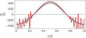
with the time step of $\unicode[STIX]{x0394}t=0.01$ s leading again to $C_{r}=0.4$. This time the simulation starts to go unstable after approximately $89$ time steps (shown as the black curve in figure 1). It is obvious that the instability evolves from the trough of the wave. After $95$ time steps (shown as the red curve in figure 1), the instability has expanded to the complete profile and soon after the simulation blows up. It appears that the value of $k_{N}h$ is important for the instability just observed.

Figure 1. Numerical solution to the formulation by Agnon et al. (Reference Agnon, Madsen and Schäffer1999) with fourth-order operators. Input given by (3.17) and (3.19). Black line: surface elevation after 89 time steps. Red line: surface elevation after 95 time steps.

Figure 2. Numerical solution to the formulation by Agnon et al. (Reference Agnon, Madsen and Schäffer1999) with fourth-order operators. Input given by (3.20) and (3.19). Black line: surface elevation after 60 time steps.

In order to study the trough instability in more detail, we modify the initial conditions to

(3.20a,b)$$\begin{eqnarray}\unicode[STIX]{x1D702}/h=\unicode[STIX]{x1D6FF}+\unicode[STIX]{x1D707}\cos [k_{1}x]\quad \text{and}\quad \unicode[STIX]{x1D6F7}_{s}=0,\end{eqnarray}$$

where $\unicode[STIX]{x1D6FF}=-0.05$, $\unicode[STIX]{x1D707}=0.005$ and $h=1~\text{m}$. This represents a perturbation, having amplitude ten times smaller than the previous wave and which runs with a negative offset $\unicode[STIX]{x1D6FF}$ equal to the trough of the previous wave. Again the numerical set-up is given by (3.19). As shown in figure 2, this simulation starts to go unstable after approximately $60$ time steps. It is, however, possible to spot the growing instability at a much earlier stage by monitoring the complex $k$-spectrum of the surface elevation (shown in figure 3 after $40$ time steps). The horizontal axis is $k_{j}h$ with $j=1,2,\ldots ,N$. The spectrum shows very clearly that an instability is evolving at $k_{j}h=18$. With this procedure, we are now able to detect the critical wavenumbers for any value of $\unicode[STIX]{x1D6FF}$. This will be utilized in the following sections.

Figure 3. Absolute values of the complex $k$-spectrum for the surface elevation after 40 time steps. Input given by (3.20) and (3.19).

3.4 Analysis of trough instabilities

A simple analysis of the trough instability illustrated in figures 1–3 can be conducted by modifying (3.8) to

(3.21a-c)$$\begin{eqnarray}\unicode[STIX]{x1D702}=\unicode[STIX]{x1D6FF}h+\unicode[STIX]{x1D700}A_{0}\cos [kx-\unicode[STIX]{x1D714}t],\quad u_{0}=\unicode[STIX]{x1D700}B_{0}\cos [kx-\unicode[STIX]{x1D714}t],\quad w_{0}=\unicode[STIX]{x1D700}C_{0}\sin [kx-\unicode[STIX]{x1D714}t],\end{eqnarray}$$

where $\unicode[STIX]{x1D6FF}h$ represents the trough of the overall wave train, while the harmonic variation represents a small short wave disturbance with $\unicode[STIX]{x1D700}\ll 1$. Note that, although this analysis may appear to be linear, it is in fact nonlinear in the sense that it focuses on small disturbances occurring in the trough of surrounding finite amplitude waves (represented by the offset $\unicode[STIX]{x1D6FF}h$). The offset $\unicode[STIX]{x1D6FF}$ is assumed to be order $O(1)$ and we consider the interval $-1\leqslant \unicode[STIX]{x1D6FF}\leqslant 0$. On this basis, we shall conduct an analysis to order $O(\unicode[STIX]{x1D700})$ of the nonlinear governing equations.

Note that by inserting (3.21) into (3.5)–(3.7) and collecting terms of order $O(\unicode[STIX]{x1D700})$, all powers of $\unicode[STIX]{x1D702}$ will contribute to the $O(\unicode[STIX]{x1D700})$-terms. As a consequence we obtain a homogeneous problem similar to (3.11), but with different $m_{12}$ and $m_{22}$ coefficients defined by

(3.22)$$\begin{eqnarray}\displaystyle & \displaystyle m_{12}=-F_{0}[\unicode[STIX]{x1D705}]\left(1+{\textstyle \frac{1}{2}}\unicode[STIX]{x1D6FF}^{2}\unicode[STIX]{x1D705}^{2}+{\textstyle \frac{1}{24}}\unicode[STIX]{x1D6FF}^{4}\unicode[STIX]{x1D705}^{4}\right)-\left(\unicode[STIX]{x1D6FF}\unicode[STIX]{x1D705}+{\textstyle \frac{1}{6}}\unicode[STIX]{x1D6FF}^{3}\unicode[STIX]{x1D705}^{3}+{\textstyle \frac{1}{120}}\unicode[STIX]{x1D6FF}^{5}\unicode[STIX]{x1D705}^{5}\right),\quad & \displaystyle\end{eqnarray}$$

(3.23)$$\begin{eqnarray}\displaystyle & \displaystyle m_{22}=\left(1+{\textstyle \frac{1}{2}}\unicode[STIX]{x1D6FF}^{2}\unicode[STIX]{x1D705}^{2}+{\textstyle \frac{1}{24}}\unicode[STIX]{x1D6FF}^{4}\unicode[STIX]{x1D705}^{4}\right)+F_{0}[\unicode[STIX]{x1D705}]\left(\unicode[STIX]{x1D6FF}\unicode[STIX]{x1D705}+{\textstyle \frac{1}{6}}\unicode[STIX]{x1D6FF}^{3}\unicode[STIX]{x1D705}^{3}+{\textstyle \frac{1}{120}}\unicode[STIX]{x1D6FF}^{5}\unicode[STIX]{x1D705}^{5}\right). & \displaystyle\end{eqnarray}$$

As mentioned earlier, Agnon et al. (Reference Agnon, Madsen and Schäffer1999) used a fourth-order rather than a fifth-order connection in (3.5)–(3.7), which implies that the $\unicode[STIX]{x1D705}^{5}$-terms in (3.22)–(3.23) vanish.

First, we focus directly on the resulting expression for the linear celerity, which is again determined from the determinant of the matrix in (3.11). It turns out that it is now prone to singularities for specific values of $\unicode[STIX]{x1D6FF}$. We determine $\unicode[STIX]{x1D6FF}$ as a function of $\unicode[STIX]{x1D705}$ for which the inverse of the celerity goes to zero, and the solutions are shown as the full (orange) lines in figure 4 (for the fourth-order connection) and in figure 5 (for the fifth-order connection).

Figure 4. Analysis and verification of the formulation by Agnon et al. (Reference Agnon, Madsen and Schäffer1999) with fourth-order operators. Theoretical zones of instability: (i) imaginary eigenvalues (grey area); (ii) singularities in the linear celerity (orange fat line). Numerical simulations: stable (○), unstable (●).

Figure 5. Analysis and verification of the formulation by Agnon et al. (Reference Agnon, Madsen and Schäffer1999) with fifth-order operators. Theoretical zones of instability: (i) imaginary eigenvalues (grey area); (ii) singularities in the linear celerity (orange fat line). Numerical simulations: stable (○), unstable (●).

Second, we focus on a stability analysis in terms of the variables $\unicode[STIX]{x1D702}$ and $u_{0}$. This can be formulated as the following algebraic problem:

(3.24)$$\begin{eqnarray}\left(\begin{array}{@{}c@{}}\unicode[STIX]{x1D714}A_{0}\\ \unicode[STIX]{x1D714}B_{0}\end{array}\right)~=\left(\begin{array}{@{}cc@{}}n_{11} & n_{12}\\ n_{21} & n_{22}\end{array}\right)\left(\begin{array}{@{}c@{}}A_{0}\\ B_{0}\end{array}\right),\end{eqnarray}$$

where the left-hand side represents the time derivatives of $\unicode[STIX]{x1D702}$ and $u_{0}$. Instabilities will occur if the $n-$matrix contains eigenvalues with imaginary parts. It is straightforward to rewrite (3.11) to the form of (3.24) and we then obtain

(3.25a-d)$$\begin{eqnarray}n_{11}=0,\quad n_{12}=-\frac{m_{12}}{m_{11}},\quad n_{22}=0,\quad n_{21}=-\frac{m_{21}}{m_{22}}.\end{eqnarray}$$

The $\unicode[STIX]{x1D6FF}$-regions associated with imaginary eigenvalues are shown as the grey areas in figures 4 and 5. Within these areas instabilities can occur, but the full lines determined from the zeros of the inverse celerities indicate the strongest growth rates. The trend is that the trouble zone gets closer and closer to the still-water level ($z=0$) for increasing values of $kh$. In this connection it should be emphasized that for a given numerical simulation, it is the Nyquist wavenumber that really matters, since all resolved wavenumbers must be stable to avoid instability. This will typically be orders of magnitude larger than the wavenumbers representing the physical wave train at hand, since accurate simulations require good spatial resolution.

In order to verify and confirm the validity of the stability analysis, we again run the spectral model discussed in the previous section. The set-up follows (3.20) with (3.19), and we generally use $\unicode[STIX]{x1D707}=$$0.005$ while varying the offset $\unicode[STIX]{x1D6FF}$. In each simulation, the $k$-spectrum of $\unicode[STIX]{x1D702}$ is monitored, and this clearly indicates if the simulation is stable, or unstable and at which wavenumber the instability is provoked. Figures 4 and 5 include the numerical results presented in the following way: (i) a stable simulation is illustrated by an open circle, and for this case we choose to locate the open markers at the Nyquist wavenumber; (ii) a simulation which blows up or which has a significant growth occurring at some of the discrete wavenumbers is illustrated by filled circles. These are located at the discrete wavenumber showing the largest growth (e.g. $k_{j}h=18$ as seen in figure 3). We notice from figures 4 and 5 that these markers generally fall on the theoretical curves representing the strongest growth rate in the instability. Hence, there is generally a very good agreement between the theory and the numerical simulations.

From the investigations presented in this section, we conclude that if the deepest trough of the free surface ($\unicode[STIX]{x1D702}_{min}/h$) and the spatial resolution ($k_{N}h$) are such that they fall within the unstable (grey) regions (e.g. figures 4 and 5), the numerical model will be prone to trough instabilities. This result is based on analysis of the governing equations i.e. it is independent of time step, time-stepping scheme and the numerical method used to approximate spatial derivatives.

4.1 The approximate solutions to the Laplace equation

In this section, we consider the Boussinesq formulations developed by Madsen et al. (Reference Madsen, Bingham and Liu2002). We focus on the fifth-order formulations expressed in a single horizontal dimension. First of all, the following Padé enhanced velocity formulation is applied

(4.1)$$\begin{eqnarray}\displaystyle & \displaystyle u[x,z,t]=\left(1+\unicode[STIX]{x1D6FC}_{2}[z]\unicode[STIX]{x1D6FB}^{2}+\unicode[STIX]{x1D6FC}_{4}[z]\unicode[STIX]{x1D6FB}^{4}\right)u_{E}+\left(\unicode[STIX]{x1D6FD}_{1}[z]\unicode[STIX]{x1D6FB}+\unicode[STIX]{x1D6FD}_{3}[z]\unicode[STIX]{x1D6FB}^{3}+\unicode[STIX]{x1D6FD}_{5}[z]\unicode[STIX]{x1D6FB}^{5}\right)w_{E}, & \displaystyle\end{eqnarray}$$

(4.2)$$\begin{eqnarray}\displaystyle & \displaystyle w[x,z,t]=\left(1+\unicode[STIX]{x1D6FC}_{2}[z]\unicode[STIX]{x1D6FB}^{2}+\unicode[STIX]{x1D6FC}_{4}[z]\unicode[STIX]{x1D6FB}^{4}\right)w_{E}-\left(\unicode[STIX]{x1D6FD}_{1}[z]\unicode[STIX]{x1D6FB}+\unicode[STIX]{x1D6FD}_{3}[z]\unicode[STIX]{x1D6FB}^{3}+\unicode[STIX]{x1D6FD}_{5}[z]\unicode[STIX]{x1D6FB}^{5}\right)u_{E}, & \displaystyle\end{eqnarray}$$

(4.3)$$\begin{eqnarray}\displaystyle & \displaystyle \unicode[STIX]{x1D6F7}[x,z,t]=\left(1+\unicode[STIX]{x1D6FC}_{2}[z]\unicode[STIX]{x1D6FB}^{2}+\unicode[STIX]{x1D6FC}_{4}[z]\unicode[STIX]{x1D6FB}^{4}\right)\unicode[STIX]{x1D6F7}_{E}+\left(\unicode[STIX]{x1D6FD}_{1}[z]+\unicode[STIX]{x1D6FD}_{3}[z]\unicode[STIX]{x1D6FB}^{2}+\unicode[STIX]{x1D6FD}_{5}[z]\unicode[STIX]{x1D6FB}^{4}\right)w_{E}, & \displaystyle\end{eqnarray}$$

where ($u_{E},w_{E},\unicode[STIX]{x1D6F7}_{E}$) are pseudo-variables defined at the expansion level $z_{E}=-h/2$ and where the $\unicode[STIX]{x1D6FC}-$ and $\unicode[STIX]{x1D6FD}-$ coefficients are defined by

(4.4)$$\begin{eqnarray}\displaystyle & \displaystyle \unicode[STIX]{x1D6FC}_{2}[z]=-\left(\frac{(z-z_{E})^{2}}{2}-\frac{z_{E}^{2}}{18}\right), & \displaystyle\end{eqnarray}$$

(4.5)$$\begin{eqnarray}\displaystyle & \displaystyle \unicode[STIX]{x1D6FC}_{4}[z]=\left(\frac{(z-z_{E})^{4}}{24}-\frac{\displaystyle z_{E}^{2}(z-z_{E})^{2}}{36}+\frac{z_{E}^{4}}{504}\right), & \displaystyle\end{eqnarray}$$

(4.6)$$\begin{eqnarray}\displaystyle & \displaystyle \unicode[STIX]{x1D6FD}_{1}[z]=(z-z_{E}), & \displaystyle\end{eqnarray}$$

(4.7)$$\begin{eqnarray}\displaystyle & \displaystyle \unicode[STIX]{x1D6FD}_{3}[z]=-\left(\frac{(z-z_{E})^{3}}{6}-\frac{z_{E}^{2}(z-z_{E})}{18}\right), & \displaystyle\end{eqnarray}$$

(4.8)$$\begin{eqnarray}\displaystyle & \displaystyle \unicode[STIX]{x1D6FD}_{5}[z]=\left(\frac{(z-z_{E})^{5}}{120}-\frac{z_{E}^{2}(z-z_{E})^{3}}{108}+\frac{z_{E}^{4}(z-z_{E})}{504}\right). & \displaystyle\end{eqnarray}$$

This velocity field is far more accurate than the one proposed by Agnon et al. (Reference Agnon, Madsen and Schäffer1999), but it should be mentioned that (4.1)–(4.8) only provide genuine Padé properties at the sea bottom $z=-h$ and at the linearized free surface $z=0$. Madsen & Agnon (Reference Madsen and Agnon2003) derived a more advanced velocity formulation with the objective of achieving Padé velocity properties throughout the interval $-h\leqslant z\leqslant 0$, but without improving the fundamental linear and nonlinear properties of the system.

Madsen et al. (Reference Madsen, Bingham and Liu2002) considered two different formulations: a so-called one-step Padé formulation where (4.1)–(4.8) are applied within the entire water body $-h\leqslant z\leqslant \unicode[STIX]{x1D702}$, and a so-called two-step Taylor–Padé formulation where (4.1)–(4.8) are applied within the interval $-h\leqslant z\leqslant 0$, while (3.1)–(3.3) are applied within the dynamic top region $0\leqslant z\leqslant \unicode[STIX]{x1D702}$.

In both methods, the kinematic bottom condition (on a constant depth) reads

(4.9)$$\begin{eqnarray}\left(1-{\textstyle \frac{1}{9}}h^{2}\unicode[STIX]{x1D6FB}^{2}+{\textstyle \frac{1}{1008}}h^{4}\unicode[STIX]{x1D6FB}^{4}\right)w_{E}+\left({\textstyle \frac{1}{2}}h\unicode[STIX]{x1D6FB}-{\textstyle \frac{1}{72}}h^{3}\unicode[STIX]{x1D6FB}^{3}+{\textstyle \frac{1}{30240}}h^{5}\unicode[STIX]{x1D6FB}^{5}\right)u_{E}=0,\end{eqnarray}$$

which is obtained by using $z=-h$ in (4.4)–(4.8), while requiring that $w[x,-h,t]=0$.

For the two-step method, it is also relevant to determine the still-water variables by utilizing (4.1)–(4.8) with $z=0$, which leads to

(4.10)$$\begin{eqnarray}\displaystyle & \displaystyle u_{0}=\left(1-{\textstyle \frac{1}{9}}h^{2}\unicode[STIX]{x1D6FB}^{2}+{\textstyle \frac{1}{1008}}h^{4}\unicode[STIX]{x1D6FB}^{4}\right)u_{E}+\left({\textstyle \frac{1}{2}}h\unicode[STIX]{x1D6FB}-{\textstyle \frac{1}{72}}h^{3}\unicode[STIX]{x1D6FB}^{3}+{\textstyle \frac{1}{30240}}h^{5}\unicode[STIX]{x1D6FB}^{5}\right)w_{E}, & \displaystyle\end{eqnarray}$$

(4.11)$$\begin{eqnarray}\displaystyle & \displaystyle w_{0}=\left(1-{\textstyle \frac{1}{9}}h^{2}\unicode[STIX]{x1D6FB}^{2}+{\textstyle \frac{1}{1008}}h^{4}\unicode[STIX]{x1D6FB}^{4}\right)w_{E}-\left({\textstyle \frac{1}{2}}h\unicode[STIX]{x1D6FB}-{\textstyle \frac{1}{72}}h^{3}\unicode[STIX]{x1D6FB}^{3}+{\textstyle \frac{1}{30240}}h^{5}\unicode[STIX]{x1D6FB}^{5}\right)u_{E}. & \displaystyle\end{eqnarray}$$

These expressions are then combined with (3.1)–(3.3) to provide the surface variables. In contrast, the surface variables in the one-step method are obtained directly from (4.1)–(4.8) with $z=\unicode[STIX]{x1D702}$.

4.2 Analysis of the embedded linear dispersion relation

The linear properties of the two-step and one-step formulations are identical. Again, we follow the procedure described in § 3.2 and look for harmonic solutions of the form of (3.8). Additionally, we describe the pseudo-velocities by

(4.12a,b)$$\begin{eqnarray}u_{E}=\unicode[STIX]{x1D700}B_{1}\cos [kx-\unicode[STIX]{x1D714}t],\quad w_{E}=\unicode[STIX]{x1D700}C_{1}\sin [kx-\unicode[STIX]{x1D714}t].\end{eqnarray}$$

Now, equation (4.9) directly leads to the connection

(4.13)$$\begin{eqnarray}C_{1}=B_{1}F_{1}[\unicode[STIX]{x1D706}],\end{eqnarray}$$

with

(4.14a,b)$$\begin{eqnarray}F_{1}[\unicode[STIX]{x1D706}]\equiv \unicode[STIX]{x1D706}\left(\frac{1+\frac{1}{9}\unicode[STIX]{x1D706}^{2}+\frac{1}{945}\unicode[STIX]{x1D706}^{4}}{1+\frac{4}{9}\unicode[STIX]{x1D706}^{2}+\frac{1}{63}\unicode[STIX]{x1D706}^{4}}\right)\quad \text{and}\quad \unicode[STIX]{x1D706}\equiv k(h+z_{E})=\frac{1}{2}\unicode[STIX]{x1D705}.\end{eqnarray}$$

Next, we utilize (4.10)–(4.11) to establish the connection

(4.15)$$\begin{eqnarray}C_{0}=B_{0}F_{0}[\unicode[STIX]{x1D705}],\end{eqnarray}$$

where

(4.16)$$\begin{eqnarray}F_{0}[\unicode[STIX]{x1D705}]=\unicode[STIX]{x1D705}\left(\frac{1+\frac{5}{36}\unicode[STIX]{x1D705}^{2}+\frac{47}{11340}\unicode[STIX]{x1D705}^{4}+\frac{19}{544320}\unicode[STIX]{x1D705}^{6}+\frac{1}{15240960}\unicode[STIX]{x1D705}^{8}~}{1+\frac{17}{36}\unicode[STIX]{x1D705}^{2}+\frac{16}{567}\unicode[STIX]{x1D705}^{4}+\frac{1}{2240}\unicode[STIX]{x1D705}^{6}+\frac{29}{15240960}\unicode[STIX]{x1D705}^{8}+\frac{1}{914457600}\unicode[STIX]{x1D705}^{10}}\right).\end{eqnarray}$$

The resulting linear celerity is again given by (3.13) which is now combined with (4.16). As a result, we conclude that the linear dispersion relation is applicable up to $kh=25.8$ based on a threshold of 2 % error compared to the fully dispersive target.

4.3 Instability analysis of the two-step method and its numerical verification

Having established the spectral connection between $w_{0}$ and $u_{0}$ in terms of (4.15)–(4.16), the instability analysis of the two-step Taylor–Padé formulation now follows the procedure from § 3.3 very closely. As a result, we again obtain (3.11) with $m_{11}=1$ and $m_{21}=-gk$, while ($m_{12}$, $m_{22}$) are given by (3.22)–(3.23) with $F_{0}[\unicode[STIX]{x1D705}]$ determined by (4.16). The stability analysis leads to (3.24) with ($n_{11}$, $n_{12}$, $n_{21}$, $n_{22}$) defined by (3.25).

The numerical implementation of the two-step method is done in the following way: as described in § 3.4, we time step (2.3)–(2.4) by the fourth-order Runge–Kutta method. Within each of the four sub-time steps, we need to determine $w_{s}$ on the basis of ($\unicode[STIX]{x1D702}$, $\unicode[STIX]{x1D6F7}_{s}$) known at all grid points. Typically, this procedure would involve the variables ($u_{E}$, $w_{E}$) as well as ($\unicode[STIX]{x1D6F7}_{0}$, $u_{0}$, $w_{0}$) and equations (3.1)–(3.3) and (4.10)–(4.9). However, by solving the problem in the spectral domain, we can utilize the connection between $u_{0}$ and $w_{0}$ established in (4.15)–(4.16). With this shortcut, the implementation is fundamentally identical to what was described in § 3.4, and all we need to do is to insert the new expression for $F_{0}[\unicode[STIX]{x1D705}]$ defined by (4.16).

Figure 6 shows the instability analysis compared to the numerical simulations. Again, the $\unicode[STIX]{x1D6FF}-$regions associated with imaginary eigenvalues are shown as the grey areas, while the full lines represent the zeros of the inverse celerities and define the strongest growth rates. The open circles indicate that the numerical simulation is stable with the marker placed at the Nyquist wavenumber, while the filled circles indicate that a significant growth takes place at the wavenumber $kh$ corresponding to the location of this marker. With the chosen Nyquist wavenumber of $k_{N}h=40$, solutions are stable for $\unicode[STIX]{x1D6FF}\geqslant -0.03$ and unstable within the interval of $-0.12\leqslant \unicode[STIX]{x1D6FF}\leqslant -0.04$. Within the interval $-0.07\leqslant \unicode[STIX]{x1D6FF}\leqslant -0.04$, the instabilities occur at the Nyquist wavenumber, but within $-0.12\leqslant \unicode[STIX]{x1D6FF}\leqslant -0.08$ instabilities occur at smaller wavenumbers, and the markers can be seen to follow the full line representing the strongest growth rates. Finally, we notice that for $\unicode[STIX]{x1D6FF}\leqslant -0.13$, all simulations are again stable. The reason is that the line of instability is very thin in this region, and it has not been triggered with the chosen discrete representation of wavenumbers.

Figure 6. Analysis and verification of the two-step Taylor–Padé formulation by Madsen et al. (Reference Madsen, Bingham and Liu2002) with fifth-order operators. Theoretical zones of instability: (i) imaginary eigenvalues (grey area); (ii) singularities in the linear celerity (fat line). Numerical simulations: stable (○), unstable (●).

4.4 Instability analysis of the one-step method and its numerical verification

The instability analysis of the one-step formulation will deviate from the two-step analysis, as we now have to expand directly from $z_{E}$ to $z=\unicode[STIX]{x1D702}$ using (4.1)–(4.8). As a result, we formally obtain (3.11) with $m_{11}=1$ and $m_{21}=-gk$, but with

(4.17)$$\begin{eqnarray}\displaystyle & \displaystyle m_{12}=-F_{1}\!\left[\frac{\unicode[STIX]{x1D705}}{2}\right]\!(1-k^{2}\unicode[STIX]{x1D6FC}_{2}[\unicode[STIX]{x1D6FF}h]+k^{4}\unicode[STIX]{x1D6FC}_{4}[\unicode[STIX]{x1D6FF}h])-(k\unicode[STIX]{x1D6FD}_{1}[\unicode[STIX]{x1D6FF}h]-k^{3}\unicode[STIX]{x1D6FD}_{3}[\unicode[STIX]{x1D6FF}h]+~k^{5}\unicode[STIX]{x1D6FD}_{5}[\unicode[STIX]{x1D6FF}h]),\qquad & \displaystyle\end{eqnarray}$$

(4.18)$$\begin{eqnarray}\displaystyle & \displaystyle m_{22}=(1-k^{2}\unicode[STIX]{x1D6FC}_{2}[\unicode[STIX]{x1D6FF}h]+k^{4}\unicode[STIX]{x1D6FC}_{4}[\unicode[STIX]{x1D6FF}h])+F_{1}\!\left[\frac{\unicode[STIX]{x1D705}}{2}\right]\!(k\unicode[STIX]{x1D6FD}_{1}[\unicode[STIX]{x1D6FF}h]-k^{3}\unicode[STIX]{x1D6FD}_{3}[\unicode[STIX]{x1D6FF}h]+~k^{5}\unicode[STIX]{x1D6FD}_{5}[\unicode[STIX]{x1D6FF}h]).\qquad & \displaystyle\end{eqnarray}$$

The stability analysis again formally leads to (3.24) with ($n_{11}$, $n_{12}$, $n_{21}$, $n_{22}$) defined by (3.25).

The numerical implementation of the one-step method is slightly different from the previous two cases: within each of the four sub-time steps, we need to determine $w_{s}$ on the basis of ($\unicode[STIX]{x1D702}$, $\unicode[STIX]{x1D6F7}_{s}$) known at all grid points and this procedure now involves the variables ($\unicode[STIX]{x1D6F7}_{E}$, $u_{E}$, $w_{E}$) and equations (4.1)–(4.8). In this procedure, we utilize the connection between $u_{E}$ and $w_{E}$ established in (4.13) and (4.14).

Figure 7 shows the instability analysis compared to the numerical simulations. The pattern is obviously quite different from figure 5. With the chosen Nyquist wavenumber of $k_{N}h=40$, solutions are stable for $\unicode[STIX]{x1D6FF}\geqslant -0.06$. Instabilities show up within the intervals of $-0.13\leqslant \unicode[STIX]{x1D6FF}\leqslant -0.07$ and $-0.27\leqslant \unicode[STIX]{x1D6FF}\leqslant -0.24$ and they typically follow the lines of strongest growth rate. Within the interval $-0.23\leqslant \unicode[STIX]{x1D6FF}\leqslant -0.14$, most simulations are stable, again because the line of instability is very thin in this region. Only for the case of $\unicode[STIX]{x1D6FF}=-0.17$, has the instability line been triggered with the chosen discrete representation of wavenumbers. It should be mentioned that more instability regions appear within the interval $-1\leqslant \unicode[STIX]{x1D6FF}\leqslant -0.35$ (not shown in figure 7).

Figure 7. Analysis and verification of the one-step Padé formulation by Madsen et al. (Reference Madsen, Bingham and Liu2002) with fifth-order operators. Theoretical zones of instability: (i) imaginary eigenvalues (grey area); (ii) singularities in the linear celerity (fat line). Numerical simulations: stable (○), unstable (●).

5.1 The approximate solutions to the Laplace equation

Liu et al. (Reference Liu, Fang and Cheng2018) presented a new multi-layer approach which basically extended the techniques of Madsen et al. (Reference Madsen, Bingham and Liu2002) to multiple layers. The formulation was valid on a mildly sloping topography, but in the following we shall summarize and analyse it on a constant depth. Within each layer $i=1,2,\ldots ,M$, a velocity profile is expanded from mid-depth of the layer $z_{i}$ and it is expressed in terms of the pseudo-velocity variables $w_{i}$ and $u_{i}$ to achieve Padé approximations at the sea bottom, at each of the interfaces and at the still-water level. Following Liu et al. (Reference Liu, Fang and Cheng2018) only third-order operators will be invoked, but it is straight forward to increase the order of these operators.

Within each layer the bottom velocities ($u_{i}^{-}$, $w_{i}^{-}$) and the surface velocities ($u_{i}^{+}$, $w_{i}^{+}$) are given by

(5.1)$$\begin{eqnarray}\displaystyle & \displaystyle u_{i}^{\pm }=\left(1-{\textstyle \frac{2}{5}}(\unicode[STIX]{x1D6FE}_{i}h)^{2}\unicode[STIX]{x1D6FB}^{2}\right)u_{i}\pm \left(\unicode[STIX]{x1D6FE}_{i}h\unicode[STIX]{x1D6FB}-{\textstyle \frac{1}{15}}(\unicode[STIX]{x1D6FE}_{i}h)^{3}\unicode[STIX]{x1D6FB}^{3}\right)w_{i}, & \displaystyle\end{eqnarray}$$

(5.2)$$\begin{eqnarray}\displaystyle & \displaystyle w_{i}^{\pm }=\left(1-{\textstyle \frac{2}{5}}(\unicode[STIX]{x1D6FE}_{i}h)^{2}\unicode[STIX]{x1D6FB}^{2}\right)w_{i}\mp \left(\unicode[STIX]{x1D6FE}_{i}h\unicode[STIX]{x1D6FB}-{\textstyle \frac{1}{15}}(\unicode[STIX]{x1D6FE}_{i}h)^{3}\unicode[STIX]{x1D6FB}^{3}\right)u_{i}, & \displaystyle\end{eqnarray}$$

where $\unicode[STIX]{x1D6FE}_{i}$ are parameters calibrated to obtain optimal performance of the system. Horizontal and vertical velocities are matched at the interfaces between the layers i.e.

(5.3a,b)$$\begin{eqnarray}u_{i-1}^{-}=u_{i}^{+}\quad \text{and}\quad w_{i-1}^{-}=w_{i}^{+},\text{ for }i=2,\ldots ,M.\end{eqnarray}$$

Similarly, the condition at the still-water level $z=0$ reads

(5.4a,b)$$\begin{eqnarray}u_{0}=u_{1}^{+}\quad \text{and}\quad w_{0}=w_{1}^{+},\end{eqnarray}$$

while the kinematic bottom condition reads

(5.5)$$\begin{eqnarray}w_{M}^{-}=0.\end{eqnarray}$$

At the free surface, the exact kinematic and dynamic surface conditions are invoked i.e. (2.3) with (2.4) or (2.5). Finally, the free surface variables are connected to the variables at $z=0$ by (3.5)–(3.7) but without the fifth- and fourth-order operators.

5.2 Analysis of the embedded linear dispersion relations

The linear analysis of the multi-layer system follows § 3.4 quite closely i.e. we start by assuming harmonic solutions on the form

(5.6a,b)$$\begin{eqnarray}u_{j}=\unicode[STIX]{x1D700}B_{j}\cos [kx-\unicode[STIX]{x1D714}t],\quad w_{j}=\unicode[STIX]{x1D700}C_{j}\sin [kx-\unicode[STIX]{x1D714}t],\text{ for }j=1,2,\ldots ,N.\end{eqnarray}$$

First, we utilize (5.5) to establish the connection

(5.7)$$\begin{eqnarray}C_{M}=B_{M}F_{M}[\unicode[STIX]{x1D705}],\end{eqnarray}$$

with $~$

(5.8)$$\begin{eqnarray}F_{M}[\unicode[STIX]{x1D706}]\equiv \unicode[STIX]{x1D706}\left(\frac{1+\frac{1}{15}\unicode[STIX]{x1D706}^{2}}{1+\frac{2}{5}\unicode[STIX]{x1D706}^{2}~}\right),\quad \text{where }\unicode[STIX]{x1D706}\equiv \unicode[STIX]{x1D6FE}_{M}kh.\end{eqnarray}$$

Next, by considering each of the interface conditions (5.3), we determine ($B_{i-1}$, $C_{i-1}$) in terms of ($B_{i}$, $C_{i}$). Finally from (5.4), we determine ($B_{0}$, $C_{0}$) in terms of ($B_{1}$, $C_{1}$) and obtain

(5.9)$$\begin{eqnarray}C_{0}=B_{0}F_{0}[\unicode[STIX]{x1D705}],\end{eqnarray}$$

which leads to the linear celerity in combination with (3.13). Obviously, the complexity and accuracy of $F_{0}[\unicode[STIX]{x1D705}]$ quickly increases with the number of layers.

The one-layer formulation is actually similar to the two-step Taylor–Padé formulation by Madsen et al. (Reference Madsen, Bingham and Liu2002) except that third-order operators are applied instead of fifth-order operators. We note that for this special case (5.3) is not invoked. Liu et al. (Reference Liu, Fang and Cheng2018) use the optimized coefficient $\unicode[STIX]{x1D6FE}_{1}=\frac{1}{2}$ and as a result of the linear analysis we obtain

(5.10)$$\begin{eqnarray}F_{0}[\unicode[STIX]{x1D705}]=\frac{\unicode[STIX]{x1D705}\left(1+\frac{7}{60}\unicode[STIX]{x1D705}^{2}+\frac{1}{600}\unicode[STIX]{x1D705}^{4}\right)}{\left(1+\frac{9}{20}\unicode[STIX]{x1D705}^{2}+\frac{11}{600}\unicode[STIX]{x1D705}^{4}+\frac{1}{14400}\unicode[STIX]{x1D705}^{6}\right)}.\end{eqnarray}$$

As a result, we conclude that the linear dispersion relation is applicable up to $kh=10$ based on a threshold of 2 % error compared to the fully dispersive target.

In case of the two-layer formulation, the numerator and denominator of $F_{0}[\unicode[STIX]{x1D705}]/\unicode[STIX]{x1D705}$ are tenth-order and twelfth-order polynomials in $\unicode[STIX]{x1D705}$. For this case, Liu et al. (Reference Liu, Fang and Cheng2018) used the optimized coefficients

$$\begin{eqnarray}\unicode[STIX]{x1D6FE}_{1}=0.1053,\quad \unicode[STIX]{x1D6FE}_{2}=0.3947,\end{eqnarray}$$

by which the celerity becomes applicable up to $kh=62$.

In case of the three-layer formulation, the numerator and denominator of $F_{0}[\unicode[STIX]{x1D705}]/\unicode[STIX]{x1D705}$ are $16$th-order and $18$th-order polynomials in $\unicode[STIX]{x1D705}$. For this case, Liu et al. (Reference Liu, Fang and Cheng2018) used the optimized coefficients

$$\begin{eqnarray}\unicode[STIX]{x1D6FE}_{1}=0.025,\quad \unicode[STIX]{x1D6FE}_{2}=0.091,\quad \unicode[STIX]{x1D6FE}_{3}=0.384,\end{eqnarray}$$

by which the celerity becomes applicable up to $kh=277$.

Finally, in case of the four-layer formulation, the numerator and denominator of $F_{0}[\unicode[STIX]{x1D705}]/\unicode[STIX]{x1D705}$ are $22$nd-order and $24$th-order polynomials in $\unicode[STIX]{x1D705}$. For this case, Liu et al. (Reference Liu, Fang and Cheng2018) used the optimized coefficients

$$\begin{eqnarray}\unicode[STIX]{x1D6FE}_{1}=0.008,\quad \unicode[STIX]{x1D6FE}_{2}=0.023,\quad \unicode[STIX]{x1D6FE}_{3}=0.103\text{, }\unicode[STIX]{x1D6FE}_{4}=0.366,\end{eqnarray}$$

by which the celerity becomes applicable up to $kh=938$.

5.3 Instability analysis and its numerical verification

The one-, two-, three- and four-layer formulations by Liu et al. (Reference Liu, Fang and Cheng2018) can all be analysed and numerically implemented like the method of Agnon et al. (Reference Agnon, Madsen and Schäffer1999) described in §§ 3.3 and 3.4. All we need to do is to apply the relevant solution for $F_{0}[\unicode[STIX]{x1D705}]$ describing the spectral connection between $w_{0}$ and $u_{0}$.

Figure 8 shows the instability analysis for the one-layer method compared to the numerical simulations. Obviously, this pattern is similar to the one from figure 5 but the instability zone is larger due to the less accurate linear dispersion relation. With the Nyquist wavenumber at $k_{N}h=40$, the method is stable for $\unicode[STIX]{x1D6FF}\geqslant -0.01$, while instabilities systematically occur within $-0.16\leqslant \unicode[STIX]{x1D6FF}\leqslant -0.02$. Below this limit, the zone of instability becomes very narrow and, as a consequence, instabilities are more sporadic: stable numerical solutions are found for $\unicode[STIX]{x1D6FF}=$$-0.17$, $-0.19$ and $-0.21$, while unstable solutions are found for $\unicode[STIX]{x1D6FF}=-0.18$ and $-0.20$.

Figure 8. Analysis and verification of the one-layer formulation by Liu et al. (Reference Liu, Fang and Cheng2018). Theoretical zones of instability: (i) imaginary eigenvalues (grey area); (ii) singularities in the linear celerity (orange fat line). Numerical simulations: stable (○), unstable (●).

Figure 9 shows the instability analysis for the two-layer method compared to the numerical simulations. Notice that, with the much more accurate dispersion relation, the zone of instabilities has moved to much higher values of $kh$ and consequently we have increased the Nyquist wavenumber in the numerical model to $k_{N}h=200$. We notice that the method is stable for $\unicode[STIX]{x1D6FF}\geqslant -0.003$, while instabilities systematically occur within $-0.03\leqslant \unicode[STIX]{x1D6FF}\leqslant -0.004$. Below this limit, the zone of instability becomes very narrow and as a consequence most of the simulations are stable (except for the case of $\unicode[STIX]{x1D6FF}=$$-0.04$).

Figure 9. Analysis and verification of the two-layer formulation by Liu et al. (Reference Liu, Fang and Cheng2018). Theoretical zones of instability: (i) imaginary eigenvalues (grey area); (ii) singularities in the linear celerity (orange fat line). Numerical simulations: stable (○), unstable (●).

Figure 10 shows the instability analysis for the three-layer method. Due to the significant improvement of the accuracy of the dispersion relation, the zone of potential instabilities has now moved to $kh>200$. Within the interval of $200\leqslant kh\leqslant 400$, the instability region falls in $-0.008\leqslant \unicode[STIX]{x1D6FF}\leqslant -0.004$ i.e. it is extremely thin. Naturally this trend is further extended when considering the four-layer method as shown in figure 11. Now the zone of instability has now moved to $kh>700$ and within the interval of $700\leqslant kh\leqslant 1200$, the instability region falls in $-0.0038\leqslant \unicode[STIX]{x1D6FF}\leqslant -0.001$.

Figure 10. Analysis of the three-layer formulation by Liu et al. (Reference Liu, Fang and Cheng2018). Theoretical zones of instability: (i) imaginary eigenvalues (grey area); (ii) singularities in the linear celerity (orange fat line).

Figure 11. Analysis of the four-layer formulation by Liu et al. (Reference Liu, Fang and Cheng2018). Theoretical zones of instability: (i) imaginary eigenvalues (grey area); (ii) singularities in the linear celerity (orange fat line).

6.1 The approximate solution to the Laplace equation

In the following we generalize the two-step Taylor–Padé formulation by Madsen et al. (Reference Madsen, Bingham and Liu2002) with the objective of removing the instability problems discussed in § 4. The first step is to use a flexible top level $z_{0}$ instead of using the conventional still-water level $z_{0}=0$. This calls for a generalization of the upper Taylor formulation (3.1)–(3.3), which will be expanded from $z_{0}$. At the same time, the lower Padé formulation (4.1)–(4.8) needs to be generalized so that it now provides Padé properties at $z_{0}$ as well as at the sea bottom. Both velocity formulations can be combined into the following fifth-order formulation

(6.1)$$\begin{eqnarray}\displaystyle & \displaystyle u[x,z,t]=\left(1+\unicode[STIX]{x1D6FC}_{2}^{\pm }[z]\unicode[STIX]{x1D6FB}^{2}+\unicode[STIX]{x1D6FC}_{4}^{\pm }[z]\unicode[STIX]{x1D6FB}^{4}\right)u^{\pm }+\left(\unicode[STIX]{x1D6FD}_{1}^{\pm }\unicode[STIX]{x1D6FB}+\unicode[STIX]{x1D6FD}_{3}^{\pm }[z]\unicode[STIX]{x1D6FB}^{3}+\unicode[STIX]{x1D6FD}_{5}^{\pm }[z]\unicode[STIX]{x1D6FB}^{5}\right)w^{\pm }, & \displaystyle\end{eqnarray}$$

(6.2)$$\begin{eqnarray}\displaystyle & \displaystyle w[x,z,t]=\left(1+\unicode[STIX]{x1D6FC}_{2}^{\pm }[z]\unicode[STIX]{x1D6FB}^{2}+\unicode[STIX]{x1D6FC}_{4}^{\pm }[z]\unicode[STIX]{x1D6FB}^{4}\right)w^{\pm }-\left(\unicode[STIX]{x1D6FD}_{1}^{\pm }\unicode[STIX]{x1D6FB}+\unicode[STIX]{x1D6FD}_{3}^{\pm }[z]\unicode[STIX]{x1D6FB}^{3}+\unicode[STIX]{x1D6FD}_{5}^{\pm }[z]\unicode[STIX]{x1D6FB}^{5}\right)u^{\pm }, & \displaystyle\end{eqnarray}$$

(6.3)$$\begin{eqnarray}\displaystyle & \displaystyle \unicode[STIX]{x1D6F7}[x,z,t]=\left(1+\unicode[STIX]{x1D6FC}_{2}^{\pm }[z]\unicode[STIX]{x1D6FB}^{2}+\unicode[STIX]{x1D6FC}_{4}^{\pm }[z]\unicode[STIX]{x1D6FB}^{4}\right)\unicode[STIX]{x1D6F7}^{\pm }+\left(\unicode[STIX]{x1D6FD}_{1}^{\pm }+\unicode[STIX]{x1D6FD}_{3}^{\pm }[z]\unicode[STIX]{x1D6FB}^{2}+\unicode[STIX]{x1D6FD}_{5}^{\pm }[z]\unicode[STIX]{x1D6FB}^{4}\right)w^{\pm }, & \displaystyle\end{eqnarray}$$

where ($u^{+}$, $w^{+}$) are the velocities at $z=z_{0}$, and ($u^{-}$, $w^{-}$) are the pseudo-velocities at $z=z_{1}$. We choose $z_{1}$ to be midway between the sea bottom $z_{b}=-h$ and $z_{0}$, while $z_{2}$ is introduced to represent half the distance from $z_{0}$ to $z_{b}$. Consequently we get

(6.4a,b)$$\begin{eqnarray}\text{ }z_{1}={\textstyle \frac{1}{2}}(z_{0}+z_{b}),\quad \text{and}\quad z_{2}={\textstyle \frac{1}{2}}(z_{0}-z_{b}),\end{eqnarray}$$

while the generalized velocity coefficients read

(6.5a,b)$$\begin{eqnarray}\unicode[STIX]{x1D6FC}_{2}^{+}[z]=-\frac{(z-z_{0})^{2}}{2},\quad \unicode[STIX]{x1D6FC}_{2}^{-}[z]=-\frac{(z-z_{1})^{2}}{2}+\frac{z_{2}^{2}}{18},\end{eqnarray}$$

(6.6a,b)$$\begin{eqnarray}\unicode[STIX]{x1D6FC}_{4}^{+}[z]=\frac{(z-z_{0})^{4}}{24},\quad \unicode[STIX]{x1D6FC}_{4}^{-}[z]=\frac{(z-z_{1})^{4}}{24}-\frac{z_{2}^{2}(z-z_{1})^{2}}{36}+\frac{z_{2}^{4}}{504},\end{eqnarray}$$

(6.7a,b)$$\begin{eqnarray}\unicode[STIX]{x1D6FD}_{1}^{+}[z]=(z-z_{0}),\quad \unicode[STIX]{x1D6FD}_{1}^{-}[z]=(z-z_{1}),\end{eqnarray}$$

(6.8a,b)$$\begin{eqnarray}\unicode[STIX]{x1D6FD}_{3}^{+}[z]=-\frac{(z-z_{0})^{3}}{6},\quad \unicode[STIX]{x1D6FD}_{3}^{-}[z]=-\frac{(z-z_{1})^{3}}{6}+\frac{z_{2}^{2}(z-z_{1})}{18},\end{eqnarray}$$

(6.9a,b)$$\begin{eqnarray}\unicode[STIX]{x1D6FD}_{5}^{+}[z]=\frac{(z-z_{0})^{5}}{120},\quad \unicode[STIX]{x1D6FD}_{5}^{-}[z]=\frac{(z-z_{1})^{5}}{120}-\frac{z_{2}^{2}(z-z_{1})^{3}}{108}+\frac{z_{2}^{4}(z-z_{1})}{504}.\end{eqnarray}$$

The new flexible-two-step formulation simplifies to the original two-step formulation for the conventional choice $z_{0}=0$.

6.2 Instability analysis and its numerical verification

In the following, we look for harmonic solutions of the form

(6.10a-c)$$\begin{eqnarray}u^{\pm }=\unicode[STIX]{x1D700}B^{\pm }\cos [kx-\unicode[STIX]{x1D714}t],\quad w^{\pm }=\unicode[STIX]{x1D700}C^{\pm }\sin [kx-\unicode[STIX]{x1D714}t],\quad \unicode[STIX]{x1D702}=z_{long}+\unicode[STIX]{x1D700}A_{0}\cos [kx-\unicode[STIX]{x1D714}t],\end{eqnarray}$$

and utilize

(6.11a,b)$$\begin{eqnarray}z_{0}\equiv \unicode[STIX]{x1D70E}h\quad \text{and}\quad z_{long}\equiv \unicode[STIX]{x1D6FF}h.\end{eqnarray}$$

First, we determine the connection between $C^{+}$ and $B^{+}$ at $z=z_{0}$ and obtain the result

(6.12)$$\begin{eqnarray}F_{0}[\unicode[STIX]{x1D706}]=\unicode[STIX]{x1D706}\left(\frac{1+\frac{5}{36}\unicode[STIX]{x1D706}^{2}+\frac{47}{11340}\unicode[STIX]{x1D706}^{4}+\frac{19}{544320}\unicode[STIX]{x1D706}^{6}+\frac{1}{15240960}\unicode[STIX]{x1D706}^{8}~}{1+\frac{17}{36}\unicode[STIX]{x1D706}^{2}+\frac{16}{567}\unicode[STIX]{x1D706}^{4}+\frac{1}{2240}\unicode[STIX]{x1D706}^{6}+\frac{29}{15240960}\unicode[STIX]{x1D706}^{8}+\frac{1}{914457600}\unicode[STIX]{x1D706}^{10}}\right),\end{eqnarray}$$

where $\unicode[STIX]{x1D706}\equiv k(z_{0}-z_{b})=kh(1+\unicode[STIX]{x1D70E})$. This is obviously similar to (4.16).

Second, we determine the coefficients in the homogeneous problem (3.11) and find that $m_{11}=1$, $m_{21}=-gk$, while ($m_{12}$, $m_{22}$) are given by

(6.13)$$\begin{eqnarray}\displaystyle & \displaystyle m_{12}=-F_{0}[(1+\unicode[STIX]{x1D70E})\unicode[STIX]{x1D705}]\left(1+{\textstyle \frac{1}{2}}\unicode[STIX]{x1D6FE}^{2}\unicode[STIX]{x1D705}^{2}+{\textstyle \frac{1}{24}}\unicode[STIX]{x1D6FE}^{4}\unicode[STIX]{x1D705}^{4}\right)-\left(\unicode[STIX]{x1D6FE}\unicode[STIX]{x1D705}+{\textstyle \frac{1}{6}}\unicode[STIX]{x1D6FE}^{3}\unicode[STIX]{x1D705}^{3}+{\textstyle \frac{1}{120}}\unicode[STIX]{x1D6FE}^{5}\unicode[STIX]{x1D705}^{5}\right)\!, & \displaystyle\end{eqnarray}$$

(6.14)$$\begin{eqnarray}\displaystyle & \displaystyle m_{22}=\left(1+{\textstyle \frac{1}{2}}\unicode[STIX]{x1D6FE}^{2}\unicode[STIX]{x1D705}^{2}+{\textstyle \frac{1}{24}}\unicode[STIX]{x1D6FE}^{4}\unicode[STIX]{x1D705}^{4}\right)+F_{0}[(1+\unicode[STIX]{x1D70E})\unicode[STIX]{x1D705}]\left(\unicode[STIX]{x1D6FE}\unicode[STIX]{x1D705}+{\textstyle \frac{1}{6}}\unicode[STIX]{x1D6FE}^{3}\unicode[STIX]{x1D705}^{3}+{\textstyle \frac{1}{120}}\unicode[STIX]{x1D6FE}^{5}\unicode[STIX]{x1D705}^{5}\right)\!, & \displaystyle\end{eqnarray}$$

where $\unicode[STIX]{x1D6FE}\equiv \unicode[STIX]{x1D6FF}-\unicode[STIX]{x1D70E}$ and $\unicode[STIX]{x1D705}\equiv kh$. Obviously, this result is similar to (3.22)–(3.23). This directly leads to the determination of the linear celerity $c$ at the level of  $z_{long}$, and we find that $c$ becomes a function of $\unicode[STIX]{x1D70E}$, $\unicode[STIX]{x1D6FF}$ and $\unicode[STIX]{x1D705}$.

Third, the problem of instability is again described by (3.24) with coefficients given by (3.25). Figure 12 shows the outcome of the analysis compared to the corresponding numerical results. Results are shown for $\unicode[STIX]{x1D70E}=-0.05$ (a) and $\unicode[STIX]{x1D70E}=-0.10$ (b). Both should be compared to figure 6, which was made with $\unicode[STIX]{x1D70E}=0$. We conclude that by pushing down the levels of $\unicode[STIX]{x1D70E}$, we also push down the critical values of $\unicode[STIX]{x1D6FF}$. In other words, for decreasing $\unicode[STIX]{x1D70E}$ we can accept lower and lower trough levels of the long waves without triggering the trough instabilities. We can also conclude that, if we choose $\unicode[STIX]{x1D70E}$ to be below the lowest occurring trough level (which corresponds to assuming that $\unicode[STIX]{x1D70E}\leqslant \unicode[STIX]{x1D6FF}$), trough instabilities will never occur in the system. We note that the stability results obtained from the numerical simulations tend to agree with the analytical curves.

Figure 12. Analysis and verification of the new flexible-two-step Taylor–Padé formulation with fifth-order operators. (a) $\unicode[STIX]{x1D70E}=-0.05$; (b) $\unicode[STIX]{x1D70E}=-0.10$. Theoretical zones of instability: (i) imaginary eigenvalues (grey area); (ii) singularities in the linear celerity (orange fat line). Numerical simulations: stable (○), unstable (●).

Finally, it is of relevance to estimate the relative error of the celerity of the short wave when it travels on the long wave. We define this error by

(6.15)$$\begin{eqnarray}E\equiv \left(\frac{c^{2}[\unicode[STIX]{x1D70E},\unicode[STIX]{x1D6FF},\unicode[STIX]{x1D705}]}{gh(1+\unicode[STIX]{x1D6FF})}\right)\left/\left(\frac{\tanh [\unicode[STIX]{x1D705}(1+\unicode[STIX]{x1D6FF})]}{\unicode[STIX]{x1D705}(1+\unicode[STIX]{x1D6FF})}\right).\right.\end{eqnarray}$$

Figure 13 shows the result for a fixed value of $\unicode[STIX]{x1D70E}=-0.10$, and for $\unicode[STIX]{x1D6FF}$ varying within the interval $-0.10\leqslant \unicode[STIX]{x1D6FF}\leqslant 0.10$ which represents horizontal levels from the trough to the crest of a linear long wave with amplitude $0.10h$. Obviously, equation (6.15) is only a crude estimate of the impact of a long wave on a short wave. A much more comprehensive solution for this problem was given by e.g. Zhang, Hong & Yue (Reference Zhang, Hong and Yue1993).