


1 Introduction
The understanding and quantification of the different events following the impact of drops on solid substrates is of interest in many different areas of science and technology, such as printing, heat transfer, the spreading and propagation of contaminants or diseases and forensic science (Adam Reference Adam2012; Brodbeck Reference Brodbeck2012; Laan et al. Reference Laan, de Bruin, Slenter, Wilhelm, Jermy and Bonn2015; Josserand & Thoroddsen Reference Josserand and Thoroddsen2016; Gilet & Bourouiba Reference Gilet and Bourouiba2018; Lejeune, Gilet & Bourouiba Reference Lejeune, Gilet and Bourouiba2018). This process is also present in our daily life experience and usually captures our attention when, for instance, we realise that the effect of rain drops falling on the sidewalk does not only depend on the drop velocity and direction but also on whether the substrate is dry or wet. In this latter case, it can be observed with the naked eye that the sequence of events following the impact of the drop is very much dependent on the liquid film thickness (see, e.g. Josserand & Thoroddsen (Reference Josserand and Thoroddsen2016), Gielen et al. (Reference Gielen, Sleutel, Benschop, Riepen, Voronina, Visser, Lohse, Snoeijer, Versluis and Gelderblom2017) and the references therein).
Since the impact of drops on surfaces depend on a large number of different parameters, we will restrict our study to those cases in which the substrate is smooth and dry, the liquid partially wets the solid and the impact velocity is below the splashing threshold, a fact meaning that we will consider here that the drop does not disintegrate into smaller pieces, but simply spreads along the impacting wall. Indeed, for the case of partially wetting surfaces, if the relative velocity between the solid and the drop is sufficiently large, forces of aerodynamic origin lift the edge of the advancing liquid sheet from the substrate. When this happens, the toroidal rim limiting the expansion of the liquid film subsequently breaks into tiny droplets as a result of the growth of capillary instabilities, giving rise to what is termed drop splashing (Riboux & Gordillo Reference Riboux and Gordillo2014, Reference Riboux and Gordillo2015; Gordillo & Riboux Reference Gordillo and Riboux2019). Very recently, Quetzeri-Santiago et al. (Reference Quetzeri-Santiago, Yokoi, Castrejón-Pita and Castrejón-Pita2019) adapted the physical ideas and the criterion deduced in Riboux & Gordillo (Reference Riboux and Gordillo2014) with the purpose of explaining their own experimental observations, which correctly indicate that the splash threshold velocity for the case of superhydrophobic substrates was reduced with respect to the case of partially wetting solids. In fact, it is described in Gordillo & Riboux (Reference Gordillo and Riboux2019) that the effect of wettability can be accounted for by slightly modifying the value of the angle  $\unicode[STIX]{x1D6FC}$ of the advancing wedge in the theory by Riboux & Gordillo (Reference Riboux and Gordillo2014) by
  $\pm 6\,\%$ around the nominal value of
  $60^{\circ }$, but this approximation is, unfortunately, only valid for a limited range of values of the static contact angle and is clearly not valid for the case of non-wetting solids. In fact, the splashing of drops impacting superhydrophobic substrates is not determined by aerodynamic lift forces because the edge of the liquid sheet is never in contact with the solid wall, this fact notably reducing the splash threshold velocity with respect to the case of partially wetting substrates. Indeed, by including the effect of the viscous friction at the wall, Quintero, Riboux & Gordillo (Reference Quintero, Riboux and Gordillo2019) extended the splashing criterion deduced for the case of Leidenfrost drops in Riboux & Gordillo (Reference Riboux and Gordillo2016) to the case of superhydrophobic solids, deducing a splash condition that explains the observations. Since the splashing criterion for the case of non-wetting substrates is conceptually different from the one deduced in Riboux & Gordillo (Reference Riboux and Gordillo2014) for the case of partially wetting substrates, the attempts to adapt the ideas in Riboux & Gordillo (Reference Riboux and Gordillo2014) to explain the observations for the case of superhydrophobic solids as it was done, for instance, in Quetzeri-Santiago et al. (Reference Quetzeri-Santiago, Yokoi, Castrejón-Pita and Castrejón-Pita2019), is not fully justified.
Because of the fact that the experimental range of impact velocities for which the drop spreads over the solid without breaking into smaller droplets is noticeably smaller for the case of superhydrophobic surfaces, we have chosen here to focus on the quantification of the effect of the impact direction on the spreading of drops falling over partially wetting substrates, which are much more common than superhydrophobic ones. The case of drop deformation and fragmentation upon impact on inclined superhydrophobic substrates will be the subject of a separate study.
The rich and complex dynamics exhibited by a small subset of all possible different experimental conditions, which will be the subject of the present study, could explain the fact that, even though for most practical situations impacting drops follow a trajectory which is not perpendicular to the surface, the number of contributions dealing with the effect of the angle formed between the drop impact direction and the normal to the solid are far more scarce than those describing the perpendicular spreading or splashing of drops impacting dry substrates; see, for instance, Roisman, Rioboo & Tropea (Reference Roisman, Rioboo and Tropea2002), Roisman, Berberović & Tropea (Reference Roisman, Berberović and Tropea2009), Roisman (Reference Roisman2009), Rozhkov, Prunet-Foch & Vignes-Adler (Reference Rozhkov, Prunet-Foch and Vignes-Adler2002), Villermaux & Bossa (Reference Villermaux and Bossa2011), Eggers et al. (Reference Eggers, Fontelos, Josserand and Zaleski2010), Laan et al. (Reference Laan, de Bruin, Bartolo, Josserand and Bonn2014), Visser et al. (Reference Visser, Frommhold, Wildeman, Mettin, Lohse and Sun2015), Wildeman et al. (Reference Wildeman, Visser, Sun and Lohse2016), Lee et al. (Reference Lee, Laan, de Bruin, Skantzaris, Shahidzadeh, Derome, Carmeliet and Bonn2016) and Riboux & Gordillo (Reference Riboux and Gordillo2014).

Figure 1. This figure sketches the types of inclined impact of drops that we intend to describe in this contribution: (a) the impact of a drop that falls over a horizontal substrate following a trajectory that forms an angle  $\unicode[STIX]{x1D712}$ with the vertical direction or (b) the impact of a drop falling vertically on an inclined substrate that forms an angle
  $\unicode[STIX]{x1D712}$ with the horizontal. (c) Sketch showing, in the moving frame of reference, the definitions of the angle
  $\unicode[STIX]{x1D703}$ and the different regions in which the drop is divided in order to characterize the spreading process, namely the drop region, which extends from
  $r=0$ to
  $r=\sqrt{3t}$ and where pressure gradients cannot be neglected, the lamella region, which extends from
  $r=\sqrt{3t}$ to
  $r=s(\unicode[STIX]{x1D703},t)$ and where pressure gradients can be neglected and the rim region, which is the thick portion of fluid located at
  $r=s(\unicode[STIX]{x1D703},t)$ bordering the perimeter of the spreading drop. The figure also illustrates the definitions of the rim velocity
  $v(\unicode[STIX]{x1D703},t)$ and the rim thickness
  $b(\unicode[STIX]{x1D703},t)$. In (c),
  $\ell (\unicode[STIX]{x03C0}/2,t)$ and
  $\ell (3\unicode[STIX]{x03C0}/2,t)$ are defined as the distances of the rim portions located respectively at
  $\unicode[STIX]{x1D703}=\unicode[STIX]{x03C0}/2$ and
  $\unicode[STIX]{x1D703}=3\unicode[STIX]{x03C0}/2$ from the impact point, which is a fixed point in the laboratory frame of reference and it is the point in the substrate where the drop first touches the solid.
The comparatively few studies existing in the literature addressing the inclined impact of drops on solids can be classified according to whether the substrate is placed perpendicularly to the direction of gravity (see figure 1a) or not (see figure 1b). Because we will show next that the asymmetries depicted in the spreading of drops impacting inclined substrates sketched in figure 1 are caused by the asymmetries in the boundary layer developing at the wall and by the asymmetries in the pinning condition of the advancing rim on the substrate, we will also include within the first type of experimental set-ups in figure 1(a) the works by Mundo, Sommerfeld & Tropea (Reference Mundo, Sommerfeld and Tropea1995), Hao & Green (Reference Hao and Green2017), Almohammadi & Amirfazli (Reference Almohammadi and Amirfazli2017a,Reference Almohammadi and Amirfazlib), Buksh et al. (Reference Buksh, Almohammadi, Marengo and Amirfazli2019), in which a drop falls perpendicularly over a substrate that moves with a prescribed velocity. Moreover, since the time scale associated with the spreading of the drop is so short that gravity does not have time to sufficiently modify the initial liquid velocity during the impact time and, in addition, capillary forces overcome, by far, the weight of the rim bordering the expanding liquid sheet of millimetric or submillimetric impacting drops of interest here, gravitational effects will be neglected in the description of the spreading process. Hence, the experimental results obtained with either the set-ups represented in figure 1 or with those detailed in Mundo et al. (Reference Mundo, Sommerfeld and Tropea1995), Hao & Green (Reference Hao and Green2017), Almohammadi & Amirfazli (Reference Almohammadi and Amirfazli2017a,Reference Almohammadi and Amirfazlib), Buksh et al. (Reference Buksh, Almohammadi, Marengo and Amirfazli2019) will be described here using the common framework sketched in figure 1(c).
Within the types of set-ups in which a drop falls over a horizontal substrate, Mundo et al. (Reference Mundo, Sommerfeld and Tropea1995) reported experiments of drops impacting over smooth and rough substrates and also provided us with a correlation determining the conditions under which a drop falling over a moving substrate spreads or splashes, emphasizing the role played by the normal component of the drop velocity relative to the wall. By impacting drops that fall vertically over a moving substrate Bird, Tsai & Stone (Reference Bird, Tsai and Stone2009), Almohammadi & Amirfazli (Reference Almohammadi and Amirfazli2017b) also reported experiments on the spreading–splashing transition. However, Mundo et al. (Reference Mundo, Sommerfeld and Tropea1995), Bird et al. (Reference Bird, Tsai and Stone2009) and Almohammadi & Amirfazli (Reference Almohammadi and Amirfazli2017b) did not explore or report about the effect of the surrounding gaseous atmosphere on the conditions under which an impacting drop disintegrates into smaller droplets or not, which is known to be the reason for drop splashing over smooth partially wetting substrates (Xu, Zhang & Nagel Reference Xu, Zhang and Nagel2005). Later on, the essential role played by the gas in the transition to splashing of drops impacting moving substrates was addressed by Hao & Green (Reference Hao and Green2017) making use of the theory in Riboux & Gordillo (Reference Riboux and Gordillo2014). Using a similar set-up as that employed in Almohammadi & Amirfazli (Reference Almohammadi and Amirfazli2017a,Reference Almohammadi and Amirfazlib), Buksh et al. (Reference Buksh, Almohammadi, Marengo and Amirfazli2019) have reported detailed experiments revealing the strong asymmetric deformations experienced by drops falling vertically onto a moving plate, also providing us with correlations that, in spite of not being deduced from first principles, reproduce the observations well. Very recently, Cimpeanu & Papageorgiou (Reference Cimpeanu and Papageorgiou2018) and Raman (Reference Raman2019) described, using different numerical methods, the spreading and splashing of drops impacting obliquely over horizontal substrates.
But, because it is far easier to build, most of the contributions in the literature studying the inclined impact of drops, make use the type of set-up sketched in figure 1(b), which illustrates a drop falling vertically onto a plane that can be inclined at will. Using this type of set-up, Sikalo & Ganic (Reference Sikalo and Ganic2005) reported experiments of drops with different viscosities falling over smooth and rough substrates with different wettabilities for a limited range of impact velocities, showing that the drop can rebound or spread, deforming asymmetrically with respect to the impact point. A similar experimental set-up was used more recently by Laan et al. (Reference Laan, de Bruin, Bartolo, Josserand and Bonn2014) who provided an algebraic fit, valid for arbitrary values of the inclination angle, that approximates well the maximum width of the impacting drop and also by Hao et al. (Reference Hao, Lu, Lee, Wu, Hu and Floryan2019), who analysed the effect of the properties of the surrounding gaseous atmosphere and of the inclination angle on the splash transition of drops impacting partially wetting substrates. With the purpose of modelling the spreading of diseases by rain, Lejeune & Gilet (Reference Lejeune and Gilet2019) reported careful experimental observations of drops falling near the edge of an inclined plate, also providing us with useful correlations to quantify the observations. Although not considered here, for its implications in many different technological applications and in natural flows, let us mention that there exists a growing interest in the recent literature to describe the spreading, bouncing and splashing of vertically falling drops impacting inclined superhydrophobic substrates; see, e.g. Antonini, Villa & Marengo (Reference Antonini, Villa and Marengo2014), Yeong et al. (Reference Yeong, Burton, Loth and Bayer2014), LeClear et al. (Reference LeClear, LeClear, Park and Choi2016), Regulagadda, Bakshi & Das (Reference Regulagadda, Bakshi and Das2018), Aboud & Kietzig (Reference Aboud and Kietzig2018).
Almohammadi & Amirfazli (Reference Almohammadi and Amirfazli2017a,Reference Almohammadi and Amirfazlib), Buksh et al. (Reference Buksh, Almohammadi, Marengo and Amirfazli2019) and Lejeune & Gilet (Reference Lejeune and Gilet2019) have provided us with useful correlations to predict the time-evolving shapes of drops impacting an inclined or moving substrate, and have also provided us with useful fits to the data of the type reported in Clanet et al. (Reference Clanet, Béguin, Richard and Quéré2004), Laan et al. (Reference Laan, de Bruin, Bartolo, Josserand and Bonn2014) to predict the maximum width of the deformed drop. However, in spite of these research efforts, we have not identified any study in the literature that, starting from basic principles, explains and quantifies the experimental observations.
Then, it will be our main purpose in this contribution to provide a self-consistent theoretical framework to predict the time-evolving spreading process of drops impacting with an angle a partially wetting substrate. Also, these theoretical results will serve to deduce simplified equations to predict, in an approximate way, the shape of the liquid stain that remains when the drop stops. Here, we will not make use of energetic arguments, like those employed in Wildeman et al. (Reference Wildeman, Visser, Sun and Lohse2016), but will write equations for the balances of mass and momentum at the rim as it was done, for instance, in Taylor (Reference Taylor1959), Roisman et al. (Reference Roisman, Rioboo and Tropea2002), Rozhkov et al. (Reference Rozhkov, Prunet-Foch and Vignes-Adler2002), Eggers et al. (Reference Eggers, Fontelos, Josserand and Zaleski2010), Villermaux & Bossa (Reference Villermaux and Bossa2011) and Gordillo, Riboux & Quintero (Reference Gordillo, Riboux and Quintero2019). We have chosen to extend here the framework in Gordillo et al. (Reference Gordillo, Riboux and Quintero2019) because, to the best of our knowledge, this is the only self-consistent theoretical study which is capable of reproducing the time-evolving shapes of drops impacting perpendicularly onto substrates of different wettabilities and also the results for the frictionless case reported in Riboux & Gordillo (Reference Riboux and Gordillo2016). In addition, the theory in Gordillo et al. (Reference Gordillo, Riboux and Quintero2019) permits us to deduce an algebraic equation that reproduces the experimental observations for the maximum radius of drops impacting perpendicularly a substrate, thus providing also a physical explanation for the fits to the experimental data reported in Clanet et al. (Reference Clanet, Béguin, Richard and Quéré2004), Laan et al. (Reference Laan, de Bruin, Bartolo, Josserand and Bonn2014).
Here we will describe the impact of a drop of radius  $R$ and velocity
  $V$ of a liquid of density
  $\unicode[STIX]{x1D70C}$ and viscosity
  $\unicode[STIX]{x1D707}$ against a flat solid wall, when the angle
  $\unicode[STIX]{x1D712}$ formed between the impact direction and the normal vector to the partially wetting substrate is different from zero – see figure 1 – paying special attention to the description of the spreading process taking place during the initial instants after impact. We will make use of the ideas in Gordillo & Riboux (Reference Gordillo and Riboux2019) and describe the impact process sketched in figure 1 in a frame of reference moving tangentially to the solid with a constant velocity
  $V_{t}=V\sin \unicode[STIX]{x1D712}$ (see figure 1c). The reason for this choice is that, an observer moving with this particular frame of reference, would see the drop impacting the solid perpendicularly, with a velocity
  $V_{n}=V\cos \unicode[STIX]{x1D712}$. Therefore, the results obtained for the case of the normal impact of drops on dry substrates in Riboux & Gordillo (Reference Riboux and Gordillo2016), Gordillo et al. (Reference Gordillo, Riboux and Quintero2019) can be easily extended to describe the inclined impact of drops shown in figure 1. To illustrate the advantages of describing the flow in the moving frame of reference, it is convenient to consider first the inviscid limit. Indeed, the impact of a drop moving with a velocity
  $V$ and forming an angle
  $\unicode[STIX]{x1D712}$ with the normal to the substrate is, in the irrotational case and when the contact line does not pin to the substrate, the solution given in Riboux & Gordillo (Reference Riboux and Gordillo2016) when the normal impact velocity is
  $V\cos \unicode[STIX]{x1D712}$. This is due to the fact that, in the potential flow limit, the no slip boundary condition does not need to be satisfied and the falling drop is informed of the presence of the wall only through the impenetrability condition. In a real case, however, the wall moves tangentially with a speed
  $V\sin \unicode[STIX]{x1D712}$ in the translating frame of reference, see figure 1(c), and the flow induced by this motion is confined within a boundary layer. Since the exact solution for the inviscid limit was already provided in Riboux & Gordillo (Reference Riboux and Gordillo2016), Gordillo et al. (Reference Gordillo, Riboux and Quintero2019), our main contribution here will be, precisely, to extend the results in our previous works and provide a theory on the spreading process of drops impacting a dry substrate with an inclination angle
  $\unicode[STIX]{x1D712}\neq 0$ that accounts, in a self-consistent way, for the effect of the asymmetric boundary layer flow and for the fact that the advancing rim pins asymmetrically on the substrate.
Let us also emphasize that our main goal will be to describe the first instants after impact, during which the drop spreads along the substrate, this unsteady process taking place in a characteristic time scale of a few milliseconds, which is so short that gravity will not play any kind of role in the description of the drop deformation process taking place from the instant the drop touches the solid until the rim pins the substrate.
The paper is structured as follows. In § 2 we deduce the equations of motion describing the drop spreading process. In § 3 we compare the theoretical predictions with experimental observations. In § 4, simplified algebraic equations for the final shapes of the impacting drops are deduced and compared with experiments. The main conclusions are summarized in § 5.
2 Theory describing the drop spreading process
For reasons explained above, the unsteady flow taking place during the drop deformation process will be described in a frame of reference translating with a velocity  $V_{t}=V\sin \unicode[STIX]{x1D712}$ (see figures 1 and 2). Lengths, velocities, times and pressures will be made dimensionless using
  $R$,
$R$,  $V_{n}=V\cos \unicode[STIX]{x1D712}$,
  $R/V_{n}$,
  $\unicode[STIX]{x1D70C}V_{n}^{2}$ as the characteristic values of length, velocity, time and pressure and, therefore, the drop spreading process will then be characterized in terms of the following dimensionless parameters:
 $$\begin{eqnarray}Re={\displaystyle \frac{\unicode[STIX]{x1D70C}V_{n}R}{\unicode[STIX]{x1D707}}},\quad Oh={\displaystyle \frac{\unicode[STIX]{x1D707}}{\sqrt{\unicode[STIX]{x1D70C}R\unicode[STIX]{x1D70E}}}},\quad Ca={\displaystyle \frac{\unicode[STIX]{x1D707}V_{n}}{\unicode[STIX]{x1D70E}}},\quad We={\displaystyle \frac{\unicode[STIX]{x1D70C}V_{n}^{2}R}{\unicode[STIX]{x1D70E}}},\quad Fr={\displaystyle \frac{V_{n}^{2}}{gR}}\quad \text{and}\quad Bo={\displaystyle \frac{\unicode[STIX]{x1D70C}gR^{2}}{\unicode[STIX]{x1D70E}}}.\end{eqnarray}$$
 Here  $g$ indicates the gravitational acceleration.

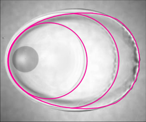
Figure 2. In the following, the experimental images corresponding to the deformed drops will be presented with a vertical orientation and then the sketch included in figure 1(c) represents a  $\unicode[STIX]{x03C0}/2$ radians clockwise rotation of the experimental visualizations. The experimental measurements of
  $s(\unicode[STIX]{x1D703},t)$ to be presented next, represent the distance of the outer perimeter of the drop measured from the origin of the moving frame of reference. The continuous lines in this figure represent the results of the detection algorithm included in the Matlab toolbox. The distances to the impact point,
  $\ell (\unicode[STIX]{x03C0}/2,t)$ and
  $\ell (3\unicode[STIX]{x03C0}/2,t)$, corresponding to the rim portions respectively located at
  $\unicode[STIX]{x03C0}/2$ and
  $3\unicode[STIX]{x03C0}/2$ (see also figure 1c), as well as the definition of the drop width,
  $w(t)$, are indicated in the figure to highlight the fact that the asymmetric shape of the drop can be characterized by two different length scales, namely
  $w(t)$ and
  $(\ell (\unicode[STIX]{x03C0}/2,t)+\ell (3\unicode[STIX]{x03C0}/2,t))/2$. Note that capital letters are used to denote dimensional quantities in order to differentiate them from their dimensionless versions, written using lower case letters. Then,
  $W=Rw$,
  $L=R\ell$,
  $T=R/(V\cos \unicode[STIX]{x1D712})t$. Here,
  $\unicode[STIX]{x1D712}=45^{\circ }$,
  $R=1.48\times 10^{-3}~\text{m}$ and
  $Oh=3.1\times 10^{-3}$,
  $V_{n}=V\cos \unicode[STIX]{x1D712}=1.73~\text{m}~\text{s}^{-1}$,
  $V_{t}=V_{n}\tan \unicode[STIX]{x1D712}=1.73~\text{m}~\text{s}^{-1}$ and
  $We=61$. The instants of time in the sequence are
  $T_{1}=0.85\times 10^{-3}~\text{s}$,
  $T_{2}=2.58\times 10^{-3}~\text{s}$,
  $T_{3}=4.30\times 10^{-3}~\text{s}$, which correspond to the following values of the dimensionless times:
  $t_{1}=T_{1}V_{n}/R=1$,
  $t_{2}=T_{2}V_{n}/R=3$,
  $t_{3}=T_{3}V_{n}/R=5$. Values of
  $t\pm 0.04$.
However, for clarity reasons, the theoretical shapes of the drops will not be represented in the moving frame of reference, but in the laboratory frame of reference in order to compare with the experimental visualizations like the ones depicted in figure 2, which will always be oriented vertically, in contrast with the sketch in figure 1(c), rotated  $\unicode[STIX]{x03C0}/2$ radians clockwise. In order to fix ideas, figures 1(c) and 2 also represent the impact point, which is the point at which the drop first touches the substrate and it is a fixed point in the laboratory frame of reference. Figure 2 also shows the origin of the moving frame of reference, which translates with a tangential velocity
  $V\sin \unicode[STIX]{x1D712}$ – or
  $\tan \unicode[STIX]{x1D712}$ in dimensionless form – with respect to the impact point. The origin of the moving frame of reference is the origin of radial distances and
  $\unicode[STIX]{x1D703}$ is measured counterclockwise with respect to the horizontal direction, which is the line contained in the plane of the substrate perpendicular to the plane of symmetry of the drop.
The theoretical results to be presented here could be used to describe most of the practical situations related to the spreading of drops of low viscosity liquids such as water or ethanol. Indeed, we will assume that the ranges of values of the dimensionless parameters defined in (2.1) are such that  $Oh\ll 1$,
  $We\gtrsim 10$,
  $Re\gtrsim 100$,
  $Fr\gtrsim 30$ a fact implying that the drop is noticeably deformed after impact – see figure 2 – and that viscous effects are confined within a narrow boundary layer. Moreover, it is also assumed that the diameters of the drops are in the range of a few millimetres or below, a fact implying that
  $Bo=\unicode[STIX]{x1D70C}gR^{2}/\unicode[STIX]{x1D70E}\lesssim O(1)$. However, capillary forces are much larger than the weight of the rim bordering the expanding liquid sheet, i.e.
  $b^{2}Bo=\unicode[STIX]{x1D70C}gR^{2}b^{2}/\unicode[STIX]{x1D70E}\ll 1$, with
  $b\ll 1$ the dimensionless rim thickness (see figures 1 and 2) and since, in addition,
  $Fr^{-1}=gR/V_{n}^{2}\ll 1$, namely that gravity does not have the time to sufficiently modify the initial drop velocity during the characteristic time the drop impacts the substrate, gravitational effects will be neglected in the analysis that follows.
Since the analysis will be carried out following the notation in Gordillo et al. (Reference Gordillo, Riboux and Quintero2019), from now on, lower case variables will be used to denote the dimensionless version of dimensional quantities, which will be written using capital letters. The origin of times is set at the instant the drop first touches the substrate at the so-called impact point (see figures 1c and 2).
In order to describe the time evolution of the rim position and thickness, it will prove essential to use the ideas in Gordillo et al. (Reference Gordillo, Riboux and Quintero2019) and divide the flow into the following well defined regions (see figure 1): (i) the drop region, where the liquid is accelerated thanks to pressure gradients and extends from  $r=0$ to
  $r=\sqrt{3t}$; (ii) the lamella, which is a slender region where the pressure gradient can be neglected and connects the end of the drop region, located at
  $r=\sqrt{3t}$, with the third region, the rim; (iii) the rim, which is located at a distance from the origin of the moving frame of reference
  $r=s(\unicode[STIX]{x1D703},t)$ and denotes the portion of fluid of thickness
  $b(\unicode[STIX]{x1D703},t)$ and velocity
  $v(\unicode[STIX]{x1D703},t)$ that limits the perimeter of the spreading drop.
Both the radial position and thickness of the rim can be calculated in the moving frame of reference by making use of the balances of mass and momentum (Taylor Reference Taylor1959; Eggers et al. Reference Eggers, Fontelos, Josserand and Zaleski2010; Villermaux & Bossa Reference Villermaux and Bossa2011; Gordillo et al. Reference Gordillo, Riboux and Quintero2019), i.e.
 $$\begin{eqnarray}\left.\begin{array}{@{}c@{}}\unicode[STIX]{x1D6FC}{\displaystyle \frac{\unicode[STIX]{x03C0}}{4}}{\displaystyle \frac{\text{d}b^{2}}{\text{d}t}}=[u(s,\unicode[STIX]{x1D703},t)-v]h(s,\unicode[STIX]{x1D703},t),\quad {\displaystyle \frac{\text{d}s}{\text{d}t}}=v,\\ \unicode[STIX]{x1D6FC}{\displaystyle \frac{\unicode[STIX]{x03C0}b^{2}}{4}}{\displaystyle \frac{\text{d}v}{\text{d}t}}=[u(s,\unicode[STIX]{x1D703},t)-v]^{2}h(s,\unicode[STIX]{x1D703},t)-(1+\unicode[STIX]{x1D6FD})\mathit{We}^{-1}-\unicode[STIX]{x1D6FE}We^{-1}Ca(v-\tan \unicode[STIX]{x1D712}\sin \unicode[STIX]{x1D703}),\end{array}\right\}\end{eqnarray}$$
 with  $u(s,\unicode[STIX]{x1D703},t)$ and
  $h(s,\unicode[STIX]{x1D703},t)$ in (2.2) the averaged radial velocity and the thickness of the thin film – the lamella – which, as it was mentioned above, extends along the spatio-temporal region
  $\sqrt{3t}\leqslant r\leqslant s(\unicode[STIX]{x1D703},t)$ (see figure 1). In (2.2),
  $\unicode[STIX]{x1D6FC}$ and
  $\unicode[STIX]{x1D6FD}$ depend on the wetting properties of the solid and, for the case at hand, which corresponds to hydrophilic substrates,
  $\unicode[STIX]{x1D6FC}=1/2$ and
  $\unicode[STIX]{x1D6FD}=0$ because the rim cross-sectional area will be approximated by that of a semicircle and the value of the advancing contact angle is assumed to be constant and equal to
  $\unicode[STIX]{x03C0}/2$. The last term in the momentum equation in (2.2), which represents the integral of the viscous shear forces at the wall
  ${\sim}Re^{-1}(v-\tan \unicode[STIX]{x1D712}\sin \unicode[STIX]{x1D703})/b$ along the rim region of width
  ${\sim}b$, with
  $\unicode[STIX]{x1D6FE}\sim O(1)$, will be neglected in what follows because the range of parameters investigated here is such that
  $Ca\ll 1$.
The system of (2.2) is integrated specifying the initial conditions at the instant  $t_{e}$ the lamella is initially ejected. In Riboux & Gordillo (Reference Riboux and Gordillo2014, Reference Riboux and Gordillo2017) it is predicted and verified experimentally that the ejection time can be expressed as
  $t_{e}=1.05\,\mathit{We}^{-2/3}$ and also that
 $$\begin{eqnarray}s(t_{e})=\sqrt{3t_{e}},\quad v(t_{e})=1/2\sqrt{3/t_{e}}\quad \text{and}\quad b(t_{e})={\displaystyle \frac{\sqrt{12}}{\unicode[STIX]{x03C0}}}t_{e}^{3/2}\end{eqnarray}$$
 if  $\mathit{Re}^{1/6}\mathit{Oh}^{2/3}<0.25$, which is the case for the experiments reported here and also for many other usual experimental conditions.
Clearly, the system (2.2) can only be integrated once the functions  $u(r,\unicode[STIX]{x1D703},t)$ and
  $h(r,\unicode[STIX]{x1D703},t)$ describing the averaged velocity and height of the lamella are particularized at the radial position where the rim is located, namely
  $r=s(\unicode[STIX]{x1D703},t)$. Applying local balances of mass and momentum in a differential portion of the lamella, it is shown in appendix A, that
  $u$ and
  $h$ satisfy the system of equations
 $$\begin{eqnarray}\left.\begin{array}{@{}c@{}}{\displaystyle \frac{\unicode[STIX]{x2202}(rh)}{\unicode[STIX]{x2202}t}}+u{\displaystyle \frac{\unicode[STIX]{x2202}(rh)}{\unicode[STIX]{x2202}r}}+rh{\displaystyle \frac{\unicode[STIX]{x2202}u}{\unicode[STIX]{x2202}r}}=\tan \unicode[STIX]{x1D712}\sin \unicode[STIX]{x1D703}{\displaystyle \frac{\unicode[STIX]{x1D6FF}}{2}},\\ {\displaystyle \frac{\unicode[STIX]{x2202}u}{\unicode[STIX]{x2202}t}}+u{\displaystyle \frac{\unicode[STIX]{x2202}u}{\unicode[STIX]{x2202}r}}=-\unicode[STIX]{x1D706}{\displaystyle \frac{u}{h\sqrt{\mathit{Re }t}}},\end{array}\right\}\end{eqnarray}$$
with the friction factor given by
 $$\begin{eqnarray}\unicode[STIX]{x1D706}(r,\unicode[STIX]{x1D703},t)\simeq 1-\tan \unicode[STIX]{x1D712}\sin \unicode[STIX]{x1D703}\sqrt{{\displaystyle \frac{x}{3}}}+{\displaystyle \frac{\tan ^{2}\unicode[STIX]{x1D712}\cos ^{2}\unicode[STIX]{x1D703}}{18}}x\quad \text{where }x=3\left({\displaystyle \frac{t}{r}}\right)^{2}\end{eqnarray}$$
and
 $$\begin{eqnarray}\unicode[STIX]{x1D6FF}=\sqrt{{\displaystyle \frac{t}{Re}}}\end{eqnarray}$$
 indicating the boundary layer thickness which, in a first approximation, does not depend on either  $r$ or
  $\unicode[STIX]{x1D703}$, as it is demonstrated in appendix B.
The partial differential equations (2.4) can be approximately solved, in the limit  $Re\gg 1$, expressing
  $u$ and
  $h$ as (Gordillo et al. Reference Gordillo, Riboux and Quintero2019)
 $$\begin{eqnarray}\left.\begin{array}{@{}c@{}}u(r,\unicode[STIX]{x1D703},t)=u_{0}(r,t)+\mathit{Re}^{-1/2}u_{1}(r,\unicode[STIX]{x1D703},t)+O(\mathit{Re}^{-1}),\\ h(r,\unicode[STIX]{x1D703},t)=h_{0}(r,t)+\mathit{Re}^{-1/2}h_{1}(r,\unicode[STIX]{x1D703},t)+O(\mathit{Re}^{-1}).\end{array}\right\}\end{eqnarray}$$
 The substitution of the ansatz (2.7) into the system (2.4), yields the following four partial differential equations for  $u_{0}(r,t)$,
  $h_{0}(r,t)$,
  $u_{1}(r,\unicode[STIX]{x1D703},t)$ and
  $h_{1}(r,\unicode[STIX]{x1D703},t)$:
 $$\begin{eqnarray}\left.\begin{array}{@{}c@{}}{\displaystyle \frac{\unicode[STIX]{x2202}u_{0}}{\unicode[STIX]{x2202}t}}+u_{0}{\displaystyle \frac{\unicode[STIX]{x2202}u_{0}}{\unicode[STIX]{x2202}r}}=0\quad \;\Longrightarrow \;\quad {\displaystyle \frac{\text{D}u_{0}}{\text{D}t}}=0,\\ {\displaystyle \frac{\unicode[STIX]{x2202}(rh_{0})}{\unicode[STIX]{x2202}t}}+u_{0}{\displaystyle \frac{\unicode[STIX]{x2202}(rh_{0})}{\unicode[STIX]{x2202}r}}+rh_{0}{\displaystyle \frac{\unicode[STIX]{x2202}u_{0}}{\unicode[STIX]{x2202}r}}=0\quad \;\Longrightarrow \;\quad {\displaystyle \frac{\text{D}(rh_{0})}{\text{D}t}}=-rh_{0}{\displaystyle \frac{\unicode[STIX]{x2202}u_{0}}{\unicode[STIX]{x2202}r}},\end{array}\right\}\end{eqnarray}$$
 $$\begin{eqnarray}\left.\begin{array}{@{}c@{}}{\displaystyle \frac{\unicode[STIX]{x2202}u_{1}}{\unicode[STIX]{x2202}t}}+u_{0}{\displaystyle \frac{\unicode[STIX]{x2202}u_{1}}{\unicode[STIX]{x2202}r}}+u_{1}{\displaystyle \frac{\unicode[STIX]{x2202}u_{0}}{\unicode[STIX]{x2202}r}}=-{\displaystyle \frac{\unicode[STIX]{x1D706}u_{0}}{h_{0}\sqrt{t}}}\quad \;\Longrightarrow \;\quad {\displaystyle \frac{\text{D}u_{1}}{\text{D}t}}+u_{1}{\displaystyle \frac{\unicode[STIX]{x2202}u_{0}}{\unicode[STIX]{x2202}r}}=-{\displaystyle \frac{\unicode[STIX]{x1D706}u_{0}}{h_{0}\sqrt{t}}},\\ {\displaystyle \frac{\unicode[STIX]{x2202}(rh_{1})}{\unicode[STIX]{x2202}t}}+u_{0}{\displaystyle \frac{\unicode[STIX]{x2202}(rh_{1})}{\unicode[STIX]{x2202}r}}+u_{1}{\displaystyle \frac{\unicode[STIX]{x2202}(rh_{0})}{\unicode[STIX]{x2202}r}}+rh_{0}{\displaystyle \frac{\unicode[STIX]{x2202}u_{1}}{\unicode[STIX]{x2202}r}}+rh_{1}{\displaystyle \frac{\unicode[STIX]{x2202}u_{0}}{\unicode[STIX]{x2202}r}}-\tan \unicode[STIX]{x1D712}\sin \unicode[STIX]{x1D703}{\displaystyle \frac{\sqrt{t}}{2}}=0\\ \;\Longrightarrow \;\quad {\displaystyle \frac{\text{D}(rh_{1})}{\text{D}t}}+rh_{1}{\displaystyle \frac{\unicode[STIX]{x2202}u_{0}}{\unicode[STIX]{x2202}r}}=\tan \unicode[STIX]{x1D712}\sin \unicode[STIX]{x1D703}{\displaystyle \frac{\sqrt{t}}{2}}-{\displaystyle \frac{\unicode[STIX]{x2202}}{\unicode[STIX]{x2202}r}}(u_{1}rh_{0}).\end{array}\right\}\end{eqnarray}$$
 Here  $\text{D}/\text{D}t\equiv \unicode[STIX]{x2202}/\unicode[STIX]{x2202}t+u_{0}\unicode[STIX]{x2202}/\unicode[STIX]{x2202}r$.
Equations (2.8)–(2.9) will be solved using the method of characteristics, as we already did in Gordillo et al. (Reference Gordillo, Riboux and Quintero2019) for the case of normal impact ( $\unicode[STIX]{x1D712}=0$), once appropriate boundary conditions are imposed at the spatio-temporal boundary
  $(r,t)=(\sqrt{3x},x)$ separating the drop and the lamella regions. For that purpose, note that at the spatio-temporal boundary
  $r=\sqrt{3x}$ both the height of the lamella and the liquid velocity were deduced in the potential flow limit (frictionless limit) in Riboux & Gordillo (Reference Riboux and Gordillo2014, Reference Riboux and Gordillo2016):
  $u(\sqrt{3x})=u_{a}(x)=\sqrt{3/x}$ and
  $h(\sqrt{3x},x)=h_{a}(x)$, with
  $h_{a}(x)$ a function determined numerically in Riboux & Gordillo (Reference Riboux and Gordillo2016), which can be approximated as (Gordillo et al. Reference Gordillo, Riboux and Quintero2019)
 $$\begin{eqnarray}\displaystyle h_{a}(x)=P(x) & = & \displaystyle \mathop{\sum }_{i=0}^{9}p_{i}x^{i}\nonumber\\ \displaystyle & & \displaystyle \text{with}\quad p_{0}=3.95812707\times 10^{-4},\quad p_{1}=1.22669850\times 10^{-1},\nonumber\\ \displaystyle & & \displaystyle p_{2}=-1.04054024\times 10^{-1},\quad p_{3}=4.37229580\times 10^{-2},\nonumber\\ \displaystyle & & \displaystyle p_{4}=-1.09184802\times 10^{-2},\quad p_{5}=1.70579418\times 10^{-3},\nonumber\\ \displaystyle & & \displaystyle p_{6}=-1.67926979\times 10^{-4},\quad p_{7}=1.01063551\times 10^{-5},\nonumber\\ \displaystyle & & \displaystyle p_{8}=-3.39290090\times 10^{-7}\quad p_{9}=4.86535897\times 10^{-9}.\end{eqnarray}$$
 The presence of the boundary layer does not change, to leading order, the normal velocity field at the surface of the drop with respect to the potential flow solution. Therefore, the mass balance demands that the mass flux per unit length at  $r=\sqrt{3x}$ in a real case, namely when a boundary layer is present, is identical to this quantity in the frictionless limit. Hence, (Gordillo et al. Reference Gordillo, Riboux and Quintero2019)
 $$\begin{eqnarray}h_{a}(x)u_{a}(x)=u_{a}(h-\unicode[STIX]{x1D6FF})+{\displaystyle \frac{\unicode[STIX]{x1D6FF}}{2}}(u_{a}+\tan \unicode[STIX]{x1D712}\sin \unicode[STIX]{x1D703})=u(r=\sqrt{3x},\unicode[STIX]{x1D703},x)h(\sqrt{3x},\unicode[STIX]{x1D703},x),\end{eqnarray}$$
where we have assumed that the velocity profiles are linear within the boundary layer (see (A 5) in appendix A). Therefore, from the two equations in (2.11) it can be deduced that
 $$\begin{eqnarray}\left.\begin{array}{@{}c@{}}h(\sqrt{3x},\unicode[STIX]{x1D703},x)=h_{a}\left(1+{\displaystyle \frac{\unicode[STIX]{x1D6FF}}{2h_{a}}}\left(1-{\displaystyle \frac{\tan \unicode[STIX]{x1D712}\sin \unicode[STIX]{x1D703}}{u_{a}}}\right)\right),\\ u(\sqrt{3x},\unicode[STIX]{x1D703},x)=u_{a}\left(1+{\displaystyle \frac{\unicode[STIX]{x1D6FF}}{2h_{a}}}\left(1-{\displaystyle \frac{\tan \unicode[STIX]{x1D712}\sin \unicode[STIX]{x1D703}}{u_{a}}}\right)\right)^{-1},\end{array}\right\}\end{eqnarray}$$
 with  $u_{a}=\sqrt{3/x}$ and
  $\unicode[STIX]{x1D6FF}(x)=\sqrt{x/Re}$.
In the limit  $Re\gg 1$, (2.12) can be linearized to give
 $$\begin{eqnarray}\left.\begin{array}{@{}c@{}}h(\sqrt{3x},\unicode[STIX]{x1D703},x)=h_{a}(x)+{\displaystyle \frac{\sqrt{x}}{2}}\left(1-{\displaystyle \frac{\tan \unicode[STIX]{x1D712}\sin \unicode[STIX]{x1D703}}{\sqrt{3}}}\sqrt{x}\right)Re^{-1/2},\\ u(\sqrt{3x},\unicode[STIX]{x1D703},x)\simeq \sqrt{{\displaystyle \frac{3}{x}}}-{\displaystyle \frac{\sqrt{3}}{2h_{a}(x)}}\unicode[STIX]{x1D709}\left(1-{\displaystyle \frac{\tan \unicode[STIX]{x1D712}\sin \unicode[STIX]{x1D703}}{\sqrt{3}}}\sqrt{x}\right)Re^{-1/2},\end{array}\right\}\end{eqnarray}$$
 with  $\unicode[STIX]{x1D709}$ a variable such that the expression in (2.13) is a good approximation to the exact value of
  $u$ in (2.12) for all values of
  $x$. For instance, when
  $\unicode[STIX]{x1D6FF}\ll h_{a}$,
  $\unicode[STIX]{x1D709}=1$, while if
  $\unicode[STIX]{x1D6FF}\sim h_{a}$, the approximation in (2.13) to the exact value will be good if
  $\unicode[STIX]{x1D709}\simeq 2/3$. The range of Ohnesorge numbers considered here,
  $10^{-3}\leqslant Oh\leqslant 10^{-2}$, is such that the ratio
  $\unicode[STIX]{x1D6FF}/h_{a}$ is of order unity and, then, all the results presented here are calculated taking the value
  $\unicode[STIX]{x1D709}=2/3$ (Gordillo et al. Reference Gordillo, Riboux and Quintero2019).
Therefore, making use of (2.7) and (2.13) it can be deduced that
 $$\begin{eqnarray}\left.\begin{array}{@{}c@{}}u_{0}(\sqrt{3x},\unicode[STIX]{x1D703},x)=\sqrt{{\displaystyle \frac{3}{x}}},\quad u_{1}(\sqrt{3x},\unicode[STIX]{x1D703},x)=-{\displaystyle \frac{\sqrt{3}}{2h_{a}(x)}}\unicode[STIX]{x1D709}\left(1-{\displaystyle \frac{\tan \unicode[STIX]{x1D712}\sin \unicode[STIX]{x1D703}}{\sqrt{3}}}\sqrt{x}\right),\\ h_{0}(\sqrt{3x},\unicode[STIX]{x1D703},x)=h_{a}(x)\quad \text{and}\quad h_{1}(\sqrt{3x},\unicode[STIX]{x1D703},x)={\displaystyle \frac{\sqrt{x}}{2}}\left(1-{\displaystyle \frac{\tan \unicode[STIX]{x1D712}\sin \unicode[STIX]{x1D703}}{\sqrt{3}}}\sqrt{x}\right).\end{array}\right\}\end{eqnarray}$$
 We now follow the steps in Gordillo et al. (Reference Gordillo, Riboux and Quintero2019) and integrate the momentum equation in (2.8) along rays  $\text{d}r/\text{d}t=\sqrt{3/x}$ subjected to the corresponding boundary condition in (2.14), yielding
 $$\begin{eqnarray}\left.\begin{array}{@{}c@{}}u_{0}(r,t)=\sqrt{{\displaystyle \frac{3}{x}}}\quad \text{along}\quad {\displaystyle \frac{\text{d}r}{\text{d}t}}=\sqrt{{\displaystyle \frac{3}{x}}}\quad \;\Longrightarrow \;\quad r=\sqrt{3x}+\sqrt{{\displaystyle \frac{3}{x}}}(t-x)\\ \;\Longrightarrow \;\quad r=\sqrt{{\displaystyle \frac{3}{x}}}t\quad \;\Longrightarrow \;x=3\left({\displaystyle \frac{t}{r}}\right)^{2}\quad \;\Longrightarrow \;\quad u_{0}(r,t)=\sqrt{{\displaystyle \frac{3}{3(t/r)^{2}}}}={\displaystyle \frac{r}{t}}.\end{array}\right\}\end{eqnarray}$$
 Moreover, the integration of the equation for  $h_{0}(r,t)$ in (2.8) along the ray
  $\text{d}r/\text{d}t=\sqrt{3/x}$ yields
 $$\begin{eqnarray}{\displaystyle \frac{\unicode[STIX]{x2202}(rh_{0})}{\unicode[STIX]{x2202}t}}+u_{0}{\displaystyle \frac{\unicode[STIX]{x2202}(rh_{0})}{\unicode[STIX]{x2202}r}}+{\displaystyle \frac{rh_{0}}{t}}=0\quad \;\Longrightarrow \;\quad {\displaystyle \frac{\text{D}(rh_{0}t)}{\text{D}t}}=0\quad \;\Longrightarrow \;\quad h_{0}(r,t)=9{\displaystyle \frac{t^{2}}{r^{4}}}h_{a}[3(t/r)^{2}],\end{eqnarray}$$
 where we have made use of the fact that  $\unicode[STIX]{x2202}u_{0}/\unicode[STIX]{x2202}r=1/t$, the relationship between
  $x$ with
  $r$ and
  $t$ in (2.15) and of the corresponding boundary condition in (2.14). Equations (2.15)–(2.16) recovers the result in Gordillo et al. (Reference Gordillo, Riboux and Quintero2019).
Now, using the expression for  $u_{0}$ in (2.15) and multiplying both sides of the equations in (2.9) by
  $t$, we find that
 $$\begin{eqnarray}{\displaystyle \frac{\text{D}(u_{1}t)}{\text{D}t}}=-{\displaystyle \frac{\unicode[STIX]{x1D706}u_{0}}{h_{0}\sqrt{t}}}t,\quad {\displaystyle \frac{\text{D}(rh_{1}t)}{\text{D}t}}=-{\displaystyle \frac{1}{t}}{\displaystyle \frac{\unicode[STIX]{x2202}}{\unicode[STIX]{x2202}r}}(rh_{0}tu_{1}t)+\tan \unicode[STIX]{x1D712}\sin \unicode[STIX]{x1D703}{\displaystyle \frac{t^{3/2}}{2}}.\end{eqnarray}$$
 The equation for  $u_{1}$ in (2.17) can be integrated along rays
  $r=\sqrt{3/x}\,t$ taking into account that, by virtue of (2.16),
  $\text{D}(rh_{0}t)/\text{D}t=0$,
 $$\begin{eqnarray}\left.\begin{array}{@{}c@{}}{\displaystyle \frac{\text{D}(u_{1}t)}{\text{D}t}}=-{\displaystyle \frac{\unicode[STIX]{x1D706}u_{0}}{h_{0}\sqrt{t}}}t\quad \;\Longrightarrow \;\quad {\displaystyle \frac{\text{D}(u_{1}trh_{0}t)}{\text{D}t}}={\displaystyle \frac{-3\unicode[STIX]{x1D706}}{x}}t^{5/2}\quad \;\Longrightarrow \;\\ u_{1}(r,\unicode[STIX]{x1D703},t)=-{\displaystyle \frac{1}{th_{a}(x)}}\left[{\displaystyle \frac{\sqrt{3}x}{2}}\unicode[STIX]{x1D709}\left(1-{\displaystyle \frac{\tan \unicode[STIX]{x1D712}\sin \unicode[STIX]{x1D703}}{\sqrt{3}}}\sqrt{x}\right)+{\displaystyle \frac{2\sqrt{3}\unicode[STIX]{x1D706}}{7x^{5/2}}}(t^{7/2}-x^{7/2})\right],\end{array}\right\}\end{eqnarray}$$
 where we made use of the boundary condition for  $u_{1}$ in (2.14) and also of the fact that, along rays
  $\text{d}r/\text{d}t=u_{0}=\sqrt{3/x}$ departing from the spatio-temporal boundary
  $(r,t)=(\sqrt{3x},x)$,
  $r=\sqrt{3/x}t$,
  $u_{0}=\sqrt{3/x}$ and
  $rh_{0}t=\sqrt{3x}h_{a}(x)x$.
To integrate the equation for  $h_{1}$ in (2.17) we make use of our previous ideas in Gordillo et al. (Reference Gordillo, Riboux and Quintero2019), which we reproduce here for clarity purposes, and note that
  $\unicode[STIX]{x2202}(u_{1}trh_{0}t)/\unicode[STIX]{x2202}r$ can be calculated as the increment
  $\text{d}(u_{1}trh_{0}t)$ between two neighbouring rays departing from the spatio-temporal boundary
  $(r,t)=(\sqrt{3x},x)$ at the consecutive instants
  $x-\text{d}x$ and
  $x$ which, at a given instant
  $t$ are thus separated by a distance
  $\text{d}r=\sqrt{3}/2x^{-3/2}t\,\text{d}x$. Consequently, making use of the solution for
  $u_{1}trh_{0}t$ in (2.18) and of the boundary condition for
  $u_{1}$ in (2.14),
 $$\begin{eqnarray}\left.\begin{array}{@{}c@{}}rh_{0}tu_{1}t-(rh_{0}tu_{1}t)(x)=-{\displaystyle \frac{6\unicode[STIX]{x1D706}}{7x}}(t^{7/2}-x^{7/2})\quad \text{with}\\ (rh_{0}tu_{1}t)(x)=-{\displaystyle \frac{\sqrt{3}}{2}}\unicode[STIX]{x1D709}\left(1-{\displaystyle \frac{\tan \unicode[STIX]{x1D712}\sin \unicode[STIX]{x1D703}}{\sqrt{3}}}\sqrt{x}\right)x^{2}\sqrt{3x}\end{array}\right\}\end{eqnarray}$$
 and taking into account that  $\text{d}r=\sqrt{3}/2x^{-3/2}t\,\text{d}x$,
 $$\begin{eqnarray}-{\displaystyle \frac{1}{t}}{\displaystyle \frac{\unicode[STIX]{x2202}}{\unicode[STIX]{x2202}r}}(u_{1}trh_{0}t)={\displaystyle \frac{2x^{3/2}}{\sqrt{3}}}{\displaystyle \frac{1}{t^{2}}}{\displaystyle \frac{\unicode[STIX]{x2202}}{\unicode[STIX]{x2202}x}}(rh_{0}tu_{1}t(x))-{\displaystyle \frac{12x^{3/2}}{7\sqrt{3}}}{\displaystyle \frac{1}{t^{2}}}{\displaystyle \frac{\unicode[STIX]{x2202}}{\unicode[STIX]{x2202}x}}\left[{\displaystyle \frac{\unicode[STIX]{x1D706}}{x}}(t^{7/2}-x^{7/2})\right].\end{eqnarray}$$
Hence,
 $$\begin{eqnarray}\displaystyle -{\displaystyle \frac{1}{t}}{\displaystyle \frac{\unicode[STIX]{x2202}}{\unicode[STIX]{x2202}r}}(u_{1}trh_{0}t) & = & \displaystyle -{\displaystyle \frac{2}{14\sqrt{3}t^{2}}}\left[\left(52.5\unicode[STIX]{x1D709}\left(1-{\displaystyle \frac{\tan \unicode[STIX]{x1D712}\sin \unicode[STIX]{x1D703}}{\sqrt{3}}}\sqrt{x}\right)-30\unicode[STIX]{x1D706}\right)x^{3}-12\unicode[STIX]{x1D706}x^{-1/2}t^{7/2}\right]\nonumber\\ \displaystyle & & \displaystyle +\,{\displaystyle \frac{x^{4}}{2\sqrt{x}}}{\displaystyle \frac{\unicode[STIX]{x1D709}}{t^{2}}}\tan \unicode[STIX]{x1D712}\sin \unicode[STIX]{x1D703}-{\displaystyle \frac{12x^{3/2}}{7\sqrt{3}}}{\displaystyle \frac{1}{xt^{2}}}(t^{7/2}-x^{7/2}){\displaystyle \frac{\unicode[STIX]{x2202}\unicode[STIX]{x1D706}}{\unicode[STIX]{x2202}x}},\end{eqnarray}$$
with
 $$\begin{eqnarray}{\displaystyle \frac{\unicode[STIX]{x2202}\unicode[STIX]{x1D706}}{\unicode[STIX]{x2202}x}}={\displaystyle \frac{1}{2}}\left(-{\displaystyle \frac{\tan \unicode[STIX]{x1D712}\sin \unicode[STIX]{x1D703}}{\sqrt{3x}}}+{\displaystyle \frac{\tan ^{2}\unicode[STIX]{x1D712}\cos ^{2}\unicode[STIX]{x1D703}}{9}}\right)\end{eqnarray}$$
 and where use of the boundary condition for  $u_{1}$ in (2.14) has been made.
The substitution of (2.21)–(2.22) into (2.17) and the integration of the resulting equation for  $h_{1}$ along the ray
  $\text{d}r/\text{d}t=\sqrt{3/x}$ yields an expression that, once it is inserted into the ansatz (2.7), yields the following expressions for
  $u(r,\unicode[STIX]{x1D703},t)$ and
  $h(r,\unicode[STIX]{x1D703},t)$:
 $$\begin{eqnarray}\left.\begin{array}{@{}c@{}}u(r,\unicode[STIX]{x1D703},t)={\displaystyle \frac{r}{t}}-{\displaystyle \frac{\mathit{Re}^{-1/2}}{t}}\left[{\displaystyle \frac{\sqrt{3}x}{2h_{a}(x)}}\unicode[STIX]{x1D709}\left(1-{\displaystyle \frac{\tan \unicode[STIX]{x1D712}\sin \unicode[STIX]{x1D703}}{\sqrt{3}}}\sqrt{x}\right)\right.\\ +\left.{\displaystyle \frac{2\sqrt{3}\unicode[STIX]{x1D706}}{7h_{a}(x)x^{5/2}}}(t^{7/2}-x^{7/2})\right],\\ h(r,\unicode[STIX]{x1D703},t)=9{\displaystyle \frac{t^{2}}{r^{4}}}h_{a}[3(t/r)^{2}]+{\displaystyle \frac{Re^{-1/2}}{rt}}\left[{\displaystyle \frac{\sqrt{3}}{2}}x^{2}\left(1-{\displaystyle \frac{\tan \unicode[STIX]{x1D712}\sin \unicode[STIX]{x1D703}}{\sqrt{3}}}\sqrt{x}\right)\right.\\ +\left.{\displaystyle \frac{1}{5}}\tan \unicode[STIX]{x1D712}\sin \unicode[STIX]{x1D703}(t^{5/2}-x^{5/2})\right.\\ +{\displaystyle \frac{\sqrt{3}}{42}}\left(105\unicode[STIX]{x1D709}\left(1-{\displaystyle \frac{\tan \unicode[STIX]{x1D712}\sin \unicode[STIX]{x1D703}}{\sqrt{3}}}\sqrt{x}\right)-60\unicode[STIX]{x1D706}\right)x^{3}(t^{-1}-x^{-1})+{\displaystyle \frac{24\sqrt{3}\unicode[STIX]{x1D706}}{105}}x^{-1/2}(t^{5/2}-x^{5/2})\\ \left.-x^{4}(t^{-1}-x^{-1})\left({\displaystyle \frac{\tan \unicode[STIX]{x1D712}\sin \unicode[STIX]{x1D703}}{2\sqrt{x}}}\unicode[STIX]{x1D709}+{\displaystyle \frac{6}{7\sqrt{3}}}\left(-{\displaystyle \frac{\tan \unicode[STIX]{x1D712}\sin \unicode[STIX]{x1D703}}{\sqrt{3x}}}+{\displaystyle \frac{\tan ^{2}\unicode[STIX]{x1D712}\cos ^{2}\unicode[STIX]{x1D703}}{9}}\right)\right)\right.\\ \left.-{\displaystyle \frac{12x^{1/2}}{35\sqrt{3}}}\left(-{\displaystyle \frac{\tan \unicode[STIX]{x1D712}\sin \unicode[STIX]{x1D703}}{\sqrt{3x}}}+{\displaystyle \frac{\tan ^{2}\unicode[STIX]{x1D712}\cos ^{2}\unicode[STIX]{x1D703}}{9}}\right)(t^{5/2}-x^{5/2})\vphantom{{\displaystyle \frac{\sqrt{3}}{2}}}\right].\end{array}\right\}\end{eqnarray}$$
Here we have also made use of (2.15), (2.16) and (2.18).
As expected, (2.23) recovers, in the limit  $\unicode[STIX]{x1D712}=0$, the equations for
  $u$ and
  $h$ deduced in Gordillo et al. (Reference Gordillo, Riboux and Quintero2019) to describe the spreading of drops impacting perpendicularly over a smooth dry substrate. In addition, the expressions for
  $u$ and
  $h$ in (2.23) particularized at
  $\unicode[STIX]{x1D703}=0$ are, except for the terms proportional to
  $Re^{-1/2}\tan ^{2}\unicode[STIX]{x1D712}\cos ^{2}\unicode[STIX]{x1D703}$, identical to those deduced in Gordillo et al. (Reference Gordillo, Riboux and Quintero2019), as the interested reader could check. It will be shown in § 4, where we discuss the final shapes of the deformed drops, that the prefactors of the additional terms in (2.23) affecting
  $\tan ^{2}\unicode[STIX]{x1D712}\cos ^{2}\unicode[STIX]{x1D703}$ are comparatively small when compared with a similar order of magnitude terms. As it will become clear in § 4, this is the reason why the experimental fittings describing the axisymmetric spreading of drops can be used to predict the maximum width of the spreading drop when the Reynolds and Weber numbers are defined using the normal component of the velocity. This theoretical result, which is deduced here in the moving frame of reference and is supported by the observations made in Sikalo & Ganic (Reference Sikalo and Ganic2005), Laan et al. (Reference Laan, de Bruin, Bartolo, Josserand and Bonn2014) as well as by the experiments presented below, cannot be extrapolated to the rest of the values of
  $\unicode[STIX]{x1D703}$. Indeed, from the expression of
  $u$ in (2.23), note that the mean velocity and, hence, the flux of momentum entering into the rim at
  $\unicode[STIX]{x1D703}=0$ is larger than the corresponding value at
  $\unicode[STIX]{x1D703}=3\unicode[STIX]{x03C0}/2$, but smaller than the value at
  $\unicode[STIX]{x1D703}=\unicode[STIX]{x03C0}/2$. This is a consequence of the fact that, in the moving frame of reference, the flow induced by the wall, which is confined within the boundary layer, is directed in the same direction as the velocity field in the potential flow region located outside the boundary layer for
  $\unicode[STIX]{x1D703}=\unicode[STIX]{x03C0}/2$, but it is in the opposite direction for
  $\unicode[STIX]{x1D703}=3\unicode[STIX]{x03C0}/2$ (see figure 16 in appendix A). This boundary layer effect induces an asymmetry in the drop expansion process which will be appreciated in the figures below. Another way of realizing that the viscous boundary layer induces asymmetries is that (2.23) would not depend on
  $\unicode[STIX]{x1D703}$ in the limit
  $Re\rightarrow \infty$, namely if the viscous effects could be neglected, as it would be the case of the impact of drops in the Leidenfrost regime. Hence, in the frictionless case considered in Riboux & Gordillo (Reference Riboux and Gordillo2016), if the contact line did not pin the substrate, the rim would be a circle of time-varying radius with a centre translating in the tangential direction to the substrate with a (dimensional) velocity
  $V\sin \unicode[STIX]{x1D712}$. But there is another important reason explaining the asymmetries depicted in the drop spreading process illustrated in figure 2, which is that the condition determining the pinning of the advancing contact line to the substrate depends on
  $\unicode[STIX]{x1D703}$. Indeed, the pinning condition used here, to be validated in what follows, simply expresses that the rim portion located at the angle
  $\unicode[STIX]{x1D703}$ will stick to the substrate and, therefore, will conserve in time its position in the laboratory frame of reference when the radial rim velocity with respect to the substrate is zero. This condition, which reads as
 $$\begin{eqnarray}v(\unicode[STIX]{x1D703},t_{pin}(\unicode[STIX]{x1D703}))=\tan \unicode[STIX]{x1D712}\sin \unicode[STIX]{x1D703},\end{eqnarray}$$
 with  $v$ the rim radial velocity calculated in the moving frame of reference using (2.2) and
  $t_{pin}$ the instant of time the rim pins the substrate, indicates that, for a given value of
  $\unicode[STIX]{x1D712}\neq 0$, the rim portion stopping first will be the one located at
  $\unicode[STIX]{x1D703}=\unicode[STIX]{x03C0}/2$ and the rim portion stopping last will be the one located at
  $\unicode[STIX]{x1D703}=3\unicode[STIX]{x03C0}/2$. Indeed, from (2.24) it can be inferred that the rim at
  $\unicode[STIX]{x1D703}=\unicode[STIX]{x03C0}/2$ will stop when
  $v>0$, namely when the rim is expanding outwards in the relative frame of reference, that the rim at
  $\unicode[STIX]{x1D703}=0$ will stop when
  $v=0$, namely when the rim radial velocity is zero, and also that the rim at
  $\unicode[STIX]{x1D703}=3\unicode[STIX]{x03C0}/2$ will stop when
  $v<0$, namely when the rim is contracting inwards in the relative frame of reference. Let us point out here that we will quantify the rim contraction process (i.e. when
  $v(\unicode[STIX]{x1D703},t)<0$) in a simplified manner. Indeed, when
  $v<0$, the thickness of the liquid film
  $h$ is a small quantity which can be estimated by taking the limit
  $Re\rightarrow \infty$ in the equation for
  $h$ in (2.23), i.e.
 $$\begin{eqnarray}h\sim 9{\displaystyle \frac{t^{2}}{r^{4}}}h_{a}[3(t/r)^{2}]={\displaystyle \frac{3x}{r^{2}}}h_{a}(x),\end{eqnarray}$$
 with  $x=3(t/r)^{2}\sim O(1)$ the instant of time at which fluid particles are ejected from the boundary separating the drop and rim regions, namely
  $r=\sqrt{3x}$. The values of
  $h_{a}(x)$ are approximately constant around its maximum value,
  ${\approx}0.05$, for
  $0.7\lesssim x\lesssim 2.5$, as it can be deduced using (2.10) or, alternatively, see Gordillo et al. (Reference Gordillo, Riboux and Quintero2019). Since the rim recedes in the moving frame of reference for instants of time such that the drop is around its maximum radial extension, which is such that
  $s^{\ast }(\unicode[STIX]{x1D703}=0)\gg 1$ for the range of Weber numbers of interest here, namely
  $We\gg 1$ (see, for instance, figure 2 or the figures to be shown in the next section), the height of the liquid film when the drop is reaching its maximum extension can be estimated as
 $$\begin{eqnarray}h\sim {\displaystyle \frac{3x}{s^{\ast 2}}}h_{a}(x)\ll 1,\end{eqnarray}$$
 because  $x\sim O(1)$,
  $h_{a}\ll 1$,
  $s^{\ast }(\unicode[STIX]{x1D703}=0)\gg 1$ and, to simplify the notation,
  $s^{\ast }=s^{\ast }(\unicode[STIX]{x1D703}=0)$. Now, note that the ratio
  $h/\unicode[STIX]{x1D6FF}$, with
  $\unicode[STIX]{x1D6FF}=\sqrt{t/Re}$ and
  $h$ given by expression (2.26), yields
 $$\begin{eqnarray}{\displaystyle \frac{h}{\unicode[STIX]{x1D6FF}}}\sim {\displaystyle \frac{3xh_{a}/s^{\ast 2}}{\sqrt{s^{\ast }/Re}}}\sim {\displaystyle \frac{3xWe^{1/4}Oh^{-1/2}h_{a}}{s^{\ast 5/2}}},\end{eqnarray}$$
 where we have taken into account the definition of  $x$, from which
  $\unicode[STIX]{x1D6FF}\simeq \sqrt{s^{\ast }/Re}$ because
  $x$ is of order unity and we have used the relation
  $We=Re^{2}Oh^{2}$. It will be shown in § 4 that the analytical expression of
  $s^{\ast }$ deduced here can be fitted, for the case of low viscosity liquids considered here, as
  $s^{\ast }\sim We^{1/4}$, as already noted by Clanet et al. (Reference Clanet, Béguin, Richard and Quéré2004) and, hence, (2.27) reads as
 $$\begin{eqnarray}{\displaystyle \frac{h}{\unicode[STIX]{x1D6FF}}}\sim {\displaystyle \frac{3xOh^{-1/2}h_{a}}{We^{3/8}}}\lesssim O(1),\end{eqnarray}$$
 because  $We\gg 1$,
  $x\sim O(1)$ and
  $Oh^{-1/2}h_{a}\simeq 1$ for the range of values of
  $Oh$ considered here (see table 1) since
  $h_{a}\lesssim 0.05$. Equation (2.28) expresses that viscous diffusion penetrates across the whole width of the lamella and, thus, the averaged liquid velocity at the entrance of the rim is noticeably smaller than the corresponding value of the potential flow limit
  $Re\rightarrow \infty$, as it can be also inferred using the equation for
  $u$ in (2.23).
Motivated by these reasons, the relative fluxes of mass  $(u-v)h$ and momentum
  $(u-v)^{2}h$ in (2.2) will be neglected here in the description of the rim contraction process. Then, in order to quantify the rim dynamics when
  $v(\unicode[STIX]{x1D703},t)<0$ in the moving frame of reference, equations (2.2) are integrated analytically from the instant
  $t^{\ast }(\unicode[STIX]{x1D703})$ at which the rim velocity is zero,
  $v(\unicode[STIX]{x1D703})=0$, which yields
 $$\begin{eqnarray}v={\displaystyle \frac{-4(1+\unicode[STIX]{x1D6FD})}{\unicode[STIX]{x1D6FC}We\unicode[STIX]{x03C0}b^{\ast 2}}}(t-t^{\ast })\quad \text{and}\quad s=s^{\ast }-{\displaystyle \frac{2(1+\unicode[STIX]{x1D6FD})}{\unicode[STIX]{x1D6FC}We\unicode[STIX]{x03C0}b^{\ast 2}}}(t-t^{\ast })^{2},\end{eqnarray}$$
 with  $s^{\ast }$ the value of
  $s(\unicode[STIX]{x1D703})$ at
  $t=t^{\ast }(\unicode[STIX]{x1D703})$ and
  $b^{\ast }$ the value of
  $b$ at
  $\unicode[STIX]{x1D703}=0$ at the instant
  $t=t^{\ast }(\unicode[STIX]{x1D703}=0)$. Note that, from now on, the superscript ‘
 $^{\ast }$’ will be used to indicate the values of variables when
  $v=0$ and the subscript ‘
 $pin$’ will be used to denote the value of a variable at the instant the rim pins the substrate, namely when its velocity is zero in the laboratory frame of reference. Let us also point out that, in the limit
  $\unicode[STIX]{x1D712}\ll 1$,
  $b^{\ast }(\unicode[STIX]{x1D703})=b^{\ast }(\unicode[STIX]{x1D703}=0)$ because the deformed drop is nearly axisymmetric, but we extend this result here for arbitrary values of
  $\unicode[STIX]{x1D712}$ because this additional approximation simplifies the algebra in § 4 and the agreement with experimental observations in §§ 3 and 4 will be shown to be good for low to moderate values of
  $\unicode[STIX]{x1D712}$.
Then, the theoretical curves in the comparisons with the experimental data to be shown in the next section are calculated as follows: for  $v(\unicode[STIX]{x1D703})>0$, namely when the rim portion located at
  $\unicode[STIX]{x1D703}$ is expanding outwards in the relative frame of reference, the system of ordinary differential equations (2.2) is integrated from the ejection time
  $t=t_{e}=1.05We^{-2/3}$ using (2.3) as initial conditions and using the analytical expressions of
  $u$ and
  $h$ given in (2.23). For
  $v(\unicode[STIX]{x1D703})<0$, namely when the rim portion located at
  $\unicode[STIX]{x1D703}$ is contracting inwards in the relative frame of reference, we make use of the analytical expressions in (2.29) using
  $b^{\ast }=b^{\ast }(\unicode[STIX]{x1D703}=0)$ and
  $s^{\ast }(\unicode[STIX]{x1D703})$ calculated by integrating the system (2.2) up to the instant
  $t^{\ast }(\unicode[STIX]{x1D703})$ for which
  $v(\unicode[STIX]{x1D703})=0$. The expansion (
 $v(\unicode[STIX]{x1D703},t)>0$) or contraction (
 $v(\unicode[STIX]{x1D703},t)<0$) processes for a given value of
  $\unicode[STIX]{x1D703}$ are not continued beyond the instant of time
  $t_{pin}(\unicode[STIX]{x1D703})$ at which condition (2.24) is satisfied; when this happens, the rim spatial position is then kept constant in the laboratory frame of reference.
Note that the results presented here for arbitrary values of  $\unicode[STIX]{x1D712}$ have been deduced neglecting fluxes and capillarity effects along the azimuthal direction. Thanks to this simplification, the temporal evolution of the rim located at a fixed value of
  $\unicode[STIX]{x1D703}$ can be straightforwardly calculated from
  $t=t_{e}=1.05We^{-2/3}$ – see (2.3) – up to the instant of time
  $t_{pin}(\unicode[STIX]{x1D703})$ when (2.24) is verified, by either integrating the system (2.2) using the analytical expressions for
  $u$ and
  $h$ given in (2.23) or using the analytical expressions given in (2.29). The validity of the simplified theoretical approach presented here, which does not resort on any adjustable constants, will be checked in what follows.
3 Experiments and comparison with theory
The sketch in figure 3 illustrates that the experimental images presented here have been recorded using a high-speed camera, Phantom V710, placed perpendicularly to two different types of smooth and dry glass slides, which are replaced after each experiment. The high-speed camera is operated, except for one case indicated in figure 4, at 33009 f.p.s. (frames per second), obtaining a spatial resolution of  $45~\unicode[STIX]{x03BC}\text{m}$ per pixel. The glass slides can be inclined with respect to the horizontal direction at an angle
  $\unicode[STIX]{x1D712}$ which is measured and fixed to
  $\unicode[STIX]{x1D712}=15^{\circ }$,
  $30^{\circ }$,
  $45^{\circ }$ or
  $\unicode[STIX]{x1D712}=60^{\circ }$ thanks to the use of an adjustable mounting plate (see figure 3). Drops of two liquids, water and ethanol, are formed quasi-statically from a needle which can be placed at a variable height from the impacting surface in order to modify the impact velocity
  $V$ of the falling drops. In table 1 we provide the experimental values of
  $We$,
$We$,  $Re$,
$Re$,  $Oh$,
$Oh$,  $Fr$,
$Fr$,  $Bo$ and
  $\unicode[STIX]{x1D712}$ explored in this study, as well as the range of values of the static contact angles. Additional experimental information is provided in appendix D.

Figure 3. ( $A$) The experimental images presented in the main text have been obtained by means of the part of the set-up represented in (
 $B$), which consists of an AP180/M Thorlabs adjustable angle mounting plate (
 $a$), fixed to a horizontal non-vibrating Photon Control table (
 $b$) thanks to a right-angle plate Thorlabs AP90 (
 $c$). A diffusor light Thorlabs DG100
 $\times$100 (
 $d$) is fixed to the AP180/M Thorlabs adjustable angle mounting plate and placed perpendicularly to a Phantom camera V710 coupled with a Sigma 105 mm DG Macro objective (
 $e$). Glass slides, either Knittel or Labbox,
  $76\times 26~\text{mm}$, (
 $f$) are placed on the diffusor and are fixed thanks to the stackable filter holder Thorlabs FH2D. The glass slides are removed and replaced after each experiment. A tripod Manfrotto model #028 (
 $g$) is used to move vertically along the
  $y$-axis and to rotate around the
  $z$-direction the high-speed camera. The tripod also permits us to align the camera with a light source Schott KL2500 LCD (
 $h$) and also to place the camera perpendicularly to the glass slide (
 $f$). A second light source Schott KL2500 LCD (
 $i$) is also used to illuminate a second light diffuser Thorlabs DG100
 $\times$100 (
 $j$), which is placed in the plane
  $x{-}y$. This second diffuser is perpendicular to a second high-speed camera, Phantom V7.3, coupled to an objective Edmund Industrial Optics
  $4\times$. This second camera, not shown in the sketch, is aligned with the
  $z$-direction and points in the direction of the light emitted by a second light source (
 $i$) and permits us to obtain sequences of images of the impacting drop of the type shown in (
 $C$) and also in appendix D. The drop is formed quasi-statically with the help of a 1 ml Threaded plunger glass syringe Hamilton model 81441 (
 $k$) connected with a teflon tubing to a Biolin Scientific C209-22 metallic needle with an outer diameter of 0.7 mm (
 $l$), which can be placed at a variable height from the impacting surface, thanks to standard Thorlabs rails (
 $m$), which permit us to modify the impact velocity
  $V$ of the falling drops (see also appendix D). The arrows in the sketch show the possible displacements/rotations of the different components of the experimental set-up and the screws used to fix the different elements of the set-up to the non-vibrating table (
 $b$), are standard Allen crew DIN 912.

Figure 4. Comparison between the observed and predicted shapes of water drops impacting glass slides for almost the same value of the Weber number,  $We\approx 60$, and different values of the inclination angle:
  $We=69$,
  $\unicode[STIX]{x1D712}=15^{\circ }$ (first row),
  $We=61$,
  $\unicode[STIX]{x1D712}=30^{\circ }$ (second row),
  $We=61$,
  $\unicode[STIX]{x1D712}=45^{\circ }$ (third row) and
  $We=60$,
  $\unicode[STIX]{x1D712}=60^{\circ }$ (bottom row). Both the experimental and theoretical shapes correspond to the same dimensionless times
  $t\pm 0.03$: (
 $a$)
$a$)  $t=0$, (
 $b$)
$b$)  $t=1$, (
 $c$)
$c$)  $t=2$, (
 $d$)
$d$)  $t=3$, (
 $e$)
$e$)  $t=4$, (
 $f$)
$f$)  $t=5$ and (
 $g$)
$g$)  $t=6$. The experimental impact conditions are provided in table 1. The horizontal line serves to indicate the location of the impact point. The video corresponding to
  $\unicode[STIX]{x1D712}=60^{\circ }$ has been recorded at 13 029 f.p.s. The experimental videos corresponding to the images in this figure are provided as supplementary movies 1–4 available at https://doi.org/10.1017/jfm.2020.373.

Figure 5. Comparison between the observed and predicted shapes of water drops impacting glass slides for almost the same value of the Weber number,  $We\approx 120$, and different values of the inclination angle:
  $We=118$,
  $\unicode[STIX]{x1D712}=15^{\circ }$ (top row),
  $We=123$,
  $\unicode[STIX]{x1D712}=30^{\circ }$ (middle row) and
  $We=116$,
  $\unicode[STIX]{x1D712}=45^{\circ }$ (bottom row). We could not add the case of
  $\unicode[STIX]{x1D712}=60^{\circ }$ because the maximum value of the Weber number for this inclination angle is well below 120, see the experimental impact conditions provided in table 1. Both the experimental and theoretical shapes correspond to the same dimensionless times
  $t\pm 0.03$: (
 $a$)
$a$)  $t=0$, (
 $b$)
$b$)  $t=1$, (
 $c$)
$c$)  $t=2$, (
 $d$)
$d$)  $t=3$, (
 $e$)
$e$)  $t=4$, (
 $f$)
$f$)  $t=5$ and (
 $g$)
$g$)  $t=6$. The horizontal line serves to indicate the location of the impact point.

Figure 6. Time evolution of the rim position for water drops impacting a smooth dry glass slide for  $\unicode[STIX]{x1D703}=0$ (see figures 1c and 2), several values of the Weber number and the following values of the inclination angle: (
 $a$)
$a$)  $\unicode[STIX]{x1D712}=15^{\circ }$, (
 $b$)
$b$)  $\unicode[STIX]{x1D712}=30^{\circ }$, (
 $c$)
$c$)  $\unicode[STIX]{x1D712}=45^{\circ }$ and (
 $d$)
$d$)  $\unicode[STIX]{x1D712}=60^{\circ }$. Continuous lines represent the theoretical prediction and symbols indicate experimental measurements. Theoretical curves have been obtained up to the instant when the rim pins the substrate at
  $\unicode[STIX]{x1D703}=0$, namely when
  $v=0$. Note that the experimental rim position hardly varies once the maximum radius is reached. The black triangles indicate the instant the pinning condition (2.24) is satisfied and, as a consequence, from this instant onwards, the rim position is kept constant in time (dashed lines).

Figure 7. Time evolution of the rim position for water drops impacting a smooth dry glass slide for  $\unicode[STIX]{x1D703}=\unicode[STIX]{x03C0}/2$ (see figures 1c and 2), several values of the Weber number and the following values of the inclination angle: (
 $a$)
$a$)  $\unicode[STIX]{x1D712}=15^{\circ }$, (
 $b$)
$b$)  $\unicode[STIX]{x1D712}=30^{\circ }$, (
 $c$)
$c$)  $\unicode[STIX]{x1D712}=45^{\circ }$ and (
 $d$)
$d$)  $\unicode[STIX]{x1D712}=60^{\circ }$. Continuous lines represent the theoretical prediction and symbols indicate experimental measurements. Theoretical curves have been obtained up to the instant when the rim pins the substrate at
  $\unicode[STIX]{x1D703}=\unicode[STIX]{x03C0}/2$, namely when
  $v=\tan \unicode[STIX]{x1D712}$. Note that the experimental rim position hardly varies once the maximum radius is reached. The black squares indicate the instant the pinning condition (2.24) is satisfied and, as a consequence, from this instant onwards, the rim position is kept constant in time (dashed lines).

Figure 8. Time evolution of the rim position for water drops impacting a smooth dry glass slide for  $\unicode[STIX]{x1D703}=3\unicode[STIX]{x03C0}/2$ (see figures 1c and 2), several values of the Weber number and the following values of the inclination angle: (
 $a$)
$a$)  $\unicode[STIX]{x1D712}=15^{\circ }$, (
 $b$)
$b$)  $\unicode[STIX]{x1D712}=30^{\circ }$, (
 $c$)
$c$)  $\unicode[STIX]{x1D712}=45^{\circ }$ and (
 $d$)
$d$)  $\unicode[STIX]{x1D712}=60^{\circ }$. Continuous lines represent the theoretical prediction and symbols indicate experimental measurements. The black circles indicate the instant from which the rim position is calculated using the analytical expression provided in (2.29), represented using dashed lines.
The purpose in this section is to compare the predicted time-evolving shapes with those observed experimentally up to an instant of time  $t=6$, for which the maximum extension of the deformed drop is much larger than its initial diameter. Performing experiments beyond
  $t=6$ in a systematic way for the whole range of experimental values of
  $We$,
$We$,  $Re$,
$Re$,  $Oh$ and
  $\unicode[STIX]{x1D712}$ considered in this study is not an easy task. However, the detailed experimental information obtained and reported in what follows within the interval of time
  $0\leqslant t\lesssim 6$ will prove to be long enough to validate the theoretical results presented in § 2. This interval of time is also sufficiently long if our purpose was to describe the splashing of drops, this because this process is initiated at an instant of time
  $t\ll 1$ for the case of partially wetting solids and at
  $t\sim 1{-}3$ for the case of superhydrophobic substrates (Riboux & Gordillo Reference Riboux and Gordillo2014; Quintero et al. Reference Quintero, Riboux and Gordillo2019). In fact, in the same way that the results in Gordillo et al. (Reference Gordillo, Riboux and Quintero2019) were used to describe the splashing of drops impacting perpendicularly over superhydrophobic substrates in Quintero et al. (Reference Quintero, Riboux and Gordillo2019), the results of the theory presented here can be used to describe the inclined superhydrophobic splashing of drops, as it will be shown in a separate contribution. In this section we compare the theoretical predictions with the experimental observations corresponding to water drops; the analogous comparisons using ethanol are provided in appendix C.
Figure 4, showing asymmetric drop shapes that look very similar to those already reported by Almohammadi & Amirfazli (Reference Almohammadi and Amirfazli2017a), Buksh et al. (Reference Buksh, Almohammadi, Marengo and Amirfazli2019) and Lejeune & Gilet (Reference Lejeune and Gilet2019), is used to analyse the effect of the inclination angle on the spreading of water drops for a constant value of the Weber number,  $We\simeq 60$. Let us recall here that, in the ideal case that there was no friction with the wall and the rim did not pin the substrate, as it would happen if there was a lubricating gas or vapour layer preventing contact between the drop and the solid, we would not appreciate asymmetries in the experimental images because the shape of the drop would be a circle with a time-varying radius translating tangentially to the substrate with a dimensionless velocity
  $\tan \unicode[STIX]{x1D712}$. However, this is not observed in figure 4 which shows that, for a fixed value of
  $\unicode[STIX]{x1D712}$, the drops become more and more asymmetric as time increases, this effect being more evident for the larger values of
  $\unicode[STIX]{x1D712}$. Indeed, this figure shows that the rim position varies in time until the instant the rim pins to the substrate, with the pinning process not taking place simultaneously for all values of
  $\unicode[STIX]{x1D703}$ but starting from
  $\unicode[STIX]{x1D703}=\unicode[STIX]{x03C0}/2$ and advancing towards
  $\unicode[STIX]{x1D703}=3\unicode[STIX]{x03C0}/2$. In addition, figure 4 shows that, for fixed values of
  $t$ and
  $We$, the effect of varying
  $\unicode[STIX]{x1D712}$ is that, while the width of the deformed drop seems to be insensitive to changes in
  $\unicode[STIX]{x1D712}$, the drop becomes more elongated when
  $\unicode[STIX]{x1D712}$ increases. In fact, it was already indicated in § 2 that the expressions of
  $u$ and
  $h$ in (2.23) particularized at
  $\unicode[STIX]{x1D703}=0$ are practically identical to the analogous equations deduced in Gordillo et al. (Reference Gordillo, Riboux and Quintero2019) for the case of normal impact of drops, the only differences between these expressions being the terms proportional to
  $\tan ^{2}\unicode[STIX]{x1D712}\cos ^{2}\unicode[STIX]{x1D703}$ in (2.23) which, as it was anticipated above and we will show in § 4, can be neglected in the calculation of the maximum width of the deformed drop. This is the fact explaining why the widths
  $w(t)$ of the drops depicted in figure 4, with
  $w(t)$ defined in figure 2, do not appreciably change with
  $\unicode[STIX]{x1D712}$ for a constant
  $t$. However, the drop deformation along the longitudinal direction is appreciably sensitive to changes in
  $\unicode[STIX]{x1D712}$. This visible effect is partly caused by the asymmetric flux induced by the boundary layer, but mainly due to the pinning condition (2.24) which, among other things, expresses that the rim portion located at
  $\unicode[STIX]{x1D703}=\unicode[STIX]{x03C0}/2$ will stop when
  $v=\tan \unicode[STIX]{x1D712}$ and the rim portion located at
  $\unicode[STIX]{x1D703}=3\unicode[STIX]{x03C0}/2$ will stop when
  $v=-\tan \unicode[STIX]{x1D712}$. Then, the instants of time
  $t_{pin}(\unicode[STIX]{x1D703}=\unicode[STIX]{x03C0}/2)$ and
  $t_{pin}(\unicode[STIX]{x1D703}=3\unicode[STIX]{x03C0}/2)$ at which the rim portions located at
  $\unicode[STIX]{x03C0}/2$ and
  $3\unicode[STIX]{x03C0}/2$ will stop, are almost the same and very similar to
  $t_{pin}(\unicode[STIX]{x1D703}=0)$ for the smaller value of
  $\unicode[STIX]{x1D712}$ because
  $\tan \unicode[STIX]{x1D712}\simeq \unicode[STIX]{x1D712}\ll 1$. This fact explains why the final shape of the drop in figure 4 is nearly circular for the case
  $\unicode[STIX]{x1D712}=15^{\circ }$. However, the differences between
  $\tan \unicode[STIX]{x1D712}$ and
  $-\tan \unicode[STIX]{x1D712}$ become more pronounced as
  $\unicode[STIX]{x1D712}$ increases and, therefore,
  $t_{pin}(\unicode[STIX]{x1D703}=3\unicode[STIX]{x03C0}/2)-t_{pin}(\unicode[STIX]{x1D703}=\unicode[STIX]{x03C0}/2)$ increase with
  $\unicode[STIX]{x1D712}$, namely the difference between the time at which the rim portion located at
  $3\unicode[STIX]{x03C0}/2$ stops and the instant at which the rim portion located at
  $\unicode[STIX]{x03C0}/2$ stops, increases with
  $\unicode[STIX]{x1D712}$, increasing also the distance between these two rim portions. This fact explains why the drop becomes more elongated and more asymmetric for larger values of
  $\unicode[STIX]{x1D712}$. The qualitative trends observed in figure 5, where the effect of varying
  $\unicode[STIX]{x1D712}$ for
  $We\simeq 120$ is analysed, are similar to those depicted in figure 4, but the instants of time at which the rim stop increase with the value of the Weber number, this fact implying that the final width and the final length of the drop increase with
  $We$. Finally, the thin continuous lines in figures 4 and 5, which represent the theoretical results calculated using the equations in § 2, compare favourably with the experimental observations, except for the case of the larger values of
  $t$ and
  $\unicode[STIX]{x1D712}=60^{\circ }$ in figure 4.
Table 1. Experimental values of the Weber and Reynolds numbers, defined in (2.1) using the normal component of the velocity and the drop radius  $R$ for (
 $a$) water and (
 $b$) ethanol. Experimental values of the Froude number, defined as
  $Fr=(V\cos \unicode[STIX]{x1D712})^{2}/(gR)$, are also indicated. Drops impact with a velocity
  $V$, below the threshold for drop splashing, over a smooth glass substrate that forms an angle
  $\unicode[STIX]{x1D712}$ with the horizontal. For water drops, the mean radius is
  $R=1.47~\text{mm}$, whereas for ethanol
  $R=1.06~\text{mm}$. Using the standard material properties for water and ethanol at
  $25\,^{\circ }\text{C}$ and the conventional standard value of the gravitational acceleration,
  $g=9.81~\text{m}~\text{s}^{-2}$, the two values of the Ohnesorge and Bond numbers corresponding to the different experiments reported here are
  $Oh=3.1\times 10^{-3}$ and
  $Bo=\unicode[STIX]{x1D70C}gR^{2}/\unicode[STIX]{x1D70E}=0.294$ for the case of water, and
  $Oh=7.3\times 10^{-3}$ and
  $Bo=\unicode[STIX]{x1D70C}gR^{2}/\unicode[STIX]{x1D70E}=0.385$ for the case of ethanol. The static contact angle between the water drop and the different types of glass slides used here varies within the range
  $22^{\circ }$–
 $34^{\circ }$. For the case of ethanol drops, the static contact angle hardly varies with the type of glass slide used in the experiments and its value is
  $\simeq 15^{\circ }$.

The experimental time evolutions of the widths  $w(t)$ and lengths
  $\ell (\unicode[STIX]{x03C0}/2,t)$,
  $\ell (3\unicode[STIX]{x03C0}/2,t)$ characterizing the shape of the deformed drops for different values of the Weber number and four values of
  $\unicode[STIX]{x1D712}$, with
  $w(t)$,
  $\ell (\unicode[STIX]{x03C0}/2,t)$,
  $\ell (3\unicode[STIX]{x03C0}/2,t)$ defined in figure 2, are compared with the theoretical predictions in figures 6–8. Note first that the experimental data represented in figures 6–8 correspond to the outer perimeter of the drop, as it is illustrated in figure 2, but the meaning of the variable
  $s(\unicode[STIX]{x1D703},t)$ in § 2 refers to the distance from the origin of the moving frame of reference to the point where the rim meets the lamella. However, since
  $b/s\ll 1$, the small relative differences between the measured and the predicted values of
  $s(\unicode[STIX]{x1D703},t)$ are not included as uncertainty bars in figures 6–8. The theoretical curves represented in figures 6–8 are calculated as
 $$\begin{eqnarray}\left.\begin{array}{@{}c@{}}w(t)=s(\unicode[STIX]{x1D703}=0,t),\quad \ell (\unicode[STIX]{x1D703}=\unicode[STIX]{x03C0}/2,t)=s(\unicode[STIX]{x1D703}=\unicode[STIX]{x03C0}/2,t)-\tan \unicode[STIX]{x1D712}t,\\ \ell (\unicode[STIX]{x1D703}=3\unicode[STIX]{x03C0}/2,t)=s(\unicode[STIX]{x1D703}=3\unicode[STIX]{x03C0}/2,t)+\tan \unicode[STIX]{x1D712}t,\end{array}\right\}\end{eqnarray}$$
 with  $s$ the rim distance to the origin of the moving frame of reference determined by either integrating the system (2.2) if
  $v>0$ or using the analytical expression given in (2.29) if
  $v<0$ until (2.24) is satisfied. The instant of time at which the pinning condition (2.24) is fulfilled is indicated in figures 6–7 using either a triangle or a square; note that, when this event takes place, the experimental and theoretical values of both
  $w(t)$ and
  $\ell (\unicode[STIX]{x1D703}=\unicode[STIX]{x03C0}/2,t)$ remain constant in time with rather similar values, a fact providing further support to our theory. The circle over the curves in figure 8 represents the instant of time from which
  $s(\unicode[STIX]{x1D703}=3\unicode[STIX]{x03C0}/2,t)$ is calculated using (2.29). Note also that figures 6–8 confirm the trends observed in figures 4 and 5 since they show that the rim stops sooner at
  $\unicode[STIX]{x1D703}=\unicode[STIX]{x03C0}/2$ than at
  $\unicode[STIX]{x1D703}=0$ and also that the rim portion located at
  $\unicode[STIX]{x1D703}=3\unicode[STIX]{x03C0}/2$ does not stop within the interval of time
  $0\leqslant t\lesssim 6$. In fact, the analysis of figures 6–8 reveals that the maximum deformation of the drop along the direction
  $\unicode[STIX]{x1D703}=\unicode[STIX]{x03C0}/2$ is smaller than the deformation of the drop along
  $\unicode[STIX]{x1D703}=0$, namely
  $\ell _{pin}(\unicode[STIX]{x1D703}=\unicode[STIX]{x03C0}/2)<w_{pin}$, and it can also be inferred that the maximum deformation along
  $\unicode[STIX]{x1D703}=3\unicode[STIX]{x03C0}/2$ namely,
  $\ell _{pin}(\unicode[STIX]{x1D703}=3\unicode[STIX]{x03C0}/2)$, will be noticeably larger than both
  $\ell _{pin}(\unicode[STIX]{x1D703}=\unicode[STIX]{x03C0}/2)$ and
  $w_{pin}$, this effect being more pronounced for the larger values of
  $\unicode[STIX]{x1D712}$. Here, recall that the subscript ‘
 $pin$’ is used to denote the value of variables when the rim stops in the fixed frame of reference.
The theoretical curves, calculated in the absence of adjustable constants, follow the experimental trends. However, the agreement between predictions and observations deteriorates for the smaller values of the Weber number,  $We\approx 10$, which is not surprising in view of the fact that our theoretical approach has been developed with the purpose of describing the limit
  $We\gg 1$.
4 Algebraic equations for the asymmetric final shape of the drop
In § 3 it has been shown that the theoretical approach presented in § 2 can be used to predict the time-evolving shapes of drops impacting an inclined substrate in a self-consistent manner and avoiding the use of any kind of adjustable constant. The theoretical results are calculated using either analytical expressions or integrating a system of ordinary differential equations. These numerical calculations, which can be implemented straightforwardly in a few lines of code, can be simplified even further if just the final shape of the drop is needed to be known. It is our purpose in this section to make use of the ideas in § 2 and of the experimental observations depicted in § 3 to deduce algebraic expressions for the two lengths characterizing the final shape of the drop, namely its maximum width,  $w_{pin}$, and its maximum elongation,
  $\ell _{pin}(\unicode[STIX]{x1D703}=\unicode[STIX]{x03C0}/2)+\ell _{pin}(\unicode[STIX]{x1D703}=3\unicode[STIX]{x03C0}/2)$.
The theoretical predictions will be checked with new experiments, which have been performed using only water and the same set-up as that depicted in figure 3, the only difference being with respect to the experiments shown in § 3 that, since the drop impact process is recorded for a longer time interval to capture the final drop shapes, the high-speed camera is operated, in this case, at 13 029 frames per second, providing a spatial resolution of  ${\sim}50~\unicode[STIX]{x03BC}\text{m}~\text{pixel}^{-1}$. Also, with the purpose of reaching higher values of
  $We$, the maximum impact velocities are larger than the ones reported in table 1. In this section, all new experimental data are compared with the predicted final shapes of the drops.
4.1 Algebraic equation for  $w_{pin}$


Figure 9. Time evolution of the predicted rim position for (a)  $\unicode[STIX]{x1D712}=15^{\circ }$ and
  $We=40$, (b)
  $\unicode[STIX]{x1D712}=15^{\circ }$ and
  $We=100$, (c)
  $\unicode[STIX]{x1D712}=30^{\circ }$ and
  $We=40$, (d)
  $\unicode[STIX]{x1D712}=30^{\circ }$ and
  $We=100$. The black dots in these figures serve to indicate the instant when the condition
  $We_{local}=1$, with
  $We_{local}$ defined in (4.1), is fulfilled. When this happens, note that
  $\text{d}s/\text{d}t=v\simeq 0$ and also
  $\text{d}^{2}s/\text{d}t^{2}=\text{d}v/\text{d}t\simeq 0$.
The analysis starts by noting that  $w_{pin}\simeq s^{\ast }(\unicode[STIX]{x1D703}=0)$ (see, e.g. figure 2) with
  $s^{\ast }(\unicode[STIX]{x1D703}=0)$ the rim radial distance from the origin of the moving frame of reference along the direction
  $\unicode[STIX]{x1D703}=0$ when
  $v(\unicode[STIX]{x1D703}=0)=0$, namely when the rim pins the substrate at
  $\unicode[STIX]{x1D703}=0$ – see (2.24). In order to deduce an algebraic equation for
  $s^{\ast }(\unicode[STIX]{x1D703}=0)$ we make use of the observation in Gordillo et al. (Reference Gordillo, Riboux and Quintero2019) and illustrated in figure 9 that, when the value of the local Weber number, calculated solving the system of ordinary differential equations (2.2) and defined here as
 $$\begin{eqnarray}We_{local}(t)=We{\displaystyle \frac{u^{2}(s,\unicode[STIX]{x1D703},t)h(s,\unicode[STIX]{x1D703},t)}{1+\unicode[STIX]{x1D6FD}}},\end{eqnarray}$$
 is  $We_{local}=1$, with this instant marked in each of the curves using a circle, the rim velocity is nearly zero,
  $v=\text{d}s/\text{d}t\simeq 0$. Moreover, since
  $\text{d}^{2}s/\text{d}t^{2}$ at this instant of time is also small because the curves are almost parallel to the horizontal axis,
  $\text{d}v/\text{d}t=\text{d}^{2}s/\text{d}t^{2}\simeq 0$. Then, the algebraic equation for
  $s^{\ast }$ at the instant
  $t^{\ast }$ when
  $v=0$ can be deduced by substituting
  $v=\text{d}v/\text{d}t=0$ into the momentum equation (2.2), which provides us with the algebraic equation
  $We_{local}=1$, with
  $We_{local}$ given in (4.1), namely
 $$\begin{eqnarray}u^{2}h-(1+\unicode[STIX]{x1D6FD})We^{-1}=0.\end{eqnarray}$$
 The equation for  $s^{\ast }(\unicode[STIX]{x1D703})$ can now be deduced substituting the expressions for
  $u$ and
  $h$ given in (2.23), particularized at
  $r=s^{\ast }(\unicode[STIX]{x1D703})$ and at
  $t=t^{\ast }(\unicode[STIX]{x1D703})$ into (4.2). Note that, instead of particularizing the expressions of
  $u$ and
  $h$ for
  $\unicode[STIX]{x1D703}=0$, we deduce here an equation for
  $s^{\ast }(\unicode[STIX]{x1D703})$ which will be useful not only to determine
  $s^{\ast }(\unicode[STIX]{x1D703}=0)$, but also to find an algebraic expression for the maximum elongation of the drop,
  $\ell _{pin}(\unicode[STIX]{x1D703}=\unicode[STIX]{x03C0}/2)+\ell _{pin}(\unicode[STIX]{x1D703}=3\unicode[STIX]{x03C0}/2)$, valid in the limit
  $\unicode[STIX]{x1D712}\ll 1$, as we will show in what follows. A key idea in the derivation of the approximate algebraic equation for
  $s^{\ast }(\unicode[STIX]{x1D703})$ deduced here is that, in the limit
  $We\gg 1$,
  $Re\gg 1$, the instant of time for which the rim velocity is zero is much larger than the instant of time the fluid particles entering into the rim were ejected from the boundary
  $r=\sqrt{3x^{\ast }}$ separating the lamella and drop regions, namely
  $t^{\ast }\gg x^{\ast }$. Then, substituting the algebraic expressions of
  $u$ and
  $h$ given in (2.23) and neglecting
  $\mathit{O}(Re^{-1})$ terms as well as the subdominant terms, like negative powers of
  $x$ or
  $t$ as well as terms of the type
  $(x^{\ast }/t^{\ast })^{n}$ with
  $n>1$ in (4.2) yields, after some lengthy but straightforward algebra,
 $$\begin{eqnarray}\displaystyle & & \displaystyle h_{0}u_{0}^{2}+\mathit{Re}^{-1/2}(h_{1}u_{0}^{2}+2h_{0}u_{0}u_{1})-(1+\unicode[STIX]{x1D6FD})We^{-1}=0\nonumber\\ \displaystyle & & \displaystyle \quad \;\Longrightarrow \;\quad 9h_{a}(x^{\ast })+3^{3/4}(x^{\ast })^{-3/4}(s^{\ast })^{5/2}\mathit{Re}^{-1/2}\left(-{\displaystyle \frac{12}{35}}+{\displaystyle \frac{23}{35}}\tan \unicode[STIX]{x1D712}\sin \unicode[STIX]{x1D703}\sqrt{{\displaystyle \frac{x^{\ast }}{3}}}\right.\nonumber\\ \displaystyle & & \displaystyle \quad \left.-{\displaystyle \frac{2}{7}}\tan ^{2}\unicode[STIX]{x1D712}\cos ^{2}\unicode[STIX]{x1D703}{\displaystyle \frac{x^{\ast }}{9}}\vphantom{\sqrt{{\displaystyle \frac{x^{\ast }}{3}}}}\right)-(1+\unicode[STIX]{x1D6FD})\mathit{We}^{-1}(s^{\ast })^{2}=0.\end{eqnarray}$$
Figure 10. The experimental values of  $s^{\ast }(\unicode[STIX]{x1D703}=0)$ can be approximated by solving (4.4) particularized at
  $\unicode[STIX]{x1D703}=0$ for arbitrary values of
  $\unicode[STIX]{x1D712}$ for both water (a) and ethanol (c). In (b,d) the same experimental data as in (a,c) are represented, but the continuous line is calculated using (4.5), where the term proportional to
  $\tan ^{2}\unicode[STIX]{x1D712}\cos ^{2}\unicode[STIX]{x1D703}$ is set to zero. The algebraic equation (4.5) for
  $\unicode[STIX]{x1D703}=0$ is identical to that deduced in Gordillo et al. (Reference Gordillo, Riboux and Quintero2019), which was shown to agree well with the results of the correlation by Laan et al. (Reference Laan, de Bruin, Bartolo, Josserand and Bonn2014). The dashed lines represent the fit to the experimental data proposed in Clanet et al. (Reference Clanet, Béguin, Richard and Quéré2004),
  $w_{pin}=KWe^{0.25}$, with
  $K$ an adjusted constant which varies depending on the type of liquid: for water (a,b),
  $K=1.3$ and, for ethanol (c,d),
  $K=1.1$, approximates the data well.
Equation (4.3) depends on  $t^{\ast }$ through
  $x^{\ast }$, which is a function of
  $Re$,
$Re$,  $We$,
$We$,  $\unicode[STIX]{x1D703}$ and
  $\unicode[STIX]{x1D712}$ that could be determined using the theory in § 3, but this is clearly not the purpose of this section, where we intend to deduce simple algebraic equations for
  $s^{\ast }$ valid for arbitrary values of
  $We$,
$We$,  $Re$ and
  $\unicode[STIX]{x1D712}$. We then note that (4.3) recovers, in the limit
  $\unicode[STIX]{x1D712}=0$, the analogous equation deduced in Gordillo et al. (Reference Gordillo, Riboux and Quintero2019). In the axisymmetric case (
 $\unicode[STIX]{x1D712}=0$) considered in Gordillo et al. (Reference Gordillo, Riboux and Quintero2019), it was found that the value of
  $x^{\ast }$ could be approximated, for the whole ranges of values of
  $Re$ and
  $We$ considered, by a constant value
  $x^{\ast }=2$. Since (4.3) needs to be valid for arbitrary values of
  $\unicode[STIX]{x1D712}$, including
  $\unicode[STIX]{x1D712}=0$, we take here
  $x^{\ast }=2$ and will check in what follows the result of this approximation. Let us point out, however, that our interpretation for the value
  $x^{\ast }=2$ is that it is the instant of time when the top part of the drop would reach the substrate if the drop velocity was kept constant in time; then,
  $x^{\ast }=2$ is not an arbitrary value since it possesses the meaning that it is the approximate instant of time when the lamella is no longer fed by the liquid in the falling droplet. The substitution of
  $x^{\ast }=2$ into (4.3) yields
 $$\begin{eqnarray}(1+\unicode[STIX]{x1D6FD})We^{-1}s^{\ast 2}+(0.45-0.73\tan \unicode[STIX]{x1D712}\sin \unicode[STIX]{x1D703}+0.09\tan ^{2}\unicode[STIX]{x1D712}\cos ^{2}\unicode[STIX]{x1D703})s_{max}^{\ast 5/2}Re^{-1/2}-0.45=0,\end{eqnarray}$$
 where we have made use of (2.10) to calculate  $h_{a}(x^{\ast })$. Figure 10, which compares the predictions provided by (4.4) with the experimental data for arbitrary values of
  $\unicode[STIX]{x1D712}$, reveals that, indeed, there exists a dependence of
  $s^{\ast }(\unicode[STIX]{x1D703}=0)$ with
  $\unicode[STIX]{x1D712}$, but this dependence is not strong, as already noted in figures 4–5. This dependence of
  $s^{\ast }(\unicode[STIX]{x1D703}=0)$ with
  $\unicode[STIX]{x1D712}$ predicted by our theory and confirmed by the results in figure 10, contrasts with previous approaches, where it was found that the maximum width of drops impacting inclined substrates could be accurately fitted using the same type of correlations used to describe the maximum radius of drops impacting perpendicularly the substrate (Laan et al. Reference Laan, de Bruin, Bartolo, Josserand and Bonn2014; Almohammadi & Amirfazli Reference Almohammadi and Amirfazli2017b; Lejeune & Gilet Reference Lejeune and Gilet2019). However, the dependence of
  $s^{\ast }(\unicode[STIX]{x1D703}=0)$ with
  $\unicode[STIX]{x1D712}$ depicted in figure 10 is weak, as it can be understood in view of the smallness of the prefactor affecting the term
  $\tan ^{2}\unicode[STIX]{x1D712}\cos ^{2}\unicode[STIX]{x1D703}$ in (4.4). For this reason, we also show in figure 10 the comparison between the experimental data and the value of
  $s^{\ast }(\unicode[STIX]{x1D703}=0)$ obtained solving the equation
 $$\begin{eqnarray}(1+\unicode[STIX]{x1D6FD})We^{-1}s^{\ast 2}+(0.45-0.73\tan \unicode[STIX]{x1D712}\sin \unicode[STIX]{x1D703})s^{\ast 5/2}Re^{-1/2}-0.45=0,\end{eqnarray}$$
 which recovers the expression deduced in Gordillo et al. (Reference Gordillo, Riboux and Quintero2019) when  $\tan \unicode[STIX]{x1D712}\sin \unicode[STIX]{x1D703}=0$, namely when
  $\unicode[STIX]{x1D712}$ or
  $\unicode[STIX]{x1D703}$ or both are equal to zero or
  $\unicode[STIX]{x03C0}$. Figure 10 shows that the value of
  $s^{\ast }(\unicode[STIX]{x1D703}=0)$ predicted using (4.5) is in agreement with experimental data and this figure also shows the interesting result that
  $s^{\ast }(\unicode[STIX]{x1D703}=0)$ can be approximated as
  $s^{\ast }(\unicode[STIX]{x1D703}=0)=KWe^{1/4}$, this fact confirming the results in Eggers et al. (Reference Eggers, Fontelos, Josserand and Zaleski2010), Laan et al. (Reference Laan, de Bruin, Bartolo, Josserand and Bonn2014), Wildeman et al. (Reference Wildeman, Visser, Sun and Lohse2016) where it was already pointed out that the physical origin of the correlation found in Clanet et al. (Reference Clanet, Béguin, Richard and Quéré2004) relies on the combination of capillarity and boundary layer effects. Note also that Gordillo et al. (Reference Gordillo, Riboux and Quintero2019) showed that the predicted values of (4.5) also agree with the correlation provided by Laan et al. (Reference Laan, de Bruin, Bartolo, Josserand and Bonn2014), which differs from that provided by Clanet et al. (Reference Clanet, Béguin, Richard and Quéré2004) but also provide a very good fit to the experimental data. The results depicted in figure 10 explain and provide a physical basis to the approximations followed in Laan et al. (Reference Laan, de Bruin, Bartolo, Josserand and Bonn2014), Lejeune & Gilet (Reference Lejeune and Gilet2019), Almohammadi & Amirfazli (Reference Almohammadi and Amirfazli2017b), where the maximum drop width was predicted using the correlations deduced for the case of normal impact of drops in Clanet et al. (Reference Clanet, Béguin, Richard and Quéré2004) and Laan et al. (Reference Laan, de Bruin, Bartolo, Josserand and Bonn2014).
The asymmetric shape of the deformed drop, however, is not only characterized by  $w_{pin}$, but also by the length along the impact direction, which we deduce in the following subsection.
4.2 Algebraic equation for the elongation of the drop, $\ell _{pin}(\unicode[STIX]{x1D703}=\unicode[STIX]{x03C0}/2)+\ell _{pin}(\unicode[STIX]{x1D703}=3\unicode[STIX]{x03C0}/2)$

The analysis in this section will be split into two parts, first discussing the  $\unicode[STIX]{x1D712}\ll 1$ cases, for which the deformed drop is nearly axisymmetric (see, e.g. the cases of
  $\unicode[STIX]{x1D712}=15^{\circ }$ and
  $\unicode[STIX]{x1D712}=30^{\circ }$ in figures 4 and 5) and, subsequently, we will deduce an algebraic expression for the maximum length of the drop along the impact direction, valid for the larger values of
  $\unicode[STIX]{x1D712}$ considered in this study,
  $\unicode[STIX]{x1D712}\geqslant 45^{\circ }$.
4.2.1 Final shapes of drops in the limit $\unicode[STIX]{x1D712}\ll 1$

The results in this section will be applicable to describe those cases in which the angle  $\unicode[STIX]{x1D712}\ll 1$ and, therefore, the final shape of the drop is nearly axisymmetric. As a consequence of the fact that
  $\unicode[STIX]{x1D712}\ll 1$, the terms proportional to
  $\tan \unicode[STIX]{x1D712}$ will be retained in our theoretical approach, but those proportional to
  $\tan ^{2}\unicode[STIX]{x1D712}$ will be neglected in what follows.
Figure 9 shows that, similarly to the  $\unicode[STIX]{x1D703}=0$ case, the values of both
  $\text{d}s/\text{d}t$ and
  $\text{d}^{2}s/\text{d}t^{2}$ at
  $\unicode[STIX]{x1D703}=\unicode[STIX]{x03C0}/2$ and
  $\unicode[STIX]{x1D703}=3\unicode[STIX]{x03C0}/2$ are also very small for
  $\unicode[STIX]{x1D712}=15^{\circ }$ and
  $\unicode[STIX]{x1D712}=30^{\circ }$ at the instant when
  $We_{local}=1$, with
  $We_{local}$ defined in (4.1) and calculated solving the system of ordinary differential equations (2.2). Hence, the approximate values of both
  $s^{\ast }(\unicode[STIX]{x1D703}=\unicode[STIX]{x03C0}/2)$ and
  $s^{\ast }(\unicode[STIX]{x1D703}=3\unicode[STIX]{x03C0}/2)$ can be calculated solving the algebraic equation (4.5) particularized at
  $\unicode[STIX]{x1D703}=\unicode[STIX]{x03C0}/2$ and
  $\unicode[STIX]{x1D703}=3\unicode[STIX]{x03C0}/2$. Now, making use of (3.1),
 $$\begin{eqnarray}\ell _{pin}(\unicode[STIX]{x03C0}/2)=s_{pin}(\unicode[STIX]{x03C0}/2)-\tan \unicode[STIX]{x1D712}t_{pin}(\unicode[STIX]{x03C0}/2),\quad \ell _{pin}(3\unicode[STIX]{x03C0}/2)=s_{pin}(3\unicode[STIX]{x03C0}/2)+\tan \unicode[STIX]{x1D712}t_{pin}(3\unicode[STIX]{x03C0}/2).\end{eqnarray}$$
 Since the pinning condition (2.24) requires that, at  $t=t_{pin}$,
  $v=\tan \unicode[STIX]{x1D712}$ for
  $\unicode[STIX]{x1D703}=\unicode[STIX]{x03C0}/2$ and
  $v=-\tan \unicode[STIX]{x1D712}$ for
  $\unicode[STIX]{x1D703}=3\unicode[STIX]{x03C0}/2$, and taking into account that the analytical equations (2.29) are valid to describe the temporal evolution of the rim position for either slightly smaller or larger values of
  $t^{\ast }$ and, therefore, they are valid to describe the rim evolution from
  $t_{pin}(\unicode[STIX]{x03C0}/2)$ to
  $t^{\ast }(\unicode[STIX]{x03C0}/2)$ and from
  $t^{\ast }(3\unicode[STIX]{x03C0}/2)$ to
  $t_{pin}(3\unicode[STIX]{x03C0}/2)$,
 $$\begin{eqnarray}\left.\begin{array}{@{}c@{}}t_{pin}(\unicode[STIX]{x03C0}/2)-t^{\ast }(\unicode[STIX]{x03C0}/2)=-{\displaystyle \frac{\tan \unicode[STIX]{x1D712}}{2A}}\quad \Rightarrow \\ t_{pin}(\unicode[STIX]{x03C0}/2)=t^{\ast }(\unicode[STIX]{x03C0}/2)-{\displaystyle \frac{\tan \unicode[STIX]{x1D712}}{2A}}\quad \text{and}\quad s_{pin}(\unicode[STIX]{x03C0}/2)=s^{\ast }(\unicode[STIX]{x03C0}/2)-{\displaystyle \frac{\tan ^{2}\unicode[STIX]{x1D712}}{4A}},\\ t_{pin}(3\unicode[STIX]{x03C0}/2)-t^{\ast }(3\unicode[STIX]{x03C0}/2)={\displaystyle \frac{\tan \unicode[STIX]{x1D712}}{2A}}\quad \Rightarrow \\ t_{pin}(3\unicode[STIX]{x03C0}/2)=t^{\ast }(3\unicode[STIX]{x03C0}/2)+{\displaystyle \frac{\tan \unicode[STIX]{x1D712}}{2A}}\quad \text{and}\quad s_{pin}(3\unicode[STIX]{x03C0}/2)=s^{\ast }(3\unicode[STIX]{x03C0}/2)-{\displaystyle \frac{\tan ^{2}\unicode[STIX]{x1D712}}{4A}}\\ \text{with}\quad A={\displaystyle \frac{2(1+\unicode[STIX]{x1D6FD})}{\unicode[STIX]{x1D6FC}We\unicode[STIX]{x03C0}b^{\ast 2}}}.\end{array}\right\}\end{eqnarray}$$
 Then, the substitution of (4.7) into (4.6) provides us with the expressions for  $\ell _{pin}(\unicode[STIX]{x03C0}/2)$ and
  $\ell _{pin}(3\unicode[STIX]{x03C0}/2)$ as a function of
  $t^{\ast }(\unicode[STIX]{x03C0}/2)$ and
  $t^{\ast }(3\unicode[STIX]{x03C0}/2)$. Now, note that, in the limit
  $\unicode[STIX]{x1D712}\ll 1$, the solution of the algebraic equation (4.5) could be approximated expanding
  $s^{\ast }(\unicode[STIX]{x1D703},\unicode[STIX]{x1D712})$ around
  $\unicode[STIX]{x1D712}=0$ as
 $$\begin{eqnarray}\left.\begin{array}{@{}c@{}}s^{\ast }(\unicode[STIX]{x1D703},\unicode[STIX]{x1D712})=s^{\ast }(\unicode[STIX]{x1D703},\unicode[STIX]{x1D712}=0)+\unicode[STIX]{x1D712}{\displaystyle \frac{\unicode[STIX]{x2202}s^{\ast }}{\unicode[STIX]{x2202}\unicode[STIX]{x1D712}}}(\unicode[STIX]{x1D703},\unicode[STIX]{x1D712}=0)+O(\unicode[STIX]{x1D712}^{2})\simeq \\ s^{\ast }(\unicode[STIX]{x1D703}=0)\left(1+{\displaystyle \frac{\unicode[STIX]{x1D712}}{s^{\ast }(\unicode[STIX]{x1D703},\unicode[STIX]{x1D712}=0)}}{\displaystyle \frac{\unicode[STIX]{x2202}s^{\ast }}{\unicode[STIX]{x2202}\unicode[STIX]{x1D712}}}(\unicode[STIX]{x1D703},\unicode[STIX]{x1D712}=0)\right)\quad \Rightarrow \\ t^{\ast }(\unicode[STIX]{x1D703})=\sqrt{x^{\ast }/3}s^{\ast }(\unicode[STIX]{x1D703},\unicode[STIX]{x1D712})\simeq t^{\ast }(\unicode[STIX]{x1D703}=0)\left(1+{\displaystyle \frac{\unicode[STIX]{x1D712}}{s^{\ast }(\unicode[STIX]{x1D703},\unicode[STIX]{x1D712}=0)}}{\displaystyle \frac{\unicode[STIX]{x2202}s^{\ast }}{\unicode[STIX]{x2202}\unicode[STIX]{x1D712}}}(\unicode[STIX]{x1D703},\unicode[STIX]{x1D712}=0)\right),\end{array}\right\}\end{eqnarray}$$
 where we have made use of the definition  $x^{\ast }=3(t^{\ast }/s^{\ast })^{2}$. The substitution of (4.7) and (4.8) into (4.6), neglecting
  ${\sim}O(\unicode[STIX]{x1D712}^{2})$ terms, yields
 $$\begin{eqnarray}\left.\begin{array}{@{}c@{}}\ell _{pin}(\unicode[STIX]{x03C0}/2)\simeq s^{\ast }(\unicode[STIX]{x03C0}/2)-\tan \unicode[STIX]{x1D712}t^{\ast }(\unicode[STIX]{x1D703}=0)\quad \text{and}\quad \\ \ell _{pin}(3\unicode[STIX]{x03C0}/2)\simeq s^{\ast }(3\unicode[STIX]{x03C0}/2)+\tan \unicode[STIX]{x1D712}t^{\ast }(\unicode[STIX]{x1D703}=0)\quad \Rightarrow \quad \\ \ell _{pin}(\unicode[STIX]{x03C0}/2)+\ell _{pin}(3\unicode[STIX]{x03C0}/2)=s^{\ast }(\unicode[STIX]{x03C0}/2)+s^{\ast }(3\unicode[STIX]{x03C0}/2)\end{array}\right\}\end{eqnarray}$$
 and then the length of the deformed drop along the impact direction can also be calculated making use of (4.5), a fact meaning that the final shape of the drop can be approximately calculated, with errors  ${\sim}O(\unicode[STIX]{x1D712}^{2})\ll 1$, as the shape of the drop when the rim velocity is zero in the moving frame of reference. Motivated by this fact, the final shapes of the drops will be approximated solving (4.5) for
  $0<\unicode[STIX]{x1D703}<2\unicode[STIX]{x03C0}$. From the previous analysis, note that the pinning condition (2.24) represents a small contribution
  ${\sim}O(\unicode[STIX]{x1D712}^{2})\ll 1$ to the maximum elongation of the drop and, hence, the asymmetries in the final shapes of the drops depicted in the limit
  $\unicode[STIX]{x1D712}\ll 1$ will be mainly caused by the asymmetric flux of momentum induced by the boundary layer sketched in figure 16. These asymmetries caused by the boundary layer are clearly appreciated in figure 9, where it is shown that
  $s^{\ast }(3\unicode[STIX]{x03C0}/2)<s^{\ast }(0)<s^{\ast }(\unicode[STIX]{x03C0}/2)$.
The solution of (4.5) with  $\unicode[STIX]{x1D703}$ varying within the range
  $0<\unicode[STIX]{x1D703}<2\unicode[STIX]{x03C0}$ is compared with experiments in figures 11 and 12 for water drops, two values of the inclination angle,
  $\unicode[STIX]{x1D712}=15^{\circ }$ and
  $\unicode[STIX]{x1D712}=30^{\circ }$, and a (nearly) 10-fold variation in
  $We$. The only difference between figures 11 and 12 is the value of
  $t$ at which images are captured, i.e. in figure 11,
  $t\simeq 10$, which in dimensional terms corresponds to tens of milliseconds after impact and in figure 12,
  $t\sim 10^{3}$, namely a few seconds after impact. The main visual difference between figures 11 and 12 is the presence of a liquid rivulet in the images corresponding to larger times, which cannot be described by our theory because, for
  $t\sim 10^{3}$, gravity can no longer be neglected and this effect is not retained in the analysis. Figure 13 shows that the theoretical values of
  $\ell (3\unicode[STIX]{x03C0}/2,t)$ calculated using the theory in § 2, where gravity was not included because
  $\unicode[STIX]{x1D70C}gR^{2}b^{\ast 2}/\unicode[STIX]{x1D70E}\ll 1$, compare favourably with experimental measurements within the time interval
  $0<t\lesssim 30$ and then figure 13 confirms, once again, that the drop spreading process is appropriately described using the theoretical approach presented in § 2 from
  $t=0$ to the instant the rim pins the substrate. Figures 11 and 12 show that the solution of the algebraic equation (4.5) captures the overall shape of the remaining stain, but not the rivulet which, however, would not be present if experiments had been performed using the more involved experimental set-up depicted in figure 1(a), where the impacting wall is perpendicular to the direction of gravity. With limitations, the overall final shapes of impacting drops, excluding the rivulet, can be predicted by solving the algebraic equation (4.5), deduced under the assumption that
  $\unicode[STIX]{x1D712}\ll 1$, for values of
  $\unicode[STIX]{x1D712}$ as large as
  $\unicode[STIX]{x1D712}=\unicode[STIX]{x03C0}/6$.

Figure 11. Comparison between the predicted (continuous lines) and the observed shapes of drops for  $\unicode[STIX]{x1D712}=15^{\circ }$ (top row, (a–d)) and
  $30^{\circ }$ (bottom row, (e–h)) and four different values of
  $We$ for each of the two values of
  $\unicode[STIX]{x1D712}$:
  $We=$ (
 $a$) 36, (
 $b$) 103, (
 $c$) 163, (
 $d$) 225, (
 $e$) 29, (
 $f$) 82, (
 $g$) 132 and (
 $h$) 184. The theoretical shapes are calculated using (4.5) and all the experimental images correspond to (almost) the same value of the dimensionless time:
  $t=10$, with
  $t\pm 0.09$. Here,
  $Oh=3.1\times 10^{-3}$ (water drops). The horizontal lines indicate the position of the impact point.

Figure 12. Comparison between the predicted (continuous and dashed lines) and the observed shapes for  $\unicode[STIX]{x1D712}=15^{\circ }$ (top row, (a–d)) and
  $30^{\circ }$ (bottom row, (e–h)) and four different values of
  $We$ for each of the two values of
  $\unicode[STIX]{x1D712}$:
  $We=$ (a) 36, (b) 103, (c) 163, (d) 225, (e) 29, (f) 82, (g) 132 and (h) 184. The theoretical shapes are calculated using (4.5). The experimental images correspond to the following values of the dimensionless time:
  $t=$ (a) 1730, (b) 2850, (c) 3620, (d) 4450, (e) 1040, (f) 1460, (g) 2780 and (h) 3020, with
  $t\pm 5$. Here,
  $Oh=3.1\times 10^{-3}$ (water drops). The horizontal lines indicate the position of the impact point.

Figure 13. Top figure,  $\unicode[STIX]{x1D712}=15^{\circ }$,
  $We=163$,
  $Oh=3.1\times 10^{-3}$ (water drops). The images contained in this figure correspond to the following dimensionless times: (a)
  $t=t^{\ast }(3\unicode[STIX]{x03C0}/2)=5.84$, (b)
  $t=t_{pin}(3\unicode[STIX]{x03C0}/2)=7.79$, (c)
  $t=14$, (d)
  $t=22$ and (e)
  $t=30$. Values of the dimensionless times,
  $t\pm 0.08$. Bottom figure,
  $\unicode[STIX]{x1D712}=30^{\circ }$,
  $We=132$,
  $Oh=3.1\times 10^{-3}$ (water drops). The images contained in this figure correspond to the following dimensionless times: (a)
  $t=t^{\ast }(3\unicode[STIX]{x03C0}/2)=5.04$, (b)
  $t=t_{pin}(3\unicode[STIX]{x03C0}/2)=9.07$, (c)
  $t=15$, (d)
  $t=20$ and (e)
  $t=25$. Values of the dimensionless times,
  $t\pm 0.07$. Here,
  $t^{\ast }$ and
  $t_{pin}$ correspond to the values calculated using our theoretical approach. Continuous lines indicate the result of the numerical integration of the system (2.2), whereas dashed lines indicate the solution of the analytical expressions in (2.29).

Figure 14. Comparison between the predicted (continuous and dashed lines) and the observed shapes of water drops ( $Oh=3.1\times 10^{-3}$) at their maximum lateral extension for
  $\unicode[STIX]{x1D712}=45^{\circ }$ (top row, (a–e)) and
  $60^{\circ }$ (bottom row, (f–j)) and five different values of
  $We$ for each of the two values of
  $\unicode[STIX]{x1D712}$. Top row,
  $\unicode[STIX]{x1D712}=45^{\circ }$: (a)
  $We=26$, (b)
  $We=42$, (c)
  $We=59$, (d)
  $We=75$ and (e)
  $We=125$. Bottom row,
  $\unicode[STIX]{x1D712}=60^{\circ }$: (f)
  $We=14$, (g)
  $We=22$, (h)
  $We=30$, (i)
  $We=39$ and (j)
  $We=60$. The theoretical shape is an ellipse with
  $s^{\ast }(\unicode[STIX]{x1D703}=0)$ calculated using (4.5) as the minor semiaxis and
  $(1+\ell _{pin})/2$, with
  $\ell _{pin}$ given by (4.12) as the major semiaxis. The different experimental images correspond to the following values of the dimensionless time: (a)
  $t=30$, (b)
  $t=34$, (c)
  $t=45$, (d)
  $t=187$, (e)
  $t=1064$, (f)
  $t=23$, (g)
  $t=25$, (h)
  $t=28$, (i)
  $t=35$ and (j)
  $t=735$, with
  $t\pm 1$. The relative errors between the predicted and the measured values of the minor and major semiaxes of the ellipses in each of the images are: (a) width 18 %, length, 32 %, (b) width 15 %, length 26 %, (c) width 10 %, length 24 %, (d) width 7 %, length 21 %, (e) width 0 %, length 2 %, (f) width 22.5 %, length 30 %, (g) width 13.5 %, length 27 %, (h) width 10 %, length 23 %, (i) width 6 %, length 18 %, (j) width 2.5 %, length 1 %.

Figure 15. Top figure,  $\unicode[STIX]{x1D712}=45^{\circ }$,
  $We=125$,
  $Oh=3.1\times 10^{-3}$ (water drops). The images contained in this figure correspond to the following dimensionless times: (a)
  $t=t^{\ast }(3\unicode[STIX]{x03C0}/2)=4.47$, (b)
  $t=t_{pin}(3\unicode[STIX]{x03C0}/2)=11.31$, (c)
  $t=14$, (d)
  $t=18$ and (e)
  $t=22$. Values of the dimensionless times,
  $t\pm 0.07$. Bottom figure,
  $\unicode[STIX]{x1D712}=60^{\circ }$,
  $We=60$,
  $Oh=3.1\times 10^{-3}$ (water drops). The images contained in this figure correspond to the following dimensionless times: (a)
  $t=t^{\ast }(3\unicode[STIX]{x03C0}/2)=3.38$, (b)
  $t=6$, (c)
  $t=t_{jet}=8.82$, (d)
  $t=10$, (e)
  $t=t_{pin}(3\unicode[STIX]{x03C0}/2)=13.12$ and (f)
  $t=18$. Values of the dimensionless times,
  $t\pm 0.05$. Here,
  $t^{\ast }$ and
  $t_{pin}$ correspond to the values calculated using our theoretical approach and
  $t_{jet}$ corresponds to the first instant of time the jet is visually appreciated from the analysis of the experimental images. Continuous lines indicate the result of the numerical integration of the system (2.2), whereas dashed lines indicate the solution of the analytical expressions in (2.29).
4.2.2 Final drop shapes for $\unicode[STIX]{x1D712}\sim O(1)$

In this section we make use of the results in §§ 2 and 3 to deduce an algebraic expression to predict the maximum elongation of the drop in the direction of impact and, as it was done in Lejeune & Gilet (Reference Lejeune and Gilet2019), we will approximate the final shape of the drop as an ellipse whose major semiaxis is calculated in what follows.
The substitution of the equation for  $s$ in (2.29) into (3.1) yields
 $$\begin{eqnarray}\ell (3\unicode[STIX]{x03C0}/2,t)=s^{\ast }(3\unicode[STIX]{x03C0}/2)+\tan \unicode[STIX]{x1D712}t-{\displaystyle \frac{2(1+\unicode[STIX]{x1D6FD})}{\unicode[STIX]{x1D6FC}We\unicode[STIX]{x03C0}b^{\ast 2}}}(t-t^{\ast })^{2}.\end{eqnarray}$$
 The maximum elongation along the direction  $\unicode[STIX]{x1D703}=3\unicode[STIX]{x03C0}/2$ takes place at the instant of time
  $t_{pin}(3\unicode[STIX]{x03C0}/2)$ determined from the condition
  $\text{d}\ell /\text{d}t(t_{pin})=0$ with
  $\ell$ given in (4.10). The substitution of
  $t_{pin}(3\unicode[STIX]{x03C0}/2)$ into (4.10) yields
 $$\begin{eqnarray}\ell _{pin}(3\unicode[STIX]{x03C0}/2)=s^{\ast }(3\unicode[STIX]{x03C0}/2)+\tan \unicode[STIX]{x1D712}\sqrt{x^{\ast }/3}s^{\ast }(3\unicode[STIX]{x03C0}/2)+\tan ^{2}\unicode[STIX]{x1D712}{\displaystyle \frac{\unicode[STIX]{x1D6FC}We\unicode[STIX]{x03C0}b^{\ast 2}}{8(1+\unicode[STIX]{x1D6FD})}},\end{eqnarray}$$
 where we have made use of the fact that  $x^{\ast }=3(t^{\ast }/s^{\ast })^{2}$. Equation (4.11) is further simplified as follows: the value of
  $s^{\ast }(3\unicode[STIX]{x03C0}/2)$ in (4.11) is approximated by
  $s^{\ast }(0)$, namely by the solution of (4.5) at
  $\unicode[STIX]{x1D703}=0$, and
  $b^{\ast }$ in (4.11) is expressed as a function of
  $s^{\ast }(0)$ assuming that
  $b^{\ast }$ does not depend on
  $\unicode[STIX]{x1D703}$ and using the fact that the initial and final drop volumes coincide, from which
  $b^{\ast 2}s^{\ast }(0)=C$, with
  $C$ a geometrical factor which will be adjusted to improve the comparison with experiments. Then, (4.11) can be approximated as
 $$\begin{eqnarray}\ell _{pin}(3\unicode[STIX]{x03C0}/2)=s^{\ast }(0)+\tan \unicode[STIX]{x1D712}\sqrt{x^{\ast }/3}s^{\ast }(0)+\tan ^{2}\unicode[STIX]{x1D712}{\displaystyle \frac{\unicode[STIX]{x1D6FC}CWe\unicode[STIX]{x03C0}}{8s^{\ast }(0)(1+\unicode[STIX]{x1D6FD})}},\end{eqnarray}$$
 with  $s^{\ast }(0)$ the solution of (4.5),
  $x^{\ast }=2$,
  $\unicode[STIX]{x1D6FD}=0$ and the value of the geometrical factor fixed here to
  $\unicode[STIX]{x1D6FC}C=0.3$. Figures 7, 8 and 15 reveal that
  $\ell _{pin}(\unicode[STIX]{x03C0}/2)\ll \ell _{pin}(3\unicode[STIX]{x03C0}/2)$ and also that
  $\ell _{pin}(\unicode[STIX]{x03C0}/2)\sim 1$ for
  $\unicode[STIX]{x1D712}=45^{\circ }$ and
  $\unicode[STIX]{x1D712}=60^{\circ }$. Using this additional information, the final shape of the drop will be approximated by an ellipse with a minor semiaxis
  $s^{\ast }(0)$ calculated using (4.5) and with a major semiaxis given by
  $(1+\ell _{pin}(3\unicode[STIX]{x03C0}/2))/2$, with
  $\ell _{pin}(3\unicode[STIX]{x03C0}/2)$ calculated using (4.12). The comparison between the predicted and the experimental drop shapes observed for
  $t\gg 1$, depicted in figure 14, reveals that the agreement is clearly not as good as for the case of the smaller values of
  $\unicode[STIX]{x1D712}$ shown in figures 11 and 12 for moderate values of
  $We$, but, excluding the rivulet, the overall agreement of the predicted shapes with the remaining stain is good for the larger values of the Weber number, which is the limit for which the analysis in this contribution has been developed.
Indeed, figure 15, which compares the predicted values of  $\ell (3\unicode[STIX]{x03C0}/2,t)$ with experiments for
  $\unicode[STIX]{x1D712}=45^{\circ }$ and
  $\unicode[STIX]{x1D712}=60^{\circ }$ and the higher values of the Weber number of our experiments, reveals that the numerical solution of the system (2.2) from
  $t=t_{e}$ to
  $t^{\ast }(3\unicode[STIX]{x03C0}/2)$ and the analytical solution (2.29) for
  $t>t^{\ast }(3\unicode[STIX]{x03C0}/2)$ agree with the experimental observations, which show that a rivulet, similar to that described by Lejeune & Gilet (Reference Lejeune and Gilet2019), is issued at
  $t\sim O(10)$. The results depicted in figure 15 explain why (4.12) can be used to accurately predict the length of the major semiaxis of the ellipse for the larger values of the Weber number. The reason for the differences depicted in figure 14 for moderate values of the Weber number relies on the fact that the gradients in capillary pressure induce a flow along the rim towards the bottom part of the drop, slightly increasing
  $b^{\ast }$ in (2.29) with respect to the value
  $b^{\ast }(\unicode[STIX]{x1D703}=0)$ found solving the system (2.2) from
  $t=t_{e}$ to
  $t^{\ast }(0)$, see figure 22 in appendix C. Since the mass per unit length of the rim located at
  $\unicode[STIX]{x1D703}=3\unicode[STIX]{x03C0}/2$ is larger than
  $b^{\ast }(\unicode[STIX]{x1D703}=0)$, the distance travelled by the rim before stopping is also larger in the experiment, explaining the shorter values of the calculated major semiaxes in figure 14 for the smaller values of
  $We$. The prediction of the slight increments in
  $b^{\ast }$ caused by the capillary flow along the rim is beyond the scope of the present paper.
5 Conclusions
In this contribution we have analysed the inclined impact of drops from the instant the drop touches the solid until the rim pins the substrate, this process taking place in a characteristic time which is so short (typically, just a few milliseconds) that gravitational effects can be neglected. For that purpose, we have performed experiments letting water and ethanol drops fall over partially wetting solids with different inclination angles. The theoretical analysis, valid for large values of both the Weber and Reynolds numbers, is carried out in the moving frame of reference where the drop impacts the solid perpendicularly. The theory presented in Gordillo et al. (Reference Gordillo, Riboux and Quintero2019) has then been extended by taking into account the asymmetric fluxes of mass and momentum induced by boundary layer and by including the condition expressing the pinning of the advancing rim to the substrate. The resulting theory permits us to describe the drop spreading process from the instant the drop touches the solid until the rim pins the substrate through the straightforward integration of a system of ordinary differential equations whose different terms are provided in an analytical and closed form. The time-evolving shapes predict the experimental observations in all investigated cases, with only some deviations observed for the larger times after impact corresponding to the larger inclination angle. In addition, the theoretical results have been further simplified by providing closed algebraic expressions for the final shapes of the drops, which approximate the overall experimental images, excluding the formation of a rivulet departing from the bottom part of the drop. In spite of its limitations to predict the formation of the rivulet, the algebraic expressions deduced here can be applied to approximate the overall shape of the remaining liquid stain.
Acknowledgement
This study has been financially supported by the Spanish MINECO under Project DPI2017-88201-C3-1-R, partly financed through European funds.
Declaration of interests
The authors report no conflict of interest.
Supplementary movies
Supplementary movies are available at https://doi.org/10.1017/jfm.2020.373.
Appendix A
The terms  $u$ and
  $h$ in (2.2) represent the averaged radial velocity and the thickness of the thin film – the lamella – which extends along the spatio-temporal region
  $\sqrt{3t}\leqslant r\leqslant s(\unicode[STIX]{x1D703},t)$ located in between the impacting drop and the rim. Following the same procedure as that detailed in Gordillo et al. (Reference Gordillo, Riboux and Quintero2019), the equations for
  $u$ and
  $h$ are found by applying balances of mass and momentum to a portion of the lamella of height
  $h(r,\unicode[STIX]{x1D703},t)$ for a given velocity field with radial and azimuthal components given by
  $\bar{u}_{r}(r,z,\unicode[STIX]{x1D703},t)$ and
  $\bar{u}_{\unicode[STIX]{x1D703}}(r,z,\unicode[STIX]{x1D703},t)$, respectively. In cylindrical coordinates, the mass balance reads as
 $$\begin{eqnarray}{\displaystyle \frac{\unicode[STIX]{x2202}(rh)}{\unicode[STIX]{x2202}t}}+{\displaystyle \frac{\unicode[STIX]{x2202}}{\unicode[STIX]{x2202}r}}\left(r\int _{0}^{h}\bar{u}_{r}(r,z,\unicode[STIX]{x1D703},t)\,\text{d}z\right)+{\displaystyle \frac{\unicode[STIX]{x2202}}{\unicode[STIX]{x2202}\unicode[STIX]{x1D703}}}\left(\int _{0}^{h}\bar{u}_{\unicode[STIX]{x1D703}}(r,z,\unicode[STIX]{x1D703},t)\,\text{d}z\right)=0.\end{eqnarray}$$
 Defining the averaged velocities  $u_{r}(r,\unicode[STIX]{x1D703},t)$ and
  $u_{\unicode[STIX]{x1D703}}(r,\unicode[STIX]{x1D703},t)$ as
 $$\begin{eqnarray}\left.\begin{array}{@{}c@{}}u_{r}(r,\unicode[STIX]{x1D703},t)h(r,\unicode[STIX]{x1D703},t)=\displaystyle \int _{0}^{h}\bar{u}_{r}(r,z,\unicode[STIX]{x1D703},t)\,\text{d}z,\\ u_{\unicode[STIX]{x1D703}}(r,\unicode[STIX]{x1D703},t)h(r,\unicode[STIX]{x1D703},t)=\displaystyle \int _{0}^{h}\bar{u}_{\unicode[STIX]{x1D703}}(r,z,\unicode[STIX]{x1D703},t)\,\text{d}z,\end{array}\right\}\end{eqnarray}$$
the mass balance (A 1) can be written as
 $$\begin{eqnarray}{\displaystyle \frac{\unicode[STIX]{x2202}(rh)}{\unicode[STIX]{x2202}t}}+{\displaystyle \frac{\unicode[STIX]{x2202}}{\unicode[STIX]{x2202}r}}(ru_{r}h)+{\displaystyle \frac{\unicode[STIX]{x2202}}{\unicode[STIX]{x2202}\unicode[STIX]{x1D703}}}(u_{\unicode[STIX]{x1D703}}h)=0.\end{eqnarray}$$
Figure 16. Sketch showing the velocity profiles in the moving frame of reference for different values of  $\unicode[STIX]{x1D703}$ under the approximation made here that the velocity profiles vary linearly within the boundary layer of thickness
  $\unicode[STIX]{x1D6FF}$, see (A 5).
The projection in the radial direction of the momentum balance applied to the same portion of the lamella yields
 $$\begin{eqnarray}{\displaystyle \frac{\unicode[STIX]{x2202}}{\unicode[STIX]{x2202}t}}(ru_{r}h)+{\displaystyle \frac{\unicode[STIX]{x2202}}{\unicode[STIX]{x2202}r}}\left(r\int _{0}^{h}\bar{u}_{r}^{2}(r,z,\unicode[STIX]{x1D703},t)\,\text{d}z\right)+{\displaystyle \frac{\unicode[STIX]{x2202}}{\unicode[STIX]{x2202}\unicode[STIX]{x1D703}}}\left(\int _{0}^{h}\bar{u}_{r}\bar{u}_{\unicode[STIX]{x1D703}}(r,z,\unicode[STIX]{x1D703},t)\,\text{d}z\right)=-{\displaystyle \frac{r\unicode[STIX]{x1D70F}_{r}}{Re}},\end{eqnarray}$$
 where  $\unicode[STIX]{x1D70F}_{r}$ indicates the dimensionless shear stress at the wall in the radial direction. Note that, to deduce (A 4) we have taken into account that the lamella is slender and, hence, pressure gradients can be neglected. Since the integral form of the momentum equation (A 4) is not strongly dependent on the specific form of the boundary layer type of velocity profile, for simplicity it is assumed here that the boundary layer velocity profile is linear as we did in Gordillo et al. (Reference Gordillo, Riboux and Quintero2019), see figure 16,
 $$\begin{eqnarray}\left.\begin{array}{@{}c@{}}\bar{u}_{r}(r,z,\unicode[STIX]{x1D703},t)=\tan \unicode[STIX]{x1D712}\sin \unicode[STIX]{x1D703}F(z)+u_{a}(1-F(z)),\\ \bar{u}_{\unicode[STIX]{x1D703}}(r,z,\unicode[STIX]{x1D703},t)=\tan \unicode[STIX]{x1D712}\cos \unicode[STIX]{x1D703}F(z),\\ \text{with}\quad F(z)=1-{\displaystyle \frac{z}{\unicode[STIX]{x1D6FF}}}\quad \text{for }\;z\leqslant \unicode[STIX]{x1D6FF}\quad \text{and}\quad F(z)=0\quad \text{if }z>\unicode[STIX]{x1D6FF},\end{array}\right\}\end{eqnarray}$$
 with  $\unicode[STIX]{x1D6FF}$ denoting the boundary layer thickness. Solving the integrals in (A 2) and making use of (A 5) yields
 $$\begin{eqnarray}\displaystyle & & \displaystyle u_{r}(r,\unicode[STIX]{x1D703},t)h(r,\unicode[STIX]{x1D703},t)=\int _{0}^{h}\bar{u}_{r}(r,z,\unicode[STIX]{x1D703},t)\,\text{d}z\nonumber\\ \displaystyle & & \displaystyle \quad =\int _{0}^{\unicode[STIX]{x1D6FF}}\left(\tan \unicode[STIX]{x1D712}\sin \unicode[STIX]{x1D703}\left(1-{\displaystyle \frac{z}{\unicode[STIX]{x1D6FF}}}\right)+u_{a}{\displaystyle \frac{z}{\unicode[STIX]{x1D6FF}}}\right)\text{d}z+u_{a}\int _{\unicode[STIX]{x1D6FF}}^{h}\text{d}z=u_{a}\left(h-{\displaystyle \frac{\unicode[STIX]{x1D6FF}}{2}}\right)+\tan \unicode[STIX]{x1D712}\sin \unicode[STIX]{x1D703}{\displaystyle \frac{\unicode[STIX]{x1D6FF}}{2}}\nonumber\\ \displaystyle & & \displaystyle \quad \;\Longrightarrow \;\quad u_{r}(r,\unicode[STIX]{x1D703},t)=u_{a}\left(1-{\displaystyle \frac{\unicode[STIX]{x1D6FF}}{2h}}\right)+\tan \unicode[STIX]{x1D712}\sin \unicode[STIX]{x1D703}{\displaystyle \frac{\unicode[STIX]{x1D6FF}}{2h}}\nonumber\\ \displaystyle & & \displaystyle \quad \;\Longrightarrow \;\quad u_{a}={\displaystyle \frac{u_{r}(r,\unicode[STIX]{x1D703},t)-\tan \unicode[STIX]{x1D712}\sin \unicode[STIX]{x1D703}\unicode[STIX]{x1D6FF}/(2h)}{1-\unicode[STIX]{x1D6FF}/(2h)}},\end{eqnarray}$$
 $$\begin{eqnarray}\displaystyle u_{\unicode[STIX]{x1D703}}(r,\unicode[STIX]{x1D703},t)h(r,\unicode[STIX]{x1D703},t) & = & \displaystyle \int _{0}^{h}\bar{u}_{\unicode[STIX]{x1D703}}(r,z,\unicode[STIX]{x1D703},t)\,\text{d}z=\int _{0}^{\unicode[STIX]{x1D6FF}}\left(\tan \unicode[STIX]{x1D712}\cos \unicode[STIX]{x1D703}\left(1-{\displaystyle \frac{z}{\unicode[STIX]{x1D6FF}}}\right)\right)\text{d}z\nonumber\\ \displaystyle & = & \displaystyle \tan \unicode[STIX]{x1D712}\cos \unicode[STIX]{x1D703}{\displaystyle \frac{\unicode[STIX]{x1D6FF}}{2}}\quad \;\Longrightarrow \;\quad u_{\unicode[STIX]{x1D703}}(r,\unicode[STIX]{x1D703},t)=\tan \unicode[STIX]{x1D712}\cos \unicode[STIX]{x1D703}{\displaystyle \frac{\unicode[STIX]{x1D6FF}}{2h}}.\end{eqnarray}$$
Therefore, (A 3) can be written as
 $$\begin{eqnarray}\displaystyle & & \displaystyle {\displaystyle \frac{\unicode[STIX]{x2202}(rh)}{\unicode[STIX]{x2202}t}}+{\displaystyle \frac{\unicode[STIX]{x2202}}{\unicode[STIX]{x2202}r}}(ru_{r}h)+{\displaystyle \frac{\unicode[STIX]{x2202}}{\unicode[STIX]{x2202}\unicode[STIX]{x1D703}}}\left(\tan \unicode[STIX]{x1D712}\cos \unicode[STIX]{x1D703}{\displaystyle \frac{\unicode[STIX]{x1D6FF}}{2}}\right)=0\nonumber\\ \displaystyle & & \displaystyle \quad \;\Longrightarrow \;\quad {\displaystyle \frac{\unicode[STIX]{x2202}(rh)}{\unicode[STIX]{x2202}t}}+{\displaystyle \frac{\unicode[STIX]{x2202}}{\unicode[STIX]{x2202}r}}(ru_{r}h)-\tan \unicode[STIX]{x1D712}\sin \unicode[STIX]{x1D703}{\displaystyle \frac{\unicode[STIX]{x1D6FF}}{2}}=0.\end{eqnarray}$$
 Again using (A 5) and also the expression for  $u_{a}$ in (A 6), the momentum flux can be expressed as
 $$\begin{eqnarray}\displaystyle \int _{0}^{h}\bar{u}_{r}\bar{u}_{r}(r,z,\unicode[STIX]{x1D703},t)\,\text{d}z & = & \displaystyle \int _{0}^{\unicode[STIX]{x1D6FF}}\left(\tan \unicode[STIX]{x1D712}\sin \unicode[STIX]{x1D703}\left(1-{\displaystyle \frac{z}{\unicode[STIX]{x1D6FF}}}\right)+u_{a}{\displaystyle \frac{z}{\unicode[STIX]{x1D6FF}}}\right)^{2}\,\text{d}z+u_{a}^{2}\int _{\unicode[STIX]{x1D6FF}}^{h}\text{d}z\nonumber\\ \displaystyle & = & \displaystyle u_{a}^{2}h\left(1-{\displaystyle \frac{2\unicode[STIX]{x1D6FF}}{3h}}\right)+u_{a}h\tan \unicode[STIX]{x1D712}\sin \unicode[STIX]{x1D703}{\displaystyle \frac{\unicode[STIX]{x1D6FF}}{3h}}+\tan ^{2}\unicode[STIX]{x1D712}\sin ^{2}\unicode[STIX]{x1D703}{\displaystyle \frac{\unicode[STIX]{x1D6FF}}{3}}\nonumber\\ \displaystyle & = & \displaystyle u_{r}^{2}h+G(r,\unicode[STIX]{x1D703},t),\end{eqnarray}$$
 with  $G(r,\unicode[STIX]{x1D703},t)$ defined as
 $$\begin{eqnarray}G(r,\unicode[STIX]{x1D703},t)={\displaystyle \frac{1}{(1-\unicode[STIX]{x1D6FF}/(2h))^{2}}}{\displaystyle \frac{\unicode[STIX]{x1D6FF}}{3}}\left(1-{\displaystyle \frac{3}{4}}{\displaystyle \frac{\unicode[STIX]{x1D6FF}}{h}}\right)\left(u_{r}^{2}-2u_{r}\tan \unicode[STIX]{x1D712}\sin \unicode[STIX]{x1D703}+\tan ^{2}\unicode[STIX]{x1D712}\sin ^{2}\unicode[STIX]{x1D703}\right),\end{eqnarray}$$
and
 $$\begin{eqnarray}\displaystyle & & \displaystyle \int _{0}^{h}\bar{u}_{r}\bar{u}_{\unicode[STIX]{x1D703}}(r,z,\unicode[STIX]{x1D703},t)\,\text{d}z=\int _{0}^{\unicode[STIX]{x1D6FF}}\left(\tan \unicode[STIX]{x1D712}\sin \unicode[STIX]{x1D703}\left(1-{\displaystyle \frac{z}{\unicode[STIX]{x1D6FF}}}\right)+u_{a}{\displaystyle \frac{z}{\unicode[STIX]{x1D6FF}}}\right)\left(\tan \unicode[STIX]{x1D712}\cos \unicode[STIX]{x1D703}\left(1-{\displaystyle \frac{z}{\unicode[STIX]{x1D6FF}}}\right)\right)\text{d}z\nonumber\\ \displaystyle & & \displaystyle \quad =u_{a}\tan \unicode[STIX]{x1D712}\cos \unicode[STIX]{x1D703}\int _{0}^{\unicode[STIX]{x1D6FF}}\left({\displaystyle \frac{z}{\unicode[STIX]{x1D6FF}}}-{\displaystyle \frac{z^{2}}{\unicode[STIX]{x1D6FF}^{2}}}\right)\text{d}z+\tan ^{2}\unicode[STIX]{x1D712}\sin \unicode[STIX]{x1D703}\cos \unicode[STIX]{x1D703}\int _{0}^{\unicode[STIX]{x1D6FF}}\left(1-{\displaystyle \frac{z}{\unicode[STIX]{x1D6FF}}}\right)\text{d}z\nonumber\\ \displaystyle & & \displaystyle \quad =u_{a}\tan \unicode[STIX]{x1D712}\cos \unicode[STIX]{x1D703}{\displaystyle \frac{\unicode[STIX]{x1D6FF}}{6}}+\tan ^{2}\unicode[STIX]{x1D712}\sin \unicode[STIX]{x1D703}\cos \unicode[STIX]{x1D703}{\displaystyle \frac{\unicode[STIX]{x1D6FF}}{3}}=u_{r}\tan \unicode[STIX]{x1D712}\cos \unicode[STIX]{x1D703}{\displaystyle \frac{\unicode[STIX]{x1D6FF}}{6}}+H(r,\unicode[STIX]{x1D703},t),\end{eqnarray}$$
 with  $H(r,\unicode[STIX]{x1D703},t)$ defined as
 $$\begin{eqnarray}H(r,\unicode[STIX]{x1D703},t)={\displaystyle \frac{1}{1-\unicode[STIX]{x1D6FF}/(2h)}}\tan \unicode[STIX]{x1D712}\cos \unicode[STIX]{x1D703}{\displaystyle \frac{\unicode[STIX]{x1D6FF}}{3}}\left[u_{r}{\displaystyle \frac{\unicode[STIX]{x1D6FF}}{4h}}+\tan \unicode[STIX]{x1D712}\sin \unicode[STIX]{x1D703}\left(1-{\displaystyle \frac{3}{4}}{\displaystyle \frac{\unicode[STIX]{x1D6FF}}{h}}\right)\right].\end{eqnarray}$$
Consequently, (A 4) can be written as
 $$\begin{eqnarray}{\displaystyle \frac{\unicode[STIX]{x2202}}{\unicode[STIX]{x2202}t}}(ru_{r}h)+{\displaystyle \frac{\unicode[STIX]{x2202}}{\unicode[STIX]{x2202}r}}(ru_{r}^{2}h)+{\displaystyle \frac{\unicode[STIX]{x2202}}{\unicode[STIX]{x2202}\unicode[STIX]{x1D703}}}\left(u_{r}\tan \unicode[STIX]{x1D712}\cos \unicode[STIX]{x1D703}{\displaystyle \frac{\unicode[STIX]{x1D6FF}}{6}}\right)=-{\displaystyle \frac{r\unicode[STIX]{x1D70F}_{r}}{Re}}-{\displaystyle \frac{\unicode[STIX]{x2202}}{\unicode[STIX]{x2202}r}}(rG(r,\unicode[STIX]{x1D703},t))-{\displaystyle \frac{\unicode[STIX]{x2202}}{\unicode[STIX]{x2202}\unicode[STIX]{x1D703}}}(H(r,\unicode[STIX]{x1D703},t)).\end{eqnarray}$$
 Using the expression for  $u_{a}$ obtained in (A 6), the dimensionless shear stress at the wall can be expressed as
 $$\begin{eqnarray}\unicode[STIX]{x1D70F}_{r}={\displaystyle \frac{u_{a}}{\unicode[STIX]{x1D6FF}}}-{\displaystyle \frac{\tan \unicode[STIX]{x1D712}\sin \unicode[STIX]{x1D703}}{\unicode[STIX]{x1D6FF}}}={\displaystyle \frac{u_{r}-\tan \unicode[STIX]{x1D712}\sin \unicode[STIX]{x1D703}\unicode[STIX]{x1D6FF}/(2h)}{\unicode[STIX]{x1D6FF}(1-\unicode[STIX]{x1D6FF}/(2h))}}-{\displaystyle \frac{\tan \unicode[STIX]{x1D712}\sin \unicode[STIX]{x1D703}}{\unicode[STIX]{x1D6FF}}}.\end{eqnarray}$$
And hence making use of (A 14), (A 3) and (A 8), the momentum equation (A 13) can be written as
 $$\begin{eqnarray}\displaystyle {\displaystyle \frac{\unicode[STIX]{x2202}u_{r}}{\unicode[STIX]{x2202}t}}+u_{r}{\displaystyle \frac{\unicode[STIX]{x2202}u_{r}}{\unicode[STIX]{x2202}r}} & = & \displaystyle -{\displaystyle \frac{u_{r}-\tan \unicode[STIX]{x1D712}\sin \unicode[STIX]{x1D703}\unicode[STIX]{x1D6FF}/(2h)}{hRe\unicode[STIX]{x1D6FF}(1-\unicode[STIX]{x1D6FF}/(2h))}}+{\displaystyle \frac{\tan \unicode[STIX]{x1D712}\sin \unicode[STIX]{x1D703}}{hRe\unicode[STIX]{x1D6FF}}}-{\displaystyle \frac{1}{rh}}{\displaystyle \frac{\unicode[STIX]{x2202}(rG)}{\unicode[STIX]{x2202}r}}-{\displaystyle \frac{1}{rh}}{\displaystyle \frac{\unicode[STIX]{x2202}H}{\unicode[STIX]{x2202}\unicode[STIX]{x1D703}}}\nonumber\\ \displaystyle & & \displaystyle -\,{\displaystyle \frac{1}{rh}}\left(\tan \unicode[STIX]{x1D712}\cos \unicode[STIX]{x1D703}{\displaystyle \frac{\unicode[STIX]{x1D6FF}}{6}}{\displaystyle \frac{\unicode[STIX]{x2202}u_{r}}{\unicode[STIX]{x2202}\unicode[STIX]{x1D703}}}+u_{r}\tan \unicode[STIX]{x1D712}\sin \unicode[STIX]{x1D703}{\displaystyle \frac{\unicode[STIX]{x1D6FF}}{3}}\right).\end{eqnarray}$$
 It was reported in Gordillo et al. (Reference Gordillo, Riboux and Quintero2019) that since the time interval during which  $\unicode[STIX]{x1D6FF}\propto tRe^{-1/2}$ is
  $t\sim t_{e}\ll 1$, namely much smaller than the time characterizing the drop spreading process, the equation for
  $\unicode[STIX]{x1D6FF}(t)$ used here is, as it is demonstrated in appendix B,
  $\unicode[STIX]{x1D6FF}=\sqrt{t/Re}$. Therefore, since the lamella is slender,
  $\unicode[STIX]{x2202}h/\unicode[STIX]{x2202}r\ll 1$, (A 15) can be written as
 $$\begin{eqnarray}{\displaystyle \frac{\unicode[STIX]{x2202}u_{r}}{\unicode[STIX]{x2202}t}}+u_{r}{\displaystyle \frac{\unicode[STIX]{x2202}u_{r}}{\unicode[STIX]{x2202}r}}=-{\displaystyle \frac{u_{r}}{hRe\unicode[STIX]{x1D6FF}}}\unicode[STIX]{x1D706}=-{\displaystyle \frac{u_{r}}{h\sqrt{Ret}}}\unicode[STIX]{x1D706}.\end{eqnarray}$$
 Indeed, neglecting higher-order terms in powers of  $Re$, a fact implying that
  $u_{r}\simeq r/t$ and following the same procedure as that indicated in Gordillo et al. (Reference Gordillo, Riboux and Quintero2019),
  $\unicode[STIX]{x1D706}$ can be approximated as
 $$\begin{eqnarray}\unicode[STIX]{x1D706}(r,\unicode[STIX]{x1D703},t)\simeq 2-2\tan \unicode[STIX]{x1D712}\sin \unicode[STIX]{x1D703}{\displaystyle \frac{t}{r}}+{\displaystyle \frac{1}{3}}\tan ^{2}\unicode[STIX]{x1D712}\cos ^{2}\unicode[STIX]{x1D703}\left({\displaystyle \frac{t}{r}}\right)^{2}.\end{eqnarray}$$
 Also, similarly to what was found in Gordillo et al. (Reference Gordillo, Riboux and Quintero2019), the best agreement between experiments and predictions are obtained for a value of  $\unicode[STIX]{x1D706}$ which is
  $1/2$ the one found analytically in (A 17). This fact can be understood because of the form of the velocity field within the boundary layer assumed here, which controls the value of the prefactor multiplying the boundary layer thickness
  $\unicode[STIX]{x1D6FF}$ which, however, we have set to 1, i.e. the value of
  $\unicode[STIX]{x1D6FF}$ used here is
  $\unicode[STIX]{x1D6FF}=\sqrt{t/Re}$. Since the equations depend on the ratio
  $\unicode[STIX]{x1D706}/\unicode[STIX]{x1D6FF}$, this change in the prefactor of
  $\unicode[STIX]{x1D6FF}$ will introduce a proportionality constant in the definition of
  $\unicode[STIX]{x1D706}$ (see appendix B), which we have appropriately chosen to improve the agreement between experiments and theoretical predictions. Consequently, the equations for the height of the lamella and the averaged radial velocity that will be solved in the main text are
 $$\begin{eqnarray}\left.\begin{array}{@{}c@{}}{\displaystyle \frac{\unicode[STIX]{x2202}(rh)}{\unicode[STIX]{x2202}t}}+{\displaystyle \frac{\unicode[STIX]{x2202}}{\unicode[STIX]{x2202}r}}(ruh)=\tan \unicode[STIX]{x1D712}\sin \unicode[STIX]{x1D703}{\displaystyle \frac{\unicode[STIX]{x1D6FF}}{2}},\\ {\displaystyle \frac{\unicode[STIX]{x2202}u}{\unicode[STIX]{x2202}t}}+u{\displaystyle \frac{\unicode[STIX]{x2202}u}{\unicode[STIX]{x2202}r}}=-{\displaystyle \frac{u}{h\sqrt{Ret}}}\left(1-\tan \unicode[STIX]{x1D712}\sin \unicode[STIX]{x1D703}{\displaystyle \frac{t}{r}}+{\displaystyle \frac{1}{6}}\tan ^{2}\unicode[STIX]{x1D712}\cos ^{2}\unicode[STIX]{x1D703}\left({\displaystyle \frac{t}{r}}\right)^{2}\right),\end{array}\right\}\end{eqnarray}$$
 where, for simplicity, we have suppressed the subscript  $r$ in the equations of the main text.
Appendix B. Boundary layer thickness
The goal of this section is to deduce an analytical expression for the boundary layer thickness  $\unicode[STIX]{x1D6FF}(r,\unicode[STIX]{x1D703},t)$ within the lamella region, where the pressure gradient term can be neglected and, for that purpose, we will make use of the Karman–Pohlhausen integral formulation of the equations describing the flow.
The components of the velocity field within the boundary layer in a cylindrical coordinate system will be denoted in what follows as  $u_{r}(r,z,\unicode[STIX]{x1D703},t)$,
  $u_{z}(r,z,\unicode[STIX]{x1D703},t)$,
  $u_{\unicode[STIX]{x1D703}}(r,z,\unicode[STIX]{x1D703},t)$ with the subscripts
  $r$,
$r$,  $z$ and
  $\unicode[STIX]{x1D703}$ indicating the velocity field components in the radial, vertical and azimuthal directions, respectively. Using this notation, the mass and momentum equations describing the flow within the boundary layer, neglecting pressure gradient terms, read as
 $$\begin{eqnarray}{\displaystyle \frac{1}{r}}{\displaystyle \frac{\unicode[STIX]{x2202}}{\unicode[STIX]{x2202}r}}(ru_{r})+{\displaystyle \frac{1}{r}}{\displaystyle \frac{\unicode[STIX]{x2202}u_{\unicode[STIX]{x1D703}}}{\unicode[STIX]{x2202}\unicode[STIX]{x1D703}}}+{\displaystyle \frac{\unicode[STIX]{x2202}u_{z}}{\unicode[STIX]{x2202}z}}=0,\end{eqnarray}$$
 $$\begin{eqnarray}\left.\begin{array}{@{}c@{}}{\displaystyle \frac{\unicode[STIX]{x2202}u_{r}}{\unicode[STIX]{x2202}t}}+u_{r}{\displaystyle \frac{\unicode[STIX]{x2202}u_{r}}{\unicode[STIX]{x2202}r}}+{\displaystyle \frac{u_{\unicode[STIX]{x1D703}}}{r}}{\displaystyle \frac{\unicode[STIX]{x2202}u_{r}}{\unicode[STIX]{x2202}\unicode[STIX]{x1D703}}}+u_{z}{\displaystyle \frac{\unicode[STIX]{x2202}u_{r}}{\unicode[STIX]{x2202}z}}-{\displaystyle \frac{u_{\unicode[STIX]{x1D703}}^{2}}{r}}=Re^{-1}{\displaystyle \frac{\unicode[STIX]{x2202}^{2}u_{r}}{\unicode[STIX]{x2202}z^{2}}},\\ {\displaystyle \frac{\unicode[STIX]{x2202}u_{\unicode[STIX]{x1D703}}}{\unicode[STIX]{x2202}t}}+u_{r}{\displaystyle \frac{\unicode[STIX]{x2202}u_{\unicode[STIX]{x1D703}}}{\unicode[STIX]{x2202}r}}+{\displaystyle \frac{u_{\unicode[STIX]{x1D703}}}{r}}{\displaystyle \frac{\unicode[STIX]{x2202}u_{\unicode[STIX]{x1D703}}}{\unicode[STIX]{x2202}\unicode[STIX]{x1D703}}}+u_{z}{\displaystyle \frac{\unicode[STIX]{x2202}u_{\unicode[STIX]{x1D703}}}{\unicode[STIX]{x2202}z}}+{\displaystyle \frac{u_{r}u_{\unicode[STIX]{x1D703}}}{r}}=Re^{-1}{\displaystyle \frac{\unicode[STIX]{x2202}^{2}u_{\unicode[STIX]{x1D703}}}{\unicode[STIX]{x2202}z^{2}}}.\end{array}\right\}\end{eqnarray}$$
Equations (B 1) and (B 2) need to verify the following boundary conditions far from the wall
 $$\begin{eqnarray}u_{r}(r,\unicode[STIX]{x1D703},t,z\rightarrow \infty )\rightarrow u_{0}={\displaystyle \frac{r}{t}},\quad u_{\unicode[STIX]{x1D703}}(r,\unicode[STIX]{x1D703},t,z\rightarrow \infty )\rightarrow 0,\end{eqnarray}$$
 with  $u_{0}$ the potential flow velocity calculated in (2.15) of the main text, which satisfies the momentum equation
 $$\begin{eqnarray}{\displaystyle \frac{\unicode[STIX]{x2202}u_{0}}{\unicode[STIX]{x2202}t}}+u_{0}{\displaystyle \frac{\unicode[STIX]{x2202}u_{0}}{\unicode[STIX]{x2202}r}}=0.\end{eqnarray}$$
Equations (B 1) and (B 2) also need to satisfy the no slip boundary conditions at the wall which, in a frame of reference moving tangentially to the substrate, read as
 $$\begin{eqnarray}u_{r}(r,\unicode[STIX]{x1D703},t,z=0)=\tan \unicode[STIX]{x1D712}\sin \unicode[STIX]{x1D703}\quad \text{and}\quad u_{\unicode[STIX]{x1D703}}(r,\unicode[STIX]{x1D703},t,z=0)=\tan \unicode[STIX]{x1D712}\cos \unicode[STIX]{x1D703}.\end{eqnarray}$$
 The result of multiplying by  $r$ the radial component of the momentum equation in (B 2) and of subtracting both (B 1) multiplied by
  $r\,u_{0}$ and also (B 4) multiplied by
  $r$ yields
 $$\begin{eqnarray}\displaystyle & & \displaystyle {\displaystyle \frac{\unicode[STIX]{x2202}}{\unicode[STIX]{x2202}t}}[r(u_{r}-u_{0})]+{\displaystyle \frac{\unicode[STIX]{x2202}}{\unicode[STIX]{x2202}r}}[ru_{r}(u_{r}-u_{0})]+{\displaystyle \frac{\unicode[STIX]{x2202}u_{0}}{\unicode[STIX]{x2202}r}}r(u_{r}-u_{0})+{\displaystyle \frac{\unicode[STIX]{x2202}}{\unicode[STIX]{x2202}\unicode[STIX]{x1D703}}}[u_{\unicode[STIX]{x1D703}}(u_{r}-u_{0})]\nonumber\\ \displaystyle & & \displaystyle \quad +\,{\displaystyle \frac{\unicode[STIX]{x2202}}{\unicode[STIX]{x2202}z}}[ru_{z}(u_{r}-u_{0})]-u_{\unicode[STIX]{x1D703}}^{2}=Re^{-1}r{\displaystyle \frac{\unicode[STIX]{x2202}^{2}u_{r}}{\unicode[STIX]{x2202}z^{2}}},\end{eqnarray}$$
where we have made use of the fact that, by virtue of the continuity equation (B 1),
 $$\begin{eqnarray}ru_{z}{\displaystyle \frac{\unicode[STIX]{x2202}u_{r}}{\unicode[STIX]{x2202}z}}={\displaystyle \frac{\unicode[STIX]{x2202}}{\unicode[STIX]{x2202}z}}(ru_{r}u_{z})+u_{r}{\displaystyle \frac{\unicode[STIX]{x2202}}{\unicode[STIX]{x2202}r}}(ru_{r})+u_{r}{\displaystyle \frac{\unicode[STIX]{x2202}u_{\unicode[STIX]{x1D703}}}{\unicode[STIX]{x2202}\unicode[STIX]{x1D703}}}.\end{eqnarray}$$
 The integration of (B 6) between  $z=0$ and
  $z\rightarrow \infty$, making use of the boundary conditions in (B 3) and using
  $u_{z}(z=0)=0$ yields
 $$\begin{eqnarray}\displaystyle & & \displaystyle {\displaystyle \frac{\unicode[STIX]{x2202}}{\unicode[STIX]{x2202}t}}\int _{0}^{\unicode[STIX]{x1D6FF}_{r}}r(u_{r}-u_{0})\,\text{d}z+{\displaystyle \frac{\unicode[STIX]{x2202}}{\unicode[STIX]{x2202}r}}\int _{0}^{\unicode[STIX]{x1D6FF}_{r}}ru_{r}(u_{r}-u_{0})\,\text{d}z+{\displaystyle \frac{\unicode[STIX]{x2202}u_{0}}{\unicode[STIX]{x2202}r}}\int _{0}^{\unicode[STIX]{x1D6FF}_{r}}r(u_{r}-u_{0})\,\text{d}z\nonumber\\ \displaystyle & & \displaystyle \quad +\,{\displaystyle \frac{\unicode[STIX]{x2202}}{\unicode[STIX]{x2202}\unicode[STIX]{x1D703}}}\int _{0}^{\unicode[STIX]{x1D6FF}_{min}}u_{\unicode[STIX]{x1D703}}(u_{r}-u_{0})\,\text{d}z-\int _{0}^{\unicode[STIX]{x1D6FF}_{t}}u_{\unicode[STIX]{x1D703}}^{2}\,\text{d}z=-Re^{-1}r\left({\displaystyle \frac{\unicode[STIX]{x2202}u_{r}}{\unicode[STIX]{x2202}z}}\right)_{z=0},\end{eqnarray}$$
where we have made use of the fact that
 $$\begin{eqnarray}{\displaystyle \frac{\unicode[STIX]{x2202}}{\unicode[STIX]{x2202}x}}\left(\int _{0}^{\unicode[STIX]{x1D6FF}}f(z,x)\,\text{d}z\right)=\int _{0}^{\unicode[STIX]{x1D6FF}}{\displaystyle \frac{\unicode[STIX]{x2202}f}{\unicode[STIX]{x2202}x}}\,\text{d}z+f(\unicode[STIX]{x1D6FF},x){\displaystyle \frac{\unicode[STIX]{x2202}\unicode[STIX]{x1D6FF}}{\unicode[STIX]{x2202}x}}\end{eqnarray}$$
 and also that, from now on,  $\unicode[STIX]{x1D6FF}_{r}$,
  $\unicode[STIX]{x1D6FF}_{t}$ will indicate the thicknesses of the boundary layers associated with the radial and azimuthal flows and
  $\unicode[STIX]{x1D6FF}_{min}=\min (\unicode[STIX]{x1D6FF}_{r},\unicode[STIX]{x1D6FF}_{t})$.
Solving the integrals in (B 8) using the expressions for the radial and tangential velocity fields given in (A 5) – see also figure 16 – yields the following equation for  $\unicode[STIX]{x1D6FF}_{r}$:
 $$\begin{eqnarray}\displaystyle & & \displaystyle {\displaystyle \frac{r\tan \unicode[STIX]{x1D712}\sin \unicode[STIX]{x1D703}}{2}}{\displaystyle \frac{\unicode[STIX]{x2202}\unicode[STIX]{x1D6FF}_{r}}{\unicode[STIX]{x2202}t}}-{\displaystyle \frac{r}{2}}{\displaystyle \frac{\unicode[STIX]{x2202}}{\unicode[STIX]{x2202}t}}(u_{0}\,\unicode[STIX]{x1D6FF}_{r})+{\displaystyle \frac{\tan ^{2}\unicode[STIX]{x1D712}\sin ^{2}\unicode[STIX]{x1D703}}{3}}{\displaystyle \frac{\unicode[STIX]{x2202}}{\unicode[STIX]{x2202}r}}(r\unicode[STIX]{x1D6FF}_{r})-{\displaystyle \frac{1}{6}}{\displaystyle \frac{\unicode[STIX]{x2202}}{\unicode[STIX]{x2202}r}}(ru_{0}^{2}\unicode[STIX]{x1D6FF}_{r})\nonumber\\ \displaystyle & & \displaystyle \quad -\,{\displaystyle \frac{\tan \unicode[STIX]{x1D712}\sin \unicode[STIX]{x1D703}}{6}}{\displaystyle \frac{\unicode[STIX]{x2202}}{\unicode[STIX]{x2202}r}}(ru_{0}\unicode[STIX]{x1D6FF}_{r})+{\displaystyle \frac{\unicode[STIX]{x2202}u_{0}}{\unicode[STIX]{x2202}r}}\left(r\tan \unicode[STIX]{x1D712}\sin \unicode[STIX]{x1D703}{\displaystyle \frac{\unicode[STIX]{x1D6FF}_{r}}{2}}-ru_{0}{\displaystyle \frac{\unicode[STIX]{x1D6FF}_{r}}{2}}\right)\nonumber\\ \displaystyle & & \displaystyle \quad +\,{\displaystyle \frac{\unicode[STIX]{x2202}}{\unicode[STIX]{x2202}\unicode[STIX]{x1D703}}}\left[\tan ^{2}\unicode[STIX]{x1D712}\sin \unicode[STIX]{x1D703}\cos \unicode[STIX]{x1D703}\left(\unicode[STIX]{x1D6FF}_{min}-{\displaystyle \frac{\unicode[STIX]{x1D6FF}_{min}^{2}}{2\unicode[STIX]{x1D6FF}_{r}}}-{\displaystyle \frac{\unicode[STIX]{x1D6FF}_{min}^{2}}{2\unicode[STIX]{x1D6FF}_{t}}}+{\displaystyle \frac{\unicode[STIX]{x1D6FF}_{min}^{3}}{3\unicode[STIX]{x1D6FF}_{r}\unicode[STIX]{x1D6FF}_{t}}}\right)\right.\nonumber\\ \displaystyle & & \displaystyle \quad +\left.u_{0}\tan \unicode[STIX]{x1D712}\cos \unicode[STIX]{x1D703}\left({\displaystyle \frac{\unicode[STIX]{x1D6FF}_{min}^{2}}{2\unicode[STIX]{x1D6FF}_{r}}}-\unicode[STIX]{x1D6FF}_{min}-{\displaystyle \frac{\unicode[STIX]{x1D6FF}_{min}^{3}}{3\unicode[STIX]{x1D6FF}_{r}\unicode[STIX]{x1D6FF}_{t}}}+{\displaystyle \frac{\unicode[STIX]{x1D6FF}_{min}^{2}}{2\unicode[STIX]{x1D6FF}_{t}}}\right)\right]\nonumber\\ \displaystyle & & \displaystyle \quad -\tan ^{2}\unicode[STIX]{x1D712}\cos ^{2}\unicode[STIX]{x1D703}{\displaystyle \frac{\unicode[STIX]{x1D6FF}_{t}}{3}}=-rRe^{-1}{\displaystyle \frac{u_{0}-\tan \unicode[STIX]{x1D712}\sin \unicode[STIX]{x1D703}}{\unicode[STIX]{x1D6FF}_{r}}}.\end{eqnarray}$$
 This can be written, after multiplication by  $\unicode[STIX]{x1D6FF}_{r}$, as
 $$\begin{eqnarray}\displaystyle & & \displaystyle {\displaystyle \frac{r\tan \unicode[STIX]{x1D712}\sin \unicode[STIX]{x1D703}}{4}}{\displaystyle \frac{\unicode[STIX]{x2202}\unicode[STIX]{x1D6FF}_{r}^{2}}{\unicode[STIX]{x2202}t}}-{\displaystyle \frac{r}{2}}\left(\unicode[STIX]{x1D6FF}_{r}^{2}{\displaystyle \frac{\unicode[STIX]{x2202}u_{0}}{\unicode[STIX]{x2202}t}}+{\displaystyle \frac{u_{0}}{2}}{\displaystyle \frac{\unicode[STIX]{x2202}\unicode[STIX]{x1D6FF}_{r}^{2}}{\unicode[STIX]{x2202}t}}\right)+\left({\displaystyle \frac{\tan ^{2}\unicode[STIX]{x1D712}\sin ^{2}\unicode[STIX]{x1D703}}{3}}-{\displaystyle \frac{u_{0}^{2}}{6}}-{\displaystyle \frac{u_{0}\tan \unicode[STIX]{x1D712}\sin \unicode[STIX]{x1D703}}{6}}\right)\nonumber\\ \displaystyle & & \displaystyle \quad \times \,\left({\displaystyle \frac{r}{2}}{\displaystyle \frac{\unicode[STIX]{x2202}\unicode[STIX]{x1D6FF}_{r}^{2}}{\unicode[STIX]{x2202}r}}+\unicode[STIX]{x1D6FF}_{r}^{2}\right)-{\displaystyle \frac{5}{6}}ru_{0}{\displaystyle \frac{\unicode[STIX]{x2202}u_{0}}{\unicode[STIX]{x2202}r}}\unicode[STIX]{x1D6FF}_{r}^{2}+{\displaystyle \frac{1}{3}}r\tan \unicode[STIX]{x1D712}\sin \unicode[STIX]{x1D703}{\displaystyle \frac{\unicode[STIX]{x2202}u_{0}}{\unicode[STIX]{x2202}r}}\unicode[STIX]{x1D6FF}_{r}^{2}-\tan ^{2}\unicode[STIX]{x1D712}\cos ^{2}\unicode[STIX]{x1D703}{\displaystyle \frac{\unicode[STIX]{x1D6FF}_{t}\unicode[STIX]{x1D6FF}_{r}}{3}}\nonumber\\ \displaystyle & & \displaystyle \quad +\,\tan ^{2}\unicode[STIX]{x1D712}\cos (2\unicode[STIX]{x1D703})\left(\unicode[STIX]{x1D6FF}_{r}\unicode[STIX]{x1D6FF}_{min}-{\displaystyle \frac{\unicode[STIX]{x1D6FF}_{min}^{2}}{2}}-{\displaystyle \frac{\unicode[STIX]{x1D6FF}_{min}^{2}\unicode[STIX]{x1D6FF}_{r}}{2\unicode[STIX]{x1D6FF}_{t}}}+{\displaystyle \frac{\unicode[STIX]{x1D6FF}_{min}^{3}}{3\unicode[STIX]{x1D6FF}_{t}}}\right)-u_{0}\tan \unicode[STIX]{x1D712}\sin \unicode[STIX]{x1D703}\left(\vphantom{{\displaystyle \frac{\unicode[STIX]{x1D6FF}_{min}^{3}}{3\unicode[STIX]{x1D6FF}_{t}}}}-\unicode[STIX]{x1D6FF}_{r}\unicode[STIX]{x1D6FF}_{min}\right.\nonumber\\ \displaystyle & & \displaystyle \quad \left.+\,{\displaystyle \frac{\unicode[STIX]{x1D6FF}_{min}^{2}}{2}}+{\displaystyle \frac{\unicode[STIX]{x1D6FF}_{min}^{2}\unicode[STIX]{x1D6FF}_{r}}{2\unicode[STIX]{x1D6FF}_{t}}}-{\displaystyle \frac{\unicode[STIX]{x1D6FF}_{min}^{3}}{3\unicode[STIX]{x1D6FF}_{t}}}\right)+{\displaystyle \frac{\tan ^{2}\unicode[STIX]{x1D712}\sin (2\unicode[STIX]{x1D703})\unicode[STIX]{x1D6FF}_{r}}{2}}{\displaystyle \frac{\unicode[STIX]{x2202}}{\unicode[STIX]{x2202}\unicode[STIX]{x1D703}}}\left(\unicode[STIX]{x1D6FF}_{min}-{\displaystyle \frac{\unicode[STIX]{x1D6FF}_{min}^{2}}{2\unicode[STIX]{x1D6FF}_{r}}}-{\displaystyle \frac{\unicode[STIX]{x1D6FF}_{min}^{2}}{2\unicode[STIX]{x1D6FF}_{t}}}+{\displaystyle \frac{\unicode[STIX]{x1D6FF}_{min}^{3}}{3\unicode[STIX]{x1D6FF}_{r}\unicode[STIX]{x1D6FF}_{t}}}\right)\nonumber\\ \displaystyle & & \displaystyle \quad +\,u_{0}\tan \unicode[STIX]{x1D712}\cos \unicode[STIX]{x1D703}\unicode[STIX]{x1D6FF}_{r}{\displaystyle \frac{\unicode[STIX]{x2202}}{\unicode[STIX]{x2202}\unicode[STIX]{x1D703}}}\left({\displaystyle \frac{\unicode[STIX]{x1D6FF}_{min}^{2}}{2\unicode[STIX]{x1D6FF}_{r}}}-\unicode[STIX]{x1D6FF}_{min}-{\displaystyle \frac{\unicode[STIX]{x1D6FF}_{min}^{3}}{3\unicode[STIX]{x1D6FF}_{r}\unicode[STIX]{x1D6FF}_{t}}}+{\displaystyle \frac{\unicode[STIX]{x1D6FF}_{min}^{2}}{2\unicode[STIX]{x1D6FF}_{t}}}\right)=-rRe^{-1}(u_{0}-\tan \unicode[STIX]{x1D712}\sin \unicode[STIX]{x1D703}).\nonumber\\ \displaystyle & & \displaystyle\end{eqnarray}$$
Figure 17. Comparison between the observed and predicted shapes of ethanol drops impacting glass slides for almost the same value of the Weber number,  $We\approx 70$, and different values of the inclination angle:
  $We=67$,
  $\unicode[STIX]{x1D712}=15^{\circ }$ (first row),
  $We=71$,
  $\unicode[STIX]{x1D712}=30^{\circ }$ (second row),
  $We=67$,
  $\unicode[STIX]{x1D712}=45^{\circ }$ (third row) and
  $We=70$,
  $\unicode[STIX]{x1D712}=60^{\circ }$ (bottom row). Both the experimental and theoretical shapes correspond to the same dimensionless times
  $t\pm 0.03$: (
 $a$)
$a$)  $t=0$, (
 $b$)
$b$)  $t=1$, (
 $c$)
$c$)  $t=2$, (
 $d$)
$d$)  $t=3$, (
 $e$)
$e$)  $t=4$, (
 $f$)
$f$)  $t=5$ and (
 $g$)
$g$)  $t=6$. The experimental impact conditions are provided in table 1.

Figure 18. Comparison between the observed and predicted shapes of ethanol drops impacting glass slides for almost the same value of the Weber number,  $We\approx 100$, and different values of the inclination angle:
  $We=99$,
  $\unicode[STIX]{x1D712}=15^{\circ }$ (top row),
  $We=102$,
  $\unicode[STIX]{x1D712}=30^{\circ }$ (middle row) and
  $We=104$,
  $\unicode[STIX]{x1D712}=45^{\circ }$ (bottom row). Both the experimental and theoretical shapes correspond to the same dimensionless times
  $t\pm 0.03$: (
 $a$)
$a$)  $t=0$, (
 $b$)
$b$)  $t=1$, (
 $c$)
$c$)  $t=2$, (
 $d$)
$d$)  $t=3$, (
 $e$)
$e$)  $t=4$, (
 $f$)
$f$)  $t=5$ and (
 $g$)
$g$)  $t=6$. We could not add the case of
  $\unicode[STIX]{x1D712}=60^{\circ }$ because the maximum value of the Weber number for this inclination angle is below 100, see the experimental impact conditions provided in table 1.
Starting now from the azimuthal component of the momentum equation in (B 2) and following a similar procedure to that described above, we arrive at
 $$\begin{eqnarray}\displaystyle & & \displaystyle {\displaystyle \frac{\unicode[STIX]{x2202}}{\unicode[STIX]{x2202}t}}\int _{0}^{\unicode[STIX]{x1D6FF}_{t}}u_{\unicode[STIX]{x1D703}}\,\text{d}z+{\displaystyle \frac{\unicode[STIX]{x2202}}{\unicode[STIX]{x2202}r}}\int _{0}^{\unicode[STIX]{x1D6FF}_{min}}u_{r}u_{\unicode[STIX]{x1D703}}\,\text{d}z+{\displaystyle \frac{1}{r}}{\displaystyle \frac{\unicode[STIX]{x2202}}{\unicode[STIX]{x2202}\unicode[STIX]{x1D703}}}\int _{0}^{\unicode[STIX]{x1D6FF}_{t}}u_{\unicode[STIX]{x1D703}}^{2}\,\text{d}z\nonumber\\ \displaystyle & & \displaystyle \quad +\,{\displaystyle \frac{2}{r}}\int _{0}^{\unicode[STIX]{x1D6FF}_{min}}u_{r}u_{\unicode[STIX]{x1D703}}\,\text{d}z=-Re^{-1}\left({\displaystyle \frac{\unicode[STIX]{x2202}u_{\unicode[STIX]{x1D703}}}{\unicode[STIX]{x2202}z}}\right)_{z=0}=Re^{-1}{\displaystyle \frac{\tan \unicode[STIX]{x1D712}\cos \unicode[STIX]{x1D703}}{\unicode[STIX]{x1D6FF}_{t}}}.\end{eqnarray}$$
 Solving the integrals in (B 12) using the expressions for the radial and tangential velocity fields given in (A 5) – see also figure 16 – yields the following equation for  $\unicode[STIX]{x1D6FF}_{t}$:
 $$\begin{eqnarray}{\displaystyle \frac{1}{4}}{\displaystyle \frac{\unicode[STIX]{x2202}\unicode[STIX]{x1D6FF}_{t}^{2}}{\unicode[STIX]{x2202}t}}+{\displaystyle \frac{\unicode[STIX]{x2202}u_{0}}{\unicode[STIX]{x2202}r}}\left({\displaystyle \frac{\unicode[STIX]{x1D6FF}_{min}^{2}\unicode[STIX]{x1D6FF}_{t}}{2\unicode[STIX]{x1D6FF}_{r}}}-{\displaystyle \frac{\unicode[STIX]{x1D6FF}_{min}^{3}}{3\unicode[STIX]{x1D6FF}_{r}}}\right)+u_{0}\unicode[STIX]{x1D6FF}_{t}{\displaystyle \frac{\unicode[STIX]{x2202}}{\unicode[STIX]{x2202}r}}\left({\displaystyle \frac{\unicode[STIX]{x1D6FF}_{min}^{2}}{2\unicode[STIX]{x1D6FF}_{r}}}-{\displaystyle \frac{\unicode[STIX]{x1D6FF}_{min}^{3}}{3\unicode[STIX]{x1D6FF}_{r}\unicode[STIX]{x1D6FF}_{t}}}\right)+{\displaystyle \frac{2u_{0}}{r}}\left({\displaystyle \frac{\unicode[STIX]{x1D6FF}_{min}^{2}\unicode[STIX]{x1D6FF}_{t}}{2\unicode[STIX]{x1D6FF}_{r}}}-{\displaystyle \frac{\unicode[STIX]{x1D6FF}_{min}^{3}}{3\unicode[STIX]{x1D6FF}_{r}}}\right)=Re^{-1}.\end{eqnarray}$$
It can be easily verified that the expressions
 $$\begin{eqnarray}\unicode[STIX]{x1D6FF}_{r}=\unicode[STIX]{x1D6FF}_{t}=\unicode[STIX]{x1D6FF}_{min}=\sqrt{{\displaystyle \frac{4}{3}}}\sqrt{{\displaystyle \frac{t}{Re}}},\end{eqnarray}$$
 which do not depend on either  $r$ or
  $\unicode[STIX]{x1D703}$, verify the partial differential equation (B 11) with errors
  ${\sim}\mathit{O}(\unicode[STIX]{x1D712}^{2})$ as well as the partial differential equation (B 13) with errors
  ${\sim}\mathit{O}(\unicode[STIX]{x1D712})$. Since the terms affected by
  $\unicode[STIX]{x1D6FF}_{t}$ in the equations in the main text are already
  ${\sim}\mathit{O}(\unicode[STIX]{x1D712})$, the use of (B 14) introduces relative errors of order
  ${\sim}\mathit{O}(\unicode[STIX]{x1D712}^{2})$ in the equations for
  $u$ and
  $h$ deduced in appendix A.

Figure 19. Time evolution of the rim position for ethanol drops impacting a smooth dry glass slide for  $\unicode[STIX]{x1D703}=0$, several values of the Weber number and the following values of the inclination angle: (
 $a$)
$a$)  $\unicode[STIX]{x1D712}=15^{\circ }$, (
 $b$)
$b$)  $\unicode[STIX]{x1D712}=30^{\circ }$, (
 $c$)
$c$)  $\unicode[STIX]{x1D712}=45^{\circ }$ and (
 $d$)
$d$)  $\unicode[STIX]{x1D712}=60^{\circ }$. Theoretical curves have been obtained up to the instant when the rim pins the substrate at
  $\unicode[STIX]{x1D703}=0$, namely when
  $v=0$. Note that the experimental rim position hardly varies once the maximum radius is reached. The black triangles indicate the instant the pinning condition (2.24) is satisfied and, as a consequence, from this instant onwards, the rim position is kept constant in time (dashed lines).

Figure 20. Time evolution of the rim position for ethanol drops impacting a smooth dry glass slide for  $\unicode[STIX]{x1D703}=\unicode[STIX]{x03C0}/2$, several values of the Weber number and the following values of the inclination angle: (
 $a$)
$a$)  $\unicode[STIX]{x1D712}=15^{\circ }$, (
 $b$)
$b$)  $\unicode[STIX]{x1D712}=30^{\circ }$, (
 $c$)
$c$)  $\unicode[STIX]{x1D712}=45^{\circ }$ and (
 $d$)
$d$)  $\unicode[STIX]{x1D712}=60^{\circ }$. Theoretical curves have been obtained up to the instant when the rim pins the substrate at
  $\unicode[STIX]{x1D703}=\unicode[STIX]{x03C0}/2$, namely when
  $v=\tan \unicode[STIX]{x1D712}$. Note that the experimental rim position hardly varies once the maximum radius is reached. The black squares indicate the instant the pinning condition (2.24) is satisfied and, as a consequence, from this instant onwards, the rim position is kept constant in time (dashed lines).

Figure 21. Time evolution of the rim position for ethanol drops impacting a smooth dry glass slide for  $\unicode[STIX]{x1D703}=3\unicode[STIX]{x03C0}/2$, several values of the Weber number and the following values of the inclination angle: (
 $a$)
$a$)  $\unicode[STIX]{x1D712}=15^{\circ }$, (
 $b$)
$b$)  $\unicode[STIX]{x1D712}=30^{\circ }$, (
 $c$)
$c$)  $\unicode[STIX]{x1D712}=45^{\circ }$ and (
 $d$)
$d$)  $\unicode[STIX]{x1D712}=60^{\circ }$. Continuous lines represent the theoretical prediction and symbols indicate experimental measurements. The black circles indicate the instant from which the rim position is calculated using the analytical expression provided in (2.29), represented using dashed lines.

Figure 22. Top figure,  $\unicode[STIX]{x1D712}=45^{\circ }$,
  $We=75$,
  $Oh=3.1\times 10^{-3}$ (water drops). The images contained in this figure correspond to the following dimensionless times: (
 $a$)
$a$)  $t=t^{\ast }(3\unicode[STIX]{x03C0}/2)=4.05$, (
 $b$)
$b$)  $t=9$, (
 $c$)
$c$)  $t=t_{pin}(3\unicode[STIX]{x03C0}/2)=14.21\simeq t_{jet}=13.98$, (
 $d$)
$d$)  $t=18$ and (
 $e$)
$e$)  $t=22$. Values of the dimensionless times,
  $t\pm 0.06$. Bottom figure,
  $\unicode[STIX]{x1D712}=60^{\circ }$,
  $We=39$,
  $Oh=3.1\times 10^{-3}$ (water drops). The images contained in this figure correspond to the following dimensionless times: (
 $a$)
$a$)  $t=t^{\ast }(3\unicode[STIX]{x03C0}/2)=3.06$, (
 $b$)
$b$)  $t=6$, (
 $c$)
$c$)  $t=t_{jet}=8.13$, (
 $d$)
$d$)  $t=11$, (
 $e$)
$e$)  $t=t_{pin}(3\unicode[STIX]{x03C0}/2)=15.55$ and (
 $f$)
$f$)  $t=18$. Values of the dimensionless times,
  $t\pm 0.04$. Here,
  $t^{\ast }$ and
  $t_{pin}$ correspond to the values calculated using our theoretical approach and
  $t_{jet}$ corresponds to the first instant of time the jet is visually appreciated from the analysis of the experimental images. Continuous lines indicate the result of the numerical integration of the system (2.2), whereas dashed lines indicate the solution of the analytical expressions in (2.29) with
  $b^{\ast }=b^{\ast }(\unicode[STIX]{x1D703}=0)$ (pink line) and
  $b^{\ast }=k\,b^{\ast }(\unicode[STIX]{x1D703}=0)$ (black line), where the value of
  $k$ is set to 1.3 in both cases. The rim width for which the agreement between predictions and experiments is better,
  $B^{\prime }=Rkb^{\ast }(\unicode[STIX]{x1D703}=0)$, is represented at
  $\unicode[STIX]{x1D703}=3\unicode[STIX]{x03C0}/2$ in the second image (b) of each of the sequences.

Figure 23. Image sequence recorded from the side at a frame rate 13 029 f.p.s. before the drop impacts the substrate. The drop radius as well as the drop impact velocity are determined from the analysis of the experimental sequences of images, performed using the Matlab toolbox that permits us to detect the contour of the drop. Consecutive frames are separated at a constant time interval of  ${\sim}0.38~\text{ms}$. The analysis of the images provides us with the values of both the radius and falling velocity of the drop. The red dot in the images shows the centre of mass of the drop.
Note that we have chosen to replace the prefactor  $\sqrt{4/3}$ in (B 14) by 1 because we have absorbed the prefactors and constants arising from the type of velocity profiles used to describe the boundary layer flow (see (A 5)) in the value of
  $\unicode[STIX]{x1D706}$. Note that (B 14) recovers the expression for the boundary layer thickness deduced in Roisman et al. (Reference Roisman, Berberović and Tropea2009), Roisman (Reference Roisman2009) and Eggers et al. (Reference Eggers, Fontelos, Josserand and Zaleski2010) for the case of the axisymmetric impact of drops. Interestingly, using a completely different method to that followed by these authors, we have demonstrated here that the expression for the boundary layer thickness
  $\unicode[STIX]{x1D6FF}=\sqrt{t/Re}$ keeps on being valid for the case of the inclined impact of drops.
Appendix C. Additional comparisons between predictions and experimental measurements
This appendix provides us with the comparisons between predictions and experimental results corresponding to the case of ethanol drops in figures 17–21, and also with the time evolution of  $\ell (3\unicode[STIX]{x03C0}/2,t)$ for
  $\unicode[STIX]{x1D712}=45^{\circ }$ and
  $\unicode[STIX]{x1D712}=60^{\circ }$ and moderate values of
  $We$ for the case of water drops (figure 22).

Figure 24. ( $a$) Equivalent diameter
  $D$ and the corresponding vertical position
  $Y_{cg}$ of the centre of mass of a water drop as a function of the image number. The analysis of the data resulting from the analysis of the experimental images recorded using the Matlab toolbox reveal that the drop falls with a velocity
  $V$ which does not vary in time. The filled symbols bounded by the two vertical lines represent the experimental data points used to determine the radius and velocity of the drop; the experimental data indicates that the drop is not deformed before touching the solid substrate.

Figure 25. Radius of the impacting drop as a function of the impact velocity for ( $a$) water and (
 $b$) ethanol and the different values of the substrate inclination,
  $\unicode[STIX]{x1D712}$. For each of the two liquids used, the radius
  $R$ of the drop is independent of the vertical falling velocity
  $V$ and of the inclination angle
  $\unicode[STIX]{x1D712}$ and, thus,
  $R$ can be considered as constants for each of the two fluids considered in this study (see table 1).
Appendix D. Determination of $R$ and $V$ from the analysis of experimental images


Here we provide further experimental information on how the radius and the velocity of the impacting drop is determined from the processing of the recorded images before the drop touches and spreads over the solid substrate.
For each experiment, a lateral image sequence of the type depicted in figure 23 is recorded using a high-speed camera, Phantom V7.3, which, when operated at 13 029 f.p.s., provides us with images with a spatial resolution of  $32.3~\unicode[STIX]{x03BC}\text{m}~\text{pixel}^{-1}$, see also figure 3 in the main text. The Matlab image processing toolbox is used to determine the contour of the drop in each of the images, the equivalent diameter and the vertical position
  $Y_{cg}$ of the centre of mass of the drop. These quantities are then plotted as a function of the image index number, permitting us to measure the mean radius of the falling drop, as shown in figure 24(
 $a$), and also the slope of the vertical position of the centre of mass of the drop, see figure 24(
 $b$). These two quantities are calculated within the range of the image sequence where the drop shape is not truncated (see figure 23a–c) and has not contacted the substrate (see figure 23
 $m$–
$m$– $p$).
$p$).
Using the known frame rate of the camera as well as an appropriate spatial calibration, we calculate the ratio  $\unicode[STIX]{x03BC}\text{m}~\text{pixel}^{-1}$, which serves to determine the radius of the drop and its corresponding impact velocity for each of the experimental image sequences recorded. The impact velocity is modified by changing the distance between the needle from which the drop is emitted and the glass slide, see figure 3. Drop radii are constant for each of the two liquids used, water an ethanol, because drops were produced quasi-statically and also because the diameter of the injection tube is not modified, see figure 25. The analysis of the experimental images in the main text is carried out using the same type of procedure as that described here, also using the Matlab toolbox, see, e.g. figure 2.


