


1. Introduction
There exist a large variety of physical situations in which a description in terms of curved surfaces or interfaces instinctively emerges. Leaving aside some fields of physics such as soft-matter physics (De Gennes, Brochard-Wyart & Quéré Reference De Gennes, Brochard-Wyart and Quéré2013), heterogeneous materials (Torquato Reference Torquato2002) or biological/chemical physics (Garcia-Ruiz et al. Reference Garcia-Ruiz, Louis, Meakin and Sander2012), this concept applies naturally to fluid flows. A two-phase flow is the first case that comes to mind since the surface formed by the liquid–gas interface can even be observed with the naked eye (Dumouchel Reference Dumouchel2008). A description in terms of curved surfaces is also widely encountered in reacting flows (diffusion and premixed flames), where the chemical reactions occur in thin layers. This has inspired the flamelet model (Peters Reference Peters1988) which considers reacting zones as a collection of thin layers, whose inner structure is identical to a laminar flame, propagating normal to themselves in the direction of the unburned turbulent mixture. In single-phase non-reacting flows, there are situations where a thin interface separates some zones of irrotational motion to some zones of strong vortical intensity (da Silva et al. Reference da Silva, Hunt, Eames and Westerweel2014). This layer, which can be observed in many archetypal flow configurations such as wakes, jets or boundary layers, is referred to as the turbulent/non-turbulent interface (TNTI). Mixing can also be treated using some geometric measures of iso-scalar surfaces (Catrakis & Dimotakis Reference Catrakis and Dimotakis1996; Dimotakis & Catrakis Reference Dimotakis and Catrakis1999). There are also a variety of natural situations, related to, for example, clouds and precipitations, dunes, coasts erosion, ocean mixing, ice melting, aquifers which can properly be described through a morphological analysis of moving interfaces.
For all such situations, the macroscale features of the interface are of great interest. In two-phase flows the surface area or surface density (surface area per unit volume) of the liquid–gas interface is generally the parameter one seeks to optimize by resorting to the creation of a spray (Ashgriz Reference Ashgriz2011). This parameter also controls the evaporation rate in flows with phase change (Jay, Lacas & Candel Reference Jay, Lacas and Candel2006; Lebas et al. Reference Lebas, Menard, Beau, Berlemont and Demoulin2009). It is also a key parameter in climate change studies for which the processes taking place at the air–sea interface are primordial (Liss & Johnson Reference Liss and Johnson2014). In premixed flames the flame surface area is an important parameter as it appears in the expression of the volume integrated burning rate and heat release (e.g. Trouvé & Poinsot Reference Trouvé and Poinsot1994). For the TNTI, the surface area allows the rate of entrainment of irrotational zones into the turbulent flow to be estimated (Sreenivasan, Ramshankar & Meneveau Reference Sreenivasan, Ramshankar and Meneveau1989; Krug et al. Reference Krug, Holzner, Lüthi, Wolf, Kinzelbach and Tsinober2015).
The versatility of the notion of curved surfaces finds its foundation on some mathematical grounds. Given any field variable  $\xi$ (e.g. temperature, concentration, enstrophy, etc) that varies in space, one can take any iso-value
  $\xi _0$ to define an interface which separates the regions where
  $\xi (\boldsymbol {x}) > \xi _0$ from the regions where
  $\xi (\boldsymbol {x}) < \xi _0$. The kinematic equations for both the interface position and its geometrical features (surface density, curvatures) are known (Pope Reference Pope1988; Drew Reference Drew1990; Vassilicos & Hunt Reference Vassilicos and Hunt1996) thereby embedding in a single mathematical framework single- or two-phase, reacting or non-reacting flows, in the presence or absence of phase change.
The wrinkling of the interface is related to intrinsic instabilities and to inhomogeneities (specifically the turbulence) of the carrier environment which itself reveals some multiscale fluctuations. This means, not only the macroscale features (i.e. measured at scales larger than a typical integral correlation length scale) are important, but also the microstructural characteristics (measured at a scale  $r$) are worth being explored. In this respect, it is now well known that interfaces that one may find in turbulence and turbulent mixing (Sreenivasan & Meneveau Reference Sreenivasan and Meneveau1986; Sreenivasan et al. Reference Sreenivasan, Ramshankar and Meneveau1989; Catrakis & Dimotakis Reference Catrakis and Dimotakis1996; de Silva et al. Reference de Silva, Philip, Chauhan, Meneveau and Marusic2013), turbulent premixed flames (Gouldin Reference Gouldin1987; Gouldin, Hilton & Lamb Reference Gouldin, Hilton and Lamb1989), two-phase flows (Grout et al. Reference Grout, Dumouchel, Cousin and Nuglisch2007; Le Moyne, Freire & Queiros-Condé Reference Le Moyne, Freire and Queiros-Condé2008; Dumouchel & Grout Reference Dumouchel and Grout2009) and material lines evolving in turbulent flows (Villermaux & Gagne Reference Villermaux and Gagne1994) reveal some ‘fractal facets’. The fractal dimension of interfaces was predicted analytically (Mandelbrot Reference Mandelbrot1975; Constantin, Procaccia & Sreenivasan Reference Constantin, Procaccia and Sreenivasan1991; Grossmann & Lohse Reference Grossmann and Lohse1994; Iyer et al. Reference Iyer, Schumacher, Sreenivasan and Yeung2020). For instance, Mandelbrot (Reference Mandelbrot1975) proved that the fractal dimension of iso-scalars is 2.5 for Burgers turbulence and
  $8/3$ for Kolmogorov turbulence. Using tools from geometric measure theory, Constantin et al. (Reference Constantin, Procaccia and Sreenivasan1991) showed that the fractal dimension of iso-scalars might evolve between
  $7/3$ near the TNTI to
  $8/3$ in fully turbulent regions. Later, Constantin (Reference Constantin1994a,Reference Constantinb) showed that a value of
  $8/3$ holds for iso-scalars in the limit of small molecular diffusivities (high Schmidt numbers) while flame fronts exhibit a fractal dimension of
  $7/3$. The dimensional analysis of Hawkes et al. (Reference Hawkes, Chatakonda, Kolla, Kerstein and Chen2012); Thiesset et al. (Reference Thiesset, Maurice, Halter, Mazellier, Chauveau and Gökalp2016a) showed that premixed flame fronts have a fractal dimension of
  $7/3$ (
 $8/3$) in low (high) Karlovitz number combustion regimes. The Prandtl (or Schmidt) number dependence of the fractal dimension of iso-scalars is predicted by Grossmann & Lohse (Reference Grossmann and Lohse1994). The fractal dimension of clouds were also investigated (Lovejoy Reference Lovejoy1982; Hentschel & Procaccia Reference Hentschel and Procaccia1984). Using numerical data of scalar mixing with an imposed mean gradient at relatively high Reynolds numbers, Iyer et al. (Reference Iyer, Schumacher, Sreenivasan and Yeung2020) recently showed that the fractal dimension is
  $2$ (
$2$ ( $8/3$) for scalar iso-values far away from (close to) the mean. Note that we omitted here the possibility that the fractal dimension might be scale dependent as argued in the review by Dimotakis & Catrakis (Reference Dimotakis and Catrakis1999). Note also that what is here simply referred to as a fractal dimension may recover different mathematical definitions (Hausdorff dimension, Kolmogorov capacity, Vassilicos & Hunt Reference Vassilicos and Hunt1991; Vassilicos Reference Vassilicos1992).
Characterizing and predicting the microscopic scale-dependent features (the microstructure) of interfaces requires the coupling between the interface and the surrounding medium to be well understood. In this goal, one needs to identify the range of scales over which some characteristic physical parameters (e.g. surface tension, fluid viscosity, scalar diffusivity, etc) or some physical processes (turbulent straining, production by mean scalar gradient or interface reactivity, etc) have an influence. It is also worth drawing the connections between the typical length scales of the dynamical or scalar field (integral, Taylor, Corrsin, Kolmogorov, Batchelor, Obukhov length scales) to those of the interface (inner and outer cutoff scales, radius of curvature, surface density length scale). All these questions necessitate a scale-by-scale description of the processes at play in the kinematic evolution of contorted iso-surfaces or iso-volumes. To the best of our knowledge, there does not exist such a theoretical framework that may be valid at all scales, irrespective of the flow configuration and flow regime. The present study is an attempt to fill this gap. We propose an analytical description that relies on a two-point statistical analysis (correlation and/or structure functions) of the phase indicator function. The latter field variable is used as a ’marker’ or ’localizer’ of the fluid iso-volume formed by a given iso-scalar value. Such two-point statistics are employed in different branches of physics, generally to gain information about the morphological content (the microstructure) of heterogeneous materials (Kirste & Porod Reference Kirste and Porod1962; Frisch & Stillinger Reference Frisch and Stillinger1963; Berryman Reference Berryman1987; Adler, Jacquin & Quiblier Reference Adler, Jacquin and Quiblier1990; Teubner Reference Teubner1990; Torquato Reference Torquato2002) or fractal aggregates (Sorensen Reference Sorensen2001; Morán et al. Reference Morán, Fuentes, Liu and Yon2019). In fluid mechanics there are only few papers dealing with these aspects (Hentschel & Procaccia Reference Hentschel and Procaccia1984; Vassilicos & Hunt Reference Vassilicos and Hunt1991; Vassilicos Reference Vassilicos1992; Vassilicos & Hunt Reference Vassilicos and Hunt1996; Elsas, Szalay & Meneveau Reference Elsas, Szalay and Meneveau2018; Lu & Tryggvason Reference Lu and Tryggvason2018, Reference Lu and Tryggvason2019).
Here, the main originality of the present work is that this morphological descriptor is supplemented by an exact transport equation which allows the different physical processes acting on the iso-scalar volumes to be characterized. It generalizes the equation proposed by Thiesset et al. (Reference Thiesset, Duret, Ménard, Dumouchel, Reveillon and Demoulin2020) and Thiesset, Ménard & Dumouchel (Reference Thiesset, Ménard and Dumouchel2021) firstly dedicated to two-phase flows, to cases where the interface possesses an intrinsic displacement speed (as for premixed flames or diffusive scalars). The machinery for obtaining two-point statistical equations is the same as the one used to derive the scale-by-scale budgets of the dynamical or scalar field (see Hill (Reference Hill2002) and Danaila, Antonia & Burattini (Reference Danaila, Antonia and Burattini2004), among others). We will also resort to some analytical studies emanating from the fields of heterogeneous materials (Kirste & Porod Reference Kirste and Porod1962; Frisch & Stillinger Reference Frisch and Stillinger1963; Berryman Reference Berryman1987; Adler et al. Reference Adler, Jacquin and Quiblier1990; Teubner Reference Teubner1990; Torquato Reference Torquato2002) and aggregates (Sorensen Reference Sorensen2001; Morán et al. Reference Morán, Fuentes, Liu and Yon2019), allowing the phase indicator structure function to be related to some integral geometric measures of the interface (surface density, mean and Gaussian curvatures) and some fractal characteristics. Although the proposed theory may apply to very different situations, we focus here on passive scalar mixing which is explored using direct numerical simulation (DNS) data covering a wide range of Reynolds and Schmidt numbers. By doing so, we expect emphasizing the key physics that ought to be accounted for, e.g. a geometrical closure to the turbulent scalar flux in the equation for the mean scalar.
The present study has four objectives. Firstly, it aims at generalizing the equations firstly derived by Thiesset et al. (Reference Thiesset, Duret, Ménard, Dumouchel, Reveillon and Demoulin2020, Reference Thiesset, Ménard and Dumouchel2021) to the case of diffusive scalars. The new set of equations reveals the importance of the interface displacement speed which embeds different physics depending on the flow configuration. The second objective of our work is to characterize the influence of some non-dimensional numbers (Reynolds and Schmidt numbers) and some geometrical features (e.g. the mean curvature) on the different components of the interface displacement speed. Thirdly, it aims at identifying the characteristic length scales, asymptotic scaling and normalizing quantities of the phase indicator structure functions. Fourthly, it intends to explore the effect of Reynolds and Schmidt numbers together with other effects (decay, mean scalar/velocity gradient) on the different processes revealed by the scale-by-scale budgets of the phase indicator field.
The paper is organized as follows. The equations for the transport of the iso-scalar surface and the corresponding phase indicator structure functions are derived in § 2. We also derive the asymptotic limits at either large or small scales revealing the link between two-point statistics of the phase indicator and some integral geometric measures of the iso-surface (volumes, surface area, mean and Gaussian curvature). The numerical database and post-processing procedures are portrayed in § 3. Results are presented in 4. Technicalities are gathered in the Appendix. Conclusions are drawn in § 5.
2. Analytical considerations
2.1. Kinematics of iso-scalar excursion sets
Consider the scalar field  $\xi (\boldsymbol {x},t)$ whose transport equation is
 \begin{equation} \partial_t \xi + \boldsymbol{\nabla}_{\boldsymbol{x}} \boldsymbol{\cdot} \boldsymbol{u} \xi = \boldsymbol{\nabla}_{\boldsymbol{x}} \boldsymbol{\cdot} D \boldsymbol{\nabla}_{\boldsymbol{x}} \xi + \varXi + \dot{\omega}_{\xi}. \end{equation}
Here,  $\boldsymbol {u}$ is the fluid velocity,
  $D$ the scalar diffusivity and
  $\dot {\omega }_{\xi }$ is the scalar reaction rate;
  $\varXi$ represents any other source term such as production by a mean gradient. The iso-scalar
  $\xi _0$ forms an interface which separates the zones where
  $\xi (\boldsymbol {x},t) > \xi _0$ and
  $\xi (\boldsymbol {x},t)<\xi _0$. It is then worth defining the phase indicator function
  $\phi = H(\xi -\xi _0)$, where
  $H$ denotes the Heaviside function. We then simply have
 \begin{equation} \phi(\boldsymbol{x},t)=\begin{cases} 1 & {\rm when}\ \xi>\xi_0, \\ 0 & {\rm elsewhere}. \end{cases} \end{equation}
Sometimes  $\phi (\boldsymbol {x},t)$ is referred to as the excursion set of
  $\xi (\boldsymbol {x},t) > \xi _0$, i.e. the probability that
  $\xi (\boldsymbol {x},t) > \xi _0$ (Elsas et al. Reference Elsas, Szalay and Meneveau2018). The transport equation for
  $\phi (\boldsymbol {x},t)$ writes as (Hirt & Nichols Reference Hirt and Nichols1981; Drew Reference Drew1990; Vassilicos & Hunt Reference Vassilicos and Hunt1996)
 \begin{equation} \partial_t \phi + \boldsymbol{u} \boldsymbol{\cdot} \boldsymbol{\nabla}_{\boldsymbol{x}} \phi = S_d | \boldsymbol{\nabla}_{\boldsymbol{x}} \phi|, \end{equation}
where  $|\boldsymbol{\nabla}_{\boldsymbol{x}} \bullet |$ denotes the norm of the gradient of any quantity
  $\bullet$ and
  $S_d$ is known as the intrinsic displacement speed of the interface. Note that (2.3) is valid only in the sense of distributions (Drew Reference Drew1990), i.e. outside from the interface both
  $\partial _t \phi$ and
  $\boldsymbol{\nabla}_{\boldsymbol{x}} \phi$ are zero, while they are equal to the Dirac delta function at the interface. Similarly,
  $S_d$ is defined only at the surface
  $\xi (\boldsymbol {x}) = \xi _0$. Equation (2.3) shows that in the laboratory coordinate system, the observer sees the interface moving at a speed
  $\boldsymbol {w} = \boldsymbol {u} + S_d \boldsymbol {n}$, where
  $\boldsymbol {n} = -\boldsymbol{\nabla}_{\boldsymbol{x}} \xi / |\boldsymbol{\nabla}_{\boldsymbol{x}} \xi |$ is the unit vector normal to the iso-scalar surface. When
  $S_d = 0$ (as in two-phase flows in the absence of phase change), the velocity of the interface
  $\boldsymbol {w}$ is equal to the fluid velocity at the interface
  $\boldsymbol {u}$.
The displacement speed  $S_d$ is defined by (Gibson Reference Gibson1968; Pope Reference Pope1988; Gran, Echekki & Chen Reference Gran, Echekki and Chen1996; Peters et al. Reference Peters, Terhoeven, Chen and Echekki1998)
 \begin{equation} S_d = \underbrace{\frac{\boldsymbol{\nabla}_{\boldsymbol{x}} \boldsymbol{\cdot} D \boldsymbol{\nabla}_{\boldsymbol{x}} \xi}{|\boldsymbol{\nabla_x} \xi| }}_{S_d^d} + \underbrace{\frac{\varXi}{|\boldsymbol{\nabla_x} \xi| }}_{S_d^s} + \underbrace{\frac{\dot{\omega}_{\xi}}{|\boldsymbol{\nabla_x} \xi| }}_{S_d^r}. \end{equation}
Recall that  $S_d$ is defined only at
  $\xi (\boldsymbol {x}) = \xi _0$. Equation (2.4) shows that the displacement speed can be decomposed into a scalar diffusion component
  $S_d^d$, a scalar reaction rate contribution
  $S_d^r$ and a scalar source term part
  $S_d^s$. Gran et al. (Reference Gran, Echekki and Chen1996) and Peters et al. (Reference Peters, Terhoeven, Chen and Echekki1998) further showed that the diffusion component of the displacement speed
  $S_d^d$ can be further decomposed by projecting the diffusion term along the iso-scalar surface normal and tangential directions, i.e.
 \begin{equation} S_d^d = \underbrace{\frac{\boldsymbol{n} \boldsymbol{\cdot} \boldsymbol{\nabla_x} (\boldsymbol{n} \boldsymbol{\cdot} D \boldsymbol{\nabla} \xi)}{|\boldsymbol{\nabla_x} \xi| }}_{S_d^n} + \underbrace{2D \mathcal{H}}_{S_d^c}, \end{equation}
where  $S_d^n$ and
  $S_d^c$ are the normal and tangential diffusion contributions to the displacement speed;
  $\mathcal {H} = \boldsymbol{\nabla}_{\boldsymbol{x}} \boldsymbol {\cdot } \boldsymbol {n} / 2$ is the mean curvature of the iso-surface. It is negative when the surface is concave in the direction of
  $\xi (\boldsymbol {x})>\xi _0$ and convex in the opposite case. The rightmost term in (2.5) reveals that
  $S_d^c$ depends linearly on the mean curvature of the scalar iso-surface. In the presence of heat release, it may be more convenient to define
  $S_d$ in a density weighted formulation (Gran et al. Reference Gran, Echekki and Chen1996; Peters et al. Reference Peters, Terhoeven, Chen and Echekki1998; Giannakopoulos et al. Reference Giannakopoulos, Frouzakis, Mohan, Tomboulides and Matalon2019). Yu et al. (Reference Yu, Nilsson, Fureby and Lipatnikov2021) derived the transport equations for the different components of the displacement speed.
2.2. General two-point equations
The machinery for obtaining the two-point equations of the phase indicator field when  $S_d = 0$ is described in detail by Thiesset et al. (Reference Thiesset, Duret, Ménard, Dumouchel, Reveillon and Demoulin2020, Reference Thiesset, Ménard and Dumouchel2021). Here, we aim at generalizing such equations for cases where the displacement speed is not zero. In this goal, we start by writing the transport equations for
  $\phi (\boldsymbol {x},t)$ at a point
  $\boldsymbol {x}^+$ and
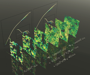
  $\boldsymbol {x}^-$, arbitrarily separated in space (figure 1). Hereafter, the
  $+$ and
  $-$ superscripts denote the quantity at the point
  $\boldsymbol {x}^+$ and
  $\boldsymbol {x}^-$, respectively. Multiplying the equation at
  $\boldsymbol {x}^+$ by
  $\phi ^-$ and the one at
  $\boldsymbol {x}^-$ by
  $\phi ^+$, yields
 \begin{gather} \phi^-\partial_t \phi^+ + \boldsymbol{u}^+ \boldsymbol{\cdot} \phi^-\boldsymbol{\nabla}_{\boldsymbol{x}^+} \phi^+ = \phi^- S_d^+ | \boldsymbol{\nabla}_{\boldsymbol{x}} \phi|^+ , \end{gather}
 \begin{gather}\phi^+ \partial_t \phi^- + \boldsymbol{u}^- \boldsymbol{\cdot} \phi^+\boldsymbol{\nabla}_{\boldsymbol{x}^-} \phi^- = \phi^+ S_d^- | \boldsymbol{\nabla}_{\boldsymbol{x}} \phi|^- . \end{gather}
Since for any quantity  $[\bullet ]$, we have
  $\boldsymbol {\nabla }_{\boldsymbol {x}^+} [\bullet ]^- = \boldsymbol {\nabla }_{\boldsymbol {x}^-} [\bullet ]^+ =0$, one obtains
 \begin{gather} \phi^-\partial_t \phi^+ + \boldsymbol{u}^+ \boldsymbol{\cdot} \boldsymbol{\nabla}_{\boldsymbol{x}^+} \phi^+ \phi^- = \phi^- S_d^+ | \boldsymbol{\nabla}_{\boldsymbol{x}} \phi|^+ , \end{gather}
 \begin{gather}\phi^+ \partial_t \phi^- + \boldsymbol{u}^- \boldsymbol{\cdot} \boldsymbol{\nabla}_{\boldsymbol{x}^-} \phi^+ \phi^- = \phi^+ S_d^- | \boldsymbol{\nabla}_{\boldsymbol{x}} \phi|^- . \end{gather}
Summing up these two equations gives
 \begin{align} & \partial_t \phi^+\phi^- + \boldsymbol{u}^+ \boldsymbol{\cdot} \boldsymbol{\nabla}_{\boldsymbol{x}^+} \phi^+ \phi^- + \boldsymbol{u}^- \boldsymbol{\cdot} \boldsymbol{\nabla}_{\boldsymbol{x}^-} \phi^+ \phi^- \nonumber\\ &\quad = \phi^- S_d^+ | \boldsymbol{\nabla}_{\boldsymbol{x}} \phi|^+ + \phi^+ S_d^- | \boldsymbol{\nabla}_{\boldsymbol{x}} \phi|^-. \end{align}
We now define the mid-point  $\boldsymbol {X} = (\boldsymbol {x}^+ + \boldsymbol{x}^-)/2$ and separation vector
  $\boldsymbol {r} = \boldsymbol {x}^+ - \boldsymbol {x}^-$ (see figure 1). Using the relations
  $\boldsymbol {\nabla }_{\boldsymbol {x}^+} = \frac {1}{2} \boldsymbol {\nabla }_{\boldsymbol {X}} + \boldsymbol {\nabla }_{\boldsymbol {r}}$ and
  $\boldsymbol {\nabla }_{\boldsymbol {x}^-} = \frac {1}{2} \boldsymbol {\nabla }_{\boldsymbol {X}} - \boldsymbol {\nabla }_{\boldsymbol {r}}$ (Hill Reference Hill2002; Danaila et al. Reference Danaila, Antonia and Burattini2004), we obtain
 \begin{align} \partial_t \phi^+\phi^- &= - \boldsymbol{\nabla}_{\boldsymbol{X}} \boldsymbol{\cdot} (\sigma\boldsymbol{u}) \phi^+\phi^- - \boldsymbol{\nabla}_{\boldsymbol{r}} \boldsymbol{\cdot} (\delta \boldsymbol{u}) \phi^+\phi^- \nonumber\\ &\quad + \phi^- S_d^+ | \boldsymbol{\nabla}_{\boldsymbol{x}} \phi|^+ + \phi^+ S_d^- | \boldsymbol{\nabla}_{\boldsymbol{x}} \phi|^- \nonumber\\ &\quad + 2 \phi^+ \phi^- (\sigma \{\boldsymbol{\nabla_x} \boldsymbol{\cdot}\boldsymbol{u}\}). \end{align}
Equation (2.9) is the transport equation for the correlation function of the phase indicator field where  $S_d$ can take any value. Here
  $(\sigma \bullet ) = (\bullet ^+ + \bullet ^-)/2$ and
  $(\delta \bullet ) = (\bullet ^+ - \bullet ^-)$. Note that (2.9) also considers flows in which the velocity divergence may not be zero. This is accounted for in the rightmost term on the right-hand side of (2.9) which reads as the product of
  $\phi ^+ \phi ^-$ and the average of
  $\boldsymbol{\nabla}_{\boldsymbol{x}} \boldsymbol {\cdot }\boldsymbol {u}$ between the two points
  $\boldsymbol {x}^+$ and
  $\boldsymbol {x}^-$.

Figure 1. Schematic representation of two points  $\boldsymbol {x}^+$ and
  $\boldsymbol {x}^-$, the midpoint
  $\boldsymbol {X} = (X,Y,Z)$ and the separation vector
  $\boldsymbol {r} = (r_x, r_y, r_z)$.
The squared increment of  $\phi$, i.e.
  $(\delta \phi ) ^2 = (\phi ^+ - \phi ^-)^2$, is related to
  $\phi ^+ \phi ^-$ by
 \begin{align} \phi^+ \phi^- &= \left(\frac{\phi^+ + \phi^-}{2}\right)^2 - \left(\frac{\phi^+ - \phi^-}{2}\right)^2 \nonumber\\ &= (\sigma \phi)^2 - \frac{(\delta \phi)^2}{4} \nonumber\\ &= \frac{1}{2} \left( \left(\phi^+\right)^2 + \left(\phi^-\right)^2 \right) - \frac{(\delta \phi)^2}{2} \nonumber\\ &= (\sigma \phi) - \frac{1}{2}(\delta \phi)^2. \end{align}
 For obtaining (2.10), use was made of the relation  $\phi ^2 = \phi$ as
  $\phi$ can take only 0 or 1 values. Substituting (2.10) into (2.9), and noting that the transport equation for
  $(\sigma \phi )$ is
 \begin{align} \partial_t (\sigma \phi) &= - \boldsymbol{\nabla}_{\boldsymbol{X}} \boldsymbol{\cdot} (\sigma \boldsymbol{u}) (\sigma \phi) - \boldsymbol{\nabla}_{\boldsymbol{r}} \boldsymbol{\cdot} (\delta \boldsymbol{u}) (\sigma \phi) \nonumber\\ &\quad + \sigma \lbrace S_d |\boldsymbol{\nabla} \phi| \rbrace + 2 (\sigma \phi) (\sigma \{\boldsymbol{\nabla_x}\boldsymbol{\cdot}\boldsymbol{u}\}), \end{align}
we end up with the transport equation for  $(\delta \phi )^2$,
 \begin{align}
\partial_t (\delta \phi)^2 &= - \boldsymbol{\nabla}_{\boldsymbol{X}}
\boldsymbol{\cdot} (\sigma \boldsymbol{u}) (\delta \phi)^2
- \boldsymbol{\nabla}_{\boldsymbol{r}} \boldsymbol{\cdot}
(\delta \boldsymbol{u}) (\delta \phi)^2 \nonumber\\
&\quad + 2 (\sigma \lbrace S_d |\boldsymbol{\nabla} \phi| \rbrace)
- 2 (\phi^- S_d^+ | \boldsymbol{\nabla}_{\boldsymbol{x}}
\phi|^+ + \phi^+ S_d^- | \boldsymbol{\nabla}_{\boldsymbol{x}} \phi|^-) \nonumber\\
&\quad + 2 (\delta \phi)^2 (\sigma
\{\boldsymbol{\nabla}_{\boldsymbol{x}}\boldsymbol{\cdot}\boldsymbol{u}\}).
\end{align}
\begin{align}
\partial_t (\delta \phi)^2 &= - \boldsymbol{\nabla}_{\boldsymbol{X}}
\boldsymbol{\cdot} (\sigma \boldsymbol{u}) (\delta \phi)^2
- \boldsymbol{\nabla}_{\boldsymbol{r}} \boldsymbol{\cdot}
(\delta \boldsymbol{u}) (\delta \phi)^2 \nonumber\\
&\quad + 2 (\sigma \lbrace S_d |\boldsymbol{\nabla} \phi| \rbrace)
- 2 (\phi^- S_d^+ | \boldsymbol{\nabla}_{\boldsymbol{x}}
\phi|^+ + \phi^+ S_d^- | \boldsymbol{\nabla}_{\boldsymbol{x}} \phi|^-) \nonumber\\
&\quad + 2 (\delta \phi)^2 (\sigma
\{\boldsymbol{\nabla}_{\boldsymbol{x}}\boldsymbol{\cdot}\boldsymbol{u}\}).
\end{align} Equation (2.12) is the general expression for the unaveraged squared increments  $(\delta \phi )^2$. It generalizes the equation derived by Thiesset et al. (Reference Thiesset, Duret, Ménard, Dumouchel, Reveillon and Demoulin2020, Reference Thiesset, Ménard and Dumouchel2021) to the case where
  $S_d \neq 0$ and/or
  $\boldsymbol{\nabla}_{\boldsymbol{x}} \boldsymbol {\cdot }\boldsymbol {u} \neq 0$. Compared with the equations detailed by Thiesset et al. (Reference Thiesset, Duret, Ménard, Dumouchel, Reveillon and Demoulin2020, Reference Thiesset, Ménard and Dumouchel2021), where only the unsteady and the two transfer terms (in
  $\boldsymbol {r}$ and
  $\boldsymbol {X}$ space) were present, (2.12) reveals an additional source term which notably depends on the correlation between a quantity related to the bulk phase
  $\phi$ and a surface quantity, namely
  $S_d|\boldsymbol{\nabla}_{\boldsymbol{x}} \phi |$. When estimated numerically, this type of correlation requires a specific treatment which will be described later. The right-hand side of (2.12) also contains an additional nonlinear forcing term which depends on the velocity divergence. In incompressible flows this term vanishes.
As detailed in the following, (2.12) can be applied to very different types of scalar, either passive, active or reacting, in either decaying or forced turbulence, representative of either single or two-phase flows.
(i) In two-phase flows with no phase change,
 $S_d = 0$ and one recovers the equation first derived by Thiesset et al. (Reference Thiesset, Duret, Ménard, Dumouchel, Reveillon and Demoulin2020, Reference Thiesset, Ménard and Dumouchel2021). Material surfaces share also the property $S_d = 0$ (Pope, Yeung & Girimaji Reference Pope, Yeung and Girimaji1989).
(ii) In the case of a passive scalar with no forcing, only
$S_d^d$ contributes to $S_d$. When, for example, a scalar mean gradient $G_\xi$ in a given direction $\alpha$ is superimposed, then another contribution emerges from $S_d^s = u_\alpha G_\xi / |\boldsymbol{\nabla}_{\boldsymbol{x}} \xi |$.(iii) The present framework also applies to premixed flames. Then,
$\xi$ can be associated to the fuel or oxidizer mass fraction or to the temperature field. In this situation, $S_d$ incorporates both $S_d^d$ and $S_d^r$. Diffusion flames can also be analysed using the present framework. In either premixed or diffusion flames, one generally defines $S_d$ in the density weighted manner (Giannakopoulos et al. Reference Giannakopoulos, Frouzakis, Mohan, Tomboulides and Matalon2019). Note also that due to heat release, one should also account for the additional term due to $\boldsymbol{\nabla}_{\boldsymbol{x}} \boldsymbol {\cdot }\boldsymbol {u}$.(iv) In two-phase flows with phase change,
$\xi$ can, for instance, represent the liquid volume fraction and $S_d^r$ relates to the evaporation rate. Here again, one should account for the term due to non-zero velocity divergence. The velocity jump across the interface that originates from the evaporation rate and the density jump between the two phases should also be accounted for.(v) Equation (2.12) also applies to the enstrophy field. In this situation,
$S_d$ contains a contribution due to diffusion effects and an additional forcing term due to vortex stretching (Krug et al. Reference Krug, Holzner, Lüthi, Wolf, Kinzelbach and Tsinober2015). The present framework is thus likely to help in scrutinizing the structure and kinematics of the TNTI which is often defined through a given iso-enstrophy value.


To summarize, the new framework proposed here is very general and enables us to treat a variety of different scalars (passive or reacting scalars, with or without forcing) in different flow situations (single or two-phase flows, in forced or decaying turbulence, in the presence of phase change).
Because the flows under consideration can be turbulent, it is worth supplementing (2.9) and (2.12) by some averaging operators. The choice of a specific average generally depends on the flow situations (Hill Reference Hill2002; Thiesset et al. Reference Thiesset, Duret, Ménard, Dumouchel, Reveillon and Demoulin2020, Reference Thiesset, Ménard and Dumouchel2021). One can simply apply an ensemble average operator, noted  $\langle \bullet \rangle _\mathbb {E}$, which has the advantage of commuting with time
  $t$, spatial
  $\boldsymbol {X}$ and scale
  $\boldsymbol {r}$ derivatives. Hence, the ensemble average of (2.12) is
 \begin{align} \partial_t \langle (\delta \phi)^2 \rangle_\mathbb{E} &= - \boldsymbol{\nabla}_{\boldsymbol{X}} \boldsymbol{\cdot} \langle (\sigma \boldsymbol{u}) (\delta \phi)^2 \rangle_\mathbb{E} - \boldsymbol{\nabla}_{\boldsymbol{r}} \boldsymbol{\cdot} \langle (\delta \boldsymbol{u}) (\delta \phi)^2 \rangle_\mathbb{E} \nonumber\\ &\quad + 2 \langle \sigma \lbrace S_d |\boldsymbol{\nabla} \phi| \rbrace \rangle_\mathbb{E} - 2 (\langle \phi^- S_d^+ | \boldsymbol{\nabla}_{\boldsymbol{x}} \phi|^+ \rangle_\mathbb{E} + \langle \phi^+ S_d^- | \boldsymbol{\nabla}_{\boldsymbol{x}} \phi|^-\rangle_\mathbb{E}) \nonumber\\ &\quad + 2 \langle (\delta \phi)^2 (\sigma \{\boldsymbol{\nabla_x}\boldsymbol{\cdot}\boldsymbol{u}\}) \rangle_{\mathbb{E}}. \end{align}
In the present study we further exploit the statistical symmetry of the flow (see § 3.2) and we will consider a spatial average over a periodic domain of volume  $V_{box}$,
 \begin{equation} \langle \bullet \rangle_\mathbb{R} = \frac{1}{V_{box}} \iiint_{\boldsymbol{X}} \bullet \,{\rm d}\boldsymbol{X}. \end{equation}
Spatial averages commute with time  $t$ and
  $\boldsymbol {r}$ derivatives, but not with the
  $\boldsymbol {X}$ divergence operator. However, by periodicity, the fluxes
  $(\sigma \boldsymbol {u}) (\delta \phi )^2$ normal to the domain boundaries vanish (Hill Reference Hill2002; Thiesset et al. Reference Thiesset, Duret, Ménard, Dumouchel, Reveillon and Demoulin2020). Hence, the transfer term with respect to spatial position
  $\boldsymbol {X}$ is zero. Assuming a divergence-free flow yields
  $\langle (\delta \phi )^2 (\sigma \{\boldsymbol{\nabla}_{\boldsymbol{x}}\boldsymbol {\cdot } \boldsymbol {u}\}) \rangle _{\mathbb {E,R}} = 0$. Statistical homogeneity leads to
  $2 \langle \sigma \lbrace S_d |\boldsymbol {\nabla } \phi |\rbrace \rangle _{\mathbb {E,R}} = \langle S_d |\boldsymbol {\nabla } \phi | \rangle _{\mathbb {E,R}}$ and
  $\langle \phi ^- S_d^+ | \boldsymbol {\nabla }_{\boldsymbol {x}} \phi |^+ \rangle _\mathbb {E} = \langle \phi ^+ S_d^- | \boldsymbol {\nabla }_{\boldsymbol {x}} \phi |^-\rangle _\mathbb {E}$. With these simplifications, (2.12) then writes as
 \begin{equation} \underbrace{\partial_t \langle (\delta \phi)^2 \rangle_\mathbb{E,R}}_{Unsteady} = \underbrace{- \boldsymbol{\nabla}_{\boldsymbol{r}} \boldsymbol{\cdot} \langle (\delta \boldsymbol{u}) (\delta \phi)^2 \rangle_\mathbb{E,R}}_{Transfer\text{-}r}+ \underbrace{2\langle S_d \rangle_s \varSigma - 4 \langle \phi^+ S_d^- |\boldsymbol{\nabla}_{\boldsymbol{x}} \phi|^- | \rangle_\mathbb{E,R}}_{S_d-{Term}},\end{equation}
where  $\varSigma = \langle |\boldsymbol{\nabla}_{\boldsymbol{x}} \phi | \rangle _\mathbb {R}$ is the surface density of the iso-scalar surface, i.e. the area of the iso-scalar surface divided by
  $V_{box}$;
  $\langle \bullet \rangle _s$ denotes the area weighted average. At this stage, (2.15) depends on time
  $t$ and the separation vector
  $\boldsymbol {r}$ (a four-dimensional space). The problem can further be reduced supposing isotropy, i.e. statistical invariance by rotation of the separation vector
  $\boldsymbol {r}$, i.e.
  $\langle \bullet \rangle _\mathbb {R} (\boldsymbol {r}) = \langle \bullet \rangle _\mathbb {R} (|\boldsymbol {r}|)$. In the case of anisotropic flows one can apply an angular average, noted
  $\langle \bullet \rangle _\varOmega$, over all orientations of the vector
  $\boldsymbol {r}$ (Thiesset et al. Reference Thiesset, Ménard and Dumouchel2021),
 \begin{equation} \langle \bullet \rangle_\varOmega = \frac{1}{4{\rm \pi}} \iint_\varOmega \bullet \sin \theta \,{\rm d}\theta \,{\rm d} \varphi, \end{equation}
where the set of solid angles  $\varOmega = \lbrace \varphi, \theta \,|\, 0 \leq \varphi \leq {\rm \pi},\ 0 \leq \theta \leq 2 {\rm \pi}\rbrace$ with
  $\varphi = \arctan (r_y/r_x)$ and
  $\theta = \arccos (r_z/|\boldsymbol {r}|)$ (
 $r_x, r_y, r_z$ denote the components of the
  $\boldsymbol {r}$ vector in
  $x, y, z$ directions, respectively). Spatially and angularly averaged statistics depend on time
  $t$ and scale
  $r$, i.e. the four-dimensional problem was reduced to two dimensions.
2.3. Asymptotic limits at large and small scales
At this stage it is worth recalling that employing two-point statistics of the phase indicator field is not new. It is widely employed for characterizing the microstructure of heterogeneous materials such as porous media, composite material, fractal aggregates and colloids. The reader can refer to Torquato (Reference Torquato2002) where these aspects are discussed in great detail.
Among this wide corpus of literature, it is worth mentioning the work by Kirste & Porod (Reference Kirste and Porod1962) and Frisch & Stillinger (Reference Frisch and Stillinger1963) who proved that, for isotropic-homogeneous media, and by further assuming that the interface separating the two phases is of class  $C^2$, the limit of
  $\langle (\delta \phi )^2\rangle _\mathbb {R}$ at small scales is given by
 \begin{equation} \lim_{r \to 0} \langle (\delta \phi)^2\rangle_\mathbb{R} = \frac{\varSigma r}{2} \left[ 1- \frac{r^2}{8} \left(\langle \mathcal{H}^2\rangle_s - \frac{\langle \mathcal{G}\rangle_s}{3} \right) \right]. \end{equation}
Here,  $\mathcal {H}$ and
  $\mathcal {G}$ are the mean and Gaussian curvatures, respectively;
  $\langle \bullet \rangle _s$ is used to denote the surface area weighted average. Berryman (Reference Berryman1987) and Thiesset et al. (Reference Thiesset, Ménard and Dumouchel2021) proved that (2.17) remains valid in anisotropic media by applying an additional angular average to
  $\langle (\delta \phi ) ^2\rangle _\mathbb {R}$. When
  $|\boldsymbol {r}| \to \infty$, Thiesset et al. (Reference Thiesset, Duret, Ménard, Dumouchel, Reveillon and Demoulin2020, Reference Thiesset, Ménard and Dumouchel2021) showed that
 \begin{equation} \lim_{r \to \infty} \langle (\delta \phi) ^2\rangle_\mathbb{R} = 2\langle \phi \rangle_\mathbb{R} (1-\langle \phi \rangle_\mathbb{R}). \end{equation}
The limit of  $\langle \phi ^+ |\boldsymbol{\nabla}_{\boldsymbol{x}} \phi |^- \rangle _\mathbb {R}$ as
  $|\boldsymbol {r}|$ tends to zero can be expressed as (Teubner Reference Teubner1990)
 \begin{equation} \lim_{r \to 0} \langle \phi^+ |\boldsymbol{\nabla_x} \phi |^- \rangle_\mathbb{R} = \frac{\varSigma }{2} \left[ 1 + \frac{r}{2} \langle \mathcal{H}\rangle_s \right]. \end{equation}
As far as we are aware, the next terms of the small-scale expansion of  $\langle \phi ^+ |\boldsymbol{\nabla}_{\boldsymbol{x}} \phi |^- \rangle _\mathbb {R}$ are not known. In the limit of large separations, we have (Teubner Reference Teubner1990)
 \begin{equation} \lim_{r \to \infty} \langle \phi^+ |\boldsymbol{\nabla_x} \phi |^- \rangle_\mathbb{R} = \langle \phi \rangle_{\mathbb{R}}\varSigma . \end{equation}
The special case  $\langle \phi \rangle _{\mathbb {R}} = 0.5$ yields
  $\langle \phi ^+ |\boldsymbol{\nabla}_{\boldsymbol{x}} \phi |^- \rangle _\mathbb {R} (r) = \varSigma / 2$. Equation (2.19) suggests that, when
  $|\boldsymbol {r}| \to 0$,
  $\langle \phi ^+ S_d^- |\boldsymbol{\nabla}_{\boldsymbol{x}} \phi |^- \rangle _\mathbb {R}$ writes as
 \begin{equation} \lim_{r \to 0} \langle \phi^+ S_d^-|\boldsymbol{\nabla_x} \phi |^- \rangle_\mathbb{R} = \frac{\varSigma }{2} \left[ \langle S_d \rangle_s + \frac{r}{2} \langle \mathcal{H}S_d\rangle_s \right] , \end{equation}
while at large scales one may write
 \begin{equation} \lim_{r \to \infty} \langle \phi^+ S_d^-|\boldsymbol{\nabla_x} \phi |^- \rangle_\mathbb{R} = \langle \phi \rangle_{\mathbb{R}} \langle S_d\rangle_s \varSigma. \end{equation}
As discussed by Thiesset et al. (Reference Thiesset, Ménard and Dumouchel2021), (2.17) and similarly (2.19) and (2.21) apply up to a separation  $r$, which is twice the ‘reach’ of the surface. The ‘reach’ is a notion that pertains to non-convex bodies. It is defined as the minimal normal distance between the surface and its medial axis (see, e.g. Federer Reference Federer1959). The medial axis of a given body is the set of all points having more than one closest point on the object's boundary. It can also be seen as the location of centres of all bi-tangent spheres, i.e. the spheres that are tangent to the surface in at least two points on the surface. The reach is thus given by the minimal radius of these bi-tangent spheres. In some special situations (in the absence of narrow throats or necks) it can be related to the minimal radius of curvature. Otherwise, it relates to the smallest narrow throat or neck. For scales larger than the reach,
  $\langle (\delta \phi )^2 \rangle _\mathbb {R}$ contains information about the morphology of the structures under hand. In this respect, Adler et al. (Reference Adler, Jacquin and Quiblier1990), Torquato (Reference Torquato2002) and Thiesset et al. (Reference Thiesset, Ménard and Dumouchel2021) showed that the scale distribution
  $\langle \phi ^+ \phi ^- \rangle _\mathbb {R}$ or
  $\langle (\delta \phi )^2 \rangle _\mathbb {R}$ widens when the morphological content (or its tortuousness) of a given set increases. Similarly, the fractal facets of aggregates are often appraised by use of the correlation function of the phase indicator at intermediate scales (see, e.g. Sorensen Reference Sorensen2001). In particular, Morán et al. (Reference Morán, Fuentes, Liu and Yon2019) showed that when increasing the ratio between the largest scales (the aggregate radius of gyration) and the smallest scales (the radius of the primary particle), the correlation function reveals an increasing range of scales complying with a fractal scaling (a power law). Vassilicos & Hunt (Reference Vassilicos and Hunt1991), Vassilicos (Reference Vassilicos1992) and Vassilicos & Hunt (Reference Vassilicos and Hunt1996) showed that
  $\langle (\delta \phi )^2\rangle _\mathbb {E}$ might reveal a power-law behaviour whose exponent is related to the fractal dimension (more precisely the Kolmogorov capacity) of iso-scalar surfaces. This was investigated in great detail by Elsas et al. (Reference Elsas, Szalay and Meneveau2018) for the enstrophy, dissipation and velocity gradient invariants. When several structures are present,
  $\langle (\delta \phi )^2\rangle _\mathbb {E,R}$ also depends on the way the different fluid structures are organized in space. The reach of the surface plays an important role here since it is the scale which separates the zones in scale space where
  $\langle (\delta \phi )^2 \rangle _\mathbb {R}$ depends only on integral geometric measures (
 $\varSigma$,
  $\langle \mathcal {H}^2\rangle _s$,
  $\langle \mathcal {G}\rangle _s$) and the range of scales for which two-point statistics become a morphological descriptor (Torquato Reference Torquato2002) for which both the geometry and the additional information about the medial axis is required for the structure to be characterized. For scales larger than the reach, the separation
  $r$ cannot be interpreted as the size of the structure under consideration (as it will be seen later, the correlation
  $\langle \phi ^+\phi ^- \rangle _\mathbb {R}$ tends to 0 when the scale
  $r$ is similar to the size of the structure), but should rather be referred to as the morphological parameter as it is generally done in morphological analysis using, for example, integral geometrical measures (the Minkowski functional) of parallel sets (Arns, Knackstedt & Mecke Reference Arns, Knackstedt and Mecke2004; Dumouchel, Thiesset & Ménard Reference Dumouchel, Thiesset and Ménard2022).
Given the asymptotic limits detailed in the previous section, it seems natural to examine the limit at small and large scales of (2.12) (or (2.9)). In Thiesset et al. (Reference Thiesset, Ménard and Dumouchel2021) it was demonstrated that (2.12) naturally converges to the transport equation for the surface density when  $|\boldsymbol {r}| \to 0$. The latter can be written in the form (Pope Reference Pope1988; Candel & Poinsot Reference Candel and Poinsot1990; Drew Reference Drew1990; Blakeley, Wang & Riley Reference Blakeley, Wang and Riley2019)
 \begin{equation} \partial_t \varSigma + \boldsymbol{\nabla}_{\boldsymbol{x}} \boldsymbol{\cdot} \langle \boldsymbol{u} \rangle_s \varSigma = (\mathbb{K}_T + \mathbb{K}_C) \varSigma, \end{equation}
where the stretch rate  $\mathbb {K} = \mathbb {K}_T + \mathbb {K}_C$ measures the relative time increase of surface density;
  $\mathbb {K}_T$ denotes the tangential strain rate that may include compressibility effect, and
  $\mathbb {K}_C = - 2 \langle S_d \mathcal {H} \rangle _s$ is the curvature component of the stretch rate.
Thiesset et al. (Reference Thiesset, Ménard and Dumouchel2021) considered the case where  $S_d = 0$ (a material surface as in two-phase flows) and showed that, in the limit of small separations, the
  $\boldsymbol {X}$-transport term in (2.12) asymptotes the convection process of the surface density
  $\varSigma$ (the rightmost term on the left-hand side (2.23)) while the unsteady term in (2.12) obviously tends to the unsteady term in (2.23). Thiesset et al. (Reference Thiesset, Ménard and Dumouchel2021) argued that by difference, the
  $\boldsymbol {r}$-transfer term is proportional to the strain rate
  $\mathbb {K}_T$, viz.
 \begin{equation} \lim_{r\to 0} \left[ -\boldsymbol{\nabla_r} \boldsymbol{\cdot} \langle (\delta \boldsymbol{u}) (\delta \phi)^2\rangle_\mathbb{R} \right]= \mathbb{K}_T \varSigma \frac{r}{2}. \end{equation}
Note that here again, this holds true in anisotropic configuration by using an additional angular average. When the interface displacement speed is not zero, the right-hand side of (2.12) has the following asymptotic limit:
 \begin{align} & \lim_{r \to 0} \left[ 2
\left(\sigma \langle S_d |\boldsymbol{\nabla} \phi|
\rangle_\mathbb{R}\right) - 2 \left( \langle \phi^- S_d^+ |
\boldsymbol{\nabla}_{\boldsymbol{x}} \phi|^+
\rangle_\mathbb{R} + \langle \phi^+ S_d^- |
\boldsymbol{\nabla}_{\boldsymbol{x}}
\phi|^-\rangle_\mathbb{R} \right) \right]\nonumber\\
&\quad = 2 \langle S_d \rangle_s \varSigma - 2 \varSigma
\left(\langle S_d \rangle_s + \langle S_d
\mathcal{H}\rangle_s \frac{r}{2}\right) \nonumber\\ &\quad
= - 2 \langle S_d \mathcal{H}\rangle_s \varSigma
\frac{r}{2} \nonumber\\ &\quad = \mathbb{K}_C \varSigma
\frac{r}{2}. \end{align}
\begin{align} & \lim_{r \to 0} \left[ 2
\left(\sigma \langle S_d |\boldsymbol{\nabla} \phi|
\rangle_\mathbb{R}\right) - 2 \left( \langle \phi^- S_d^+ |
\boldsymbol{\nabla}_{\boldsymbol{x}} \phi|^+
\rangle_\mathbb{R} + \langle \phi^+ S_d^- |
\boldsymbol{\nabla}_{\boldsymbol{x}}
\phi|^-\rangle_\mathbb{R} \right) \right]\nonumber\\
&\quad = 2 \langle S_d \rangle_s \varSigma - 2 \varSigma
\left(\langle S_d \rangle_s + \langle S_d
\mathcal{H}\rangle_s \frac{r}{2}\right) \nonumber\\ &\quad
= - 2 \langle S_d \mathcal{H}\rangle_s \varSigma
\frac{r}{2} \nonumber\\ &\quad = \mathbb{K}_C \varSigma
\frac{r}{2}. \end{align}
Consequently, the additional term in the two-point budget due to the presence of an interface displacement speed asymptotes, in the limit of small separations, to the curvature component of the stretch rate.
Similarly, given that at large scales the  $r$-transfer term tends to zero, (2.12) should provide insights into the excursion set volume equation. We indeed obtain that at large scales the budget simplifies to
 \begin{align} \lim_{r \to \infty} \partial_t \langle (\delta \phi)^2\rangle_{\mathbb{R}} &= 2 (1-2\langle \phi\rangle_\mathbb{R}) \partial_t \langle \phi\rangle_\mathbb{R} \nonumber\\ &= 2 (1-2\langle \phi\rangle_\mathbb{R}) \langle S_d \rangle_s \varSigma, \end{align}
where use was made of the equation for the volume (Drew Reference Drew1990)
 \begin{equation} \partial_t \langle \phi\rangle_\mathbb{R} = \langle S_d \rangle_s \varSigma. \end{equation}
 Note that the volume of the excursion set  $\langle \phi \rangle _\mathbb {R}$ reads as the probability that
  $\xi (\boldsymbol {x})>\xi _0$. It is thus related to the cumulative distribution of
  $\xi (\boldsymbol {x})$. Assuming a Gaussian distribution for the scalar field
  $\xi (\boldsymbol {x},t)$,
  $\langle \phi \rangle _\mathbb {R}$ can be written analytically as
 \begin{equation} \langle \phi \rangle_\mathbb{R} = \frac{1}{2} \left( 1 - {\rm erf}\left(\frac{\xi_0}{\sqrt{2} \xi_{rms}} \right)\right), \end{equation}
where the subscript ‘rms’ stands for the standard deviation of the considered quantity. To dig a little deeper in the interpretation of  $\langle (\delta \phi )^2 \rangle _\mathbb {R}$, we can resort to some tools from mathematical morphology. This analysis is carried out in Appendix A, where we provide a handy demonstration that at intermediate scales,
  $\langle (\delta \phi )^2 \rangle _\mathbb {R}$ measures the morphological content of the sets under consideration. The structure function is thus here aptly named since it is a function that depends on the structure (actually the microstructure) of the fluid elements. It allows some geometrical features of iso-scalar sets to be inferred such as its volume, the surface area, mean and Gaussian curvatures, and its transport equation naturally approaches the transport equations of surface density and volume at respectively small and large scales. Note that by virtue of the Gauss–Bonnet theorem, the presence of
  $\langle \mathcal {G} \rangle _s$ in (2.17) indicates that
  $\langle (\delta \phi )^2 \rangle _\mathbb {R}$ depends also on the topology (the Euler characteristic) of the field under consideration.
Consequently, the present set of equations allows not only the morphology of scalar excursion sets to be described, it also accounts for its kinematic evolution through (2.9) or (2.12). The interface retains through its geometry and kinematics the signature of the flow dynamics and, in some instances (e.g. two-phase flows, TNTI), may even influence the whole flow dynamics. Therefore, we like referring to this framework as a morphodynamical theory since it is likely to provide insights into the morphological evolution of fluid elements.
3. Numerical database and post-processing
3.1. Direct numerical simulation of scalar mixing in decaying turbulence
The present analytical framework is appraised using data from DNS. We studied two flow configurations, i.e. forced turbulence (denoted by the ‘F’ letter in table 1) and decaying turbulence (denoted by the letter ‘D’ in table 1). We have also one case, noted ‘T’, which was used for tests and validation purposes. Table 1 gathers all important simulation parameters and related statistical quantities, where  $N$ denotes the number of grid points along one coordinate axis,
  $\nu$ is the kinematic viscosity, and
 \begin{equation} R_\lambda=\frac{u_{rms}\lambda}{\nu} \end{equation}
is the Reynolds number based on the Taylor microscale  $\lambda =\sqrt {15 \nu u_{rms}^2 / \langle \epsilon \rangle }$, where
  $u_{rms}$ is the root-mean-square velocity,
  $\langle k\rangle = \langle u_i u_i \rangle /2$ is the mean kinetic energy and
  $\langle \epsilon \rangle = 2 \nu \langle \mathcal {S}_{ij} \mathcal {S}_{ij} \rangle$ is the mean energy dissipation rate, with the strain rate tensor given by
  $\mathcal {S}_{ij} = (\partial u_i / \partial x_j + \partial u_j /\partial x_i)/2$. Furthermore,
  $\langle \xi ^2 \rangle$ denotes the mean scalar variance,
  $\langle \epsilon _\xi \rangle = 2D \langle (\partial \xi / \partial x_i)^2 \rangle$ is the mean scalar dissipation rate and
  $\lambda _\xi = \sqrt {6 D \langle \xi ^2 \rangle / \langle \epsilon _\xi \rangle }$ denotes the Corrsin length scale;
  $L_t$ and
  $L_\xi$ denote the integral length scales of the velocity and scalar fields, respectively. The Kolmogorov and the Batchelor length scales are defined as
 \begin{equation} \eta = \left( \frac{\nu^3}{\langle \epsilon \rangle} \right)^{1/4} \quad \text{and} \quad \eta_B= \left( \frac{\nu D^2}{\langle \epsilon \rangle} \right)^{1/4} = \frac{\eta}{Sc^{1/2}}, \end{equation}
respectively. The turbulent Péclet number  $\mathit {Pe}_{\lambda _\xi }$ is defined in § 4.5.
Table 1. Physical parameters and typical one-point statistics of the DNS database used in the present work.

(i) The forced turbulence database encompasses six different values of Taylor-based Reynolds numbers
$R_\lambda$ (cases F0 to F5 in table 1) from 88 to 530. For the lowest Reynolds number (F0, $R_\lambda = 88$), we carried out another simulation with four different scalar fields with different diffusion coefficients $D$, which correspond to Schmidt number variations from $Sc = 0.1$ to $1.0$. The numerical database for case F0 ($Sc=1.0$) to F5 is the same as the one used in Gauding et al. (Reference Gauding, Goebbert, Hasse and Peters2015) and Gauding, Danaila & Varea (Reference Gauding, Danaila and Varea2017). To maintain a statistically steady state, an external stochastic forcing is applied to the velocity field (Eswaran & Pope Reference Eswaran and Pope1988). The forcing is statistically isotropic and limited to low wavenumbers to avoid the small scales being affected by the forcing scheme. The passive scalar field is fed by a uniform mean scalar gradient $G_\xi$ which is applied in the $y$-direction. Hence, the scalar field $\tilde \xi$ can be decomposed into a mean field $G_\xi y$ and a fluctuating field $\xi$, i.e.
(3.3)The value of the mean scalar gradient\begin{equation} \tilde \xi = G_\xi y + \xi. \end{equation}$G_\xi$ is set to unity without loss of generality. The indicator function is defined on the fluctuating field $\xi$, which is statistically homogeneous but not isotropic. The statistical anisotropy that is induced by the mean scalar gradient is further discussed in Appendix F. A resolution condition of $\kappa _{max} \eta >2.5$ (where $\kappa _{max}$ is the maximum wavenumber achievable on the numerical grid and $\eta$ the Kolmogorov length scale) is maintained for all cases. As a consequence, the number of grid points has been increased to as high as $N=4096^3$ for case F5. The statistics presented in table 1 and throughout the paper correspond to spatial and ensemble averages over $M$ statistically independent snapshots. Here $M$ varies between 6 for case F5 to 106 for case F0. We have checked that the number of independent snapshots $M$ was sufficient for two-point statistics to be converged. Some tests are reported in Appendix G(ii) For the decaying turbulence case, we explored two distinct situations, the first where the uniform imposed mean scalar gradient is maintained (case D0) and another where both the velocity and scalar field are decaying (case D1). For both D0 and D1, we have carried out DNS for two values of the Schmidt number (0.2 and 1.0). The initial velocity field is generated in spectral space to be random and statistically isotropic. It satisfies incompressibility and obeys a prescribed energy spectrum, i.e.
(3.4)where\begin{equation} E(\kappa,t=0) \propto \kappa^4 \exp \left( -2 \left( \frac{\kappa}{\kappa_p} \right)^2\right), \end{equation}$\kappa _p$ is the wavenumber at which the initial energy spectrum has its peak. We chose $\kappa _p=15$ as a compromise between limiting confinement effects and the goal of reaching a high Reynolds number. The initial mean kinetic energy $\langle k \rangle$ equals 10 leading to an initial Reynolds number, defined as $u_{rms}(t=0)/(\nu \kappa _p)$, as large as 689. For case D0, the scalar field is initialized to zero, allowing scalar structures to develop naturally from the injection of energy through the imposed mean scalar gradient. For case D1, the scalar field decays freely from a prescribed spectrum, which is identical to the energy spectrum of the velocity field given by (3.4) with the same initial peak wavenumber $\kappa _p$. Values reported in table 1 and throughout the paper were obtained at time $t=10$, which is about one decade after the onset of the exponential decay of the kinetic energy. At this time, turbulence is highly resolved with a resolution condition $\kappa _{max}\eta =12.5$. For more details on the set-up of the simulations, see Gauding et al. (Reference Gauding, Wang, Goebbert, Bode, Danaila and Varea2019).(iii) The test case T0 corresponds to decaying turbulence, but with a mesh size of
$512^3$. This allowed us to test the appropriateness of the post-processing procedures. These validations are presented in the Appendices B and C and discussed hereafter in the paper.


The present DNS data were obtained by solving the Navier–Stokes equations and a scalar advection–diffusion equation using a dealiased pseudo-spectral approach. For dealiasing, a filter procedure proposed by Hou & Li (Reference Hou and Li2007) is used, which ensures stability and inhibits spurious oscillations in real space. For cases F0–F5, a second-order semi-implicit Adams–Bashforth/Crank–Nicolson method is used for temporal integration. For the decaying turbulence simulations D0–D1, a low-storage, stability preserving, third-order Runge–Kutta scheme is employed, where for stability, the viscous and diffusive terms are treated by an integrating factor technique. For all cases, the numerical domain is a triply periodic box with length  $L_{box} = 2{\rm \pi}$. The simulations have been carried out with an in-house hybrid MPI/OpenMP parallelized simulation code on the supercomputer JUQUEEN at research center Jülich, Germany.
We show some typical snapshots of the  $\xi (\boldsymbol {x})=0$ iso-surface for different values of the Schmidt and Reynolds numbers in figure 2. We show only a
  $2{\rm \pi} \times 2{\rm \pi} \times {\rm \pi}/2$ subset of the simulated domain. The interface is coloured by the displacement speed
  $S_d$ which is normalized by the velocity standard deviation
  $u_{rms} = 2 \langle k \rangle / 3$. The colour scale covers the range
  $-1 \leq S_d / u_{rms} \leq 1$. Note that although figure 2 gives another impression (remember that only a subset of the domain is presented here), the volume fraction formed by the iso-scalar
  $\xi (\boldsymbol {x})=0$ is the same for all cases and is equal to 0.5. We note that while keeping
  $R_\lambda$ constant (the three leftmost figures in figure 2), a Schmidt number variation from 1 to 0.1 yields a substantial decrease of surface density. The interface is less wrinkled and the corrugation covers a narrower range of scales. This highlights the role of diffusion on the iso-surface geometrical quantities. On the other hand, an increase of the Reynolds number (the four rightmost figures in figure 2) is followed by the creation of smaller and smaller wrinkles and an increase of the morphological content of the iso-scalar volume. Thus,
  $\langle (\delta \phi )^2\rangle _\mathbb {R,E}$ is believed to widen with
  $R_\lambda$. Figure 2 also reveals that the displacement speed
  $S_d$ varies mostly in zones of high curvature. This suggests that the curvature of the interface might play a crucial role for understanding the variations of the displacement speed and its different components.

Figure 2. Iso-surface coloured by the displacement speed  $S_d$ for increasing Schmidt numbers or Reynolds numbers: (a) F0,
  $Sc=0.1$, (b) F0,
  $0.4$, (c) F0,
  $1.0$, (d) F2, (e) F4, ( f) F5.
3.2. Post-processing procedure
The computation of two-point statistics is challenging as it involves the execution of a convolution operation. We compute two-point statistics accurately in real space by a hybrid MPI/OpenMP parallelization employing the two-dimensional pencil domain decomposition of the DNS code. The partial angular average is approximated by averaging over the  $r_x$-,
  $r_y$- and
  $r_z$-directions. Special attention is required for the transfer term, which involves the divergence of a two-point quantity. To avoid the assumption of isotropy, the transfer term is approximated by a second-order finite difference scheme. For instance, in the
  $r_x$-direction, the transfer term reads as
 \begin{align} & \boldsymbol{\nabla}_{\boldsymbol{r}} \boldsymbol{\cdot} \langle (\delta \boldsymbol{u}) (\delta \phi)^2 \rangle_\mathbb{R} (r_x,0,0) \nonumber\\ &\quad \approx\frac{1}{2 {\rm \Delta} r_x} \left[\langle (\delta {u_x}) (\delta \phi)^2 \rangle_\mathbb{R}(r_x+{\rm \Delta} r_x,0,0) - \langle (\delta {u_1}) (\delta \phi)^2 \rangle_\mathbb{R}(r_x-{\rm \Delta} r_x,0,0)\right] \nonumber\\ &\qquad + \frac{1}{2 {\rm \Delta} r_y} \left[ \langle (\delta {u_y}) (\delta \phi)^2 \rangle_\mathbb{R}(r_x,{\rm \Delta} r_y,0) - \langle (\delta {u_2}) (\delta \phi)^2 \rangle_\mathbb{R}(r_x,-{\rm \Delta} r_y,0)\right] \nonumber\\ &\qquad +\frac{1}{2 {\rm \Delta} r_z} \left[ \langle (\delta {u_z}) (\delta \phi)^2 \rangle_\mathbb{R}(r_x,0,{\rm \Delta} r_z) - \langle (\delta {u_3}) (\delta \phi)^2 \rangle_\mathbb{R}(r_x,0,-{\rm \Delta} r_z)\right], \end{align}
where  ${\rm \Delta} r_i$ is the grid spacing and
  $u_x$,
  $u_y$ and
  $u_z$ are the velocity component in the
  $x$,
$x$,  $y$ and
  $z$ directions, respectively. The transfer terms in the
  $r_y$- and
  $r_z$-directions are obtained by a similar procedure.
Some two-point statistics were also computed over the whole  $\boldsymbol {r}$ space using the routines available through the increments library of the project pyarcher (Thiesset & Poux Reference Thiesset and Poux2020). Because six nested loops are needed to cover the whole
  $(\boldsymbol {X},\boldsymbol {r})$-space, we make use of an openMP parallelization for enhancing the calculation speed. Full three-dimensional (3-D) two-point distributions were estimated only for cases F0 and T0 and limited to the range of scales
  $-96\,{{\rm d}x} \leq (r_x, r_y, r_z) \leq 96dx$ where most of the processes take place. By doing so, we are able to check that the partial angular average that operated only over the
  $r_x$-,
  $r_y$- and
  $r_z$-directions lead to results similar to those obtained from the full angular average over the whole set of solid angles. These tests are presented in Appendix C and show that the partial angular average yields similar results to the full angular average. In what follows, only the results for the partial angular average will be presented.
Compared with the equation derived by Thiesset et al. (Reference Thiesset, Duret, Ménard, Dumouchel, Reveillon and Demoulin2020), the influence of the interface displacement results in an additional source term in (2.12). The latter highlights a correlation of the bulk phase  $\phi$ with the surface quantity
  $S_d|\boldsymbol{\nabla}_{\boldsymbol{x}} \phi |$. Hence, this term requires a special treatment. Here, we adapt and develop a procedure inspired by the method of Seaton & Glandt (Reference Seaton and Glandt1986). The reader is advised to refer to Appendix B for a description and a validation of the method.
The geometrical properties of the iso-surface (local surface area, mean and Gaussian curvatures, surface conditional statistics) are extracted using the surface_operators routines of pyarcher. These are earlier versions of the routines described by Essadki et al. (Reference Essadki, Drui, Larat, Ménard and Massot2019) and Di Battista et al. (Reference Di Battista, Bermejo-Moreno, Ménard, de Chaisemartin and Massot2019), now available through the project Mercur(v)e.
4. Results
4.1. Surface conditional statistics
The analytical section presented above reveals that the displacement speed  $S_d$ contains many of the key physics in the behaviour of iso-scalar surfaces. Depending on the situation, it may incorporate different processes such as diffusion, chemical reactions or any other source terms acting on the scalar field. It is thus important to understand how
  $S_d$ evolves along the iso-surface when
  $R_\lambda$ and/or
  $Sc$ are varied. In our situation, the displacement speed contains up to three components, one due to diffusion in the normal direction noted
  $S_d^n$, another due to diffusion in the tangential direction
  $S_d^c = 2D\mathcal {H}$ and a last contribution associated with the imposed mean scalar gradient noted
  $S_d^s$. Their respective expressions are summarized in table 2.
Table 2. Expression of the different components of the displacement speed in forced turbulence with a mean scalar gradient  $G_\xi$.

As it is generally done in reacting flows (Gran et al. Reference Gran, Echekki and Chen1996; Peters et al. Reference Peters, Terhoeven, Chen and Echekki1998), the variations of  $S_d$ along the surface
  $\xi (\boldsymbol {x},t)=\xi _0$ are analysed through the surface weighted average of its different components conditioned on the mean curvature
  $\mathcal {H}$. These surface conditioned statistics are noted
  $\langle S_d^i|\mathcal {H}\rangle _s$ (
 $i = \lbrace c, n, s\rbrace$ denotes the contribution to the displacement speed). Such conditional statistics are relevant notably for providing insights into the curvature component of the stretch rate
  $\mathbb {K}_C$, which reads as the mean product of the displacement speed
  $S_d$ by the mean curvature
  $\mathcal {H}$.
We first analyse the effect of  $R_\lambda$ on
  $S_d$ and its components. Surface conditioned statistics of
  $S_d$,
  $S_d^d$ and
  $S_d^c$ are portrayed in figure 3(a), while those of
  $S_d^n$ and
  $S_d^s$ are displayed in figure 3(b). We consider here an iso-value of
  $\xi _0=0$. Note that in figure 3(a) the ordinate axis is ten times larger than the one in figure 3(b), which shows that the source term and normal diffusion contributions of
  $S_d$ are much smaller than the tangential diffusion component. Therefore, assuming
  $S_d \approx 2D\mathcal {H}$ appears as a reasonable assumption irrespective of the Reynolds number. In figure 3(b) we also note that variations of
  $S_d^s$ decrease in amplitude when
  $R_\lambda$ increases. This suggests that the contribution due to the mean scalar gradient might become negligible at sufficiently large
  $R_\lambda$. It is worth noting that the normal diffusion component of the displacement speed
  $S_d^n$ reveals a non-monotonic evolution with respect to the mean curvature
  $\mathcal {H}$. When the surface is only slightly curved (
 $|\mathcal {H}|$ is small),
  $S_d^n$ is negative (positive) for positive (negative) values of
  $\mathcal {H}$, while the contrary is observed for highly curved regions. The variations of
  $S_d^n$ with the mean curvature does not depend on the Reynolds number for small values of
  $\mathcal {H}$.

Figure 3. Surface averaged displacement speed and its components conditioned on the mean curvature  $\mathcal {H}$ for
  $\xi _0=0$. From dark to light, case F0 (
 $Sc=1.0$) to F4. In (a)
  $S_d$ (full lines),
  $S_d^d$ (dashed lines) and
  $S_d^c$ (dotted lines) are portrayed while
  $S_d^n$ (dashed lines) and
  $S_d^s$ (full lines) are displayed in (b).
The results for different Schmidt numbers are displayed in figure 4. One notes again that the tangential diffusion component of the displacement speed  $S_d^c$ is predominant, thereby emphasizing the role played by curvature. All curves collapse relatively well when the mean curvature is scaled by the scalar diffusivity
  $D$. When the Schmidt number decreases, the contribution due to the source term
  $S_d^s$ increases and so does the normal diffusion contribution
  $S_d^n$.

Figure 4. Surface averaged displacement speed and its components conditioned by the mean curvature  $\mathcal {H}$ for
  $\xi _0=0$. From dark to light, case F0,
  $Sc=1.0$ to
  $Sc=0.1$. In (a)
  $S_d$ (full lines),
  $S_d^d$ (dashed lines) and
  $S_d^c$ (dotted lines) are portrayed while
  $S_d^n$ (dashed lines) and
  $S_d^s$ (full lines) are displayed in (b).
The different components of the displacement speed  $\langle S_d^i \,|\, \mathcal {H} \rangle _s$ for a different iso-scalar value
  $\xi _0 = \xi _{rms}$ are plotted in figures 5 and 6, respectively. We note here again that
  $S_d^s$ and
  $S_d^n$ are about 3 to 10 times smaller in amplitude than
  $S_d^d$ and
  $S_d^c$. In contrast with
  $\xi _0 = 0$,
  $S_d^n$ appears positive for all values of curvature and irrespective of the Schmidt and Reynolds numbers. Although the trends are quantitatively different from what was observed for
  ${\xi _0 = 0}$, we note that
  $S_d$ remains strongly dependent to
  $\mathcal {H}$. In addition, a careful examination of figure 5 reveals that when
  $R_\lambda$ increases, the contribution of
  $S_d^s$ and
  $S_d^n$ decreases which leads to a better correlation between
  $S_d$ and
  $2D\mathcal {H}$. We can speculate that at asymptotically large
  $R_\lambda$, the assumption
  $S_d \approx 2D\mathcal {H}$ holds true irrespective of the iso-scalar value. At constant
  $R_\lambda$, the contribution of
  $S_d^s$ and
  $S_d^n$ increases when the scalar diffusivity increases (figure 6). This suggests that the different contributions to
  $S_d$ for a different iso-level
  $\xi _0$ should be better studied in terms of the Péclet number. In this context, we expect
  $S_d \approx 2D \mathcal {H}$ to hold with better accuracy when the Péclet number increases.

Figure 5. Surface averaged displacement speed and its components conditioned on the mean curvature  $\mathcal {H}$ for
  $\xi _0=\xi _{rms}$. From dark to light, case F0 (
 $Sc=1.0$) to F4. In (a)
  $S_d$ (full lines),
  $S_d^d$ (dashed lines) and
  $S_d^c$ (dotted lines) are portrayed while
  $S_d^n$ (dashed lines) and
  $S_d^s$ (full lines) are displayed in (b).

Figure 6. Surface averaged displacement speed and its components conditioned by the mean curvature  $\mathcal {H}$ for
  $\xi _0=\xi _{rms}$. From dark to light, case F0,
  $Sc=1.0$ to
  $Sc=0.1$. In (a)
  $S_d$ (full lines),
  $S_d^d$ (dashed lines) and
  $S_d^c$ (dotted lines) are portrayed while
  $S_d^n$ (dashed lines) and
  $S_d^s$ (full lines) are displayed in (b).
It is worth finally stressing that our conclusion that the tangential diffusion dominates over the other components of the displacement speed, is built upon the observations of surface weighted averaged values conditioned by the mean curvature  $\mathcal {H}$. This observable cannot reveal how
  $S_d$ and its components are statistically distributed for a given
  $\mathcal {H}$. There is nothing precluding that locally, for a given value of mean curvature, the normal diffusion and/or the source term contributions to
  $S_d$ dominate over the tangential diffusion. This is likely to be observed for low amplitudes of
  $\mathcal {H}$ where the probability density function of
  $\mathcal {H}$ is generally concentrated. More insights into this aspect could be provided by studying the joint probability density function of
  $S_d^i$ and
  $\mathcal {H}$. This is far beyond the scope of the present work and is left for future investigations.
4.2. Second-order structure functions
The present framework is first invoked to explore the dynamics of iso-scalars with an imposed mean scalar gradient in stochastically forced turbulence. In this situation both the flow and scalar characteristics are statistically stationary and the displacement speed has two components, one arising from the diffusive term  $S_d^d$, and one due to the imposed mean gradient
  $S_d^s$. We focus on the particular effect of the Reynolds and Schmidt numbers.
The Reynolds number dependence of  $\langle (\delta \phi )^2\rangle _{\mathbb {R}, \mathbb {E}, \varOmega }$ for different values of the iso-scalar is first considered. Results are presented in figure 7 for
  $R_\lambda$ ranging from 88 to 530 and for two values of the iso-scalar, i.e.
  $\xi _0 = 0$ (figure 7a) and
  $\xi _0 = \xi _{rms}$ (figure 7b). Here
  $\langle (\delta \phi )^2\rangle _{\mathbb {R}, \mathbb {E}, \varOmega }$ is normalized by its asymptotic value at large scales, i.e.
  $2 \langle \phi \rangle _{\mathbb {E}, \mathbb {R}} (1 - \langle \phi \rangle _{\mathbb {E}, \mathbb {R}})$ while the separation
  $r$ is normalized by
  $L_\varSigma = 4\langle \phi \rangle _{\mathbb {E}, \mathbb {R}} (1 - \langle \phi \rangle _{\mathbb {E}, \mathbb {R}})/\varSigma$. Using the normalization with
  $L_\varSigma = 4\langle \phi \rangle _{\mathbb {E}, \mathbb {R}} (1 - \langle \phi \rangle _{\mathbb {E}, \mathbb {R}})/\varSigma$, the asymptotic limits at large and small scales intersect at
  $r/L_\varSigma = 1$. Our definition for
  $L_\varSigma$ finds its inspiration in Lebas et al. (Reference Lebas, Menard, Beau, Berlemont and Demoulin2009) and Thiesset et al. (Reference Thiesset, Duret, Ménard, Dumouchel, Reveillon and Demoulin2020). A somehow similar definition for
  $L_\varSigma$ was conjectured by Peters (Reference Peters1992) for premixed flames. In the context of the Bray–Moss–Libby model (Bray & Moss Reference Bray and Moss1977; Libby & Bray Reference Libby and Bray1980),
  $L_\varSigma$ is known as the wrinkling scale (Kulkarni et al. Reference Kulkarni, Buttay, Kasbaoui, Attili and Bisetti2021), although the surface density is defined differently by the latter authors.

Figure 7. Evolution of  $\langle (\delta \phi )^2\rangle _{\mathbb {E}, \mathbb {R}, \varOmega } / 2 \langle \phi \rangle _{\mathbb {E}, \mathbb {R}} (1 - \langle \phi \rangle _{\mathbb {E}, \mathbb {R}})$ with increasing
  $R_\lambda$. The separation
  $r$ is normalized by
  $L_\varSigma = 4 \langle \phi \rangle _{\mathbb {E}, \mathbb {R}} (1 - \langle \phi \rangle _{\mathbb {E}, \mathbb {R}}) / \varSigma$. The local scaling exponent is also plotted in the inset. The dotted grey lines represent the asymptotic theoretical limits at large and small scales. Results are shown for (a)
  $\xi _0 =0$, (b)
  $\xi _0 = \xi _{rms}$.
One observes that all curves collapse at small scales where  $\langle (\delta \phi )^2\rangle _{\mathbb {R}, \mathbb {E}, \varOmega } \to \varSigma r / 2$ and at large scales where
  $\langle (\delta \phi )^2\rangle _{\mathbb {R}, \mathbb {E}, \varOmega } \to 2 \langle \phi \rangle _{\mathbb {E}, \mathbb {R}} (1 - \langle \phi \rangle _{\mathbb {E}, \mathbb {R}})$. The most expert readers will probably notice that this behaviour is also observed when two-point statistics of the velocity (or scalar) field are normalized by the Taylor (or Corrsin) microscale (Thiesset et al. Reference Thiesset, Schaeffer, Djenidi and Antonia2014). Speculatively, this indicates that
  $L_\varSigma$ plays for
  $\langle (\delta \phi )^2\rangle _{\mathbb {R}, \mathbb {E}, \varOmega }$ the same role as the Taylor (Corrsin) microscale for normalizing the two-point statistics of the velocity (scalar) field.
At intermediate scales, the influence of the Reynolds number is perceptible. It is observed that a pseudo ‘inertial range’ is forming whose extent increases with  $R_\lambda$. The local scaling exponent
  $\partial \log (\langle (\delta \phi )^2\rangle _{\mathbb {R}, \mathbb {E}, \varOmega }) / \partial \log (r)$ is plotted in the inset of figure 7 and reveals that a power law with an exponent of about
  $\zeta \approx 0.36-0.38$ applies over about one decade at
  $R_\lambda = 530$. As shown by Vassilicos & Hunt (Reference Vassilicos and Hunt1996) and Elsas et al. (Reference Elsas, Szalay and Meneveau2018), the distribution of
  $\langle (\delta \phi )^2\rangle _{\mathbb {R}, \mathbb {E}}$ at intermediate scales contains information about the fractal characteristics of iso-scalar surfaces. The scaling exponents relate to the fractal dimension of the iso-surface by
  $D_f= 3-\zeta$. The same relation is used in the community of fractal aggregates (see, e.g. Sorensen Reference Sorensen2001; Morán et al. Reference Morán, Fuentes, Liu and Yon2019). Note that what we call here a fractal dimension should rather be identified as a Kolmogorov capacity (Vassilicos & Hunt Reference Vassilicos and Hunt1991; Vassilicos Reference Vassilicos1992). We also exclude the possibility that the fractal dimension of the intersection of the iso-scalar volume with a line (what we actually measure using two-point statistics of the phase indicator) may be different from the fractal dimension of the iso-volume itself (Vassilicos Reference Vassilicos1992).
The numerical value for  $D_f$ is found to be in the range {2.62–2.64}, in quite good agreement with the DNS value reported by Iyer et al. (Reference Iyer, Schumacher, Sreenivasan and Yeung2020) in the exact same numerical configuration (they find
  $D_f=2.67$ at
  $R_\lambda = 650$ for
  $\xi _0 =0$ using the box-counting method) and the theoretical analysis of Mandelbrot (Reference Mandelbrot1975) or Grossmann & Lohse (Reference Grossmann and Lohse1994) (also reproduced by Iyer et al. Reference Iyer, Schumacher, Sreenivasan and Yeung2020) providing a value of
  $8/3$. When
  $\xi _0 = \xi _{rms}$, the value for the fractal dimension is roughly the same although Iyer et al. (Reference Iyer, Schumacher, Sreenivasan and Yeung2020) showed that the fractal dimension decreases when the threshold
  $\xi _0$ is moved away from the mean value
  $\xi _0 = 0$. It is also worth noting that the scale dependence of the local slope in the range
  $L_\varSigma \leq r \leq 10L_\varSigma$ does not exceed 5 %. This is in contrast with the results presented by Iyer et al. (Reference Iyer, Schumacher, Sreenivasan and Yeung2020) (see their figure 2) where there is no distinct scaling range for
  $\xi _0 = 0$. This suggests that, in agreement with the observations of Elsas et al. (Reference Elsas, Szalay and Meneveau2018), measuring the fractal dimension using the second-order structure function of the iso-scalar field is probably more robust than the one inferred from the box-counting method.
The flow under consideration is anisotropic due to the presence of the mean scalar gradient. We here coped with this by employing the partial angular average along three coordinates of  $\boldsymbol {r}$. It is thus worth evaluating if the above features for
  $\langle (\delta \phi )^2\rangle _\mathbb {E,R}$ are retrieved along the different directions of the separation vector
  $\boldsymbol {r}$. This point is addressed in Appendix F where similar trends are observed, irrespective of the direction. Only some small differences between the directions parallel and perpendicular to the mean scalar gradient appear at the large scales.
In Appendix D we also consider normalizing the separation  $r$ by the radius of gyration
  $R_g$. The latter can be computed directly from
  $\langle (\delta \phi )^2\rangle _{\mathbb {R}, \mathbb {E}, \varOmega }$ by (Sorensen Reference Sorensen2001; Yon et al. Reference Yon, Morán, Ouf, Mazur and Mitchell2021)
 \begin{equation}
R_g^2 = \frac{1}{2}
\frac{\displaystyle\int_0^\infty r^4 A(r)\,{\rm d} r}{\displaystyle\int_0^\infty r^2
A(r)\,{\rm d} r},
\end{equation}
\begin{equation}
R_g^2 = \frac{1}{2}
\frac{\displaystyle\int_0^\infty r^4 A(r)\,{\rm d} r}{\displaystyle\int_0^\infty r^2
A(r)\,{\rm d} r},
\end{equation}
where  $A(r)$ is the correlation function normalized in such a way that
  $A(r)=1$ at
  $r=0$ and
  $A(r)=0$ at large scales, viz.
 \begin{equation} A(r) = 1 - \frac{\langle (\delta \phi)^2\rangle_{\mathbb{R}, \mathbb{E}, \varOmega}}{2 \langle \phi \rangle_{\mathbb{E}, \mathbb{R}} (1 - \langle \phi \rangle_{\mathbb{E}, \mathbb{R}})}. \end{equation}
The results presented in figure 20 of Appendix D show that the radius of gyration is a characteristic scale of the distribution  $\langle (\delta \phi )^2\rangle _{\mathbb {R}, \mathbb {E}, \varOmega }$ at large scales. Hence,
  $R_g$ plays for
  $\langle (\delta \phi )^2\rangle _{\mathbb {R}, \mathbb {E}}$ the same role as the integral length scale for normalizing the two-point statistics of the velocity (or scalar) field.
In Appendix E we also test the appropriateness of using the standard deviation of mean curvature  $\mathcal {H}_{rms}$ as a similarity variable. This type of normalization is expected to hold at small scales. Indeed, going back to (2.17), and further assuming that
  $\langle \mathcal {G}\rangle _s \ll \langle \mathcal {H}^2\rangle _s$, we have
 \begin{equation} \frac{\langle (\delta \phi)^2\rangle_{\mathbb{E}, \mathbb{R}, \varOmega} } {\varSigma \mathcal{H}_{rms}^{ -1}} = \frac{1}{2} r \mathcal{H}_{rms} \left(1-\frac{\left(r \mathcal{H}_{rms}\right)^2}{8}\right), \end{equation}
which is thus expected to be independent of Reynolds and Schmidt numbers when plotted in terms of  $r\mathcal {H}_{rms}$. The evolution of
  $\langle (\delta \phi )^2\rangle _{\mathbb {E}, \mathbb {R}, \varOmega }$ for different
  $R_\lambda$ when the separation
  $r$ is normalized by
  $r\mathcal {H}_{rms}$ is presented in figure 24 of Appendix E. It appears that
  $r\mathcal {H}_{rms}$ plays for the phase indicator field the same role as the Kolmogorov (or Batchelor) length scale for normalizing the two-point statistics of the velocity (scalar) field.
The effect of Schmidt number on  $\langle (\delta \phi )^2\rangle _{\mathbb {E}, \mathbb {R}, \varOmega }$ is plotted in figure 8 for
  $R_\lambda = 88$ and
  $Sc$ ranging from 0.1 to 1 and
  $\xi _0 = 0$ (figure 8a) and
  $\xi _{rms}$ (figure 8b). We observe again that normalizing the separation
  $r$ by
  $L_\varSigma$ and
  $\langle (\delta \phi )^2\rangle _{\mathbb {E}, \mathbb {R}, \varOmega }$ by
  $2 \langle \phi \rangle _{\mathbb {E}, \mathbb {R}} (1 - \langle \phi \rangle _{\mathbb {E}, \mathbb {R}})$ yields a convincing collapse of the different curves at both small and large scales. The Schmidt number effects are perceptible only at intermediate scales where the scale distribution widens with increasing
  $Sc$. This means that increasing the diffusivity of the scalar tends to decrease the morphological content of the iso-scalar fields. This is the first evidence that diffusion acts as a restoration effect which counteracts the influence of turbulent straining. More details on this aspect will be given later when examining the budgets of
  $\langle (\delta \phi )^2\rangle _{\mathbb {E}, \mathbb {R}, \varOmega }$.

Figure 8. Evolution of  $\langle (\delta \phi )^2\rangle _{\mathbb {E}, \mathbb {R}, \varOmega } / 2 \langle \phi \rangle _{\mathbb {E}, \mathbb {R}} (1 - \langle \phi \rangle _{\mathbb {E}, \mathbb {R}})$ with increasing
  $Sc$. The separation
  $r$ is normalized by
  $L_\varSigma = 4 \langle \phi \rangle _{\mathbb {E}, \mathbb {R}} (1 - \langle \phi \rangle _{\mathbb {E}, \mathbb {R}}) / \varSigma$. The dotted grey lines represent the asymptotic theoretical limits at large and small scales. Results are shown for (a)
  $\xi _0 =0$, (b)
  $\xi _0 = \xi _{rms}$.
4.3. Transfer term
We now address the influence of Reynolds and Schmidt numbers on the transfer term  $-\langle \boldsymbol {\nabla _r} \boldsymbol {\cdot } \langle (\delta \boldsymbol {u})(\delta \phi )^2\rangle _{\mathbb {E}, \mathbb {R}} \rangle _{\varOmega }$. In figure 9 we consider the case where
  $R_\lambda$ is ranging from 88 to 530 and
  $Sc=1.0$. The transfer term is normalized by
  $2 \mathbb {K}_T \langle \phi \rangle _{\mathbb {E}, \mathbb {R}} (1 - \langle \phi \rangle _{\mathbb {E}, \mathbb {R}})$ while the separation is divided by
  $L_\varSigma$. This normalization is found to yield a good collapse of all curves at small scales. The specific evolution of the strain rate
  $\mathbb {K}_T$ with respect to
  $R_\lambda$ and
  $Sc$ will be discussed later. Although visible, the influence of the iso-value
  $\xi _0$ is rather limited, at least when the latter is moved from
  $\xi _0 = 0$ to
  $\xi _0 = \xi _{rms}$.

Figure 9. Evolution of the transfer term  $-\langle \boldsymbol {\nabla _r} \boldsymbol {\cdot } \langle (\delta \boldsymbol {u})(\delta \phi )^2\rangle _{\mathbb {E}, \mathbb {R}} \rangle _{\varOmega }$ normalized by
  $2 \mathbb {K}_T \langle \phi \rangle _{\mathbb {E}, \mathbb {R}} (1 - \langle \phi \rangle _{\mathbb {E}, \mathbb {R}})$ with increasing
  $R_\lambda$. The separation
  $r$ is normalized by
  $L_\varSigma$. The local scaling exponent is also plotted in the inset. The dotted grey lines represent the asymptotic theoretical limits at small scales. Results are shown for (a)
  $\xi _0=0$, (b)
  $\xi _0 = \xi _{rms}$. The colour legend is the same as in figure 7.
In figure 21 of Appendix D we also report that the transfer term is independent of  $R_\lambda$ in the large-scales limit when the separation is normalized by
  $R_g$, while
  $\langle \boldsymbol {\nabla _r} \boldsymbol {\cdot } \langle (\delta \boldsymbol {u})(\delta \phi )^2\rangle _{\mathbb {E}, \mathbb {R}} \rangle _{\varOmega }$ is divided by a sort of turbulent strain felt at a scale
  $R_g$ which can be written as
  $\sqrt {\langle k \rangle }/R_g$ (
 $\langle k \rangle$ is the turbulent kinetic energy). Consequently,
  $R_g$ and
  $\sqrt {\langle k \rangle }/R_g$ are appropriate for normalizing the transfer term in the large-scale limit. Figure 25 of Appendix E proves that the small-scale similarity variables for the transfer term are
  $\mathcal {H}_{rms}^{-1}$ and
  $\mathbb {K}_T \varSigma \mathcal {H}_{rms}^{-1}$ which plays for
  $\phi$ the same role as the Kolmogorov (Batchelor) scales for the velocity (scalar) field.
In figure 9 we also show the local scaling exponent of the transfer term. Although the scaling range appears more restricted than the one observed for second-order moments, there seems to be a plateau forming around a value of about  $\{ -0.21;-0.23\}$ at the larger
  $R_\lambda$. Let us naively assume that, at intermediate scales, the flux can be written as
 \begin{equation} \langle (\delta \boldsymbol{u})(\delta \phi)^2\rangle_{\mathbb{E}, \mathbb{R}} \sim \langle (\delta u_{||})^2\rangle_\mathbb{R,E}^{1/2} \langle (\delta \phi)^2\rangle_\mathbb{R,E} \sim r^{ \zeta_u/2 + \zeta}. \end{equation}
Here,  $\delta u_{||} = \delta \boldsymbol {u} \boldsymbol {\cdot } \boldsymbol {r}/|\boldsymbol {r}|$ is the longitudinal increment of velocity. If we further state that
  $\zeta _u$, the scaling exponent for the velocity structure function, is equal to
  $\zeta _u = 2/3$, we obtain that the transfer term should scale as
  $r^{\zeta -2/3}= r^{7/3 - D_f}$ which, for
  $\zeta =\lbrace 0.36;\ 0.38 \rbrace$, gives a scaling exponent of
  $\lbrace -0.29;\ -0.31\rbrace$. Our numerical data indicate a value around
  $\lbrace -0.21; -0.23\rbrace$ for the transfer term scaling exponent which is in reasonable agreement with this crude scaling analysis. If we account for internal intermittency, i.e.
  $\zeta _u> 2/3$, the predicted exponent of the transfer term is closer to the numerical value. Note that this reasoning holds also in the small-scale limit, where
  $\langle (\delta u_{||})^2\rangle ^{1/2} \sim \langle (\delta \phi )^2\rangle \sim r^1$ and, hence, the transfer term should scale as
  $r^1$, which is numerically observed. To give this scaling analysis a bit more strength, we use the closure proposed by de Divitiis (Reference de Divitiis2014, Reference de Divitiis2016, Reference de Divitiis2020) which has the advantage of not relying on a parametrized turbulent diffusion hypothesis. When adapted to
  $\langle (\delta \phi )^2\rangle _{\mathbb {E}, \mathbb {R}}$, the latter writes as
 \begin{equation} -\langle \boldsymbol{\nabla_r} \boldsymbol{\cdot} \langle (\delta \boldsymbol{u}) (\delta \phi)^2\rangle_{\mathbb{E}, \mathbb{R}} \rangle_{\varOmega} = \tfrac{1}{2} {\langle (\delta u_{||})^2\rangle^{1/2}_{\mathbb{E}, \mathbb{R}, \varOmega}} \partial_r \langle (\delta \phi)^2 \rangle_{\mathbb{E}, \mathbb{R}, \varOmega}. \end{equation}
Assuming again that  $\langle (\delta u_{||})^2\rangle_{\mathbb{E}, \mathbb{R},\varOmega}$ scales as
  $r^{2}$ at small scales and
  $r^{2/3}$ at intermediate scales, we obtain that the transfer term should scale as
  $r^1$ and
  $r^{\zeta - 2/3} = r^{7/3 - D_f}$ at small and intermediate scales, respectively. This reasoning is in agreement with the numerical data.
While the Kolmogorov four-fifth law and Yaglom four-thirds law are known to provide a  $r^0$ scaling for the transfer term of either velocity or scalar in the inertial range, the one pertaining to the phase indicator is substantially different and is proved to relate to the fractal dimension of the iso-surface. According to our elaborations, a fractal dimension of
  $8/3$ translates into a
  $r^{-1/3}$ scaling for the transfer term of iso-volumes while a fractal dimension of
  $7/3$ results in a
  $r^0$ scaling.
The effect of Schmidt number on the transfer term is displayed in figure 10(a) for  $\xi _0 = 0$ and figure 10(b) for
  $\xi _0 = \xi _{rms}$. In both cases,
  $R_\lambda = 88$. When
  $Sc$ increases from 0.1 to 1.0, all curves collapse well at small scales thereby complying with the
  $\lbrace L_\varSigma, 2 \mathbb {K}_T \langle \phi \rangle _{\mathbb {E}, \mathbb {R}} (1 - \langle \phi \rangle _{\mathbb {E}, \mathbb {R}}) \rbrace$ scaling. It is further observed that decreasing the diffusivity of the scalar field (i.e. increasing the Schmidt number) acts in widening the range of scales over which the transfer term operates. The same trend was observed for increasing Reynolds numbers. This suggests that the appropriate non-dimensional number for characterizing the phase indicator scale distribution and its transfer is likely to be the Péclet number. This assertion will be discussed in more detail later in this paper.

Figure 10. Evolution of the transfer term  $-\langle \boldsymbol {\nabla _r} \boldsymbol {\cdot } \langle (\delta \boldsymbol {u})(\delta \phi )^2\rangle _{\mathbb {E}, \mathbb {R}} \rangle _{\varOmega }$ normalized by
  $2 \mathbb {K}_T \langle \phi \rangle _{\mathbb {E}, \mathbb {R}} (1 - \langle \phi \rangle _{\mathbb {E}, \mathbb {R}})$ with increasing
  $Sc$. The separation
  $r$ is normalized by
  $L_\varSigma$. The dotted grey lines represent the asymptotic theoretical limits at small scales. Results are shown for (a)
  $\xi _0=0$, (b)
  $\xi _0 = \xi _{rms}$. The colour legend is the same as in figure 8.
4.4. Two-point budget
The different terms of the angularly averaged budget (2.15) for  $Sc=1.0$,
  $88 \leq R_\lambda \leq 530$ and for two values for the iso-scalar
  $\xi _0 = 0$ and
  $\xi _0 = \xi _{rms}$ are presented in figure 11. Here again, the different terms are normalized by
  $2 \mathbb {K}_T \langle \phi \rangle _{\mathbb {E}, \mathbb {R}} (1 - \langle \phi \rangle _{\mathbb {E}, \mathbb {R}})$ while the separation is divided by
  $L_\varSigma$. The normalization by the large-scale quantities
  $R_g$ and
  $\sqrt {\langle k \rangle }/R_g$ is reported in figure 22 of Appendix D while the one based on
  $\mathcal {H}_{rms}$ and
  $\mathbb {K}_T\varSigma /\mathcal {H}_{rms}$ is plotted in figure 26 of Appendix E.

Figure 11. Budget of  $\langle (\delta \phi )^2\rangle _{\mathbb {E}, \mathbb {R}, \varOmega }$ with increasing
  $R_\lambda$. Full lines: transfer term, dashed lines:
  $S_d^d$-term, dash-dotted lines:
  $S_d^s$-term. All contributions are normalized by
  $2 \mathbb {K}_T \langle \phi \rangle _{\mathbb {E}, \mathbb {R}} (1 - \langle \phi \rangle _{\mathbb {E}, \mathbb {R}})$ while the separation
  $r$ is normalized by
  $L_\varSigma$. Results are shown for (a)
  $\xi _0=0$, (b)
  $\xi _0 = \xi _{rms}$. The colour legend is the same as in figure 7.
Figure 11 reveals that the transfer term is positive which means that, as expected, the action of turbulence stirs, stretches and folds the scalar field thereby increasing its tortuousness and its morphological content. The diffusive component of the interface propagation term, i.e. the term due to  $S_d^d$, is negative and thus acts in smoothing the interface. Peters (Reference Peters1992) used to refer to the process associated with
  $S_d$ as a kinematic restoration effect which appears indeed aptly named as it tends to counteract the influence of turbulent strain by smoothing the interface. The term in the two-point budget associated with the imposed mean gradient, i.e. the term due to
  $S_d^s$, is negative for an iso-scalar value
  $\xi _0 = 0$ and positive for
  $\xi _0 = \xi _{rms}$. This indicates that the imposed mean gradient decreases the morphological content of the iso-scalar close to the
  $\xi _0 = 0$ iso-value and redistributes it to the scalar iso-values away from the mean.
The influence of  $R_\lambda$ is also visible in figure 11. When normalized by
  $2 \mathbb {K}_T \langle \phi \rangle _{\mathbb {E}, \mathbb {R}} (1 - \langle \phi \rangle _{\mathbb {E}, \mathbb {R}})$, the different terms collapse at small scales and decrease in amplitude in the intermediate range of scales. When
  $R_\lambda$ increases, the range of scales over which the different terms of the budget are contributing increases. Using the large-scale normalization (see figure 22 in Appendix D), the terms collapse at large scales and their respective amplitude increases with
  $R_\lambda$. The evolution of the different terms of the budget using the small-scale similarity variables is presented in figure 26 of Appendix E. It is also worth noting that, at small, up to intermediate scales, the relative influence of the
  $S_d^s$-term compared with, for example, the transfer term decreases when
  $R_\lambda$ increases. This suggests that in the limit of very large
  $R_\lambda$ the strain rate and the diffusion terms balance, while the source term due to the imposed mean gradient remains concentrated only at the large scales. In other words, at large
  $R_\lambda$, the strain rate
  $\mathbb {K}_T$ and the curvature component of the stretch rate due to
  $S_d^d$, i.e.
  $\mathbb {K}_C^d = -2 \langle S_d^d \mathcal {H} \rangle _s$, balance, whilst the curvature component of the stretch rate due to
  $S_d^s$, i.e.
  $\mathbb {K}_C^s = -2 \langle S_d^s \mathcal {H} \rangle _s$, tends to zero. For
  $\xi _0 = 0$, the area weighted averaged displacement speed is zero. Figure 11(a) confirms that all terms tend to zero at large scales in agreement with (2.22). For
  $\xi _0 = \xi _{rms}$, only the transfer term approaches zero when
  $r \to \infty$ while the
  $S_d^d$- and
  $S_d^s$-terms balance. The limit of the
  $S_d^d$-term at large scales is also in agreement with (2.22) which is displayed by the horizontal grey dotted lines in figure 11(b). The balance between the
  $S_d^d$- and
  $S_d^s$-terms at large scales suggests that the volume of the excursion set which naturally decreases due to diffusion effect is exactly compensated by the imposed mean gradient.
The effect of Schmidt number on the different terms of the budget at constant  $R_\lambda =88$ is displayed in figure 12(a) for
  $\xi _0=0$ and figure 12(b) for
  $\xi _0=\xi _{rms}$. Here again, the normalization using
  $L_\varSigma$ and
  $\mathbb {K}_T$ yields a good collapse of all curves in the limit of small separations. For
  $\xi _0=0$, decreasing the Schmidt number from 1.0 to 0.1, i.e. increasing the scalar diffusivity by a factor of 10, leads to a smaller amplitude of the diffusion term in the intermediate range of scales. In the same range of scales (i.e. up to
  $r \approx L_\varSigma$) the transfer term normalized by
  $\mathbb {K}_T$ appears rather insensitive to Schmidt number variations. The influence of
  $Sc$ on the transfer term is perceptible only at large scales where it is observed that the scale at which the transfer term approaches zero decreases with increasing scalar diffusivity. The third term in the budget due to the imposed mean gradient is plotted as dash-dotted lines. When
  $\xi _0=0$, the latter is negative, progressively tends to zero when
  $Sc$ decreases, and becomes even slightly positive for
  $Sc=0.1$. This means that when
  $Sc=0.1$, the scalar is so diffusive that the imposed mean gradient becomes a gain in the budget for this particular iso-value. For
  $\xi _0 = \xi _{rms}$, the term due to the imposed mean gradient acts at rather large scales, is positive and increases in amplitude when
  $Sc$ decreases. At large scales the budget is composed of only the diffusion and imposed mean gradient terms, while the transfer term is zero.

Figure 12. Budget of  $\langle (\delta \phi )^2\rangle _{\mathbb {E}, \mathbb {R}, \varOmega }$ with increasing
  $Sc$. Full lines: transfer term, dashed lines:
  $S_d^d$-term, dash-dotted lines:
  $S_d^s$-term, dotted lines:
  $-S_d^d$-term. All contributions are normalized by
  $2 \mathbb {K}_T \langle \phi \rangle _{\mathbb {E}, \mathbb {R}} (1 - \langle \phi \rangle _{\mathbb {E}, \mathbb {R}})$ while the separation
  $r$ is normalized by
  $L_\varSigma$. Results are shown for (a)
  $\xi _0=0$, (b)
  $\xi _0 = \xi _{rms}$. The colour legend is the same as in figure 8.
4.5. Strain and curvature components of the stretch rate
We now investigate the evolution of the different normalizing quantities with respect to  $R_\lambda$ and
  $Sc$. When both
  $R_\lambda$ and
  $Sc$ vary, it may be more appropriate to define the turbulent Péclet number,
 \begin{equation} Pe_{\lambda_\xi} = \frac{\sqrt{2 \langle k \rangle /3} \lambda_\xi}{D}. \end{equation}
With this definition, the Péclet number is related to the Schmidt and Reynolds number by
 \begin{equation} Pe_{\lambda_\xi} = \left(\frac{6R}{10}\right)^{1/2} R_\lambda Sc^{1/2}, \end{equation}
where  $R$ is the scalar to mechanical time-scale ratio, i.e.
 \begin{equation} R = \frac{\langle \xi^2 \rangle}{\langle \epsilon_\xi \rangle} \frac{\langle \epsilon \rangle}{\langle k \rangle}, \end{equation}
which may also vary with  $R_\lambda$ and
  $Sc$.
$Sc$.
We first characterize the influence of the Péclet number on  $\mathbb {K}_T$,
  $\mathbb {K}_C^d$ and
  $\mathbb {K}_C^s$. Here
  $\mathbb {K}_T$ is inferred from (2.24), i.e. from the slope of the transfer term in the limit of small scales. Similarly, (2.25) reveals that
  $\mathbb {K}_C^d$ and
  $\mathbb {K}_C^s$ can be obtained from the slope of the
  $S_d^d$- and
  $S_d^s$-terms, respectively, when
  $r$ approaches zero. Results are portrayed in figure 13 where all quantities are made non-dimensional by multiplying by the Kolmogorov time scale
  $\tau _\eta = (\nu /\langle \epsilon \rangle )^{1/2}$.

Figure 13. Scaling of the different components of the stretch rate  $\mathbb {K} = \mathbb {K}_T + \mathbb {K}_C$ with respect to
  $R_\lambda$. Results are shown for (a)
  $\xi _0=0$, (b)
  $\xi _0 = \xi _{rms}$.
For  $Pe_{\lambda _\xi }> 50$, the normalized strain rate
  $\mathbb {K}_T \tau _\eta$ is nearly constant around a value of about
  $0.25$. Since this observation holds for both
  $\xi _0 =0$ and
  $\xi _0 = \xi _{rms}$, this means that the different iso-scalars experience nearly the same turbulent straining. The value of
  $0.25\tau _\eta$ is in agreement with the finding of Yeung, Girimaji & Pope (Reference Yeung, Girimaji and Pope1990) who report a value of 0.28 for material surfaces. It is also consistent with the phenomenological model of Thiesset et al. (Reference Thiesset, Maurice, Halter, Mazellier, Chauveau and Gökalp2016b) which gives roughly the same value of 0.28. It is argued by Girimaji & Pope (Reference Girimaji and Pope1992) that the strain rate experienced by propagating surfaces is smaller than that acting on material surfaces since there will be less time for the iso-surface to align with strain. Our value of
  $0.25$ for
  $\mathbb {K}_T \tau _\eta$ instead of 0.28 is thus consistent with this argument. In addition, when the scalar diffusivity is increased so that
  $Pe_{\lambda _\xi } < 50$, we note a substantial decrease of
  $\mathbb {K}_T \tau _\eta$ which drops down to 0.2. This indicates that the higher the diffusivity, the larger is the displacement speed, and the smaller the time for the iso-surface to align with strain. The constancy of
  $\mathbb {K}_T \tau _\eta$ at large Péclet numbers is also predicted by the closure of de Divitiis (Reference de Divitiis2014, Reference de Divitiis2016, Reference de Divitiis2020) given by (4.5). Indeed, Kolmogorov's first similarity hypothesis implies that, for
  $r \to 0$,
 \begin{equation} \langle (\delta u_{||})^2 \rangle_{\mathbb{E,R},\varOmega} \sim \frac{\langle \epsilon \rangle}{\nu} r^2, \end{equation}
which by virtue of (2.17) and (2.24) gives  $\mathbb {K}_T \tau _\eta = {\rm const.}$.
A careful analysis of figure 13 further shows that  $K_C^d \tau _\eta$ is always negative and, thus, counteracts the effect of turbulent straining. It also approaches a constant value when the Péclet number increases, but at a smaller rate than
  $\mathbb {K}_T$. The influence of the imposed mean gradient on the source component of the stretch rate
  $K_C^s \tau _\eta$ is perceptible at finite Péclet number and it is observed to be negative for
  $\xi _0 =0$ and positive for
  $\xi _0 = \xi _{rms}$. Here again, this suggests that the imposed mean gradient acts in redistributing the surface density from the mean iso-value
  $\xi _0=0$ to iso-values away from the mean. We also note that
  $K_C^s \tau _\eta$ approaches zero at the highest Péclet number. This indicates that in the limit of very high
  $Pe_{\lambda _\xi }$, the imposed mean gradient does not influence the evolution of the iso-scalar surface density, the latter being driven only by diffusion and straining effects.
4.6. Characteristic length scales
The previous analysis of two-point statistics highlighted the existence of three characteristic length scales for the excursion set  $\phi$. The first one,
  $L_\varSigma$, is relevant for normalizing the two-point statistics at both small and large scales. The second,
  $R_g$, applies in the large-scale limit while the third,
  $\mathcal {H}_{rms}^{-1}$, is relevant at small up to intermediate scales. Some speculations about the connection between
  $L_\varSigma$ (
 $\mathcal {H}_{rms}^{-1}$) and the Corrsin (Batchelor) microscales have already been stated earlier in this paper. We now provide more rigorous evidence for this.
First, it is worth recalling that, for isotropic media, the surface density  $\varSigma$ is related to the number of zero crossings of the field
  $\xi (\boldsymbol {x})-\xi _0$ (Torquato Reference Torquato2002). On the other hand, there exist numerous studies that highlight a close relation between the Taylor microscale and the number of zero crossings of turbulent signals (see e.g. Liepmann (Reference Liepmann1949), Sreenivasan, Prabhu & Narasimha (Reference Sreenivasan, Prabhu and Narasimha1983) and Mazellier & Vassilicos (Reference Mazellier and Vassilicos2008), among others). Hence, there are reasons to expect that
  $L_\varSigma$ and the Corrsin microscale
  $\lambda _\xi$ are intimately linked. Recall that the Corrsin microscale is here defined by
  $\lambda _\xi ^2 = 6D\langle \xi ^2\rangle _\mathbb {E,R} / \langle \epsilon _\xi \rangle _\mathbb {E,R}$. Second, given that
  $R_g$ is the relevant normalizing scale in the large-scale limit, it seems natural to associate
  $R_g$ with the integral length scale of the scalar field noted
  $L_\xi$. Here,
  $L_\xi$ is computed from the scalar fluctuations spectrum
  $E_\xi (\kappa )$, i.e.
 \begin{equation} L_\xi = \frac{\rm \pi}{2} \frac{\displaystyle\int_0^\infty \kappa^{{-}1} E_\xi (\kappa)\,{\rm d}\kappa}{\displaystyle\int_0^\infty E_\xi(\kappa)\,{\rm d}\kappa}. \end{equation}
These arguments are tested against numerical data in figure 14(a). While  $Pe_{\lambda _\xi }$ is multiplied by roughly 20, the ratio
  $R_g/L_\xi$ and
  $\lambda _\xi / L_\varSigma$ remain close to 0.5 with some small departures which do not exceed
  $\pm 20\,\%$. Hence, it appears that
  $L_\varSigma \sim \lambda _\xi$ and
  $R_g \sim L_\xi$ are good approximations. The small departures in the scaling between
  $R_g$ and
  $L_\xi$ can be due to several effects. First, some confinement due to the finite ratio between
  $L_\xi$ and the simulation box size can be at play. Second, the scaling between
  $R_g$ and
  $L_\xi$ can also be altered by some finite Péclet number effects. The latter are likely to reveal themselves in the evolution of
  $R_g/L_\xi$ which is first decreasing before reaching a plateau for Péclet numbers above 50. Such finite Péclet number effects were also noticed by Shete & de Bruyn Kops (Reference Shete and de Bruyn Kops2020). As far as the scaling between
  $L_\varSigma$ and
  $\lambda _\xi$ is concerned, it is first worth recalling that the Rice's theorem is valid only if both
  $\xi$ and
  $\boldsymbol {\nabla } \xi$ have Gaussian probability density functions and are statistically uncorrelated. While
  $\xi$ is normally distributed, internal intermittency leads to significant departure from Gaussian distributions for the scalar gradient. At finite Reynolds or Péclet numbers, the assumption of statistical independence between
  $\xi$ and its derivatives is not likely to hold. As a consequence, all data from the literature (e.g. Sreenivasan et al. Reference Sreenivasan, Prabhu and Narasimha1983) indicate that the Rice theorem is a good approximation for turbulent signals verified within 20 %. Departures are thus of the same magnitude here. Finally, we explored here only two scalar iso-values. It is not excluded that the proportionality between
  $L_\varSigma$ and
  $\lambda _\xi$ ceases to apply for some higher iso-values of
  $\xi _0$.

Figure 14. (a) Ratio of the length scales  $L_\xi /R_g$,
  $\lambda _\xi /L_\varSigma$ and
  $\mathcal {H}_{rms} \eta _B$, with respect to
  $Pe_{\lambda _\xi }$ for both
  $\xi _0=0$ and
  $\xi _0 = \xi _{rms}$. The dotted lines represent a ratio of 0.5 and 0.22. (b) Surface density
  $\varSigma$ vs
  $R_g \mathcal {H}_{rms}$. The lines represent the expectations using a fractal dimension
  $D_f = 2.62$.
Let us now focus on the scaling of  $\mathcal {H}_{rms}$. It is first worth recalling that the relation
  $\mathbb {K}_T \approx \mathbb {K}_C^d \sim \tau _\eta$ holds relatively well, except maybe at the smallest Péclet numbers (figure 13). On the other hand, the analysis performed in § 4.1 indicates that
  $S_d \approx 2 D \mathcal {H}$ is a rather safe approximation. With these relations, one can easily conclude that the standard deviation of the mean curvature is proportional to the inverse of the Batchelor length scale
  $\eta _B$. This result is tested with success in figure 14(a) which proves that the standard deviation of mean curvature is indeed proportional to the Batchelor length scale. (Due to computational limitations, we were unable to estimate
  $\mathcal {H}_{rms}$ for case F5. Hereafter, we will assume that
  $\mathcal {H}_{rms} = 0.22/\eta _B$ for this case.) It is worth noting that DNS data give
  $\eta _B \mathcal {H}_{rms} = {\rm const.}$ even at low Péclet numbers where the approximation
  $\mathbb {K}_T \approx \mathbb {K}_C^d \sim \tau _\eta$ does not hold anymore. We thus believe that the relation between the Batchelor length scale and the standard deviation of mean curvature is likely to be a general result which does not necessarily requires
  $\mathbb {K}_T \approx \mathbb {K}_C^d \sim \tau _\eta$. We have also tested the scaling of
  $\mathcal {H}_{rms}$ with the Obukhov–Corrsin length scale
  $\eta _{OC} = (D^3/\langle \epsilon \rangle )^{1/4} = \eta / Sc^{3/4}$ (not shown), but the latter was found to be inappropriate. This conclusion is consistent with the findings of, for example, Antonia & Orlandi (Reference Antonia and Orlandi2003) and Donzis, Sreenivasan & Yeung (Reference Donzis, Sreenivasan and Yeung2005) which prove that the Batchelor length scale is the appropriate normalizing the scalar fluctuations scale distributions irrespective of the Schmidt number.
To conclude, for the values of  $\xi _0$ investigated here, the geometrical characteristic scales
  $R_g$,
  $L_\varSigma$ and
  $\mathcal {H}_{rms}^{-1}$ of the iso-scalar fields can be related to the somehow more ’usual’ characteristic scales of the scalar field: the integral, Corrsin and Batchelor length scales, respectively. There thus exists an intimate connection between the geometrical and hydrodynamic characteristic scales.
In the appendix we plot the local scaling exponent of  $\langle (\delta \phi )^2\rangle _{\mathbb {R,E},\varOmega }$ when the separation is made non-dimensional using either
  $R_g$ (figure 20) or
  $\mathcal {H}_{rms}^{-1}$ (figure 24). We observe in figure 24 that the onset of the fractal scaling range starts at a scale proportional to
  $\mathcal {H}_{rms}^{-1}$. On the other side (figure 20), the end of the scaling range appears at a scale proportional to
  $R_g$. Therefore, the inner cutoff of the fractal range is related to
  $\mathcal {H}_{rms}^{-1}$ (and, hence,
  $\eta _B$) while the outer cutoff is given by
  $R_g$ (and, hence,
  $L_\xi$). Note that Sreenivasan et al. (Reference Sreenivasan, Ramshankar and Meneveau1989) conjectured that, for a small Schmidt number, the inner cutoff should be related to the Obukhov–Corrsin length scale
  $\eta _{OC}$. Our findings indicate that the inner cutoff should better be scaled with the Batchelor length scale.
A fractal scaling should result in (Sreenivasan et al. Reference Sreenivasan, Ramshankar and Meneveau1989)
 \begin{equation} L_{box}\varSigma = k_f \left(\frac{R_g}{\mathcal{H}_{rms}^{{-}1}}\right)^{D_f - 2}, \end{equation}
where  $k_f$ is the fractal prefactor and
  $L_{box} = 2{\rm \pi}$ is used for normalization as in Shete & de Bruyn Kops (Reference Shete and de Bruyn Kops2020). Figure 14(b) portrays the evolution of surface density
  $\varSigma$ with respect to
  $R_g\mathcal {H}_{rms}$ for all Péclet numbers. The log-log representation clearly indicates that a power law is at play with an exponent in very close agreement with
  $D_f = 2.62$ and
  $D_f = 2.64$ for
  $\xi _0 = 0$ and
  $\xi _0 = \xi _{rms}$, respectively. Surprisingly, (4.11) holds even at the lowest Péclet numbers, although there is no clear scaling range for
  $\langle (\delta \phi )^2\rangle _{\mathbb {R,E},\varOmega }$. We also note that the fractal prefactor
  $k_f$ in (4.11) depends in particular on the choice of the iso-scalar but not on the Péclet number.
Expressing  $R_g$ and
  $\mathcal {H}_{rms}$ in terms of
  $L_\xi$ and
  $\eta _B$ in (4.11) yields
 \begin{equation} \varSigma \sim \left(C_\epsilon \frac{L_\xi}{L_t}Pe_\lambda^{{3}/{2}} Sc^{{-}1}\right)^{D_f-2}, \end{equation}
where  $C_\epsilon$ is the kinetic energy dissipation constant and
  $Pe_\lambda$ is the Taylor based Péclet number
  $Pe_\lambda = R_\lambda Sc$. When expressed in terms of
  $Pe_{\lambda _\xi }$, (4.12) writes as
 \begin{equation} \varSigma \sim \left(C_\epsilon \frac{L_\xi}{L_t} R^{{-}3/4 } Pe_{\lambda_\xi}^{{3}/{2}} Sc^{{-}1/4}\right)^{D_f-2}. \end{equation}
Equation (4.12) indicates that, for  $Sc=1$, and further omitting the dependence of
  $C_\epsilon$ and
  $L_\xi / L_t$ to
  $R_\lambda$, the surface density of iso-scalars
  $\varSigma$ should grow as
  $Pe_\lambda ^{({3}/{2})(D_f-2)} = Pe_{\lambda _\xi }^{({3}/{2})(D_f-2)} = R_\lambda ^{({3}/{2})(D_f-2)}$. If
  $D_f = 8/3$, we have
  $\varSigma \sim Pe_\lambda \sim Pe_{\lambda _\xi } \sim R_\lambda$ while
  $D_f = 7/3$ leads to
  $\varSigma \sim Pe_\lambda ^{1/2} \sim Pe_{\lambda _\xi }^{1/2} \sim R_\lambda ^{1/2}$. The
  $Pe_\lambda$ scaling derived in (4.12) is different from the one observed by Shete & de Bruyn Kops (Reference Shete and de Bruyn Kops2020) in a configuration similar to the present one (although the velocity forcing and dealiasing procedures were different). They obtained that
  $\varSigma \sim Pe_\lambda ^{1/2}$ over an impressive range of Péclet numbers. This result was obtained by averaging the surface areas over 20 different iso-levels covering the range of scalar fluctuations. Since the fractal dimension
  $D_f$ is known to vary for different iso-levels (Iyer et al. Reference Iyer, Schumacher, Sreenivasan and Yeung2020), lumping together the values for 20 iso-surface areas could have resulted in a different scaling with respect to the Péclet number. Further investigations are required to confirm whether or not (4.12) holds true for the data of Shete & de Bruyn Kops (Reference Shete and de Bruyn Kops2020).
4.7. Decaying turbulence
We now proceed to the analysis of the scale-by-scale budgets in decaying turbulence. In this situation, the time derivative term in (2.15) contributes to the budget. We consider two cases where the production term associated with the imposed mean scalar gradient is either retained or deactivated. For each situation, a Schmidt number of 1.0 and 0.2 is analysed.
We start with the case where the kinetic energy is freely decaying but the imposed mean scalar gradient is maintained. Therefore, the time derivative term in (2.15) is not zero but the displacement speed  $S_d$ has a source term contribution
  $S_d^s$. The different terms of the scale-by-scale budgets are presented in figure 15 for the two Schmidt number values and for three different values of
  $\xi _0$ from 0 to
  $\xi _{rms}$. We observe that when normalized by
  $2 \mathbb {K}_T \langle \phi \rangle _{\mathbb {E}, \mathbb {R}} (1 - \langle \phi \rangle _{\mathbb {E}, \mathbb {R}})$ and
  $L_\varSigma$, the transfer term is almost independent of the choice of the iso-scalar value. This means that the different iso-surfaces experience the same scale-dependent turbulent straining. The Schmidt number variations are similar to those already documented in the previous section. The contribution due to scalar diffusion is always negative which means that the restoration effect acts in counteracting the turbulent straining. At large scales, increasing
  $\xi _0$ and decreasing
  $Sc$ is followed by a increasing amplitude of the
  $S_d^d$-term which is consistent with an increase of
  $S_d$ and
  $D$. The term associated with the imposed mean scalar gradient is positive, acts at larger scales and its amplitude increases with
  $\xi _0$. The balance between all these terms yields the time variations of
  $\langle (\delta \phi )^2\rangle _{\mathbb {E}, \mathbb {R}\varOmega }$. This term has a rather small amplitude compared with the three others. We note however that at large scales and for
  $\xi _0> 0$, the time variations of
  $\langle (\delta \phi )^2\rangle _{\mathbb {E}, \mathbb {R}\varOmega }$ are positive meaning that the volume
  $\langle \phi \rangle _{\mathbb {E}, \mathbb {R}}$ tends to increase with time. This is consistent with the observation that in decaying turbulence in the presence of an imposed mean scalar gradient, the variance of
  $\xi$ grows in time. We also note that at large scales all terms of the budget tend to zero when
  $\xi _0 = 0$, meaning that the volume
  $\langle \phi \rangle _{\mathbb {E}, \mathbb {R}}$ for
  $\xi _0=0$ is conserved.

Figure 15. Budget of  $\langle (\delta \phi )^2\rangle _{\mathbb {E}, \mathbb {R}\varOmega }$ with increasing
  $\xi _0$ in decaying turbulence with imposed mean scalar gradient. Full lines: transfer term, dashed lines:
  $S_d^d$-term, dash-dotted lines:
  $S_d^s$-term, dotted lines:
  $dt$-term. All contributions are normalized by
  $2 \mathbb {K}_T \langle \phi \rangle _{\mathbb {E}, \mathbb {R}} (1 - \langle \phi \rangle _{\mathbb {E}, \mathbb {R}})$ while the separation
  $r$ is normalized by
  $L_\varSigma$. Results are shown for (a)
  $Sc = 1$, (b)
  $Sc = 0.2$. Three values of
  $\xi _0 = 0, 0.5\xi _{rms}, \xi _{rms}$ are displayed from dark to light.
Deactivating the source term leads to  $S_d^s = 0$. In this situation the time variations of
  $\langle (\delta \phi )^2\rangle _{\mathbb {E}, \mathbb {R}, \varOmega }$ are due to the unbalance between the transfer term and diffusion term. Results for
  $Sc=1.0$ and
  $0.2$ and for
  $\xi _0 = 0, 0.5\xi _{rms}$ and
  $\xi _{rms}$ are presented in figure 16. Here again, we observe that the particular choice of
  $\xi _0$ does not change drastically the transfer term when the latter is scaled in terms of
  $2 \mathbb {K}_T \langle \phi \rangle _{\mathbb {E}, \mathbb {R}} (1 - \langle \phi \rangle _{\mathbb {E}, \mathbb {R}})$. Influence of
  $\xi _0$ and
  $Sc$ are much more perceptible on the diffusion term and consequently the time derivative term. There is a systematic decrease of the
  $S_d^d$-term at both intermediate and large scales when
  $\xi _0$ increases from
  $0$ to
  $\xi _{rms}$. We also observe that the slope of the time derivative term at small scales is negative meaning that the surface density is decreasing in time. At large scales, the unsteady term is negative, asymptotes the diffusion term and increases in amplitude with
  $\xi _0$ and
  $Sc$.
$Sc$.

Figure 16. Budget of  $\langle (\delta \phi )^2\rangle _{\mathbb {E}, \mathbb {R}, \varOmega }$ with increasing
  $\xi _0$ in decaying turbulence without imposed mean scalar gradient. Full lines: transfer term, dashed lines:
  $S_d^d$-term, dash-dotted lines:
  $S_d^s$-term, dotted lines:
  $dt$-term. All contributions are normalized by
  $2 \mathbb {K}_T \langle \phi \rangle _{\mathbb {E}, \mathbb {R}} (1 - \langle \phi \rangle _{\mathbb {E}, \mathbb {R}})$ while the separation
  $r$ is normalized by
  $L_\varSigma$. Results are shown for (a)
  $Sc = 1$, (b)
  $Sc = 0.2$. Three values of
  $\xi _0 = 0, 0.5\xi _{rms}, \xi _{rms}$ are displayed from dark to light.
In summary, forced and decaying turbulence share some of the following common behaviours.
(i) The transfer term is positive in both case, meaning that turbulent straining acts in increasing the morphological content of iso-scalar sets.
(ii) The contribution due to diffusion (the
$S_d^d$-term) is always negative. It thus plays a restoration effect that counteracts the effect of turbulent straining.(iii) Increasing scalar diffusivity (decreasing
$Sc$) always leads to a decrease of the iso-scalar morphological content. This is mainly due to the above-mentioned restoration effect, where the latter increases with $D$, which is consistent with the assumption $S_d^d \approx 2D\mathcal {H}$.


In contrast, there are key differences between forced and isotropic turbulence which are summarized below.
(i) In forced stationary turbulence, the time derivative term in (2.15) is by definition zero for all scales.
(ii) In decaying situations, depending on the iso-scalar value and the presence or absence of a mean scalar gradient, the time derivative term can be either positive or negative as detailed below.
(a) In decaying turbulence, in the absence of a mean scalar gradient, the time derivative term is systematically negative, meaning that both the surface density and iso-scalar volume are decreasing.
(b) In the presence of a mean scalar gradient, the time derivative term can be either positive or negative depending on the iso-scalar value.
5. Conclusion
A new theory is proposed to characterize the time evolution of iso-scalar volumes. It is based on the two-point transport equation of the phase indicator field. The main analytical tools that are convoked emanate from two, apparently disconnected, fields of physics. On the one hand, using known analytical results from the field of heterogeneous media and fractal aggregates, we have shown that two-point statistics of the phase indicator allow some integral geometric quantities (volume, surface area and curvatures) and some morphological characteristics (reach, inner/outer cutoff, fractal dimension) to be measured. On the other hand, we invoked the machinery of the scale-by-scale budgets which is adapted to the kinematic equation of iso-volumes. Combining such two approaches allows not only the geometry, morphology and topology of the fluid structures to be assessed, it also embeds their scale/space/time evolution. As a consequence, we like referring to this framework as a morphodynamical theory. It also naturally degenerates to the transport equations for the volume and surface density in the limit of large and small scales, respectively, thereby offering promising perspectives for modelling either scalar mixing (Catrakis & Dimotakis Reference Catrakis and Dimotakis1996), two-phase flows (Lebas et al. Reference Lebas, Menard, Beau, Berlemont and Demoulin2009) or combustive flows (Trouvé & Poinsot Reference Trouvé and Poinsot1994) using a volume-surface density approach. The new set of equations derived in the present work generalizes some previous analysis by Thiesset et al. (Reference Thiesset, Duret, Ménard, Dumouchel, Reveillon and Demoulin2020, Reference Thiesset, Ménard and Dumouchel2021). It is now possible to cope with diffusive and/or reactive scalars, in the presence or absence of source terms. All these processes are embedded in the interface displacement speed that may possess different contributions and different physical origins depending on the flow situation. It is an exact framework and has the potential of being applied to different flow variables in different flow situations. Hence, it is believed to offer promising perspective to probe the physics of interfaces in a broad sense.
In the present work, light is shed on scalar mixing in either forced or decaying turbulence using state-of-the-art DNS data covering a large range of Reynolds and Schmidt numbers. We paid attention to the correlation between the different components of the displacement speed and the mean curvature of the interface. It is shown that the tangential diffusion contribution dominates, meaning that, as a first approximation,  $S_d$ is proportional to the scalar diffusivity
  $D$ and the mean curvature
  $\mathcal {H}$. This is a result of major importance which proves that there exists an intimate relation between the geometry of the interface and some dynamical processes such as diffusion. Further, the geometry of the interface at a microscale (i.e. at a scale
  $r$) has an influence on some macroscopic (i.e. when
  $r \to \infty$) processes such as the conservation of scalar iso-volumes.
The search for the appropriate similarity variables have shown that there exists three important characteristic length scales for the second-order structure function of the phase indicator field.
(i) The first one corresponds to the inverse of the mean curvature standard deviation
$\mathcal {H}_{rms}^{-1}$. This scale together with $\varSigma \mathbb {K}_T$ are the similarity variables at small scales up to intermediate scales. The existence of this normalizing scale is justified by the small-scale expansion of $\langle (\delta \phi )^2\rangle _{\mathbb {E}, \mathbb {R}, \varOmega }$ (2.17). We also discovered that the scale beyond which a fractal scaling range starts to appear is proportional to $\mathcal {H}_{rms}^{-1}$ suggesting that the inner cutoff is related to $\mathcal {H}_{rms}^{-1}$. It was also observed that $\mathcal {H}_{rms} \eta _B = {\rm const.}$ over the range of Péclet numbers investigated here. An explanation for this observation when $\mathbb {K}_T \sim \mathbb {K}_C \sim \tau _\eta ^{-1}$ is provided. However, the proportionality between $\mathcal {H}_{rms}^{-1}$ and $\eta _B$ is a likely more general result which holds even at low Péclet numbers. This means that the assumption $\mathbb {K}_T \sim \mathbb {K}_C \sim \tau _\eta ^{-1}$ is not likely to be a necessary condition.(ii) The second set of normalizing scales can be expressed in terms of surface density
$\varSigma$ and volume $\langle \phi \rangle _{\mathbb {R,E}}$. They arise very naturally from the small-scale expansion (2.17) and the large-scale limit of $\langle (\delta \phi )^2\rangle _{\mathbb {E}, \mathbb {R}, \varOmega }$, respectively. $L_\varSigma$ was previously identified by Thiesset et al. (Reference Thiesset, Duret, Ménard, Dumouchel, Reveillon and Demoulin2020). These quantities are appropriate for normalizing two-point statistics in the limit of either small and large scales. It was found that, for the range of $\xi _0$ investigated here, $L_\varSigma$ is proportional to the Corrsin length scale, in agreement with previous analysis based on the Rice's theorem.(iii) The last set of normalizing scales is provided by
$R_g$, the radius of gyration and the strain felt at scale $R_g$, viz. $\langle k \rangle ^{1/2}/R_g$. These are the characteristic quantities of the large-scale processes. It is found that $R_g$ is proportional to the integral length scale of the scalar field $L_\xi$. The local scaling exponent of $\phi$ was further shown to depart from a constant scaling exponent at a scale similar to $R_g$. Hence, the outer cutoff is related to $R_g$ and, thus, $L_\xi$.


At sufficiently large  $R_\lambda$, the distribution
  $\langle (\delta \phi )^2\rangle _{\mathbb {E}, \mathbb {R}, \varOmega }$ was shown to behave according to a power law in the intermediate range of scales. The corresponding scaling exponent is related to the fractal dimension that is found to be close to
  $8/3$ in agreement with the theoretical analysis of Constantin et al. (Reference Constantin, Procaccia and Sreenivasan1991), Mandelbrot (Reference Mandelbrot1975) and Grossmann & Lohse (Reference Grossmann and Lohse1994). The fractal dimension together with the inner and outer cutoff allows the surface area of the iso-scalars to be estimated. Surprisingly, it was observed that this applies even at low Péclet number where a fractal scaling range is not likely to hold. The transfer term was also shown to possess a scaling range, and we provided the value for the scaling exponent by resorting to the closure proposed by de Divitiis (Reference de Divitiis2014, Reference de Divitiis2016, Reference de Divitiis2020).
The effect of Reynolds and Schmidt numbers on the different contributions of the stretch rate, viz. the strain rate  $\mathbb {K}_T$, the curvature term associated with diffusive effect
  $\mathbb {K}_C^d$ and the curvature term associated with the forcing
  $\mathbb {K}_C^s$ is explored. It is shown that in forced turbulence with an imposed mean scalar gradient,
  $\mathbb {K}_T$ is positive and compensated by both
  $\mathbb {K}_C^d$, which is systematically negative, and
  $\mathbb {K}_C^s$ whose sign depends on the iso-scalar value
  $\xi _0$. In the limit of large
  $R_\lambda$,
  $\mathbb {K}_C^s \to 0$ which proves that the geometry of the interface at the smallest scales tends to be independent of the type of forcing. The closure of de Divitiis (Reference de Divitiis2014, Reference de Divitiis2016, Reference de Divitiis2020) was also invoked to prove that
  $\mathbb {K}_T$ is proportional to
  $\tau _\eta ^{-1}$.
Finally, we examined the scale distribution of the different terms of the scale-by-scale budget, see (2.15), for different values of  $R_\lambda$ and
  $Sc$, in either forced or decaying turbulence. It was shown that the transfer term, which measures the interaction between the interface and velocity field at scale
  $r$, is systematically positive. This means that turbulence acts in increasing the morphological content of the interface. On the other hand, the term associated with the diffusive component of the displacement speed is always negative, meaning that diffusion acts in counteracting turbulent straining through a so-called kinematic restoration effect. Although this conclusion appears rather intuitive, it is here significantly strengthened by a quantitative and analytical framework based on two-point statistical equations. The last term is due to the forcing imposed by a mean scalar gradient. The latter can be either positive or negative depending on the iso-scalar value. This term tends to zero in the small and intermediate range of scales when
  $R_\lambda$ increases and its contribution is progressively pushed towards the largest scales. This proves again that the geometry of the interface tends to be independent of the type of forcing at sufficiently large
  $R_\lambda$. We also explored the case of decaying turbulence, with and without the imposed scalar gradient. We showed that the transfer term remains roughly independent to the iso-scalar value meaning that the different iso-scalars experience the same turbulent straining. The time evolution of the phase indicator structure function is thus given by the balance between the
  $S_d^d$- and
  $S_d^s$-terms. Without the imposed mean gradient, the unsteady term was found negative meaning that both the surface density, morphological content and volume are decreasing during the decay.
The present work opens up attractive perspectives. First, given the amount of computational time needed to post-process this database, we have restricted ourselves to a limited range of iso-scalar values. A more systematic study of the evolution of  $\langle (\delta \phi )^2\rangle _{\mathbb {E}, \mathbb {R}, \varOmega }$ and the different terms of the budget with respect to
  $\xi _0$ is now needed. Second, we have explored the effect of Reynolds and Schmidt numbers independently. However, our database does not address the case of varying
  $Sc$ and
  $R_\lambda$ while keeping the Péclet number
  $Pe_{\lambda _\xi }$ constant. This would allow one to draw conclusions about the similarity of two-point statistics with respect to the Péclet number. Third, the flow configuration explored here is statistically homogeneous and, hence, the scale-by-scale budgets are independent on the flow position. The next step for addressing some complex flow configurations will thus consist in better characterizing the effect of inhomogeneities and anisotropy.
We have focused here only on Schmidt numbers  $Sc \leq 1$. For very high Schmidt numbers, we expect results to be quite different. Indeed, for
  $Sc \gg 1$ and
  $R_\lambda \gg 1$, scalar spectra are expected to reveal two distinct scaling ranges: the inertial-convective scaling range with an exponent close to
  $-5/3$ which extends up to the Kolmogorov scale followed by a viscous-convective scaling range with an exponent of
  $-1$ which ends at the Batchelor scale. Consequently, for high Schmidt numbers, we expect the structure function of
  $\phi$ to reveal two distinct scaling ranges: the first with an exponent of
  $3-D_{f,1}$ which corresponds to the inertial-convective range, preceded by a scaling range with an exponent
  $3-D_{f,2}$ corresponding to the viscous-convective range. At very small scales, the local scaling exponent of
  $\langle (\delta \phi )^2 \rangle _{\mathbb {R},\varOmega }$ should approach
  $1$ as shown by (2.17). Therefore, it would be of great interest in this context to measure the values for
  $D_{f,1}$ and
  $D_{f,2}$ together with their respective inner and outer cutoff length scales using the present framework. However, numerical data at high Schmidt numbers are particularly challenging to obtain since one faces numerical issues to achieve both high Reynolds (for the inertial-convective range to establish) and high Schmidt numbers (for the diffusive-convective range to be sufficiently large). We hope that in the future such a dataset will be available so as to test the ability of the present framework to infer the scaling and the terms of the transport equation of
  $\langle (\delta \phi )^2 \rangle _\mathbb {R,E}$.
Finally, besides turbulent mixing, the present mathematical framework should now be harnessed for giving insights into the physics of other types of interfaces such as reacting fronts, turbulent/non-turbulent layers or two-phase flows in the presence of evaporation.
Acknowledgements
We are thankful to A. Poux, research engineer at CORIA laboratory, for his contribution to the pyarcher project. We are also grateful to M. Massot for sharing the routines allowing us to compute the surface area and curvatures of iso-level-set surfaces. These are now available through the project Mercur(v)e. The authors gratefully acknowledge computing time granted by the Gauss-Center for Supercomputing (GCS) and the Juelich-Aachen Research Alliance (JARA) on the supercomputers JUQUEEN and JURECA at Juelich Supercomputing Center (Germany). We are thankful to the CRIANN (Centre Régional Informatique et d'Applications Numériques de Normandie) and the GENCI TGCC Joliot Curie/Irene systems (projects 2018002, 2016003 and A0092A12065) for providing us additional computation time.
Funding
F.T. benefited from the financial support from the INSIS institute of the CNRS and the CORIA laboratory. M.G. received financial support within the project EMCO2RE.
Declaration of interests
The authors report no conflict of interest.
Appendix A. Interpretation of $\langle (\delta \phi )^2\rangle _\mathbb {R}$ in terms of boolean operations

We here reproduce the reasoning of Thiesset et al. (Reference Thiesset, Ménard and Dumouchel2021) which allows interpreting  $\langle (\delta \phi )^2\rangle _\mathbb {R}$ in terms of boolean operations.
Consider the set of points  $\{ \boldsymbol {x} \in \mathbb {R} \,|\, \phi (\boldsymbol {x}) = 1 \}$ and its translated version at a distance
  $\boldsymbol {r}$,
  $\{ \boldsymbol {x} \in \mathbb {R} \,|\, \phi (\boldsymbol {x}+\boldsymbol {r}) = 1 \}$. These are displayed as the blue and yellow sets in figure 17. The spatially averaged correlation function
  $\langle \phi ^+ \phi ^- \rangle _\mathbb {R}$ then writes as the intersection (the convolution) of the sets
  $\phi ^-$ and
  $\phi ^+$, as represented by green sets in figure 17. Given (2.10), the spatially averaged structure function
  $\langle (\delta \phi )^2 \rangle _\mathbb {R}$ is thus given by the volume of
  $\phi (\boldsymbol {x})$, plus the volume of
  $\phi (\boldsymbol {x}+\boldsymbol {r})$, minus two times the intersection. It thus reads as the disjunctive union (or symmetric difference) of
  $\phi ^-$ and
  $\phi ^+$ which is graphically represented by the orange sets in figure 17.

Figure 17. Graphical representation of the spatially averaged phase indicator correlation function (green) and structure function (orange) given  $\phi (\boldsymbol {x})$ (blue) and
  $\phi (\boldsymbol {x}+\boldsymbol {r})$ (yellow).
For small values of the separation vector, one sees that the orange set in figure 17 delineates the contours of the excursion set while for large scales, the disjunctive union writes as twice its volume. For intermediate scales, the correlation and structure function might depend on the morphology of the structures under hand. Therefore, the graphical representation of  $\langle (\delta \phi )^2 \rangle _\mathbb {R}$ in figure 17 allows one to easily grasp that for small values of the separation
  $|\boldsymbol {r}|$,
  $\langle (\delta \phi )^2 \rangle _\mathbb {R}$ is proportional to the area of the
  $\xi _0$ iso-surface, while for large scales,
  $\langle (\delta \phi )^2 \rangle _\mathbb {R}$ depends on the volume of the excursion set. For intermediate scales,
  $\langle (\delta \phi )^2 \rangle _\mathbb {R}$ becomes a morphological descriptor where the scale
  $r$ plays the role of a morphological parameter.
Appendix B. Numerical method for computing $\langle \phi ^- S_d^+| {\nabla}_{{x}} \phi |^+ \rangle _\mathbb {R}$

The additional source term in (2.12) highlights the correlation of  $\phi$ with
  $S_d|\boldsymbol{\nabla}_{\boldsymbol{x}} \phi |$. Before describing the procedure we employed for computing this term, we first recall available methods to infer numerically the surface-bulk correlation
  $\langle \phi ^- | \boldsymbol{\nabla}_{\boldsymbol{x}} \phi |^+ \rangle _\mathbb {R}$. One method is presented in Seaton & Glandt (Reference Seaton and Glandt1986) which is also briefly described in Ma & Torquato (Reference Ma and Torquato2018). It consists in computing the correlation function
  $\langle \phi _\epsilon ^+ \phi _\epsilon ^-\rangle _\mathbb {R} (r,\epsilon )$ of the fields
  $\phi _\epsilon (\boldsymbol {x})$ which denotes either the dilated (when the scale
  $\epsilon > 0$) or eroded (when the scale
  $\epsilon < 0$) version of
  $\phi (\boldsymbol {x})$. Here the eroded/dilated objects can simply be defined from the excursion set, i.e.
  $\phi (\boldsymbol {x}, \epsilon ) =H( \varUpsilon (\boldsymbol {x}) - \epsilon )$, where
  $\varUpsilon (\boldsymbol {x})$ is the level-set field of the iso-scalar under consideration. Then, the surface-bulk correlation function can be proven to be equal to
 \begin{equation} \langle \phi^- | \boldsymbol{\nabla_x} \phi|^+ \rangle_\mathbb{R} = \lim_{\epsilon \to 0} \frac{1}{2}\frac{\langle \phi_\epsilon^+ \phi_\epsilon^-\rangle_\mathbb{R} (r,\epsilon)}{\epsilon}. \end{equation}
Numerically, this translates into
 \begin{equation} \langle \phi^- | \boldsymbol{\nabla_x} \phi|^+ \rangle_\mathbb{R} = \frac{\langle \phi_\epsilon^+ \phi_\epsilon^-\rangle_\mathbb{R}(r,\epsilon) - \langle \phi_\epsilon^+ \phi_\epsilon^-\rangle_\mathbb{R}(r,-\epsilon)}{4\epsilon}, \end{equation}
where  $\epsilon$ should be chosen sufficiently small for the eroded/dilated sets to remain topologically equivalent to the actual set. In practice, we found that when
  $\epsilon$ remains in the range
  $2dx \leq \epsilon \leq 4dx$, results are very similar and the surface-bulk correlation function is in very good agreement with the theoretical limits at large and small scales.
The method for computing  $\langle \phi ^- S_d^+| \boldsymbol{\nabla}_{\boldsymbol{x}} \phi |^+ \rangle _\mathbb {R}$ is somehow similar. It relies on the idea that one can define a local dilatation/erosion scale that depends on local values of
  $S_d$. At a fictive time
  $t +\tau$, the level-set field will be given by
  $\varUpsilon (\boldsymbol {x},\tau )+S_d \tau$ while the one obtained at time
  $t - \tau$ is
  $\varUpsilon (\boldsymbol {x},-\tau )-S_d \tau$. Here
  $S_d \tau$ plays the same role as
  $\epsilon$ which thus corresponds to the special case where
  $S_d = {\rm const}$. Then, one can compute
  $\langle \phi ^- S_d^+| \boldsymbol{\nabla}_{\boldsymbol{x}} \phi |^+ \rangle _\mathbb {R}$ as
 \begin{equation} \langle \phi^- S_d^+| \boldsymbol{\nabla_x} \phi|^+ \rangle_\mathbb{R} = \lim_{\tau \to 0} \frac{1}{2}\frac{\langle \phi_{\tau}^+ \phi_{\tau}^-\rangle_\mathbb{R} (r,\tau )}{\tau} \end{equation}
or numerically
 \begin{equation} \langle \phi^- S_d^+| \boldsymbol{\nabla_x} \phi|^+ \rangle_\mathbb{R} = \frac{\langle \phi_{\tau}^+ \phi_{\tau}^-\rangle_\mathbb{R}(r,\tau) - \langle \phi_{\tau}^+ \phi_{\tau}^-\rangle_\mathbb{R}(r,- \tau)}{4 \tau}, \end{equation}
where  $\phi _{\tau } (\boldsymbol {x})= H(\varUpsilon (\boldsymbol {x}) - S_d\tau )$. Here again,
  $\tau$ should be chosen sufficiently small for the dilated/eroded system to remain topologically equivalent to the original set. Elaborating on the same reasoning as for
  $\epsilon$, we have chosen
  $\tau$ in such a way that
  $\max (|S_d| \tau )$ remains of few
  ${{\rm d}x}$. Figure 18(a) displays the
  $S_d$-term for different values of
  $\max (|S_d| \tau )$ ranging from 1 to 4
  ${{\rm d}x}$. We considered the forced turbulence, forced scalar case (F0-
 $Sc=1.0$) for which
  $S_d$ is constituted of both a diffusion component
  $S_d^d$ and a source component
  $S_d^s$. Results show that the computed
  $S_d$-term is identical irrespective of the chosen value for
  $\tau$. They also follow the expected asymptotic limit at small scales. Throughout the present study, we have chosen
  $\max (|S_d| \tau ) = 3\,{\rm d} x$.

Figure 18. (a) Comparison of the spatially and angularly averaged  $S_d^i$-terms for different values of
  $\tau$, from
  $\max |S_d| \tau = 1$ to
  $\max |S_d| \tau = 4\,{\rm d} x$. Case F0,
  $Sc = 1.0,\ \xi _0=0$. (b) Spatially and angularly averaged
  $S_d^i$-term as estimated from the level set or its approximation using (B5). Case T0,
  $Sc = 1.0,\ \xi _0=\xi _{rms}$. In (a,b) the
  $S_d^i$-terms are normalized by
  $\mathbb {K}_T$ and the grey dotted lines represent the theoretical asymptotic limits at large and small scales.
Instead of the level-set function  $\varUpsilon$, whose computation from our data might be particularly expensive, we have used the following approximation of the level set in the vicinity of
  $\xi _0$:
 \begin{equation} \varUpsilon (\boldsymbol{x}) = \frac{\xi(\boldsymbol{x}) - \xi_0}{|\boldsymbol{\nabla_x} \xi|(\boldsymbol{x}) }. \end{equation}
We have compared the results obtained for the  $S_d$-term by using a level-set field or the ansatz given by (B5). The level-set field is computed from the scalar field
  $\xi$ by use of the reinitialization procedure of Sussman, Smereka & Osher (Reference Sussman, Smereka and Osher1994). We start with (B5) as an initial condition and the algorithm was run over a sufficiently large number of iterations for the level set to be a signed distance over the whole domain. The reinitialization procedure was solved using the two-phase flow solver archer (Ménard, Tanguy & Berlemont Reference Ménard, Tanguy and Berlemont2007).
Results are presented in figure 18(b) where the  $S_d$-term estimated either from the level set or its approximation (B5) are compared. Here we consider the T0 dataset where there is no forcing for either the dynamical or scalar field. No noticeable differences are observed, and both curves compare well with the asymptotic theoretical limits at either large or small scales. This proves that our method for computing
  $\langle \phi ^- S_d^+| \boldsymbol{\nabla}_{\boldsymbol{x}} \phi |^+ \rangle _{\mathbb {R}}$ either from the real or approximated level set is accurate.
Appendix C. Validation of the partial angular average
We checked that results obtained by operating a partial angular average over only three directions,  $r_x, r_y, r_z$, were similar to those issued from the full 3-D angular average. We considered here the case F0,
  $Sc = 1.0,\ \xi _0=0$ (figure 19a) and the T0 case (figure 19b).

Figure 19. Comparison of the different terms of (2.15) using either a full (lines) or partial angular average (symbols). Results are shown for(a) F0,  $Sc = 1.0,\ \xi _0=0$. (b) T0.
A careful analysis of figure 19 reveals that the budget is accurately closed even if one employs the partial angular average. Some very slight differences are perceptible which are due to a small anisotropy. Note that, in the absence of a mean scalar gradient, the anisotropy should be interpreted as a statistical effect. Indeed, the number of structures formed by the scalar excursion set  $\xi (\boldsymbol {x})>\xi _0$ is typically around 50–100 which might not be enough for the two-point statistics of iso-volumes to be fully converged. Increasing the number of independent simulations will very likely improve the statistical convergence and the degree of isotropy (a similar situation was encountered in Thiesset et al. Reference Thiesset, Duret, Ménard, Dumouchel, Reveillon and Demoulin2020). This effect is however considered to be marginal in the present analysis. The small values of the budget residuals shown in figure 19 is further evidence of the appropriateness of our post-processing procedure for computing the triple correlation
  $\langle \phi ^- S_d^+| \boldsymbol{\nabla}_{\boldsymbol{x}} \phi |^+ \rangle _{\mathbb {R}}$. The transfer and unsteady term also compare favourably well with their asymptotic theoretical expressions at small and large scales. To conclude, figure 19 provides the validation of altogether the theory (2.15), the DNS data and the post-processing procedures.
Appendix D. Large-scale similarity
Here, we present the appropriate normalization of two-point statistics in the large-scale limit.
In figure 20 the second-order structure function  $\langle (\delta \phi )^2\rangle _{\mathbb {E}, \mathbb {R}, \varOmega }$ is normalized by its asymptotic large-scale value
  $2 \langle \phi \rangle _{\mathbb {E}, \mathbb {R}} (1 - \langle \phi \rangle _{\mathbb {E}, \mathbb {R}})$ while the separation
  $r$ is normalized using the radius of gyration
  $R_g$. We observe that the different curves corresponding to the different
  $R_\lambda$ collapse well for scales above
  $r = 0.1R_g$. When
  $R_\lambda$ increases, the scale distributions widen when
  $R_\lambda$ increases and move towards the small scales. It is further worth noting that the fractal scaling ends at a scale
  $r \approx R_g$ which means that
  $R_g$ plays the role of the outer cutoff of the fractal scaling.

Figure 20. Evolution of  $\langle (\delta \phi )^2\rangle _{\mathbb {E}, \mathbb {R}, \varOmega } / 2 \langle \phi \rangle _{\mathbb {E}, \mathbb {R}} (1 - \langle \phi \rangle _{\mathbb {E}, \mathbb {R}})$ with increasing
  $R_\lambda$. The scale
  $r$ is normalized by
  $R_g$. The local scaling exponent is also plotted in the inset. Results are shown for (a)
  $\xi _0 =0$, (b)
  $\xi _0 = \xi _{rms}$.
We also carried out the same analysis for the transfer term  $-\langle \boldsymbol {\nabla _r} \boldsymbol {\cdot } \langle (\delta \boldsymbol {u})(\delta \phi )^2\rangle _{\mathbb {E}, \mathbb {R}} \rangle _\varOmega$ which is normalized using
  $2 \langle \phi \rangle _{\mathbb {E}, \mathbb {R}} (1 - \langle \phi \rangle _{\mathbb {E}, \mathbb {R}}) \langle k \rangle _{\mathbb {E}, \mathbb {R}} ^{1/2}/R_g$. This quantity can be understood as the strain acting at a scale
  $R_g$. In figure 21 we observe that this normalization leads to a good collapse of the different curves in the large scales
  $r>0.1R_g$. For smaller scales, the different curves depart from each other and as
  $R_\lambda$ increases, the transfer rate term acts over a wider range of scales while its peak value moves towards smaller scales.

Figure 21. Evolution of the transfer term  $-\langle \boldsymbol {\nabla _r} \boldsymbol {\cdot } \langle (\delta \boldsymbol {u})(\delta \phi )^2\rangle _{\mathbb {E}, \mathbb {R}} \rangle _\varOmega$ normalized by
  $2 \langle \phi \rangle _{\mathbb {E}, \mathbb {R}} (1 - \langle \phi \rangle _{\mathbb {E}, \mathbb {R}}) \langle k \rangle _{\mathbb {E}, \mathbb {R}} ^{1/2}/R_g$ with increasing
  $R_\lambda$. The local scaling exponent is also plotted in the inset. Results are shown for (a)
  $\xi _0=0$, (b)
  $\xi _0 = \xi _{rms}$.

Figure 22. Budget of  $\langle (\delta \phi )^2\rangle _{\mathbb {E}, \mathbb {R}, \varOmega }$ with increasing
  $R_\lambda$. Full lines: transfer term, dashed lines:
  $S_d^d$-term, dash-dotted lines:
  $S_d^s$-term. All contributions are normalized by
  $2 \langle \phi \rangle _{\mathbb {E}, \mathbb {R}} (1 - \langle \phi \rangle _{\mathbb {E}, \mathbb {R}}) \langle k \rangle _{\mathbb {E}, \mathbb {R}} ^{1/2}/R_g$. Results are shown for (a)
  $\xi _0=0$, (b)
  $\xi _0 = \xi _{rms}$.
The different terms of the budget (2.15), normalized by the same quantities obey the same trend, i.e. the different curves collapse relatively well for scales larger than  $0.1R_g$ and move towards smaller scales when
  $R_\lambda$ is increased.
We also plot the budget for different Schmidt numbers in figure 23 using the large-scale similarity variables. Noticeable is the shift of the transfer term towards smaller  $r/R_g$ when the Schmidt number increases from 0.1 to 1.0. In contrast, the diffusive term moves towards larger scales and increases in amplitude. A final observation of figure 23 is that, for
  $\xi _0 = \xi _{rms}$, the forcing term due to the mean scalar gradient increases when
  $Sc$ decreases from 1.0 to 0.1. For
  $\xi _0 = 0$, the budget for
  $Sc=0.1$ is composed of the transfer term and diffusive term while the forcing term is almost negligible.

Figure 23. Budget of  $\langle (\delta \phi )^2\rangle _{\mathbb {E}, \mathbb {R}, \varOmega }$ with varying
  $Sc$. Full lines: transfer term, dashed lines:
  $S_d^d$-term, dash-dotted lines:
  $S_d^s$-term. All contributions are normalized by
  $2 \langle \phi \rangle _{\mathbb {E}, \mathbb {R}} (1 - \langle \phi \rangle _{\mathbb {E}, \mathbb {R}}) \langle k \rangle _{\mathbb {E}, \mathbb {R}} ^{1/2}/R_g$. Results are shown for (a)
  $\xi _0=0$, (b)
  $\xi _0 = \xi _{rms}$.
Appendix E. Small-scale similarity
We here report the evolution of  $\langle (\delta \phi )^2\rangle _{\mathbb {E}, \mathbb {R}, \varOmega } / \varSigma \mathcal {H}_{rms}^{-1}$ with increasing
  $R_\lambda$ while the separation
  $r$ is normalized by
  $\mathcal {H}_{rms}^{-1}$. This scenario is tested in figure 24, where one observes a remarkable degree of similarity for both
  $\xi _0=0$ and
  $\xi _0=\xi _{rms}$. The range of scales over which this small-scale similarity applies tends to increase with increasing
  $R_\lambda$. It is further worth noting that the fractal scaling starts at a scale
  $r \approx 20 \mathcal {H}_{rms}^{-1}$ (see the inset in figure 24). Hence,
  $\mathcal {H}_{rms}^{-1}$ appears to be proportional to the inner cutoff of the fractal scaling.

Figure 24. Evolution of  $\langle (\delta \phi )^2\rangle _{\mathbb {E}, \mathbb {R}, \varOmega } / \varSigma \mathcal {H}_{rms}^{-1}$ with increasing
  $R_\lambda$. The scale
  $r$ is normalized by
  $\mathcal {H}_{rms}^{-1}$. The local scaling exponent is also plotted in the inset. Results are shown for (a)
  $\xi _0 =0$, (b)
  $\xi _0 = \xi _{rms}$. The grey dash-dotted lines denote the Batchelor type parametrization given by (E 1).
We have observed that  $\langle (\delta \phi )^2\rangle _{\mathbb {E}, \mathbb {R}, \varOmega }$ can be well represented by the following parametric expression:
 \begin{equation} \frac{\langle (\delta \phi)^2\rangle_{\mathbb{E}, \mathbb{R}, \varOmega}}{\varSigma \mathcal{H}_{rms}^{{-}1}} = \frac{\tilde{r}}{2} \frac{\left[1 + \left(\dfrac{\tilde{r}}{\widetilde{\eta_i}}\right)^2 \right]^{(\zeta - 1)/2}}{\left[1 + \left(\dfrac{\tilde{r}}{\widetilde{\eta_o}}\right)^2\right]^{\zeta/2}}. \end{equation}
Here  $\widetilde {\bullet }=\bullet / \mathcal {H}^{-1}_{rms}$. This parametrization is inspired by the one proposed by Batchelor (Reference Batchelor1951) for representing the two-point statistics of the velocity field. The main interest in deriving (E 1) is that it allows the fractal exponent
  $\zeta$, the outer and inner cutoff
  $\eta _o$ and
  $\eta _i$ to be estimated using nonlinear least-square curve fitting. By doing so, these parameters are gathered in an unambiguous way which does not imply any degree of arbitrariness, notably in the estimation of the ‘best’ range of scaling. This is even more relevant for low to moderate Reynolds numbers. A similar approach was employed by Thiesset et al. (Reference Thiesset, Maurice, Halter, Mazellier, Chauveau and Gökalp2016a) and Krug et al. (Reference Krug, Holzner, Marusic and van Reeuwijk2017). The appropriateness of this parametric expression is demonstrated in figure 24 at the largest and smallest Reynolds numbers. We obtain
  $\eta _i \approx 10 \eta _B$ which is in close agreement with the prediction of Thiesset et al. (Reference Thiesset, Maurice, Halter, Mazellier, Chauveau and Gökalp2016b).
The small-scale similarity is now tested for the transfer term  $-\langle \boldsymbol {\nabla _r} \boldsymbol {\cdot } \langle (\delta \boldsymbol {u})(\delta \phi )^2\rangle _{\mathbb {E}, \mathbb {R}} \rangle _\varOmega$ which is normalized by
  $\mathbb {K}_T \varSigma \mathcal {H}_{rms}^{-1}$ while
  $r$ is divided by
  $\mathcal {H}_{rms}^{-1}$. Results are presented in figure 25 confirming this small-scale similarity for both
  $\xi _0 =0$ and
  $\xi _0 = \xi _{rms}$. In particular, we note that it applies, at least up to the scale where the transfer term is maximum, and the range of scales over which the small-scale similarity applies widens with increasing
  $R_\lambda$. The maximum of the transfer term given in terms of
  $\mathbb {K}_T \varSigma \mathcal {H}_{rms}^{-1}$ is roughly constant and equal to 0.38.

Figure 25. Evolution of the transfer term  $-\langle \boldsymbol {\nabla _r} \boldsymbol {\cdot } \langle (\delta \boldsymbol {u})(\delta \phi )^2\rangle _{\mathbb {E}, \mathbb {R}} \rangle _\varOmega$ normalized by
  $\mathbb {K}_T \varSigma \mathcal {H}_{rms}^{-1}$ while
  $r$ is divided by
  $\mathcal {H}_{rms}^{-1}$. Dark to light represent F0 to F5. The local scaling exponent is also plotted in the inset. Results are shown for (a)
  $\xi _0=0$, (b)
  $\xi _0 = \xi _{rms}$.
The different terms of the budget (2.15) normalized using the small-similarity variables are presented in figure 26. Here again, we see that the transfer term complies well with a small-scale similarity when plotted using  $\mathbb {K}_T \varSigma \mathcal {H}_{rms}^{-1}$ and
  $\mathcal {H}_{rms}^{-1}$ as similarity variables. However, the similarity holds only at the smallest scales for the
  $S_d^d$-term, where the term associated with
  $S_d^s$ is negligible. When
  $R_\lambda$ increases, this term progressively tends to zero thereby leading to a closer degree of similarity for the
  $S_d^d$-term.

Figure 26. Budget of  $\langle (\delta \phi )^2\rangle _{\mathbb {E}, \mathbb {R}, \varOmega }$ with increasing
  $R_\lambda$. Full lines: transfer term, dashed lines:
  $S_d^d$-term, dash-dotted lines:
  $S_d^s$-term. All contributions are normalized by
  $\mathbb {K}_T \varSigma \mathcal {H}_{rms}^{-1}$ while
  $r$ is divided by
  $\mathcal {H}_{rms}^{-1}$. Results are shown for (a)
  $\xi _0=0$, (b)
  $\xi _0 = \xi _{rms}$.
In conclusion,  $\mathcal {H}_{rms}^{-1}$ and
  $\mathbb {K}_T\varSigma /\mathcal {H}_{rms}$ play the same role as the Kolmogorov (or Batchelor) scales for normalizing the two-point statistics of the velocity (scalar) field.
Appendix F. Anisotropy effects due to the mean scalar gradient
The present numerical configuration leads to statistical anisotropy due to the presence of a mean scalar gradient  $G_\xi$. Since the latter is active in the
  $y$ direction, two-point statistics are invariant by rotation around the
  $r_y$ axis. Here, we infer anisotropy from the variations of
  $\langle (\delta \phi )^2 \rangle _{\mathbb {R,E}}$ along the different orientations of the separation vector
  $\boldsymbol {r}$.
In figure 27 we plot  $\langle (\delta \phi )^2 \rangle _{\mathbb {R,E}}$ along the direction parallel and perpendicular to the mean scalar gradient. The parallel direction corresponds to
  $r_y$ while the contributions along
  $r_x$ and
  $r_z$ were averaged because of axisymmetry. We observe that the curves corresponding to the parallel and perpendicular directions collapse at small up to intermediate scales, meaning that the second-order statistics of
  $\phi$ are locally isotropic. The previously discussed scaling with respect to
  $\mathcal {H}_{rms}$ (and
  $\varSigma$) holds. The scaling exponent remains the same irrespective of the orientation of the separation vector
  $\boldsymbol {r}$. This means that the estimation of the fractal dimension of the present iso-scalar surfaces is quite robust and is not affected by the mean scalar gradient. Differences between parallel and perpendicular directions (viz. anisotropy) are perceptible only at the end of the scaling range and at large scales. It is seen that the scaling range is systematically wider in the direction perpendicular to the mean scalar gradient.

Figure 27. Anisotropy of  $\langle (\delta \phi )^2 \rangle _{\mathbb {R,E}}$ between the direction parallel (full lines) and perpendicular (dashed lines) to the mean scalar gradient. The insets represent the local scaling exponent. For the sake of clarity, only case F1, F3 and F5 are presented. Results are shown for (a)
  $\xi _0 = 0$, (b)
  $\xi _0 = \xi _{rms}$. The small-scale similarity variables have been used for normalization.
Appendix G. Estimation of statistical errors
We here address the question of statistical errors. We attribute such errors to a lack of statistical convergence. For the forced turbulence cases explored here, any spatially averaged quantity  $\langle \bullet \rangle _\mathbb {R}$ is also averaged over
  $M$ independent snapshots which constitute our ensemble
  $\mathbb {E}$.
The statistical error on the calculation of the mean  $\langle \bullet \rangle _{\mathbb {R,E}}$ is then computed from
  $\bullet _{rms}/\sqrt {M}$, where
  $\bullet _{rms}$ is the standard deviation computed from
  $M$ snapshots. We repeated this for
  $\langle (\delta \phi ^2)\rangle _\mathbb {R}$, its scaling exponent, and the different terms of its transport equation.
Case F5 is the most prone to numerical errors since it is the one for which we dispose of the smallest number of snapshots ( $M=6$, see table 1). Hence, we infer errors for this particular case only.
Statistical errors are displayed in figure 28 as the blue error bars while the mean value  $\langle \bullet \rangle _\mathbb {E,R}$ is plotted as the green curves. We observe that these errors are particularly small. The typical statistical errors on each of the plotted quantities are 1 %–2 % for
  $\langle (\delta \phi )^2 \rangle _\mathbb {R,E}$ and its scaling exponent, and 3 %–4 % for the terms of its transport equation. For the other forced cases (F0–F4), statistical errors are expected to be smaller. It is thus rather safe to conclude that statistical errors are marginal in our study.

Figure 28. Statistical errors for case F5. Error bars for each quantity  $\langle \bullet \rangle _\mathbb {R,E}$ correspond to
  $\bullet _{rms}/\sqrt {M}$. (a) Plot of
  $\langle (\delta \phi )^2 \rangle _\mathbb {R,E}$ and its local scaling exponent (inset), (b) the different terms of the budget.


