


1 Introduction
Hydrofoils, propeller blades, control surfaces and other varieties of lift-generating surfaces are regularly subjected to fluid loads with unsteady components on par with the steady forces. Such fluctuations can be further exacerbated by multiphase flows like cavitation or ventilation. Fluid–structure interactions (FSI), too, lead to highly dynamic forces exchanged between flexible lifting surfaces and surrounding fluids. The combination of these latter two phenomena – flexible lifting surfaces in multiphase flow – leads to physically rich interactions that are not satisfactorily explained by a body of literature addressing FSI or multiphase flows separately. The combined complexities of multiple phases, flexible or lightweight lifting surfaces and free-surface effects render classical theory inadequate, and even state-of-the-art numerical methods are insufficient to predict hydroelastic responses in multiphase flows with any degree of confidence. The variety and complexity of physics also makes experimental measurement a challenging task, and as a result, most experimental studies of hydroelasticity have been conducted primarily in single-phase flows. Notable exceptions include foundational papers by Kaplan & Lehman (Reference Kaplan and Lehman1966), Song & Almo (Reference Song and Almo1967) and Song (Reference Song1969), which focused on the interactions of cavitation with 2-degree-of-freedom flutter and by Besch & Liu (Reference Besch and Liu1971), Besch & Liu (Reference Besch and Liu1973) and Besch & Liu (Reference Besch and Liu1974), which dealt with the same on three-dimensional (3-D) geometries. More recent experimental work has explored the steady or unsteady FSI of two-phase (cavitating) flows as well (Ducoin, Young & Sigrist Reference Ducoin, Young and Sigrist2010; Ducoin, Andre & Sigrist Reference Ducoin, Andre and Sigrist2012; Rodriguez Reference Rodriguez2012; Akcabay et al. Reference Akcabay, Chae, Young, Ducoin and Astolfi2014; Akcabay & Young Reference Akcabay and Young2015; Chae et al. Reference Chae, Akcabay, Lelong, Jacques and Young2016; Pearce et al. Reference Pearce, Brandner, Garg, Young, Phillips and Clarke2017; Young et al. Reference Young, Garg, Brandner, Pearce, Butler, Clarke and Phillips2018a,Reference Young, Garg, Brandner, Pearce, Butler, Clarke and Phillipsb).
Part 1 of this paper series (Harwood et al. Reference Harwood, Felli, Falchi, Ceccio and Young2019) explored the effects of various fluid flows upon the hydrodynamic and the passive, or flow-induced, hydroelastic responses of rigid and flexible surface-piercing hydrofoils. Fully wetted (FW), partially ventilated (PV), partially cavitating (PC) and fully ventilated (FV) flow regimes were considered (see Part 1 for a more in-depth review). It was shown that the flow regime on a surface-piercing hydrofoil has a demonstrable effect upon the hydroelastic response, including the identification of lock-in of von Kármán vortex shedding with the first mode of a flexible hydrofoil, along with forced excitation of higher modes by fluctuating hydrodynamic forces. However, a comparison of the relative importance of fluid and solid forces was limited to steady flows; an assumed-mode analysis (Ritz method) was employed to show that the torsional deflections of a flexible hydrofoil are related to the ratio of structural generalized stiffness to hydrodynamic generalized stiffness for the torsional degree of freedom. The flow-induced bend–twist coupling disallowed a complete diagonalization of the equations of motion, so the ratio of generalized hydrodynamic to structural stiffness in bending was not reported. These ratios, as well as a theoretical prediction of the static divergence speed, showed both that ventilation delays static divergence by reducing the lift and the lift-induced moment, and that the experiments never approached the divergence Froude number in any of the flow regimes. In general, however, dynamic forces introduced externally (waves, machinery vibrations, etc.) or by the flow itself (cavitation, ventilation, vortex shedding, etc.) can still cause instabilities below the divergence speed, including resonance, lock-in and flutter. Designers of compliant marine systems should be cognizant of the resonant frequencies and damping ratios of their prospective designs at a minimum. An even fuller picture of dynamic FSI responses also requires knowledge of the restorative, inertial and dissipative forces at play – information that is not readily inferred from the passive hydroelastic response alone.
1.1 Objectives
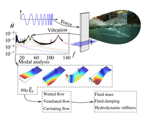
This two-part series aims to quantify the dynamic hydroelastic response of a surface-piercing hydrofoil in multiphase flows. The specific objectives of this installment (Part 2) are to (A) apply experimental modal analysis techniques for in situ measurement of the mode shapes, natural frequencies and damping ratios; (B) quantify the effect of immersion depth, flow speed and flow regime on the dynamical system parameters – namely the natural frequencies and damping ratios of the fluid–structure system; and (C) quantify the relative importance of fluid mass, fluid damping and hydrodynamic stiffness for the response of the coupled fluid–structure system. A secondary objective of this work is to demonstrate the effects that structural vibration can produce upon multiphase flow; to this end, we will show early results demonstrating that single-point excitation at specific resonances can be used to influence the size and stability of ventilated cavities in bi-stable flow conditions.
1.2 Overview
For a review of multiphase flows, including ventilation and cavitation, see Part 1. Section 2 summarizes the dynamical system model, describes classic modes of hydroelastic instability and summarizes the prior art. Much of the experimental approach was also described in Part 1; additional details are contained in § 3. The methodology of the modal parameter identification and results for natural frequencies and damping ratios are presented in § 4. Generalized force ratios are the topic of § 5. Conclusions, discussion and topics for future work are offered in § 6, including the effects of forced vibration on ventilated cavities.
2 Dynamic hydroelasticity in multiphase flows
In Part 1, a linearly elastic flexible body in a fluid was proposed to be described by the equations of motion,
 $$\begin{eqnarray}\unicode[STIX]{x1D648}_{\unicode[STIX]{x1D668}}\ddot{\boldsymbol{X}}+(\unicode[STIX]{x1D63E}_{\unicode[STIX]{x1D668}}+\unicode[STIX]{x1D642}_{\unicode[STIX]{x1D668}}\unicode[STIX]{x1D64E}^{D})\dot{\boldsymbol{X}}+\unicode[STIX]{x1D646}_{\unicode[STIX]{x1D668}}\boldsymbol{X}=\boldsymbol{F}_{\boldsymbol{ E}\boldsymbol{X}}+\boldsymbol{F}_{\boldsymbol{f}\boldsymbol{l}},\end{eqnarray}$$
 where  $\unicode[STIX]{x1D648}_{\unicode[STIX]{x1D668}}$,
  $\unicode[STIX]{x1D63E}_{\unicode[STIX]{x1D668}}$,
  $\unicode[STIX]{x1D642}_{\unicode[STIX]{x1D668}}$ and
  $\unicode[STIX]{x1D646}_{\unicode[STIX]{x1D668}}$ are respectively the structural mass, viscous and hysteretic structural damping and stiffness matrices. The scale matrix
  $\unicode[STIX]{x1D64E}^{D}$ is defined as
 $$\begin{eqnarray}\unicode[STIX]{x1D61A}_{ij}=\unicode[STIX]{x1D6FF}_{ij}\frac{|X_{i}|}{|\dot{X_{j}}|},\end{eqnarray}$$
 where  $\unicode[STIX]{x1D6FF}$ is the Kronecker delta. Here,
  $\unicode[STIX]{x1D64E}^{D}$ constrains the structural damping force to act proportionally to the displacement, but in phase with the velocity – a common model of hysteretic structural damping. The vector of nodal displacements
  $\boldsymbol{X}$ represents all spatial degrees of freedom,
  $\boldsymbol{F}_{\boldsymbol{E}\boldsymbol{X}}$ is a vector of external perturbations (steady and unsteady) and
  $\boldsymbol{F}_{\boldsymbol{f}\boldsymbol{l}}$ is the hydrodynamic force vector,
 $$\begin{eqnarray}\boldsymbol{F}_{\boldsymbol{f}\boldsymbol{l}}=\boldsymbol{F}_{\boldsymbol{s}\boldsymbol{f}\!,\boldsymbol{r}}+\boldsymbol{F}_{\boldsymbol{u}\boldsymbol{f}\!,\boldsymbol{r}}-(\unicode[STIX]{x1D648}_{\unicode[STIX]{x1D65B}}\ddot{\boldsymbol{X}}+\unicode[STIX]{x1D63E}_{\unicode[STIX]{x1D65B}}\dot{\boldsymbol{X}}+\unicode[STIX]{x1D646}_{\unicode[STIX]{x1D65B}}\boldsymbol{X}).\end{eqnarray}$$
The equations of motion may be re-cast as
 $$\begin{eqnarray}\displaystyle & & \displaystyle (\unicode[STIX]{x1D648}_{\unicode[STIX]{x1D668}}+\unicode[STIX]{x1D648}_{\unicode[STIX]{x1D65B}})\ddot{\boldsymbol{X}}+(\unicode[STIX]{x1D63E}_{\unicode[STIX]{x1D668}}+\unicode[STIX]{x1D63E}_{\unicode[STIX]{x1D65B}})\dot{\boldsymbol{X}}+\unicode[STIX]{x1D642}_{\unicode[STIX]{x1D668}}\unicode[STIX]{x1D64E}^{D}\dot{\boldsymbol{X}}+(\unicode[STIX]{x1D646}_{\unicode[STIX]{x1D668}}+\unicode[STIX]{x1D646}_{\unicode[STIX]{x1D65B}})\boldsymbol{X}\cdots \nonumber\\ \displaystyle & & \displaystyle \quad =\boldsymbol{F}_{\boldsymbol{E}\boldsymbol{X}}+\boldsymbol{F}_{\boldsymbol{s}\boldsymbol{f}\!,\boldsymbol{r}}+\boldsymbol{F}_{\boldsymbol{u}\boldsymbol{f}\!,\boldsymbol{r}}.\end{eqnarray}$$
 The fluid mass  $\unicode[STIX]{x1D648}_{\unicode[STIX]{x1D65B}}$, fluid damping
  $\unicode[STIX]{x1D63E}_{\unicode[STIX]{x1D65B}}$ and fluid hydrodynamic stiffness
  $\unicode[STIX]{x1D646}_{\unicode[STIX]{x1D65B}}$ account for the fluid forces respectively in phase with the acceleration, velocity and displacements of the flexible structure;
  $\boldsymbol{F}_{\boldsymbol{s}\boldsymbol{f}\!,\boldsymbol{r}}$ is the steady fluid load on an equivalent rigid lifting geometry at the same (undeformed) attitude as the flexible structure. For example, in Part 1,
  $\boldsymbol{F}_{\boldsymbol{s}\boldsymbol{f}\!,\boldsymbol{r}}$ represented the hydrodynamic lift and moment produced by an initial rigid-body angle of attack;
  $\boldsymbol{F}_{\boldsymbol{u}\boldsymbol{f}\!,\boldsymbol{r}}$ encompasses the various unsteady fluid force components acting on the equivalent rigid body (e.g. gusts, cavity shedding or vortex shedding). Finally, the fluid and structural matrices may be aggregated as,
 $$\begin{eqnarray}\left.\begin{array}{@{}c@{}}\unicode[STIX]{x1D648}=\unicode[STIX]{x1D648}_{\unicode[STIX]{x1D668}}+\unicode[STIX]{x1D648}_{\unicode[STIX]{x1D65B}},\\ \unicode[STIX]{x1D63E}=\unicode[STIX]{x1D63E}_{\unicode[STIX]{x1D668}}+\unicode[STIX]{x1D63E}_{\unicode[STIX]{x1D65B}},\\ \unicode[STIX]{x1D646}=\unicode[STIX]{x1D646}_{\unicode[STIX]{x1D668}}+\unicode[STIX]{x1D646}_{\unicode[STIX]{x1D65B}},\end{array}\right\}\end{eqnarray}$$
to write (2.4) in a consolidated form,
 $$\begin{eqnarray}\unicode[STIX]{x1D648}\ddot{\boldsymbol{X}}+(\unicode[STIX]{x1D63E}+\unicode[STIX]{x1D642}_{\unicode[STIX]{x1D668}}\unicode[STIX]{x1D64E}^{D})\dot{\boldsymbol{X}}+\unicode[STIX]{x1D646}\boldsymbol{X}=\boldsymbol{F}_{\boldsymbol{ E}\boldsymbol{X}}+\boldsymbol{F}_{\boldsymbol{s}\boldsymbol{f}\!,\boldsymbol{r}}+\boldsymbol{F}_{\boldsymbol{u}\boldsymbol{f}\!,\boldsymbol{r}}.\end{eqnarray}$$
2.1 Decoupled modal vibration
Diagonalization of (2.6) necessitates a series of simplifying assumptions, to be outlined in this section. Consider the unsteady solution only (or equivalently consider motion about the static equilibrium deflection) and assume that  $\boldsymbol{F}_{\boldsymbol{u}\boldsymbol{f}\!,\boldsymbol{r}}=\mathbf{0}$. Additionally, let the external force vector be of the form
  $\boldsymbol{F}_{\boldsymbol{E}\boldsymbol{X}}=\tilde{\boldsymbol{f}_{\boldsymbol{e}\boldsymbol{x}}}\text{e}^{st}$, with an associated response
  $\boldsymbol{X}=\tilde{\boldsymbol{X}_{\mathbf{0}}}\text{e}^{st}$, where the tilde
  $(\tilde{\text{ }})$ indicates a complex number and
  $s=\unicode[STIX]{x1D713}+\text{i}\unicode[STIX]{x1D714}$. Equation (2.4) then reduces to,
 $$\begin{eqnarray}(s^{2}\unicode[STIX]{x1D648}+s\unicode[STIX]{x1D63E}+\unicode[STIX]{x1D646}+s\unicode[STIX]{x1D642}_{\unicode[STIX]{x1D668}}\unicode[STIX]{x1D64E}^{D})\tilde{\boldsymbol{X}_{\boldsymbol{ 0}}}=\tilde{\boldsymbol{f}_{\boldsymbol{e}\boldsymbol{x}}},\end{eqnarray}$$
where the fluid and solid matrices have been combined as in (2.5).
Central to operational and modal vibration analysis is the frequency response function (FRF), which is a complex-valued representation of a system’s response to a given input,
 $$\begin{eqnarray}\unicode[STIX]{x1D60F}(\unicode[STIX]{x1D714})=\frac{\text{Output}(\unicode[STIX]{x1D714})}{\text{Input}(\unicode[STIX]{x1D714})}.\end{eqnarray}$$
 For a vibratory system with a single degree of freedom (SDOF), the FRF describes the response of the entire system. For multiple-degree-of-freedom (MDOF) systems with  $N$ degrees of freedom, the FRF takes the form of an
  $N\times N$ matrix, each containing a function
  $\unicode[STIX]{x1D60F}_{ij}(\unicode[STIX]{x1D714})$, that maps an input at the
  $j$th degree of freedom to an output at the
  $i$th degree of freedom of a system excited at an angular frequency of
  $\unicode[STIX]{x1D714}$. The name given to an FRF matrix depends upon the quantities defined as inputs and outputs, with a summary of common FRF types given in table 1.
Table 1. Common names of frequency response functions with input measurements  $X$ and output measurements
  $Y$.
$Y$.

The compliance FRF matrix, which requires that structural displacements be measured, is defined along the complex axis of the Laplace plane ( $s=\text{i}\unicode[STIX]{x1D714}$), so that
 $$\begin{eqnarray}\tilde{\unicode[STIX]{x1D643}}(\unicode[STIX]{x1D74E})\tilde{\boldsymbol{f}_{\boldsymbol{e}\boldsymbol{x}}}=\tilde{\boldsymbol{X}_{\mathbf{0}}}.\end{eqnarray}$$
By inspection, equation (2.7) shows that,
 $$\begin{eqnarray}\tilde{\unicode[STIX]{x1D643}}(\unicode[STIX]{x1D74E})^{-1}=-\unicode[STIX]{x1D714}^{2}\unicode[STIX]{x1D648}+\text{i}\unicode[STIX]{x1D714}\unicode[STIX]{x1D63E}+\unicode[STIX]{x1D646}+\text{i}\unicode[STIX]{x1D642}_{\unicode[STIX]{x1D668}}.\end{eqnarray}$$
 The fluid added mass, fluid damping and hydrodynamic stiffness matrices are, in general, dependent upon  $\unicode[STIX]{x1D714}$. The approach used in this work assumes that the frequency dependency in these matrices may be neglected through relatively narrow bands of the frequency domain surrounding a resonance. The same assumption is made regarding the structural damping matrix
  $\unicode[STIX]{x1D642}_{\unicode[STIX]{x1D668}}$, which is generally recognized as a frequency-dependent parameter. Collectively, these assumptions amount to a piecewise linearization of the dynamical system in the immediate neighbourhoods of points of interest – these points typically being modal peaks.
Fluid added mass, damping and stiffness matrices are additionally assumed to be invariant with respect to  $\ddot{\boldsymbol{X}}$,
  $\dot{\boldsymbol{X}}$ and
  $\boldsymbol{X}$, respectively – another linearization. Recent experiments by Phillips et al. (Reference Phillips, Cairns, Davis, Norman, Brandner, Pearce and Young2017) found nonlinearity in the effective damping ratio
  $\unicode[STIX]{x1D709}_{e}$ with respect to the amplitude of motion. This highlights the role that viscous and radiation damping – nonlinear effects – play in energy dissipation. However, the effect was limited to the first resonant mode. In the present work, this nonlinearity has been neglected – an assumption that may contribute to scatter in the experimental data to be shown.
Fluid loads can result in asymmetric system matrices – particularly on lifting surfaces, as in the case of the flow-induced bend–twist coupling shown in Part 1. Recent experimental and numerical results published by Young et al. (Reference Young, Garg, Brandner, Pearce, Butler, Clarke and Phillips2018a) showed a strong, but non-reciprocal, coupling between bending and twisting shape functions induced by the fluid loads. This was successfully modelled by an asymmetric coupling term in the hydrodynamic stiffness matrix  $\unicode[STIX]{x1D646}_{\unicode[STIX]{x1D65B}}$. Additionally, multiphase flows like vaporous cavitation have been shown by Benaouicha & Astolfi (Reference Benaouicha and Astolfi2012) to result in asymmetric added mass matrices. Maxwellian reciprocity of the effective system thus cannot be assumed – a fact that contributes to the complexity of the FSI response. In the asymmetric form, the equations of motion are almost directly analogous to the damped vibration of rotating structures, wherein gyroscopic follower forces can lead to systemic instabilities similar to the hydroelastic instabilities induced by fluid loading (Bucher & Ewins Reference Bucher and Ewins2001).
Both left and right eigenvectors are required to decouple the asymmetric equations of motion (Ma & Caughey Reference Ma and Caughey1995; Bucher & Ewins Reference Bucher and Ewins2001), where the right and left eigenvector matrices are respectively defined by the eigensolutions of the undamped free vibration problem (2.11a) and its adjoint (2.11b),
 $$\begin{eqnarray}\displaystyle & \displaystyle [\unicode[STIX]{x1D648}^{-1}\unicode[STIX]{x1D646}]\unicode[STIX]{x1D731}^{R}=\unicode[STIX]{x1D731}^{R}\unicode[STIX]{x1D740}^{D}, & \displaystyle\end{eqnarray}$$
 $$\begin{eqnarray}\displaystyle & \displaystyle \unicode[STIX]{x1D731}^{L}[\unicode[STIX]{x1D648}^{-1}\unicode[STIX]{x1D646}]=\unicode[STIX]{x1D740}^{D}\unicode[STIX]{x1D731}^{L}. & \displaystyle\end{eqnarray}$$
 The effective mass and effective stiffness matrices of the fluid–structure system are simultaneously diagonalizable by the left and right mass-orthonormalized eigenvectors (Caughey & O’Kelly Reference Caughey and O’Kelly1965), but the same cannot necessarily be said of the damping matrices  $\unicode[STIX]{x1D63E}$ and
  $\unicode[STIX]{x1D642}_{\unicode[STIX]{x1D668}}$. Thus, a final idealization must be proposed for these matrices. The structural and fluid damping matrices,
  $\unicode[STIX]{x1D63E}_{\unicode[STIX]{x1D668}}$,
  $\unicode[STIX]{x1D642}_{\unicode[STIX]{x1D668}}$ and
  $\unicode[STIX]{x1D63E}_{\unicode[STIX]{x1D65B}}$ are assumed to reside within the matrix space defined by the bases
  $\unicode[STIX]{x1D648}$ and
  $\unicode[STIX]{x1D646}$, such that each may be written as a linear combination of the mass and stiffness matrices. This is a form of damping known as proportional Rayleigh damping. Rayleigh damping is the classic example of general proportional damping (Rayleigh Reference Rayleigh1877), although formulations have also been proposed for more-general forms of proportional damping, based on Caughey series (Adhikari Reference Adhikari2006). However, this specific requirement of ‘proportional’ damping is rarely satisfied. For general damping matrices, the transformed damping matrix will possess off-diagonal elements, invalidating the modal decomposition proposed above and making experimental analysis both more computationally challenging and less physically intuitive. For the purposes of this work, we assume that the transformed damping matrix is diagonal, discarding small off-diagonal elements. This decoupling assumption is common in the literature (Ma & Caughey Reference Ma and Caughey1995) and generally well accepted when damping ratios are relatively small. With the decoupling assumption in place, the diagonalization of the effective system matrices becomes,
 $$\begin{eqnarray}\displaystyle & \displaystyle \unicode[STIX]{x1D731}^{L}\unicode[STIX]{x1D648}\unicode[STIX]{x1D731}^{R}=\unicode[STIX]{x1D644}^{D}, & \displaystyle\end{eqnarray}$$
 $$\begin{eqnarray}\displaystyle & \displaystyle \unicode[STIX]{x1D731}^{L}\unicode[STIX]{x1D646}\unicode[STIX]{x1D731}^{R}={\unicode[STIX]{x1D74E}_{\mathbf{0}}^{\mathbf{2}}}^{D}, & \displaystyle\end{eqnarray}$$
 $$\begin{eqnarray}\displaystyle & \displaystyle \unicode[STIX]{x1D731}^{L}\unicode[STIX]{x1D63E}\unicode[STIX]{x1D731}^{R}={\mathbf{2}\unicode[STIX]{x1D74E}_{\mathbf{0}}\unicode[STIX]{x1D743}}^{D}={\unicode[STIX]{x1D63E}^{\unicode[STIX]{x1D662}}}^{D}, & \displaystyle\end{eqnarray}$$
 $$\begin{eqnarray}\displaystyle & \displaystyle \unicode[STIX]{x1D731}^{L}\unicode[STIX]{x1D642}_{\unicode[STIX]{x1D64E}}\unicode[STIX]{x1D731}^{R}={\unicode[STIX]{x1D642}^{\unicode[STIX]{x1D662}}}^{D}={\boldsymbol{\unicode[STIX]{x1D702}}^{\boldsymbol{m}}}^{D}{\unicode[STIX]{x1D74E}_{\mathbf{0}}^{\mathbf{2}}}^{D}. & \displaystyle\end{eqnarray}$$
 ${\unicode[STIX]{x1D74E}_{\mathbf{0}}^{\mathbf{2}}}^{D}$,
  ${\unicode[STIX]{x1D63E}^{\unicode[STIX]{x1D662}}}^{D}$,
  $\unicode[STIX]{x1D743}^{D}$ and
  ${\boldsymbol{\unicode[STIX]{x1D702}}^{\boldsymbol{m}}}^{D}$ are respectively the diagonal matrices of squared undamped natural frequencies, viscous damping coefficients, critical damping ratios and hysteretic loss factors, where the superscript
  $m$ indicates a modal quantity and
  $\unicode[STIX]{x1D702}$ is known as the loss factor (Soroka Reference Soroka1949; Crandall Reference Crandall1970; Bert Reference Bert1973);
  $\unicode[STIX]{x1D714}_{0}$ is implicitly understood to be a modal quantity, so the superscript is omitted. Thus, the diagonalization of (2.10) with right and left eigenvectors yields,
  $$\begin{eqnarray}\unicode[STIX]{x1D731}^{L}\tilde{\unicode[STIX]{x1D643}}^{-1}(\unicode[STIX]{x1D714})\unicode[STIX]{x1D731}^{R}={\unicode[STIX]{x1D74E}_{\unicode[STIX]{x1D7EC}}^{\unicode[STIX]{x1D7EE}}}^{D}-\unicode[STIX]{x1D714}^{2}\unicode[STIX]{x1D644}^{D}+\text{i}\unicode[STIX]{x1D714}{\unicode[STIX]{x1D63E}^{\unicode[STIX]{x1D662}}}^{D}+\text{i}{\boldsymbol{\unicode[STIX]{x1D702}}^{\unicode[STIX]{x1D662}}}^{D}{\unicode[STIX]{x1D74E}_{\unicode[STIX]{x1D7EC}}^{\unicode[STIX]{x1D7EE}}}^{D},\end{eqnarray}$$
which leads to the matrix expression of the FRF,
 $$\begin{eqnarray}\tilde{\unicode[STIX]{x1D643}}(\unicode[STIX]{x1D74E})=\unicode[STIX]{x1D731}^{R}({\unicode[STIX]{x1D74E}_{\unicode[STIX]{x1D7EC}}^{\unicode[STIX]{x1D7EE}}}^{D}-\unicode[STIX]{x1D714}^{2}\unicode[STIX]{x1D644}^{D}+\text{i}\unicode[STIX]{x1D714}{\unicode[STIX]{x1D63E}^{\unicode[STIX]{x1D662}}}^{D}+\text{i}{\boldsymbol{\unicode[STIX]{x1D702}}^{\unicode[STIX]{x1D662}}}^{D}{\unicode[STIX]{x1D74E}_{\unicode[STIX]{x1D7EC}}^{\unicode[STIX]{x1D7EE}}}^{D})\unicode[STIX]{x1D731}^{L}.\end{eqnarray}$$
2.2 Hydroelastic instability
The linear dynamical system described by (2.4) and (2.6) is subject to two modes of instability: static divergence and dynamic flutter. The first occurs when the hydrodynamic stiffness negates the structural stiffness to make  $\unicode[STIX]{x1D646}$ singular, which leads to an undefined equilibrium condition where flow-induced disturbances can lead to unbounded deformations. As demonstrated in Part 1, off-diagonal elements in the hydrodynamic stiffness matrix
  $\unicode[STIX]{x1D646}_{\unicode[STIX]{x1D65B}}$ create flow-induced bend–twist coupling, which may be mitigated through the use of anisotropic material layups (Young et al. Reference Young, Garg, Brandner, Pearce, Butler, Clarke and Phillips2018a).
Dynamic flutter instability occurs when the at least one element of  ${\unicode[STIX]{x1D63E}^{\unicode[STIX]{x1D662}}}^{D}$ becomes zero or negative. The associated mode is known as the flutter mode and will experience undamped or growing oscillations. Flutter in coupled degrees of freedom classically occurs when two or more modal frequencies coalesce, with the shared frequency dubbed the ‘flutter frequency’, although flutter can occur prior to frequency coalescence, while the frequencies of the coupled modes are still approaching one another. The instability occurs when the effective modal damping of at least one of these coalescent modes becomes negative. This leads to an unbounded transfer of energy from a highly damped mode into the negatively damped flutter mode.
The topics of resonance (where a harmonic of the excitation force,  $\boldsymbol{F}_{\boldsymbol{E}\boldsymbol{X}}$, matches one of the system natural frequencies), flow-induced vibration (oscillatory response to harmonic content in
  $\boldsymbol{F}_{\boldsymbol{u}\boldsymbol{f}\!,\boldsymbol{r}}$) and lock in (resonance induced by harmonic
  $\boldsymbol{F}_{\boldsymbol{u}\boldsymbol{f}\!,\boldsymbol{r}}$) were introduced in Part 1. Multiphase flows lead to a secondary type of resonance, known as parametric resonance. Periodic cavity shedding acts as a source of flow-induced excitation on the one hand (Kaplan & Lehman Reference Kaplan and Lehman1966; Song Reference Song1969); on the other hand, the growth and collapse of the gaseous cavity periodically modifies the density and pressure fields around the body, while dissipating energy through turbulence and phase change. As a result, the system’s effective mass, damping and stiffness matrices modulate in time, as shown by Benaouicha & Astolfi (Reference Benaouicha and Astolfi2012), Akcabay et al. (Reference Akcabay, Chae, Young, Ducoin and Astolfi2014), Akcabay & Young (Reference Akcabay and Young2014, Reference Akcabay and Young2015). The frequency of modulation or one of its sub-harmonics can excite the natural frequency of the flexible body. Akcabay & Young (Reference Akcabay and Young2015) derived a SDOF model of parametric excitation and lock in using a van der Pol oscillator to model the modulation of system parameters with the cavity shedding frequency.
Physical instabilities are well documented and the accompanying theory is mature when the fluid in question is relatively light – i.e. aeroelasticity. However, as alluded to in Part 1, hydroelasticity poses unique challenges not present in aeroelastic analyses – e.g. increased viscous and inertial forces, the free surface, multiple phases, etc.
2.3 Prior art
Robust predictions of the fluid forces in multiphase flows are lacking; thus potentially dangerous instabilities are difficult or impossible to predict with the theoretical or numerical tools presently available. A recent review by Dehkharqani et al. (Reference Dehkharqani, Aidanpää, Engström and Cervantes2019) summarizes the challenges facing experimentalists and numerical modellers seeking to quantify fluid forces on vibrating hydraulic systems, with an emphasis on turbine runner blades. Abramson (Reference Abramson1969) succinctly summarized three characteristics of hydroelasticity that preclude the application of analyses from the more-mature field of aeroelasticity: the presence of a free surface, the presence of multiple phases (cavitation or ventilation) and low ratios of solid-to-fluid density (relative mass ratio). Indeed, for even fully submerged hydrofoils in uniform flow, no modifications to aeroelastic theory have been generally successful at capturing experimental results (Abramson Reference Abramson1969; Besch & Liu Reference Besch and Liu1971, Reference Besch and Liu1973; Chae Reference Chae2015). Experiments by Hilborne (Reference Hilborne1958) and Besch & Liu (Reference Besch and Liu1971, Reference Besch and Liu1973, Reference Besch and Liu1974) have explored and demonstrated, to varying degrees, the deficiencies in classical theory for reproducing the experimentally observed flutter boundaries. Besch & Liu (Reference Besch and Liu1973) specifically noted that predictions were extremely un-conservative at low value of  $\unicode[STIX]{x1D707}$. The same study led to the conclusion that flutter predictions were most deficient as a result of poor hydrodynamic damping estimates, and that theory was entirely unable to capture the onset of flutter in cavitating conditions or with modified boundary-layer profiles. More-detailed reviews of the hydrofoil flutter problem include Woolston & Castile (Reference Woolston and Castile1951), Abramson & Chu (Reference Abramson and Chu1959), Henry, Dugundji & Ashley (Reference Henry, Dugundji and Ashley1959), Abramson (Reference Abramson1969) and Chae, Akcabay & Young (Reference Chae, Akcabay and Young2013, Reference Chae, Akcabay and Young2017).
The problem of cavitation and ventilation on a lightweight, flexible surface-piercing hydrofoil is one possessing all three factors described by Abramson & Chu (Reference Abramson and Chu1959): a proximal free surface, multiple phases and a low mass ratio. Linear frequency-domain analysis is not able to accommodate these complex and nonlinear factors. Hence, most present-day researchers have turned to coupled time-domain simulations, which do not require the assumption of harmonic motion. These simulations recruit a variety of fluid and solid models, including 1-D lifting-line fluid model with 1-D beam-element finite-element analysis (FEA) (Ward, Harwood & Young Reference Ward, Harwood and Young2016, Reference Ward, Harwood and Young2018), boundary element method (BEM) fluid models coupled with 2-D and 3-D FEA solid models (Motley, Liu & Young Reference Motley, Liu and Young2009; Young Reference Young2010; Young, Baker & Motley Reference Young, Baker and Motley2010) and viscous computational fluid dynamics simulations coupled to FEA or reduced-order solid models (Chae et al. Reference Chae, Akcabay and Young2013, Reference Chae, Akcabay, Lelong, Jacques and Young2016; Akcabay & Young Reference Akcabay and Young2014, Reference Akcabay and Young2015). Even with the wealth of available tools, 3-D ventilating and cavitating flows around flexible bodies are governed by a panoply of complex physics that, considered individually, stress the capabilities of present numerical tools. Collectively, these phenomena have thus far defied simulation unless drastic simplifications are assumed.
Lindholm et al. (Reference Lindholm, Kana, Chu and Abramson1965) performed experiments on vibrating cantilevered plates partially immersed in water. They observed that natural frequencies decreased with immersion in the water and demonstrated that the reduction was caused by fluid added mass. The added mass coefficient, denoting the ratio of fluid mass to generalized solid mass for a given mode, was modelled with reasonable fidelity using plate theory with empirical corrections. Added-mass correlations were sought by De La Torre et al. (Reference De La Torre, Escaler, Egusquiza and Farhat2013) for cavitating flows. The added mass coefficient was linearly correlated with the entrained mass – a measure of the fluid mass contained in the normalized swept volume of a given mode. The added-mass coefficients were also shown to decrease with increasing cavity size. All data derived from mode shapes relied upon FEA simulations, rather than experimental data. The study neglected the effects of fluid hydrodynamic stiffness; all changes in resonant frequencies were attributed to changing mass. This is not strictly true because, as demonstrated in Part 1 of this paper and by Harwood (Reference Harwood2016) and Harwood et al. (Reference Harwood, Ward, Young and Ceccio2016b, Reference Harwood, Ward, Felli, Falchi, Ceccio and Young2017), the fluid hydrodynamic stiffness – at least for an assumed twisting mode – is negative and scales with the squared velocity.
In discussing modal characteristics across different system conditions (e.g. varying flow regimes), one must remain cognizant that the natural frequencies and critical damping ratios are normalized by quantities that, themselves, change with the conditions of the system (discussed further in § 5). Blake & Maga (Reference Blake and Maga1975), Reese (Reference Reese2010) have addressed the changing denominators of modal parameters by re-normalizing those identified parameters by shared reference values. Damping ratios, for example, were supplanted by loss factors, which were then re-normalized to a common modal mass so that addition and subtraction of loss factors across changing flow regimes was permissible. By this method, viscous and hydrodynamic damping were separated from the total damping and from one another by sequentially testing the vibrating structure in air, in still water and in moving water. Blake & Maga (Reference Blake and Maga1975) found that the loss factor of a cantilever increased when immersed in water and increased further when that water began to flow. This latter ‘hydrodynamic’ damping was found to increase monotonically with increasing flow speed, reaching values approximately 10 times greater than the loss factors in still water.
Generalized fluid and structural forces have been used with an assumed-mode analysis by Chae et al. (Reference Chae, Akcabay and Young2013), Chae (Reference Chae2015), Chae et al. (Reference Chae, Akcabay, Lelong, Jacques and Young2016), Young et al. (Reference Young, Garg, Brandner, Pearce, Butler, Clarke and Phillips2018a,Reference Young, Garg, Brandner, Pearce, Butler, Clarke and Phillipsb) to model the dynamic response of wetted and cavitating hydrofoils. In this method, a two-dimensional, 2-degree-of-freedom (2D-2DOF) model was used to predict sectional hydrodynamic loads, which were then generalized by integration along spanwise bending and twisting shape functions.
3 Experimental approach
The experiments yielding data for this work were previously described in Part 1, and will be only briefly summarized herein. Detailed descriptions are reserved for instruments not previously described.
3.1 Surface-piercing hydrofoil
A single flexible hydrofoil (referred to in Part 1 of this paper as hydrofoil Model 2) was used for the present work. It was configured as a vertical strut having a rectangular plan form with a span of 91.4 cm (36 in.) and a chord length of 28.58 cm (11.25 in.). The hydrofoil was constructed of Type 1 PVC (known also as rigid PVC), which has a density of  $1486~\text{kg}~\text{m}^{-3}$, a Young’s modulus of
  $E=3.36$ GPa, a shear modulus of
  $G=1.2~\text{GPa}$ and a Poisson ratio of 0.4. The foil section was a semi-ogive similar to that of Harwood, Young & Ceccio (Reference Harwood, Young and Ceccio2016c), with the only difference being a thin strip of aluminium affixed to the trailing edge to increase the bending strength of the section. The aluminium strip was 2.8 cm wide by 0.64 cm thick (1.1 in. by 0.25 in.). A cross-section of the foil is shown in figure 1, with the locations of the centre of mass, the shear centre and the assumed centre of pressure (although this last point moves as a function of the flow regime).

Figure 1. Section geometry of flexible hydrofoil. The section shape is identical to that of Harwood et al. (Reference Harwood, Young and Ceccio2016c), with the exceptions of interior channels machined along the centre plane and the addition of an aluminium strip along the trailing edge (TE) for structural reinforcement. The aluminium strip was attached with a combination machine screws and adhesive. The coordinate system is located at the midpoint of the un-appended chord length of 27.9 cm.
Figure 2 depicts the mounting arrangement, coordinate system and relevant variables. As in Part 1, the hydrofoil was mounted vertically with the tip piercing the surface of the water to a depth  $h$. The tang of the hydrofoil was clamped to achieve a cantilever configuration. The hydrofoil was yawed about its
  $Z$-axis to set the angle of attack with respect to the incoming flow.

Figure 2. (a) Depiction of experimental coordinate system and test variables.  $U$ is the flow speed,
  $\unicode[STIX]{x1D6FC}$ is the yaw angle (angle of attack),
  $h$ is the immersion of the free tip beneath the undisturbed free surface,
  $c$ is the foil chord and
  $S$ is the cantilevered span of the hydrofoil.
  $z^{\prime }$ is defined as the vertical distance beneath the undisturbed free surface, such that
  $z^{\prime }=h$ at the free tip. (b) Diagram of experimental instrumentation, described in § 3.4.
3.2 Test environment 1: free-surface cavitation channel
All hydrodynamic testing was performed in the free-surface, variable-pressure recirculating water channel operated by the National Research Council – Institute of Marine Engineering (CNR INM) at its campus in Rome, Italy. The channel has a test section measuring  $10~\text{m}\times 3.6~\text{m}\times 3~\text{m}$ (
 $L\times W\times D$) and operates with a water depth of 2.25 m. Free-surface conditioning is achieved by an inverted backward step at the entrance to the test section. The hydrofoil was mounted approximately 2.3 m downstream of the step, at the centre of the test section, suspended from transverse steel rails, as shown in figure 3.
The channel has a maximum flow speed of  $5~\text{m}~\text{s}^{-1}$ with an uncertainty on the mean velocity of approximately 1.5 %. The hydrofoil was tested at speeds between
  $1~\text{m}~\text{s}^{-1}$ and
  $4.2~\text{m}~\text{s}^{-1}$, with corresponding depth-based Froude numbers between 0.6 and 2.54. The depth-based Froude number is defined as
 $$\begin{eqnarray}Fn_{h}=\frac{U}{\sqrt{gh}}.\end{eqnarray}$$
 A flow quality survey (described in Part 1) showed that a mean cross-channel flow occurs at all speeds, augmenting the hydrofoil’s angle of attack by approximately  $2^{\circ }$, with a standard deviation of approximately
  $2^{\circ }$.

Figure 3. Views of the experimental set-up in the CNR INM cavitation channel. (a) View from control room (viewed along negative  $Y$ direction). (b) View from inside of the cavitation channel (perspective from (
 $-X$,
$-X$,  $-Y$,
$-Y$,  $+Z$) octant).
3.3 Test environment 2: vibration test frame
Vibration testing of the hydrofoil in a quiescent fluid was conducted using a ground-fixed steel frame that suspended the hydrofoil in a water-filled drum with a capacity of 246 l (65 gallons). The set-up, depicted in figure 4, was described by Harwood et al. (Reference Harwood, Stankovich, Young and Ceccio2016a). The immersion depth of the hydrofoil was varied by filling and draining the drum. The limited capacity of the drum was determined not to affect the measured vibration response appreciably (see § 4).

Figure 4. Free-standing test frame used to measure the vibratory response of the hydrofoil at varying values of the immersed aspect ratio  $AR_{h}$ in quiescent water. Operator shown for scale.
3.4 Instrumentation
Forces were measured using an ATI Omega-190 6-degree-of-freedom load cell, with a multi-axis uncertainty of approximately 2.6 %. Measurements of the flexible hydrofoil deflections were made with custom shape-sensing spars, detailed in Di Napoli et al. (Reference Di Napoli, Young, Ceccio and Harwood2019). Two spars were used to measure lateral deflections along non-co-linear paths along the foil’s span, which were then cast as bending and torsional deflection of the hydrofoil’s elastic axis. From Di Napoli et al. (Reference Di Napoli, Young, Ceccio and Harwood2019), the measurement uncertainties at the free tip of the hydrofoil under static loading are 2.1 % (proportional) in bending and  $0.49^{\circ }$ (absolute) in twisting within the calibrated range of
  $\pm 8~\text{cm}$ in bending (9 % of the hydrofoil span) and
  $\pm 5^{\circ }$ in twisting.
The pressure inside the test section was measured with a dry pressure transducer with an uncertainty of  $\pm 5$ mbar, and verified with a mercury manometer with an estimated uncertainty of
  $\pm 1$ mbar. Single-axis charge-type accelerometers (PCB Piezotronics® model 357B06) were affixed to the end of each shape-sensing spar to provide additional motion data near the tip of the hydrofoil for the ensuing modal analysis. Additional single-axis accelerometers manufactured by PCB® were mounted to the transverse steel beams of the test section (see figure 3) to monitor parasitic vibration of the test facility. A modified version of the air-injection system used by Harwood et al. (Reference Harwood, Young and Ceccio2016c) was used to trigger ventilation in the bi-stable range of flow conditions by creating turbulent, bubbly flow at the leading edge of the hydrofoil.
High-speed video was recorded in test environment 1 using two Photron® brand high-speed cameras (FASTCAM® SA-Series) aimed through windows in the test section – one aimed horizontally at the submerged suction surface and one aimed vertically upward at the foil’s free tip. Both cameras acquired frames in 12-bit grey scale at a resolution of  $1024\times 512$ pixels and a rate of
  $500$ frames per second.
3.4.1 Shaker excitation and drive-point measurements
A linear shaker motor (model 2007E ‘mini-shaker’, manufactured by The Modal Shop®) was attached to the suction side of the hydrofoil above the still waterline to provide a harmonic excitation force at a commanded frequency. Forces and accelerations at the drive point were measured with a PCB Piezotronics® impedance head (model 288D01). Excitation signals were generated as sinusoid waveforms from a Stanford Research Systems® SR830 lock-in amplifier, phase locked to a TTL pulse train generated by the data collection computer. The excitation signal was a discretely stepped logarithmic sweep, wherein each commanded frequency was held constant for an integer number of cycles  $N_{C}$, as shown in figure 5. Sweeps were conducted over a frequency band sufficient to excite the first five resonant modes (between 2 Hz and 140 Hz or more) with frequency step sizes of 0.1 Hz to 0.3 Hz. Convergence testing demonstrated that modal parameters did not vary strongly with the number of periods for
  $N_{C}\geqslant 5$, and all reported trials were conducted with
  $N_{C}\geqslant 10$.
During vibration testing, runs containing non-stationary responses, such as formation or elimination of a ventilated cavity, were voided and repeated until a complete frequency sweep was attained in an unchanging flow regime. Other sources of non-stationarity, such as inflow fluctuations or partial cavity shedding were an unavoidable source of error. In particular, fluctuations in cross-flow angle were observed to occur at frequencies below 10 Hz, introducing some spurious spectral content, discussed further in § 4.2. A zero-phase-shift digital high-pass filter was used during post-processing to remove mean and slowly varying forces and deflections below 2 Hz. As mentioned in Part 1, some unavoidable sensor drift was observed, particularly in the shape-sensing spars. Regular bias measurements and filtering ensured that the slow drift had no effect upon the higher-frequency dynamics discussed in this work.

Figure 5. Typical shaker motor excitation signal with  $N_{C}=25$ complete periods at each frequency.
4 Identification of modal parameters
In this section, the experimental modal analysis (EMA) of the hydrofoil’s FSI response will be detailed, followed by quantification of FRFs, mode shapes, resonant frequencies and effective damping ratios.
4.1 Experimental modal analysis
Each individual FRF in the matrix  $\tilde{\unicode[STIX]{x1D643}}$ may be written as for a single degree of freedom, which follows from (2.14),
 $$\begin{eqnarray}\tilde{H}_{jk}(\unicode[STIX]{x1D714})=\mathop{\sum }_{n=1}^{N_{DOF}}\frac{\unicode[STIX]{x1D6F7}_{jn}^{R}\unicode[STIX]{x1D6F7}_{kn}^{L}}{\unicode[STIX]{x1D714}_{0,n}^{2}-\unicode[STIX]{x1D714}^{2}+\text{i}(\unicode[STIX]{x1D714}_{0}^{2}\unicode[STIX]{x1D702}_{n}+2\unicode[STIX]{x1D714}\unicode[STIX]{x1D714}_{0,n}\unicode[STIX]{x1D709}_{n})},\end{eqnarray}$$
 where  $k$ and
  $j$ are the respective indices of the excitation and response degrees of freedom. Here,
  $N_{DOF}$ denotes the number of instrumented degrees of freedom, and hence the number of modes that can be resolved. Alternatively, the summation may be performed over some truncated number of modes,
  $N<N_{DOF}$, in which case (4.1) describes a reduced-order model of the dynamical system. In the immediate neighbourhood of each resonance (i.e. when
  $\unicode[STIX]{x1D714}\approx \unicode[STIX]{x1D714}_{0,n}$), the two damping parameters (
 $\unicode[STIX]{x1D702}_{n}$ and
  $\unicode[STIX]{x1D709}_{n}$) are combined into an effective viscous damping coefficient
  $\unicode[STIX]{x1D709}_{e,n}=\unicode[STIX]{x1D709}_{n}+\unicode[STIX]{x1D702}_{n}/2$, yielding as the modal superposition equation,
 $$\begin{eqnarray}\tilde{H}_{jk}(\unicode[STIX]{x1D714})=\mathop{\sum }_{n=1}^{N_{DOF}}\frac{\unicode[STIX]{x1D6F7}_{jn}^{R}\unicode[STIX]{x1D6F7}_{kn}^{L}}{\unicode[STIX]{x1D714}_{0,n}^{2}-\unicode[STIX]{x1D714}^{2}+\text{i}2\unicode[STIX]{x1D714}\unicode[STIX]{x1D714}_{0,n}\unicode[STIX]{x1D709}_{e,n}}.\end{eqnarray}$$
 In the present work, FRF matrices were estimated by the  $H_{1}$ estimator, defined as,
 $$\begin{eqnarray}\tilde{H}_{1,ij}=\frac{XPS(F_{i},X_{j})}{APS(F_{i})},\end{eqnarray}$$
 where  $F_{i}$ is an input at degree of freedom
  $i$ and
  $X_{j}$ is the output at degree of freedom
  $j$. For all cases, auto-power spectra (APS) and cross-power spectra (XPS) were smoothed using between 8 and 32 segments with Hanning windows and a
  $75\,\%$ overlap. Other estimators were tried in an effort to reduce the effects of measurement noise in the input and output – namely the
  $H_{2}$,
  $H_{3}$ and hybrid
  $H_{V}$ estimators (Ewins Reference Ewins2000), but they produced no appreciable difference in the extracted modal parameters. Hence, the subscript
  $1$ will be dropped and the FRF will be denoted simply by
  $\tilde{H}$.
The compliance FRF  $\tilde{\unicode[STIX]{x1D643}}^{\unicode[STIX]{x1D658}\unicode[STIX]{x1D664}\unicode[STIX]{x1D662}\unicode[STIX]{x1D665}}$ was determined by using inferred deflections as the system output. The structural deflections of the hydrofoil were reconstructed at ten uniformly distributed spanwise locations along the leading edge (LE) and ten points on the trailing edge (TE). Excluding the root, at which point motion is identically zero, this yields a row of the compliance FRF matrix,
  $\tilde{\boldsymbol{H}}^{\boldsymbol{c}\boldsymbol{o}\boldsymbol{m}\boldsymbol{p}}\in \mathbb{C}^{1\times 18}$, at each frequency. Note that eight strain gauges were installed, so
  $\text{rank}\;(\tilde{\unicode[STIX]{x1D643}}^{\unicode[STIX]{x1D658}\unicode[STIX]{x1D664}\unicode[STIX]{x1D662}\unicode[STIX]{x1D665}})=8$, yielding only eight independent estimates of the modal parameters for each mode. The over-fitting, however, ensured that if a reconstruction point fell on or near a node line – and consequently produced a spurious identification – it could be rejected as an outlier whilst retaining eight independent estimates. The inertance FRF was obtained by taking the accelerations measured at the tip of each spar as outputs, yielding a row of the inertance matrix,
  $\tilde{\boldsymbol{H}}^{\boldsymbol{i}\boldsymbol{n}\boldsymbol{e}\boldsymbol{r}\boldsymbol{t}}\in \mathbb{R}^{1\times 2}$.
Each FRF in (4.2) can be fitted as a ratio of polynomials on  $s$ (Richardson & Formenti Reference Richardson and Formenti1982) to yield the rational fraction polynomial (RFP) transfer function of the system – written in the complex
  $s$ plane,
 $$\begin{eqnarray}\tilde{\unicode[STIX]{x1D643}}(\unicode[STIX]{x1D668})=\frac{\displaystyle \mathop{\sum }_{m=0}^{M_{n}}b_{m}s^{m}}{\displaystyle \mathop{\sum }_{n=0}^{N_{d}}a_{n}s^{n}},\end{eqnarray}$$
 where  $M_{n}$ and
  $N_{d}$ are respectively the orders of the numerator and denominator polynomials. For a linear, time-invariant system, the transfer function will possess Hermitian symmetry – such that its poles exist in complex conjugate pairs – which permits a partial-fraction expansion of (4.4) to yield,
 $$\begin{eqnarray}\tilde{\unicode[STIX]{x1D643}}=\mathop{\sum }_{n=1}^{N_{d}/2}\left(\frac{\tilde{\unicode[STIX]{x1D64D}}_{\unicode[STIX]{x1D663}}}{s-\tilde{p}_{n}}+\frac{{\tilde{\unicode[STIX]{x1D64D}}_{\unicode[STIX]{x1D663}}}^{\ast }}{s-\tilde{p}_{n}^{\ast }}\right).\end{eqnarray}$$
 Here,  $\tilde{\unicode[STIX]{x1D64D}}_{\unicode[STIX]{x1D663}}$ and
  ${\tilde{\unicode[STIX]{x1D64D}}_{\unicode[STIX]{x1D663}}}^{\ast }$ are the residue matrix and its complex conjugate, respectively, of the
  $n$th mode. Similarly,
  $\tilde{p}_{n}$ and
  $\tilde{p}_{n}^{\ast }$ are the
  $n$th complex pole and its conjugate. For a system of
  $N_{DOF}$ degrees of freedom,
  $N_{d}=2N_{DOF}$ to include the conjugate pairs of the
  $N_{DOF}$ modes of the vibratory system. Recalling that
  $s=\unicode[STIX]{x1D70E}+\text{i}\unicode[STIX]{x1D714}$, each pole yields,
 $$\begin{eqnarray}\displaystyle \tilde{p}_{n} & = & \displaystyle \unicode[STIX]{x1D713}_{n}+\text{i}\unicode[STIX]{x1D714}_{n}\nonumber\\ \displaystyle & = & \displaystyle \unicode[STIX]{x1D714}_{0,n}\unicode[STIX]{x1D709}_{e,n}+\text{i}\unicode[STIX]{x1D714}_{0,n}\sqrt{1-\unicode[STIX]{x1D709}_{e,n}^{2}}.\end{eqnarray}$$
The undamped resonant frequency, damped resonant frequency and damping ratio are then given by the following expressions:
 $$\begin{eqnarray}\displaystyle & \displaystyle \unicode[STIX]{x1D714}_{0,n}=\Vert \tilde{p}_{n}\Vert \quad \text{Undamped Natural Frequency}, & \displaystyle\end{eqnarray}$$
 $$\begin{eqnarray}\displaystyle & \displaystyle \unicode[STIX]{x1D714}_{n}=\text{Im}(\tilde{p}_{n})\quad \text{Damped Natural Frequency}, & \displaystyle\end{eqnarray}$$
 $$\begin{eqnarray}\displaystyle & \displaystyle \unicode[STIX]{x1D709}_{e,n}=\frac{\text{Re}(\tilde{p}_{n})}{\Vert \tilde{p}_{n}\Vert }\quad \text{Modal Damping Ratio}. & \displaystyle\end{eqnarray}$$
 During analysis, spectra were analysed interactively. Regions of the FRF were selected graphically, with  $N$ denoting the number of selected resonances. The number of in-band and out-of-band resonances were specified to determine the RFP polynomial orders
  $M_{n},N_{d}$. Transfer-function coefficients, poles, residues and direct terms were found by sequential application of MATLAB® functions invfreqs and residue. Hermitian symmetry was ensured by reflecting the experimentally measured
  $\tilde{\unicode[STIX]{x1D643}}$ about the origin and imposing anti-symmetry on the imaginary component, thus ensuring that poles and residues were returned as conjugate pairs. For each of the
  $N$ identified poles of the transfer function, a vector of resonant frequencies and viscous damping ratios can be obtained, respectively,
  $\unicode[STIX]{x1D74E}_{\mathbf{0}}\in \mathbb{R}^{N_{DOF}\times 1}$ and
  $\unicode[STIX]{x1D743}_{\boldsymbol{e}}\in \mathbb{R}^{N_{DOF}\times 1}$. Estimates of global parameters
  $\unicode[STIX]{x1D709}_{e,n}$ and
  $\unicode[STIX]{x1D714}_{0,n}$ for each mode were aggregated from the inertance and compliance FRFs. Spurious estimates were first removed visually, and the remaining samples were subjected to an iterative Grubbs test (Grubbs Reference Grubbs1969) with a 95 % confidence interval to remove statistical outliers. Outlier rejection was performed with the MATLAB script deleteouliers (Shoelson Reference Shoelson2011). Means and standard deviations were computed for
  $\unicode[STIX]{x1D714}_{0,n}$,
  $\unicode[STIX]{x1D709}_{e,n}$ from the remaining samples.
Comparison of (4.1) and (4.5) reveals that the residue matrix of the  $n$th mode is related to the outer product of the
  $n$th mode shape from the right and left eigenvectors as,
 $$\begin{eqnarray}\tilde{\unicode[STIX]{x1D64D}}_{\unicode[STIX]{x1D663}}=\tilde{q}_{n}\unicode[STIX]{x1D731}_{\boldsymbol{n}}^{\boldsymbol{R}}\unicode[STIX]{x1D731}_{\boldsymbol{n}}^{\boldsymbol{L}},\end{eqnarray}$$
 where  $q_{n}$ is a non-unique scale factor. As a result, any row or column of the residue matrix contains a re-scaled mode shape. If a single modal contribution is considered (mode
  $n$), then when
  $\unicode[STIX]{x1D714}=\unicode[STIX]{x1D714}_{0,n}$, the real part of (4.2) is nullified, leaving an imaginary component only. Finally, a straightforward (but laborious) expansion of the
  $n$th term of (4.5) shows that, if (4.5) is to satisfy the same condition at the undamped resonant frequency, then the real part of the residue matrix
  $\tilde{\unicode[STIX]{x1D64D}}_{\unicode[STIX]{x1D663}}$ must be zero. From these considerations, an unscaled mode shape – or more precisely, a mode shape with an unknown scaling factor – denoted
  $\hat{\unicode[STIX]{x1D731}}_{\boldsymbol{n}}$, may be obtained from any row or column of the residue matrix (depending upon the number of inputs and outputs used to collect data) as,
 $$\begin{eqnarray}\hat{\unicode[STIX]{x1D731}}_{\boldsymbol{n}}=\text{Im}\{\boldsymbol{R}_{\boldsymbol{n}}\},\end{eqnarray}$$
 where  $\boldsymbol{R}_{\boldsymbol{n}}$ is any column or row of
  $\tilde{\unicode[STIX]{x1D64D}}_{\unicode[STIX]{x1D663}}$, recast as a column vector. It should be noted, as well, that the unscaled mode shape
  $\hat{\unicode[STIX]{x1D731}}_{\boldsymbol{n}}$ comes from a column of
  $\unicode[STIX]{x1D731}^{R}$ or a row of
  $\unicode[STIX]{x1D731}^{L}$. In this work, a single column vector of
  $\tilde{\unicode[STIX]{x1D64D}}_{\unicode[STIX]{x1D663}}$ was obtained (single excitation point with distributed response measurements), so the former is true.
It is important to note that, while the FRF (and its transfer function representation) is an  $N_{DOF}\times N_{DOF}$ matrix of residues, the denominator of each modal contribution is a complex scalar. The interpretation of this fact is important: the resonant frequency and damping (respectively
  $\unicode[STIX]{x1D714}_{0,n}$ and
  $\unicode[STIX]{x1D709}_{e,n}$) of each mode
  $n$ are global parameters that do not vary with the location of the input or output. As a result, each FRF measurement in the FRF matrix should contain identical modal parameters. Thus, to improve the estimates of mode shapes during data analysis, the global pole location was prescribed from the mean damping ratio and undamped resonant frequency, and the numerator of (4.4) was re-fitted to find residue matrices consistent with the system’s global resonances – an iterative approach recommended by Richardson & Formenti (Reference Richardson and Formenti1982).
Supplementary data available online at https://doi.org/10.1017/jfm.2019.871 include tabulated modal parameters for each unique combination of  $Fn_{h}$,
  $AR_{h}$, flow regime, test facility and mode.
4.2 Frequency response functions and mode shapes in various flow regimes
To introduce the ways in which the vibratory response of the hydrofoil changes as a function of flow conditions, this section is dedicated to a mostly qualitative comparison of five example trials, conducted at the CNR INM cavitation channel; quantitative examinations of specific variations in immersion depth, flow regime, Froude number, etc. follow in later sections. The cases selected typify the hydrofoil’s operating regimes, defined as follows:
(i) Dry conditions.
(ii) Partial immersion (
 $AR_{h}=1.0$) in still water.
(iii) Partial immersion (
$AR_{h}=1.0$) at forward speed ($Fn_{h}=1.5$; $U=2.48~\text{m}~\text{s}^{-1}$) in FW flow at $\unicode[STIX]{x1D6FC}=0^{\circ }$.(iv) Partial immersion (
$AR_{h}=1.0$) at forward speed ($Fn_{h}=1.5$; $U=2.48~\text{m}~\text{s}^{-1}$) in FV flow at $\unicode[STIX]{x1D6FC}=10^{\circ }$.(v) Partial immersion (
$AR_{h}=1.0$) at forward speed ($Fn_{h}=1.5$; $U=2.48~\text{m}~\text{s}^{-1}$) in PC flow at $\unicode[STIX]{x1D6FC}=10^{\circ }$; $\unicode[STIX]{x1D70E}_{v}=0.85$.


4.2.1 Dry conditions
The magnitude of the compliance FRF, averaged across all degrees of freedom and decomposed into the contributions from each mode (modal participation factors), is shown in figure 6. Modes 1, 2, 3 and 5 are observed experimentally. The modal frequencies predicted with the FEA model are overlaid and labelled as vertical lines. At specific frequencies, components of the mounting structure or facility resonated, creating artificial peaks in the measured FRF. These are designated in the figure as ‘contaminants’. Contaminants were identified as frequency peaks that remained independent of the partial immersion of the hydrofoil. The primary contaminant is thought to be resonance of the bracket used to attach the shaker motor to the hydrofoil, which occurs between 50 Hz and 55 Hz. Over the course of testing, gradual loosening of threaded braces on the bracket caused a slow decreasing trend in its resonant frequencies. A second significant source of contamination occurred with vibration of the transverse rails (shown in figure 3), to which the hydrofoil set-up was attached. The rails, which acted as simply supported beams, began vibrating in a fundamental vertical mode at 38 Hz (confirmed by accelerometer measurements of the rails). Some additional contamination of the spectrum near  $f=100~\text{Hz}$ is due to another resonant mode of the cavitation channel structure, and is compounded by the second harmonic of the AC line noise at 50 Hz. The thick grey line plotted over the measured FRF represents principal-component reconstruction of the compliance FRF, yielded by applying summing equation (4.1) over the four resonances of interest (omitting the contaminants). Finally, it should be noted that the peaks of the individual modes in the FRF are indicative of the damped natural frequencies of the respective modes, which are slightly smaller than the undamped experimental frequencies listed in table 2.

Figure 6. FRF decomposition for the hydrofoil in dry conditions. The vertical grey lines indicate modal frequencies predicted by the FEA model. Data collected for 1660 s at 500 Hz. Contaminant modes include vibration of the shaker motor mount at approximately 50 Hz, facility modes at 38 Hz and approximately 100 Hz and AC line noise and harmonics thereof at multiples of 50 Hz.
An FEA modal analysis was performed in ANSYS Mechanical®. The details of the model are contained in appendix A. The comparison between the modes predicted by the FEA model and those estimated by EMA are shown in tabular form in table 2 and the resulting mode shapes are compared in figure 7. The agreement is generally good, although FEA tends to over-predict the frequencies of higher modes. The FEA model accounted for the compliance of the load cell and the root clamp, but there remains some small compliance in the vibration test structure to which the load cell is mounted that departs from the simulated assumption of a perfect clamp at the base of the load cell. Additionally, some frictional losses are present in bolted connections that are not captured by the undamped modal analysis. Both of these observations contribute to the differences between FEA and EMA. Nevertheless, modal frequencies are in close agreement, with a maximum error of 6.8 %. The associated mode shapes are dimensionless, so apparent differences between the magnitude of simulated and experimental modes are of no physical significance. The number and orientation of nodal lines are in good agreement, with the exception of the third ordered mode (X-Bend 2). The nodal line for the third mode lies at a different angle than that of the predicted mode shape. The contaminant mode attributed to the shaker motor mounting bracket is a dominant component in the FRF between modes 2 and 3, while mode 3 appears significantly less energetic. The proximity of the contaminant mode is therefore hypothesized to cause a flawed mode shape estimation. Fortunately, the global frequency and damping ratio estimates are less affected by the nearby contaminant than is the residue matrix, so the other modal parameters are thought to remain valid.
Table 2. Comparison of undamped natural frequencies (  $f_{0}$) and mode shape descriptions between FEA and EMA. Note that mode 4 (lead lag) is not observed experimentally because the shape-sensing spars are designed to measure lateral bending strains only.


Figure 7. Comparison of in vacuo mode shapes predicted by FEA model and extracted by EMA. The experimental mode shapes have been placed in the same orientation as the FEA figures. Qualitative agreements are good, though the nodal line of the X-Bend 2 mode does not match between the experiment and the simulation. Experimental modes 1, 2, 3 and 5 were measured in the CNR INM channel in dry conditions, using a frequency sweep with a step size of 0.05 Hz and  $N_{C}=15$ cycles at each discrete frequency. Mode 6 was measured on the vibration frame at the University of Michigan, using a continuous linear frequency sweep.
4.2.2 Effects of partial immersion in still water
In figure 8, the resonant frequencies of all modes at  $AR_{h}=1.0$ in still water decrease compared to the dry condition. This reduction occurs as a result of increased fluid added mass, which causes inertial resistance to the motion of the hydrofoil. The contaminating modes, however, remain fixed (one of the ways in which the contaminants were identified and separated from the modes of interest). Those contaminant modes are better separated from the modes of interest in quiescent water, particularly near the third (X-Bend 2
  $+$ Twist) mode. No differences are immediately obvious in the widths of the individual peaks, compared to figure 6, which suggests that the damping ratio (
 $\unicode[STIX]{x1D709}_{e}$) is not strongly affected by partial immersion in quiescent liquid.

Figure 8. FRF decomposition for the hydrofoil in still water  $\unicode[STIX]{x1D6FC}=10^{\circ }$;
  $Fn_{h}=0$;
  $AR_{h}=1.0$. Data collected for 4500 s at 500 Hz.
4.2.3 Effects of forward speed and flow regime
Figure 9 depicts the FRFs for the hydrofoil in typical FW, FV and PC flows alongside the FRF for a quiescent fluid. The top plot contains the experimental FRF, while the bottom plot contains the FRF curve fits, reconstructed from the identified modes; individual fitted modes are omitted for clarity. The spectra for each of the flow regimes with individual modal contributions are shown in figures 25–27 in appendix B.

Figure 9. FRFs of the flexible hydrofoil in quiescent water, FW flow, FV flow and PC flow. The top plot depicts the (smoothed) experimental FRFs. The lower plot depicts the de-noised FRFs synthesized from the fitted modes, excluding contaminant modes. Inset photographs show the flow pattern in each flow regime. Note, in particular, the photographs from two instants in PC flow that demonstrate the unsteadiness in the leading edge cavity. All data were collected at a sampling rate of 500 Hz. Recording durations were as follows. FW flow: 520 s. FV flow: 1900 s. PC flow: 930 s.
In FW flow with forward speed, additional flow-induced motion and facility vibrations are present in the collected time series, resulting in a noisier spectrum. Modal peaks are still successfully extracted, and comparison with the quiescent immersion spectrum in figure 9 shows a reduction in the magnitude and some visible broadening of the individual peaks, which suggests that some additional damping may be introduced by the hydrodynamic contribution of vortex shedding, wave generation and spray. Interestingly, modal frequencies appear lower in FW flow than in quiescent conditions, indicating some effect of the flow upon the hydrodynamic stiffness, hydrodynamic damping or both. Additional low-frequency unsteadiness in the cavitation channel, created by sloshing, eddying inlet flow and a small periodic velocity surge, cause increased spectral content at frequencies from 0–5 Hz, reducing the coherence of the hydrofoil’s response in the range of mode 1. As a result, the first mode became increasingly difficult to fit at higher speeds.
In FV flow at the same  $Fn_{h}$ and
  $AR_{h}$, the spectrum appears noisier than in the FW case, though this is due in part to a longer sampling duration and resulting finer frequency resolution. The contaminant modes are no longer very clear, and no attempt was made to identify them. The modal peaks are shifted to higher frequencies than in the FW case, signifying a probable reduction in added mass. In most cases, however, the FV damped modal frequencies remain smaller than those in quiescent conditions, again signifying appreciable changes in the fluid modal forces.
The noise level for the PC regime is similar to that in the FV flow regime, but the peaks are less distinct. The vaporous cavity at the leading edge was found to be highly unsteady. This unsteady partial shedding of the vaporous cavity has been shown to induce temporal modulations of the fluid mass, damping and stiffness matrices (Akcabay et al. Reference Akcabay, Chae, Young, Ducoin and Astolfi2014; Akcabay & Young Reference Akcabay and Young2015; Lelong, Guiffant & Astolfi Reference Lelong, Guiffant and Astolfi2017), resulting in non-stationary vibrations. The spectrum in figure 9 therefore represents an average of the time-varying spectra. While leading edge vaporous partial cavities were unsteady, they lacked coherent shedding patterns or well-defined shedding periods, probably because the cavities were quite short ( $L_{C}\lesssim 0.4C$ at their longest points, as shown by the inset of figure 9), and because significant spanwise variation in the cavity length caused predominantly incoherent 3-D cavity shedding. For more discussion of the cavity dynamics, see Part 1.
It should be noted that, unlike the flow-excited spectra presented in Part 1 of this paper, no evidence of the von Kármán wake excitation is found in the FW spectrum. The dynamic wake excitation is still present, but the greatly increased input power of the shaker motor (and the associated forced response) make the effects of the ambient excitation negligibly small when the ratio of output spectrum to input spectrum is taken (see (4.3)). This was confirmed by a comparison between the spectral powers of the hydrodynamic loads on the hydrofoil and the spectral power of the shaker excitation force. In the frequency band associated with von Kármán shedding, the spectral power of the ambient (flow-induced) excitation was found to be two to three orders of magnitude smaller than that of the shaker motor when excitation was enabled.
4.3 Modal assurance criteria and modal coupling
When the hydrofoil is partially submerged in a dense fluid, the normal mode shapes will be altered by the spatial redistribution of fluid forces in the now-disjoint fluid field. Lifting flow further alters the fluid forces. Flow-induced bend–twist coupling, for example, will create coupling between bending-dominated and twisting-dominated modes. In another example, Besch & Liu (Reference Besch and Liu1974) observed the appearance of a ‘new mode’ of a surface-piercing strut at high flow speeds, which was qualitatively similar to the first bending mode, but which did not appear at low speeds. Both examples demonstrate that changing mode shapes are an important consideration both in the identification and in the categorization or correlation of modal parameters. Previous work has used in vacuo mode shapes as the basis for diagonalization of the equations of motion in air, with partial immersion and with full immersion in water (Fu & Price Reference Fu and Price1987; De La Torre et al. Reference De La Torre, Escaler, Egusquiza and Farhat2015). This assumption is problematic only if the mode shapes change substantially across flow conditions; the result of such large changes would be natural frequencies, damping ratios and generalized forces ascribed to modes that bear no resemblance to the in situ vibration of the structure when partially immersed. Additionally, acoustic pressures in a dense fluid can induce coupling between modes that are decoupled in vacuo. Acoustic coupling (Blake & Maga Reference Blake and Maga1975; Reese Reference Reese2010) is herein neglected, as we assume that the acoustic speed in water is much higher than the pseudo-wave speed of the structural standing waves. Such an assumption may not, however, be valid for very high-frequency vibrations.
The modal assurance criterion (MAC) quantifies the consistency of mode shapes as the normalized inner product of paired modal vectors,
 $$\begin{eqnarray}\text{MAC}_{i,j}=\frac{|{\hat{\unicode[STIX]{x1D731}}_{\boldsymbol{i}}}^{\ast }\hat{\unicode[STIX]{x1D731}}_{\boldsymbol{j}}|^{2}}{({\hat{\unicode[STIX]{x1D731}}_{\boldsymbol{i}}}^{\ast }\hat{\unicode[STIX]{x1D731}}_{\boldsymbol{i}})({\hat{\unicode[STIX]{x1D731}}_{\boldsymbol{j}}}^{\ast }\hat{\unicode[STIX]{x1D731}}_{\boldsymbol{j}})},\end{eqnarray}$$
 where the superscript  $^{\ast }$ denotes a conjugate transpose. A value near unity indicates a high degree of consistency, while lower values indicate dissimilar mode shapes (Ewins Reference Ewins2000). It should be noted that the modal vectors themselves are not necessarily orthogonal – but rather mass orthogonal. As a result, dissimilar modes will not necessarily yield a MAC near zero, particularly with a non-uniform mass distribution, as is the case when the structure is surrounded by a disjoint density field.
Mode shapes were estimated individually for each of the conditions described in the preceding section (dry conditions, immersion in quiescent water, FW flow, FV flow and PC flow). Within each of these five operating regimes, mode shapes for individual runs were first normalized by the modal scaling factor (MSF) and then averaged together to yield the representative mode shape vector for that flow regime and mode. The MSF is defined as
 $$\begin{eqnarray}\text{MSF}_{i,j}=\frac{{\hat{\unicode[STIX]{x1D731}}_{\boldsymbol{i}}}^{\ast }\hat{\unicode[STIX]{x1D731}}_{\boldsymbol{j}}}{{\hat{\unicode[STIX]{x1D731}}_{\boldsymbol{i}}}^{\ast }\hat{\unicode[STIX]{x1D731}}_{\boldsymbol{i}}},\end{eqnarray}$$
 which may then be used to rescale  $\hat{\unicode[STIX]{x1D731}}_{\boldsymbol{j}}$ relative to
  $\hat{\unicode[STIX]{x1D731}}_{\boldsymbol{i}}$. Mode shapes have no unique dimensional values, making their scaling arbitrary, so for each flow regime, the first trial was taken as the reference. All others were re-scaled relative to that mode shape prior to averaging.
Finally, the reference set of normal modes was defined to be those obtained with the hydrofoil partially immersed ( $AR_{h}=1.0$) in quiescent water. This selection was made instead of the dry modes because a local resonance of the mounting structure caused some degradation in the identified mode shape for the second bending mode, as discussed in § 4.2.1. Modes measured in the quiescent fluid, on the other hand, were well separated from spurious resonances, and replications showed excellent repeatability in both mode shapes and modal parameters.
Figure 10 shows graphical representations of MAC matrices comparing dry, FW, FV and PC mode shapes to the reference modes in quiescent water. In most cases, MAC values are dominant along the diagonal, indicating a strong correlation between like modes in different flow regimes. The dry modes have the largest off-diagonal MAC values – namely between modes 2 and 3. As described, modes 2 and 3 were most strongly contaminated by the presence of nearby structural modes, which had a large effect upon the identified mode shapes. Therefore, the consistency between dry modes and wet modes is judged to be satisfactory, though future studies should strive to achieve improved consistency between corresponding mode shapes. Interestingly, the flow regimes produced relatively small effects upon the mode shapes in conditions with partial immersion.

Figure 10. MAC matrices for each flow regime, with modes in quiescent conditions ( $AR_{h}=1$;
  $Fn_{h}=0$) taken as reference. The coloured surfaces are the reconstructed displacements of the mode shapes and arrows near the tip of the hydrofoil indicate the mode shapes of the measured tip accelerations. The mode shapes are oriented with the root on the upper right and the LE and TE indicated in (a). Bold black lines indicate the undeformed foil and nodal lines. Where at least three replications were present, the surfaces are the mean of all measured mode shapes, while vertical spines indicate
  $\pm$ one standard deviation at each reconstruction point. (a) MAC matrix for dry modes and quiescent modes. The first twisting and second bending modes are less distinct in dry conditions than in partial immersion, which causes a reduction in the diagonal dominance of the resulting MAC. Nevertheless, the illustrated mode shapes show a clear predominance of twisting in mode 2 and of bending in mode 3, so the consistency of the modes is judged adequate. (b) MAC matrix for FW modes (averaged across all non-zero speeds) and quiescent modes.
  $AR_{h}=1.0$ for all cases. (c) MAC matrix for FV modes (averaged across all non-zero speeds) and quiescent modes.
  $AR_{h}=1.0$ for all cases. (d) MAC matrix for PC modes (averaged across all non-zero speeds) and quiescent modes.
  $AR_{h}=1.0$ for all cases.

Figure 11. Variation in undamped modal frequencies with immersed aspect ratio. The monotonic decrease of frequencies with increasing immersion depth indicates increasing dominance of the fluid added mass. The data collected in the cavitation channel at CNR INM agree closely with those collected with the free-standing frame (mean difference of 0.53 Hz), indicating a lack of significant influence of the test environment on the modal parameters. Coalescence between modes 2 and 3 occurs at  $AR_{h}=2.2$.

Figure 12. Dimensional modal frequencies of the hydrofoil as functions of Froude number in FW flow ( $0^{\circ }\leqslant \unicode[STIX]{x1D6FC}\leqslant 12^{\circ }$), FV flow (
 $7^{\circ }\leqslant \unicode[STIX]{x1D6FC}\leqslant 12^{\circ }$) and PC flow (
 $\unicode[STIX]{x1D6FC}=7^{\circ },12^{\circ }$ and
  $0.42\leqslant \unicode[STIX]{x1D70E}_{v}\leqslant 0.85$). All data (except dry conditions) are for
  $AR_{h}=1.0$. Plots on the right are magnified to show details of each mode.
4.4 Undamped modal frequencies
The undamped natural frequencies are indicative of the balance between effective inertia and stiffness present in a fluid–structure system – topics that will be explored individually in § 5.1. The undamped natural frequency, defined as the Euclidian norm of a mode’s pole in the  $s$-plane, is global to all degrees of freedom in the system and independent of the damping. In the following subsections, the effect of varying immersion depth, speed and flow regime upon the modal frequencies will be investigated.
4.4.1 Effects of varying immersion depth in quiescent water
Figure 11 shows the modal frequencies for modes 1, 2, 3 and 5 as functions of  $AR_{h}$. Data may also be found in table 5 in appendix C. Recall that mode 4, alternatively known as Y-Bend 1 or the lead-lag mode, was not measured. Data from the ground-fixed frame at the University of Michigan are plotted in the range of
  $0\leqslant AR_{h}\leqslant 2.2$ as filled symbols. Data from CNR INM are plotted for
  $AR_{h}=0$ and
  $AR_{h}=1.0$ as open symbols. Comparison of the two datasets reveals a mean difference of 0.53 Hz and a maximum percentage error of 2.9 %, indicating an acceptably small facility bias.
The resonant frequencies of all modes in partially immersed conditions (quiescent water, FW, FV and PC flows) are substantially lower than those in the dry conditions. Dense liquid presents an inertial resistance to the structural accelerations, expressed in (2.4) as the fluid added-mass matrix  $\unicode[STIX]{x1D648}_{\unicode[STIX]{x1D65B}}$. Additionally, fluid inertial forces most strongly oppose motion normal to faces with large projected areas. Thus, the first bending mode is affected most substantially by immersion in water. The same conclusion was reached by Harwood et al. (Reference Harwood, Stankovich, Young and Ceccio2016a), Phillips et al. (Reference Phillips, Cairns, Davis, Norman, Brandner, Pearce and Young2017). Modal coalescence between modes 2 and 3 appears to occur at an immersed ratio of
  $AR_{h}=2.2$. Coalescence in a quiescent fluid, unlike that in a flowing one, will not yield the coupled flutter instability described in § 2 because no hydrodynamic damping is present at zero speed to facilitate the transfer of energy between coincident modes. Note that single-reference testing (one excitation point) makes it difficult to discern individual mode shapes near the coalescence condition.
4.4.2 Effects of varying flow speed and flow regime
Undamped modal frequencies are shown in figure 12 as functions of the flow regime and  $Fn_{h}$ for modes 1, 2, 3 and 5. Plots to the right contain the same data, but with each mode plotted on magnified axes for clarity. Filled symbols indicate the ensemble average of all replications and all individual degree-of-freedom FRFs at each condition. Vertical bars indicate
  $\pm$ one standard deviation of the aggregate samples, with statistical outliers removed using an iterative Grubbs test at 5 % significance (Grubbs Reference Grubbs1969). Data may also be found in table 6 in appendix C.
Figure 12 demonstrates that modal frequencies are higher in FV flow than in FW or PC flow for all modes. In FV flow, a substantial portion of the dense fluid (water) is displaced by air (the precise proportion is a function of the cavity’s size, and thus depends upon all the attending physics). As a result, the fluid added mass, which is proportional to the fluid density, is significantly reduced. The frequencies in the PC flow are slightly higher than the FW data points, but remain within one standard deviation. Despite the fact that water vapour is lighter than liquid water by five orders of magnitude, the maximum length of the cavity at the mid-span was less than 40 % of the chord length in all PC flows observed, and the vapour fraction within the cavitating region was likely less than  $25\,\%$. Thus, the density field was modified only over a small portion of the hydrofoil suction surface, and by a smaller density variation than in the case of FV flow, so it is unsurprising that the effects upon resonances are less pronounced in PC flow than in FV flow. The small sizes of the vaporous cavities are a consequence of the proximity of the free surface. Larger cavities tended to rupture the free surface seal through the development of Taylor instabilities (Taylor Reference Taylor1950; Rothblum, Mayer & Wilburn Reference Rothblum, Mayer and Wilburn1969; Swales et al. Reference Swales, Wright, McGregor and Rothblum1974; Young et al. Reference Young, Harwood, Miguel, Francisco, Jacob and Ceccio2017) and transition to FV flow. We would expect to see increasing effects of vaporous cavitation if the sizes of the cavities were greater. At the limit of a vaporous super-cavity, we would expect to see results that closely match those of FV flow.
There is a small decreasing trend in the FW resonant frequencies with increasing Froude number, but the trend is non-monotonic. Results from Besch & Liu (Reference Besch and Liu1973) demonstrated a similar behaviour, with a weak initial decrease in modal frequencies, followed by an increase at higher speeds. This behaviour suggests that the fluid exerts a disturbing, rather than restoring, force in phase with the structural displacements – thus leading to the notion of a hydrodynamic stiffness that is conjectured to be weakly negative. This corroborates the results of Part 1 of this paper. On the other hand, frequencies corresponding to FV flow increase measurably with increasing speed in figure 12. The length of a ventilated cavity increases with the forward speed of the hydrofoil, indicating that as  $Fn_{h}$ increases, the growing cavity displaces water over an increasingly large area of the hydrofoil’s suction surface. The decrease in local mean fluid densities leads to an increase in the modal frequencies and a reduction in the fluid inertial loading. These concepts will be explored further in § 5.3.3.
4.5 Cumulative effective damping ratios
Energy dissipation occurs via numerous mechanisms that are described in the following section. Variations in the cumulative effective critical damping ratio will then be explored as functions of the speed, flow regime and depth of immersion.
4.5.1 Damping mechanisms in the fluid–structure system
Damping remains one of the most challenging aspects of vibrations in any context, due to the many forms and mechanisms of energy dissipation. Blake (Reference Blake1972), Blake & Maga (Reference Blake and Maga1975) explored, through theory and experiments, the roles of acoustic, material, mechanical and viscous dissipation paths. In a heterogeneous system, such as a structure vibrating in multiphase flow, the complexity increases further with the addition of fluid interfaces, latent thermal energies associated with phase change in cavitating flows or the entrainment of gas from the free surface.
The summed damping matrix  $\unicode[STIX]{x1D63E}_{\unicode[STIX]{x1D65A}\unicode[STIX]{x1D65B}\unicode[STIX]{x1D65B}}=(\unicode[STIX]{x1D63E}+\unicode[STIX]{x1D642}_{\unicode[STIX]{x1D668}}\unicode[STIX]{x1D64E}^{D})$ (see (2.6)) is assumed to be a summation of linearized damping components, each representing such a distinct physical mechanism,
 $$\begin{eqnarray}\unicode[STIX]{x1D63E}_{\unicode[STIX]{x1D65A}\unicode[STIX]{x1D65B}\unicode[STIX]{x1D65B}}=\mathop{\sum }_{i}\unicode[STIX]{x1D63E}_{\unicode[STIX]{x1D65E}}.\end{eqnarray}$$
 The following damping terms ( $\unicode[STIX]{x1D63E}_{\unicode[STIX]{x1D65E}}$) are expected to occur in the multiphase flows investigated in this work:
(a) Material dissipation
$\unicode[STIX]{x1D63E}_{\unicode[STIX]{x1D662}\unicode[STIX]{x1D659}}$: viscoelastic and frictional forces in solid materials dissipate some percentage of strain energy to thermal energy during each cycle of vibration. This component was represented by $\unicode[STIX]{x1D642}_{\unicode[STIX]{x1D668}}$ in § 2.(b) Mechanical frictional damping
$\unicode[STIX]{x1D63E}_{\unicode[STIX]{x1D65B}}$: minute frictional forces in bolted joints or at other contact interfaces in non-monolithic mechanical structures dissipate energy (Coulomb damping).(c) Facility dissipation
$\unicode[STIX]{x1D63E}_{\unicode[STIX]{x1D65B}\unicode[STIX]{x1D659}}$: the test specimen and the facility are coupled via the interceding fluid and mechanical coupling, such that some power will be transmitted to the facility and dissipated to distributed material and mechanical losses.(d) Viscous and eddy damping
$\unicode[STIX]{x1D63E}_{\unicode[STIX]{x1D66B}}$: in a fluid at any speed, the motion of a structure will create eddies or shear layers that dissipate energy via fluid shear stresses. Such viscous damping is poorly understood (Blake & Maga Reference Blake and Maga1975), but some insight into the functional form of the viscous damping coefficient can be gleaned from semi-empirical expressions for viscous drag. For example, an expression for the viscous damping force on a degree of freedom $i$ with an associated elemental area $dA_{i}$ may be derived from the second term of the Morison equation (Morison, Johnson & Schaaf Reference Morison, Johnson and Schaaf1950; Newman Reference Newman2017) (4.15)where$$\begin{eqnarray}f_{v,i}=-{\textstyle \frac{1}{2}}\unicode[STIX]{x1D70C}_{f}C_{D}dA_{i}v_{i}\sqrt{U^{2}+v_{i}^{2}},\end{eqnarray}$$$v_{i}$ is the velocity of degree of freedom $i$ and $C_{D}$ is an empirical drag coefficient. The subscripted $i$ on both velocity and force indicates that the associated viscous damping coefficient would be located along the diagonal of $\unicode[STIX]{x1D63E}_{\unicode[STIX]{x1D66B}}$. Under the assumption of harmonic motion with nodal amplitude $x_{0,i}$, this damping element becomes, (4.16)The damping coefficient will thus increase in magnitude with forward speed, asymptotically approaching a linear trend at higher speeds. For small speeds, a second-order Taylor series of (4.16) about$$\begin{eqnarray}C_{v,ii}={\textstyle \frac{1}{2}}\unicode[STIX]{x1D70C}C_{D}dA_{i}\sqrt{U^{2}+\unicode[STIX]{x1D714}^{2}x_{0,i}^{2}}.\end{eqnarray}$$$U=0$ yields, (4.17)At zero speed, the damping coefficient increases linearly with the amplitude of motion – a trend observed experimentally by Phillips et al. (Reference Phillips, Cairns, Davis, Norman, Brandner, Pearce and Young2017). For small values of$$\begin{eqnarray}C_{v,ii}=\frac{1}{2}\unicode[STIX]{x1D70C}C_{D}dA_{i}\left(\unicode[STIX]{x1D714}x_{0,i}+\frac{U^{2}}{2\unicode[STIX]{x1D714}x_{0,i}}\right).\end{eqnarray}$$$U$, the damping should increase quadratically as $U$ increases.(e) Wake damping
$\unicode[STIX]{x1D63E}_{\unicode[STIX]{x1D66C}}$: circulatory forces in opposition to structural velocities, caused by the shedding of vorticity into hydrofoil wake at non-zero speed. This inviscid source of damping is often modelled using classic theoretical solutions such as the Theodorsen or Wagner function (Wagner Reference Wagner1925; Theodorsen Reference Theodorsen1935). The damping force, non-dimensionalized as the loss ratio, was shown both theoretically and experimentally to increase linearly with forward speed, and inversely with the reduced frequency by Blake & Maga (Reference Blake and Maga1975).(f) Radiation damping
$\unicode[STIX]{x1D63E}_{\unicode[STIX]{x1D667}}$: inviscid radiation of acoustic and free-surface waves occurs at all speeds. (f.1) Acoustic radiation damping is a product of the acoustic environment; some of the energy deposited in acoustic waves are dissipated within the fluid, while the rest is transmitted to the facility to be dissipated by facility damping. The effect of flow speed on acoustic damping is expected to be negligible, as the acoustic speed is orders of magnitude higher than the maximum mean flow velocity achieved during testing. The exception may be where bubbly flows decrease the bulk modulus of the mean fluid, which can cause the acoustic speed of the fluid mixture to approach the flow speed.
(f.2) Free-surface waves will be radiated away from the body whenever vibrations occur at or near the free surface. By linear theory, the wave height and wave patterns will depend upon the mode shape and the wavelength will be a function of the vibration frequency, such that both affect the rate of energy dissipation – and hence damping. Radiation of surface waves may also occur on the cavity walls in multiphase flows. Linear potential theory predicts that wave radiation damping is zero for body motions at zero and infinite frequencies, with a maximum at an intermediate frequency that depends upon the geometry of the body. Forward speed modifies the potential flow boundary value problem, so wave radiation damping is speed dependent, as shown in Chakrabarti (Reference Chakrabarti2002) and Faltinsen (Reference Faltinsen2005).
(g) Cavity damping
$\unicode[STIX]{x1D63E}_{\unicode[STIX]{x1D658}}$: dissipative paths in multiphase flow include the bubbly breakup and shedding of cavities (either vaporous or ventilated) and the vaporization and condensation of localized regions in vaporous cavitating flow. Cavity damping also includes dissipation in the substantial spray sheet created by ventilated cavities.


Linearization and summation of the terms above leads to the following expression:
 $$\begin{eqnarray}\displaystyle \unicode[STIX]{x1D63E} & = & \displaystyle \unicode[STIX]{x1D63E}_{\unicode[STIX]{x1D662}\unicode[STIX]{x1D659}}+\unicode[STIX]{x1D63E}_{\unicode[STIX]{x1D65B}}+\unicode[STIX]{x1D63E}_{\unicode[STIX]{x1D65B}\unicode[STIX]{x1D659}}+\unicode[STIX]{x1D63E}_{\unicode[STIX]{x1D66B}}+\unicode[STIX]{x1D63E}_{\unicode[STIX]{x1D66C}}+\unicode[STIX]{x1D63E}_{\unicode[STIX]{x1D667}}+\unicode[STIX]{x1D63E}_{\unicode[STIX]{x1D658}}\nonumber\\ \displaystyle & = & \displaystyle \unicode[STIX]{x1D63E}_{\unicode[STIX]{x1D64E}}+\unicode[STIX]{x1D63E}_{\unicode[STIX]{x1D64C}}+\unicode[STIX]{x1D63E}_{\unicode[STIX]{x1D643}},\end{eqnarray}$$
 where  $\unicode[STIX]{x1D63E}_{\unicode[STIX]{x1D64E}}$,
  $\unicode[STIX]{x1D63E}_{\unicode[STIX]{x1D64C}}$ and
  $\unicode[STIX]{x1D63E}_{\unicode[STIX]{x1D643}}$ are respectively dubbed the structural, quiescent and hydrodynamic damping matrices. The latter expression is proposed as an alternate, simplified grouping of the former terms.
(i) Structural damping,
(4.19)includes all material and frictional losses to the hydrofoil, mounting hardware and test environment when the hydrofoil is vibrating in a dry configuration. This damping force is assumed to be independent of the flow regime.$$\begin{eqnarray}\unicode[STIX]{x1D63E}_{\unicode[STIX]{x1D64E}}=\unicode[STIX]{x1D63E}_{\unicode[STIX]{x1D662}\unicode[STIX]{x1D659}}+\unicode[STIX]{x1D63E}_{\unicode[STIX]{x1D65B}},\end{eqnarray}$$(ii) Quiescent fluid damping accounts for structural losses via acoustic transmission to the test environment, free-surface wave radiation and viscous eddy generation,
(4.20)where$$\begin{eqnarray}\unicode[STIX]{x1D63E}_{\unicode[STIX]{x1D64C}}=\unicode[STIX]{x1D63E}_{\unicode[STIX]{x1D65B}\unicode[STIX]{x1D659}}+\unicode[STIX]{x1D63E}_{\unicode[STIX]{x1D66B}_{\unicode[STIX]{x1D664}}}+\unicode[STIX]{x1D63E}_{\unicode[STIX]{x1D667}_{\unicode[STIX]{x1D7EC}}},\end{eqnarray}$$$\unicode[STIX]{x1D63E}_{\unicode[STIX]{x1D667}_{\unicode[STIX]{x1D7EC}}}$ is the component of the radiation damping ($\unicode[STIX]{x1D63E}_{\unicode[STIX]{x1D667}}$) present at zero speed; $\unicode[STIX]{x1D63E}_{\unicode[STIX]{x1D66B}_{\unicode[STIX]{x1D7EC}}}$ is the speed-independent component in the Taylor series expansion of $\unicode[STIX]{x1D63E}_{\unicode[STIX]{x1D66B}}$, which varies with frequency. By the arguments above, the speed-independent component of the viscous damping should also be of the form, (4.21)$$\begin{eqnarray}\unicode[STIX]{x1D63E}_{\unicode[STIX]{x1D66B}_{\unicode[STIX]{x1D7EC}}}\propto \unicode[STIX]{x1D714}\boldsymbol{X}.\end{eqnarray}$$(iii) Hydrodynamic damping includes the increment (or decrement) to wave radiation and viscous damping with forward speed. It also includes inviscid wake damping for all flow regimes and cavity damping for multiphase flow regimes. The wake damping
$\unicode[STIX]{x1D63E}_{\unicode[STIX]{x1D66C}}$ is a function of reduced frequency, and for a constant reduced frequency, is known to vary linearly with speed, i.e. $\unicode[STIX]{x1D63E}_{\unicode[STIX]{x1D66C}}\propto U$. The viscous damping $\unicode[STIX]{x1D63E}_{\unicode[STIX]{x1D66B}}$ varies quadratically with speed, i.e. $\unicode[STIX]{x1D63E}_{\unicode[STIX]{x1D66B}}\propto U^{2}$. $\unicode[STIX]{x1D63E}_{\unicode[STIX]{x1D667}}$ varies with the speed in a geometry- and frequency-dependent manner. Combining all the terms, the hydrodynamic damping becomes, (4.22)$$\begin{eqnarray}\unicode[STIX]{x1D63E}_{\unicode[STIX]{x1D643}}=\unicode[STIX]{x1D63E}_{\unicode[STIX]{x1D66C}}+\unicode[STIX]{x1D63E}_{\unicode[STIX]{x1D66B}}+\unicode[STIX]{x1D63E}_{\unicode[STIX]{x1D667}}+\unicode[STIX]{x1D63E}_{\unicode[STIX]{x1D658}}.\end{eqnarray}$$


Table 3 summarizes the various damping mechanisms within each damping group. Columns on the right denote the flow regimes, and shaded cells indicate which mechanisms are present in each flow regime. Hatching indicates that the damping mechanism is expected to vary as a function of the speed within that particular flow regime. For example, FW flow is seen to dissipate energy via dry structural damping (equal to that in dry conditions), quiescent fluid damping and hydrodynamic damping. The latter-most includes the changes in wave radiation and viscous damping wrought by the non-zero flow velocity, as well as the addition of the inviscid wake damping. All mechanisms in this third group are expected to vary as functions of the flow velocity and frequency.
Table 3. Breakdown of specific damping mechanisms into structural, quiescent and hydrodynamic damping groups for each flow regime: dry conditions, quiescent immersion and FW, FV and PC flows. Coloured shading indicates which physical mechanisms are encompassed by a group in the respective flow regime. Hatching indicates that the respective mechanism is expected to be dependent upon speed within that flow regime.


Figure 13. Variation in the effective critical damping ratios with immersed aspect ratio. The data collected in the cavitation channel agree closely with those collected with the free-standing frame, indicating a lack of significant influence of the test environment upon the modal parameters. A general increase in critical damping ratio is observed with increasing immersion of the hydrofoil, presumably due to an increase in the role that viscous dissipation plays as a greater proportion of the hydrofoil is immersed, combined with the amplitude and frequency dependence of the viscous damping.

Figure 14. Equivalent total damping ratios of the hydrofoil as functions of Froude number in FW flow ( $0^{\circ }\leqslant \unicode[STIX]{x1D6FC}\leqslant 12^{\circ }$), FV flow (
 $7^{\circ }\leqslant \unicode[STIX]{x1D6FC}\leqslant 12^{\circ }$) and PC flow (
 $\unicode[STIX]{x1D6FC}=7^{\circ },12^{\circ }$ and
  $0.42\leqslant \unicode[STIX]{x1D70E}_{v}\leqslant 0.85$). All data (except dry conditions) are for
  $AR_{h}=1.0$ and all measurements were made in test environment 1 – the CNR INM cavitation channel.
In summary, damping occurs through material hysteresis, mechanical connections in the model and facility vibrations (collectively referred to as structural damping); acoustic radiation, wave radiation and viscous effects (collectively called quiescent fluid damping); and viscous shear layer generation, free-surface wave generation, vortex shedding and cavity damping (hydrodynamic damping). The equivalent damping ratio,  $\unicode[STIX]{x1D709}_{e}$, is representative of the aggregate damping of all energy dissipation mechanisms, represented by a single linear dashpot.
4.5.2 Effects of varying immersion depth in quiescent water
Effective damping ratios are plotted in figure 13 as functions of the immersed aspect ratio for each mode. Once again, data for the quiescent fluid were collected in both test environments. Data from the University of Michigan are plotted in the range of  $0\leqslant AR_{h}\leqslant 2.2$. Data from CNR INM at
  $AR_{h}=0$ and
  $AR_{h}=1.0$ (plotted as open symbols) again agree well with the measurements from Michigan. The same data are given in table 7 in appendix C. Modal damping in dry conditions (where
  $\unicode[STIX]{x1D709}_{e}\approx \unicode[STIX]{x1D709}_{s}$) is between 1.2 % and 1.7 % for each mode. The near constancy of the damping across all modes suggests frequency independence – a feature of structural hysteretic damping.
There is a general increasing trend in  $\unicode[STIX]{x1D709}_{e}$ with increasing values of
  $AR_{h}$ for all modes, although a majority of the data reside between 1 % and 2 % critical damping. In fact, the damping ratios for modes 2, 3 and 5 are virtually unaffected by the initial immersion to
  $AR_{h}=0.5$, while the damping ratio of mode 1 increases substantially with initial immersion. Further increasing the immersion depth yields non-monotonic increases in the damping across all modes, which we attribute to several causes.
Acoustic radiation damping is expected to be small and wave radiation damping is driven by the amplitude of motion near the free surface (local amplitudes generally decrease as one moves from the tip toward the root, as shown in figure 7). The changes are thus probably caused by nonlinear viscous damping in the fluid. As immersion increases, a greater portion of the hydrofoil is subjected to the larger viscous damping force. At the same time, the entrained mass of the fluid with the vibrating structure is increasing, and with it increases the total energy contained in a cycle of vibration. The critical damping ratio is proportional to the percentage of energy dissipated per cycle, so even while the viscous dissipation rate increases, the proportional dissipation rate does not necessarily follow the same trend. Additionally, equation (4.2) suggests that as the natural frequency is reduced for a mode, the magnitude of the FRF increases, which leads to a second conjecture. Shaker motor excitation forces were maintained at approximately the same amplitude at each immersed depth, and greater resulting motion amplitude might be expected to yield increasing viscous damping – as suggested by (4.17) and shown experimentally by Phillips et al. (Reference Phillips, Cairns, Davis, Norman, Brandner, Pearce and Young2017). However, those increased amplitudes are – at the same time – partially offset in (4.17) by the diminished frequency, which should reduce the nonlinearity of the viscous damping. The sudden increase in damping near  $AR_{h}=1.8$ is not fully explained by these behaviours, however, and further systematic tests will be required in the future to explore it. At
  $AR_{h}=2.2$, at which point the frequencies of modes 2 and 3 coalesce, the damping of mode 2 increases while that of mode 3 decreases, which suggests an exchange of energy from the former to the latter.
4.5.3 Effects of varying flow speed and flow regime
The equivalent viscous damping ratio ( $\unicode[STIX]{x1D709}_{e}$) is plotted for all conditions at an immersed aspect ratio of
  $AR_{h}=1.0$ in figure 14. The same data are given in table 8 in appendix C. The estimates of in situ damping exhibit significantly more scatter than those of modal frequencies. Damping values are extremely sensitive to small changes in the FRF, and are notoriously difficult to measure consistently (Soroka Reference Soroka1949; Bert Reference Bert1973; Reese Reference Reese2010).
In FW flow, modes 2, 3 and 5 exhibit increasing damping with forward speed – only for mode 2 is the increase monotonic. The damping of mode 1 initially increases to a maximum at  $Fn_{h}=1$ before decreasing until a minimum is reached at
  $Fn_{h}=2.5$. The sharp decrease in damping for mode 1 at higher speeds is suspected to be a spurious result of flow-induced vibrations. It was mentioned in Part 1 that eddying flow in the channel caused unsteady inflow conditions at frequencies of
  $f\lesssim 5~\text{Hz}$. As a result, there is spectral energy in the neighbourhood of mode 1 that degrades the coherence and can be erroneously inferred by the modal analysis procedure as vanishingly small damping.
FV and PC flows are conjectured to affect the damping in several ways. First, the reduction in the viscosity of a portion of the surrounding flow is expected to suppress a portion of the viscous damping, though the degree of suppression will depend upon both the mode shape and the extent of the cavity. Second, the cavity boundary presents another gas–liquid interface on which radiated waves may be generated. Third, the presence of the cavity will alter the interplay between the hydrofoil wake and the pressure distribution on the hydrofoil by attenuating and delaying the transmission of pressure from shed vortices. Damping in the FV and PC flow regimes is approximately equal to that in the FW flow regime for mode 1, although the preceding discussion suggests that damping estimates for mode 1 are suspect. In modes 2, 3 and 5, the damping in the FV flow regime increases with increasing mode number, relative to the FW damping. Within each mode, the FV data show only a weakly negative trend that contrasts with the increasing trend in the FW data. This may be explained by the overall growth in the size of the cavity as the speed increases, which will reduce the hydrodynamic damping due to the wake. At the same time, modes of increasing order will generate shorter radiated wavelengths, such that a greater rate of dissipation to the cavity walls is conceivable. In PC flow, localized evaporation and condensation may be expected to contribute to the cavity damping. The lack of a consistent trend in PC damping may be attributed to both variability in the vaporous cavitation number  $\unicode[STIX]{x1D70E}_{v}$ not captured by the plots of figure 14 and to the time modulation of the system parameters by the unsteady cavity (described in § 2).
Despite the observed trends with changing immersion, speed and flow regimes, conclusions cannot yet be drawn regarding the damping groups outlined in § 4.5 because, as will be shown in the following section, a quantitative comparison cannot be made between the damping groups of table 3.
5 Generalized force ratios
The undamped modal frequencies and damping ratios are useful metrics for describing flow stability and interactions between modes, but the preceding section demonstrated that when aspect ratio or flow regime of the hydrofoil changes, the resulting changes in fluid disturbing/restoring, dissipative and inertial forces are conflated with one another. Multiphase flow involves temporally and spatially changing fluid compositions surrounding the vibrating body, and as a result, modal parameters are not directly comparable between cases with dissimilar multiphase flow topologies. To explore this, let the inverse FRF matrix from (2.10) be expanded using the definitions of (2.5),
 $$\begin{eqnarray}\tilde{\unicode[STIX]{x1D643}}^{-1}=-\unicode[STIX]{x1D714}^{2}(\unicode[STIX]{x1D648}_{\unicode[STIX]{x1D668}}+\unicode[STIX]{x1D648}_{\unicode[STIX]{x1D65B}})+\text{i}\unicode[STIX]{x1D714}(\unicode[STIX]{x1D63E}_{\unicode[STIX]{x1D668}}+\unicode[STIX]{x1D63E}_{\unicode[STIX]{x1D65B}})+\text{i}\unicode[STIX]{x1D642}_{\unicode[STIX]{x1D668}}+(\unicode[STIX]{x1D646}_{\unicode[STIX]{x1D668}}+\unicode[STIX]{x1D646}_{\unicode[STIX]{x1D65B}}).\end{eqnarray}$$
 Let  $\tilde{\unicode[STIX]{x1D63C}}^{D}$ be the diagonalized inverse FRF matrix, equivalent to (2.13),
 $$\begin{eqnarray}\unicode[STIX]{x1D731}^{L}\tilde{\unicode[STIX]{x1D643}}^{-1}\unicode[STIX]{x1D731}^{R}=\tilde{\unicode[STIX]{x1D63C}}^{D}.\end{eqnarray}$$
 A single decoupled equation of motion, taken from the diagonal of  $\tilde{\unicode[STIX]{x1D63C}}^{D}$, is written,
 $$\begin{eqnarray}\displaystyle A_{i,i} & = & \displaystyle -\unicode[STIX]{x1D714}^{2}+\text{i}\unicode[STIX]{x1D714}\frac{C_{s,n}^{m}+G_{s,n}^{m}\unicode[STIX]{x1D714}^{-1}+C_{f,n}^{m}}{M_{s,n}^{m}+M_{f,n}^{m}}+\frac{K_{s,n}^{m}+K_{f,n}^{m}}{M_{s,n}^{m}+M_{f,n}^{m}}\nonumber\\ \displaystyle & = & \displaystyle -\unicode[STIX]{x1D714}^{2}+2\text{i}\unicode[STIX]{x1D714}\unicode[STIX]{x1D714}_{0,n}\unicode[STIX]{x1D709}_{e,n}+\unicode[STIX]{x1D714}_{0,n}^{2}.\end{eqnarray}$$
 Equation (5.3) illustrates the limitations of natural frequencies and damping ratios in describing the changing dynamics of a fluid–structure system when more than one parameter of that system is changed at once. For example, § 4.5.2 demonstrated only a modest difference in  $\unicode[STIX]{x1D709}_{e}$ between the dry and partially immersed conditions. This suggests that approximately the same percentage of the kinetic and potential energy is dissipated with each cycle. However, the amount of energy contained in a cycle is greater in wetted conditions than in dry conditions – a consequence of the entrained mass of the dense surrounding liquid – thus affecting a change in the denominator of the damping ratio. Equation (5.3) shows that the change in generalized damping force is conflated with changes in the generalized mass and undamped natural frequency, which disallows a meaningful comparison of
  $\unicode[STIX]{x1D709}_{e}$ to be made between cases where mass loading and stiffness may change. This restriction might be relaxed where changes in modal mass and modal frequency are minimal, as in the vibration of non-lifting geometries at varying speeds in single-phase flow. However, in the present work, the various flow regimes and partial immersion should elicit significant changes in both parameters simultaneously.
5.1 Separation of generalized force ratios
The problem of simultaneous change in multiple modal forces may be mitigated by instead considering the ratios of like generalized forces attributed to the fluid and to the structure. Solving (5.3) for the pertinent ratios yields the following:
 $$\begin{eqnarray}\displaystyle & \displaystyle \frac{M_{f,n}^{m}}{M_{s,n}^{m}}=\frac{\unicode[STIX]{x1D714}_{DRY,n}^{2}}{\unicode[STIX]{x1D714}_{0,n}^{2}}\left(1+\frac{K_{f,n}^{m}}{K_{s,n}^{m}}\right)-1\quad \text{Generalized added-mass ratio}, & \displaystyle\end{eqnarray}$$
 $$\begin{eqnarray}\displaystyle & \displaystyle \frac{C_{f,n}^{m}}{C_{s,n}^{m}}=\left(1+\frac{M_{f,n}^{m}}{M_{s,n}^{m}}\right)\frac{\unicode[STIX]{x1D714}_{0,n}}{\unicode[STIX]{x1D714}_{DRY,n}}\frac{\unicode[STIX]{x1D709}_{e,n}}{\unicode[STIX]{x1D709}_{DRY,n}}-1\quad \text{Generalized added damping ratio}, & \displaystyle\end{eqnarray}$$
 $$\begin{eqnarray}\displaystyle & \displaystyle \frac{K_{f,n}^{m}}{K_{s,n}^{m}}=\frac{\unicode[STIX]{x1D714}_{0,n}^{2}}{\unicode[STIX]{x1D714}_{DRY,n}^{2}}\left(1+\frac{M_{f,n}^{m}}{M_{s,n}^{m}}\right)-1\quad \text{Generalized hydrodynamic stiffness ratio}. & \displaystyle\end{eqnarray}$$
 Note that,  $G_{s,n}^{m}$ has been absorbed into
  $C_{s,n}^{m}$ for simplicity. The ratios of fluid-to-structural generalized modal forces better reflect the changing fluid influence than do the damping ratio and natural frequency alone because the denominators – modal mass, damping and stiffness of the structure – are independent of the fluid or operating conditions.
For each mode, the identified modal parameters ( $\unicode[STIX]{x1D714}_{0}$ and
  $\unicode[STIX]{x1D709}_{e}$) are sufficient to solve for two of the three ratios generalized modal forces –
  $M_{f,n}^{m}/M_{s,n}^{m}$,
  $C_{f,n}^{m}/C_{s,n}^{m}$ and
  $K_{f,n}^{m}/K_{s,n}^{m}$ – leaving the third to be supplied by a priori knowledge or a suitable assumption. In the following analyses, the assumptions used are as follows:
(i) FW flow:
$M_{f,n}^{m}/M_{s,n}^{m}$ is assumed to be independent of speed, and is thus identified from tests in a quiescent fluid. In reality, added mass in free-surface flows is recognized from wave radiation theory to be speed dependent, but that dependence is herein assumed to be small because of the limited speed range examined.(ii) FV and PC flows: the hydrodynamic stiffness is proportional to that in the FW flow regime, expressed as
(5.7)where$$\begin{eqnarray}K_{f,n}^{m}=CK_{f,n}^{m}|_{FW},\end{eqnarray}$$$C$ is a scale factor. The following section will develop this expression further.


5.2 Generalized stiffness ratios
5.2.1 Modelling assumptions
In FW flow, the generalized stiffness ratio may be uniquely determined because the added-mass ratio is known from testing in a quiescent fluid. In multiphase flow, on the other hand, it was posited in the preceding section that the stiffness ratio should be modelled as,
 $$\begin{eqnarray}\frac{K_{f,n}^{m}}{K_{s,n}^{m}}=C\left.\frac{K_{f,n}^{m}}{K_{s,n}^{m}}\right|_{FW}.\end{eqnarray}$$
 Part 1 of this paper series showed that for a simplified 2D-2DOF model, the hydrodynamic stiffness was closely linked to the slope of the lift coefficient for bending motions and the slope of the moment coefficient for twisting motion – defined in both cases with respect to changing angle of attack. Moreover, it was shown that the lift and moment coefficients, normalized by the values in the FW flow regime, can be correlated with the cavitation parameter  $\unicode[STIX]{x1D70E}_{c}/\unicode[STIX]{x1D6FC}$, where
  $\unicode[STIX]{x1D70E}_{c}$ is the general cavitation number. Defining
  $\unicode[STIX]{x1D70E}_{c}$ at the middle of the immersed span (
 $z^{\prime }=h/2$) and fixing the cavity pressure as
  $P_{C}=P_{0}$ for FV flows and
  $P_{C}=P_{v}$ for FW and PC flow, the cavitation parameter may be written,
 $$\begin{eqnarray}\displaystyle & \displaystyle \frac{\unicode[STIX]{x1D70E}_{c}}{\unicode[STIX]{x1D6FC}}=\frac{\unicode[STIX]{x1D70E}_{v}}{\unicode[STIX]{x1D6FC}}+\frac{1}{\unicode[STIX]{x1D6FC}{Fn_{h}}^{2}}\quad \text{FW and PC flows}, & \displaystyle\end{eqnarray}$$
 $$\begin{eqnarray}\displaystyle & \displaystyle \frac{\unicode[STIX]{x1D70E}_{c}}{\unicode[STIX]{x1D6FC}}=\frac{1}{\unicode[STIX]{x1D6FC}{Fn_{h}}^{2}}\quad \text{FV flows}. & \displaystyle\end{eqnarray}$$
 It is proposed that the same correlation equations proposed in Part 1 can thus be used for  $C$ in (5.8). For bending-dominated modes (modes 1 and 5), the equation for
  $C_{L}$ is then,
 $$\begin{eqnarray}\displaystyle C_{1,5}=\frac{K_{f,n}^{m}}{K_{f,n}^{m}|_{FW}} & {\approx} & \displaystyle \frac{C_{L}}{C_{L,FW}}\nonumber\\ \displaystyle & = & \displaystyle \frac{\displaystyle \left(\frac{\unicode[STIX]{x1D70E}_{c}}{\unicode[STIX]{x1D6FC}}\right)^{2}-0.935\left(\frac{\unicode[STIX]{x1D70E}_{c}}{\unicode[STIX]{x1D6FC}}\right)+1.1}{\displaystyle \left(\frac{\unicode[STIX]{x1D70E}_{c}}{\unicode[STIX]{x1D6FC}}\right)^{2}-1.535\left(\frac{\unicode[STIX]{x1D70E}_{c}}{\unicode[STIX]{x1D6FC}}\right)+2.03}.\end{eqnarray}$$
 The same approach, applied to data for the yaw moment coefficient ( $C_{M}$) yields the stiffness ratio for twisting-dominated modes (modes 2 and 3),
 $$\begin{eqnarray}\displaystyle C_{2,3}=\frac{K_{f,n}^{m}}{K_{f,n}^{m}|_{FW}} & {\approx} & \displaystyle \frac{C_{M}}{C_{M,FW}}\nonumber\\ \displaystyle & = & \displaystyle \frac{\displaystyle \left(\frac{\unicode[STIX]{x1D70E}_{c}}{\unicode[STIX]{x1D6FC}}\right)^{2}+0.0328\left(\frac{\unicode[STIX]{x1D70E}_{c}}{\unicode[STIX]{x1D6FC}}\right)+1.0721}{\displaystyle \left(\frac{\unicode[STIX]{x1D70E}_{c}}{\unicode[STIX]{x1D6FC}}\right)^{2}+0.767\left(\frac{\unicode[STIX]{x1D70E}_{c}}{\unicode[STIX]{x1D6FC}}\right)+3.659}.\end{eqnarray}$$
 The resulting values of  $C$ are shown in figure 15. Note that the data shown are simply values computed from (5.10) and (5.11) and plotted according to the respective flow regime.

Figure 15. Values of  $C$ for modes 1, 2, 3 and 5 for use in (5.8). Note that the data shown are the result of an empirical model, and are not extracted directly from experimental measurements.
5.2.2 Effects of varying flow speed and flow regime
The ratios of generalized hydrodynamic stiffness to generalized structural stiffness are shown in figure 16. Only the results in the FW regime are computed directly from measured modal parameters. The FW fluid stiffness generally becomes increasingly negative with increasing speed, especially for mode 1. This effect is attributed to the location of the lift centre upstream of the elastic axis on the hydrofoil. This eccentricity reduces the effective stiffness of the system by amplifying any initial displacement that increases the effective angle of attack of the hydrofoil, as was described in Part 1. Present in all modes, but more pronounced in modes 3 and 5, is a reversal in the trend of the stiffness ratio. For modes 2, 3 and 5, however, the stiffness ratio never exceeds 6 %, so one should not assign too much significance to these small variations. The hydrodynamic stiffness in the FV and PC flow regimes follow directly from (5.8), so no conclusions should be drawn from them alone. However, the data in the FV regime, in particular, support the results from Part 1. Namely, the magnitudes of the FV hydrodynamic stiffness values are smaller than those in the FW regime, and the difference increases as the Froude number increases.
Mode 1, while primarily a bending mode, does involve a small amount of positive twist, which elicits the hydroelastic coupling described. In the cases tested, the fluid stiffness never exceeds 25 % of the structural value, indicating no immediate risk of static divergence. If the speed were further increased, the generalized structural stiffness of mode 1 would eventually be negated, causing an unbounded growth in the modal participation factor, consistent with the bending-induced failure of most lifting surfaces experiencing static divergence. Note that this behaviour is usually traced to the off-diagonal bend–twist coupling terms in  $\unicode[STIX]{x1D646}_{\unicode[STIX]{x1D65B}}$, as in Part 1 or Chae et al. (Reference Chae, Akcabay and Young2017), Young et al. (Reference Young, Garg, Brandner, Pearce, Butler, Clarke and Phillips2018a). In this case, the modal decoupling instead relates the stiffness to the participation of individual modes. Thus, higher-order modes will have increasingly complex loading behaviours, especially if nonlinear and 3-D lifting-surface effects are considered. The complex mode shapes may also be to blame for the non-monotonic behaviours in figure 16.

Figure 16. Ratio of generalized fluid (hydrodynamic) stiffness to generalized structural stiffness as function of  $Fn_{h}$ in FW flow (
 $0^{\circ }\leqslant \unicode[STIX]{x1D6FC}\leqslant 12^{\circ }$), FV flow (
 $7^{\circ }\leqslant \unicode[STIX]{x1D6FC}\leqslant 12^{\circ }$) and PC flow (
 $\unicode[STIX]{x1D6FC}=7^{\circ },12^{\circ }$ and
  $0.42\leqslant \unicode[STIX]{x1D70E}_{v}\leqslant 0.85$). All data (except dry conditions) are for
  $AR_{h}=1.0$. Only the values in the FW regime are calculated directly; those in the FV and PC regimes are modelled using (5.8), (5.10) and (5.11). The magnitude of the fluid stiffness in the FV regime is smaller than that in FW flow, and the proportional difference increases with increasing
  $Fn_{h}$.
The correlation between the generalized fluid stiffness ratio and the cavitation parameter was found to be poor in the FW flow regime, and is not shown here. This occurs because the angle of attack resides in the denominator of  $\unicode[STIX]{x1D70E}_{c}/\unicode[STIX]{x1D6FC}$, to which the fluid stiffness appears relatively insensitive in FW flow.
5.3 Generalized mass ratios
5.3.1 Effects of varying immersion depth in quiescent water
Figure 17 shows the changes the in generalized added mass ratios with increasing values of  $AR_{h}$ in a quiescent fluid. Data from both the CNR INM cavitation channel and the free-standing test frame at the University of Michigan are represented, with excellent agreement between the two facilities. The added-mass ratio monotonically increases across all modes as the hydrofoil is immersed in water. As posited before, this behaviour is due to the inertial loading of the dense fluid over an increasing proportion of the structure. Additionally, the added-mass ratio is largest for mode 1 and decreases with ascending mode number (for
  $AR_{h}<1.8$). This observation occurs because the fluid inertia most strongly affects those modes whose mode shapes describe large swept volumes. For
  $AR_{h}\geqslant 1.8$, the added-mass ratio for mode 2 (Z-Twist 1) surpasses that for mode 3 (X-Bend 2). Considering the associated mode shapes in figure 7, it stands to reason that the near alignment between the nodal line and
  $Z$-axis for mode 2 leads to a linear increase in the fluid added-mass coefficient with increasing depth. In contrast, mode 3 possesses a nodal line more nearly parallel to the water surface; as
  $AR_{h}$ approaches unity, the node line becomes immersed, at which point incremental changes in
  $AR_{h}$ do not strongly modify the entrained mass. As the depth continues to increase, and the node line becomes submerged, the newly submerged portions of the structures undergo increasing amplitudes of motion, entraining more fluid mass, which leads to the positive curvature in the added-mass trend for mode 3.

Figure 17. Ratios of generalized fluid mass to generalized structural mass for modes 1, 2, 3 and 5 as functions of  $AR_{h}$. Closed symbols denote data collected in the University of Michigan. Open symbols denote data from the CNR INM cavitation channel. The asymptotic increase demonstrates the increasing proportion of system inertia contributed by the fluid. All data were collected in quiescent fluid.

Figure 18. Ratio of generalized fluid mass to generalized structural mass as function of  $Fn_{h}$ in FW flow (
 $0^{\circ }\leqslant \unicode[STIX]{x1D6FC}\leqslant 12^{\circ }$), FV flow (
 $7^{\circ }\leqslant \unicode[STIX]{x1D6FC}\leqslant 12^{\circ }$) and PC flow (
 $\unicode[STIX]{x1D6FC}=7^{\circ },12^{\circ }$ and
  $0.42\leqslant \unicode[STIX]{x1D70E}_{v}\leqslant 0.85$). All data are for
  $AR_{h}=1.0$. Mode 4 (lead–lag vibration) was not measured. Added-mass values in the FV regime are uniformly smaller than those in the FW regime, with PC data generally falling between the two. This is consistent with the displacement of heavy water with a gas-filled cavity that grows with increasing speed.
Interestingly, the fluid inertia dominates the structural inertia at all non-zero values of  $AR_{h}$ for mode 1, and fluid inertia dominates for all modes for
  $AR_{h}>1.8$. For comparison, De La Torre et al. (Reference De La Torre, Escaler, Egusquiza and Farhat2013) found that the added-mass ratio for a fully submerged hydrofoil in fully wetted conditions reached approximately 2.5 for the first bending, which is consistent with the present data if two key factors are considered. The hydrofoil used in the study by De La Torre et al. possessed a geometric aspect ratio of 1.5 (as opposed to 3.45 in the present study), so the quantity of entrained mass was likely smaller for a given mode shape. The hydrofoil was also constructed from aluminium, so the structural modal mass was comparatively greater than a lighter weight material like PVC.
5.3.2 Effects of varying flow speed and flow regime
Figure 18 shows the added mass of the hydrofoil in FW, FV and PC flows. It should be noted that the added mass in FW flow is constrained by the assumption in § 5.1 to be equal to that in a quiescent fluid, i.e. independent of  $Fn_{h}$. In PC and FV flows, there is a clear decreasing trend in the fluid’s inertial force with increasing speed. This may be explained by the behaviours in cavity sizes. In both PC and FV flows, an increase in the flow speed elicits larger cavities, which in turn displace increasing quantities of the dense water with light air or water vapour. The mean mass loading on the hydrofoil is reduced as a result. The added mass is uniformly larger in the PC regime than in the FV regime, which reflects the much-smaller cavities in the former regime (less than 40 % of the chord length).

Figure 19. Added-mass ratio plotted as a function of the cavitation parameter  $\unicode[STIX]{x1D70E}_{c}/\unicode[STIX]{x1D6FC}$. Dashed lines represent (5.12) with coefficients in table 4. Data in the FW, PC and FV fall along contiguous sections of the same curve for each mode of vibration. The added-mass coefficient and cavitation parameter decrease progressively from FW to PC to FV flow regimes, showing that the fluid inertia is reduced as increasingly large gaseous cavities displace some of the surrounding liquid. Horizontal bars in the plots on the right indicate the propagated effects of the fluctuating cross-flow angle in the CNR INM channel (
 $\pm$ one standard deviation in the instantaneous cross-flow angle).
As in § 5.3.1, the added-mass ratios in each regimes is largest for mode 1 and decreases progressively with ascending mode orders. The relative decrease in added-mass ratios with the onset of PC or FV flow is also most substantial for low-order modes. Both observations further support the conjecture that the relative importance of the fluid inertia is tied closely to the swept volume of the mode shape. The cavity size is also affected by the vaporous cavitation number ( $\unicode[STIX]{x1D70E}_{v}$) in PC flow and by the angle of attack (
 $\unicode[STIX]{x1D6FC}$) in both PC and FV flow. All values of
  $\unicode[STIX]{x1D70E}_{v}$ and
  $\unicode[STIX]{x1D6FC}$ are aggregated in figure 18, however, so their effects are not apparent.
5.3.3 Correlation with cavitation parameter
The added-mass ratios in PC and FV flows are proposed to be related to the physical sizes of the attendant cavities, so the cavitation parameter,  $\unicode[STIX]{x1D70E}_{c}/\unicode[STIX]{x1D6FC}$, is a sensible choice for a correlation variable. The added-mass ratios are plotted in figure 19 as functions of
  $\unicode[STIX]{x1D70E}_{c}/\unicode[STIX]{x1D6FC}$ with horizontal uncertainty bars added to the magnified plots on the right, indicating the propagated effect of the fluctuating cross-flow angle in the cavitation channel (see Part 1 for detailed discussion). Equation (5.10) (modes 1 and 5) and equation (5.11) (modes 2 and 3) were used to model the hydrodynamic stiffness ratio term in (5.4). The new choice of independent correlation variable removes the overlap of the three regimes and produces a well-defined curve for each normal mode. Insets along the top of the figure illustrate the relative size of (or lack of) the cavity in each case.
Table 4. Fitted coefficients of the proposed correlation for the added-mass ratio (5.12).

The added mass will diminish with the growth of a gaseous cavity because, as previously stated, the growth of a cavity displaces a dense fluid with a light one. Classically, the length of a cavity on a given lifting section obeys an inverse power-law relationship with  $\unicode[STIX]{x1D70E}_{c}/\unicode[STIX]{x1D6FC}$. In the limit of an infinite cavitation parameter, the added-mass ratio should be that identified in FW flow. As the cavitation parameter approaches zero (corresponding to a super-cavity), the added-mass ratio is expected to asymptotically approach zero as liquid water is increasingly displaced by light vapour. This leads to a proposed correlation of the form,
 $$\begin{eqnarray}\frac{M_{f,n}^{m}}{M_{s,n}^{m}}=\frac{\displaystyle A_{1}\left(\frac{\unicode[STIX]{x1D70E}_{c}}{\unicode[STIX]{x1D6FC}}\right)}{\displaystyle B_{1}\left(\frac{\unicode[STIX]{x1D70E}_{c}}{\unicode[STIX]{x1D6FC}}\right)+B_{0}}.\end{eqnarray}$$
The fitted values of the coefficients are given in table 4 and the resulting curves are overlaid on the respective plots of figure 19. The fits are quite good, notwithstanding some experimental scatter. It should be noted that the definition of the cavitation parameter at the mid-span of the immersed section is an important step, as that location generally corresponds with the locations of the mean cavity length in FV flow, the maximum cavity length in PC flow and the maximum sectional lift in all flow regimes Harwood et al. (Reference Harwood, Young and Ceccio2016c).
5.4 Generalized damping ratios
5.4.1 Effects of varying immersion depth in quiescent water
Generalized fluid to structural damping ratios are plotted in figure 20 as a function of  $AR_{h}$. In terms of the damping groups proposed in § 4.5.1, the quantities in figure 20 reflect the modal quiescent fluid damping forces, relative to the modal structural damping forces. Data from the CNR INM cavitation channel and the University of Michigan at
  $AR_{h}=1.0$ once again compare favourably.
There exists a general increasing trend with increasing immersion depth – although a non-monotonic one – indicating that the quiescent fluid damping group increases with the proportion of the hydrofoil immersed in water. Four damping mechanisms are expected to occur in a quiescent fluid that do not occur in dry vibration: radiation of surface waves, acoustic radiation, acoustically coupled facility losses and viscous dissipation of eddies created by the hydrofoil’s motion. Acoustically coupled facility losses are not expected to be significant because no parasitic vibrations of either test environment were observed in partial immersion that were not observed during dry testing. Acoustic radiation damping is expected to be negligible for the same reason and because the flow occurs at extremely low Mach numbers. Potential flow theory suggests that inviscid wave radiation should be small at zero speed – supported by the favourable agreement between the results in the water-filled drum at Michigan (small domain for radiation) and the CNR INM cavitation channel (large domain). Thus, the increasing trend in generalized damping ratios is attributed to the viscous damping, which depends upon the amplitude and frequency of vibration, as well as the proportional immersion of the structure, as discussed in § 4.5.1. The results for mode 1 indicate that the fluid damping force is greater than the structural damping force across the range of  $AR_{h}$ – a very different conclusion than that reached by considering the values of
  $\unicode[STIX]{x1D709}_{e}$ only. Modes 2, 3 and especially 5 imply a more equitable balance between the fluid and structural damping groups.

Figure 20. Ratio of generalized fluid damping to generalized structural damping for modes 1, 2, 3 and 5 as functions of  $AR_{h}$. All data were collected in quiescent fluid. Damping forces for all modes increase with increasing immersion depth, probably as a result of increased viscous dissipation. For
  $AR_{h}\geqslant 1.7$, fluid damping forces become more important than structural damping forces for all modes.

Figure 21. Ratio of generalized fluid damping to generalized structural damping as function of  $Fn_{h}$ in FW flow (
 $0^{\circ }\leqslant \unicode[STIX]{x1D6FC}\leqslant 12^{\circ }$), FV flow (
 $7^{\circ }\leqslant \unicode[STIX]{x1D6FC}\leqslant 12^{\circ }$) and PC flow (
 $\unicode[STIX]{x1D6FC}=7^{\circ },12^{\circ }$ and
  $0.42\leqslant \unicode[STIX]{x1D70E}_{v}\leqslant 0.85$). All data are for
  $AR_{h}=1.0$. There is a general increase in the hydrodynamic damping with increasing forward speed, particularly for FW flow. Hydrodynamic damping is dominant over the structural damping for modes 1 and 2.
5.4.2 Effects of varying flow speed and flow regime
Ratios of fluid to structural generalized damping forces are shown in figure 21. The trends are qualitatively similar to those of  $\unicode[STIX]{x1D709}_{e}$ in figure 14 for each mode individually. As
  $Fn_{h}$ increases, the generalized damping ratios increase with the inclusion of the hydrodynamic damping group from § 4.5.1. The trend in hydrodynamic damping as
  $Fn_{h}$ increases is consistent with (4.22). This observation extends to modes 1, 2 and 3, while mode 5 shows very little dependence upon flow speed. The summed quiescent and hydrodynamic damping for modes 1 and 2 reach maximum values approaching ten times the maximum values of quiescent fluid damping alone. This highlights the dominant role of wave radiation damping, inviscid wake damping and the increase of viscous damping with forward speed. The inviscid wake damping is expected to increase linearly with increasing speed (although this behaviour assumes a fixed reduced frequency).
For mode 1, the FV damping is nearly identical to the FW damping, while the PC damping is substantially smaller. As described previously, however, the quality of the extracted damping parameters for mode 1 is suspect for  $Fn_{h}\geqslant 2.0$. Mode 2 shows a reduction in damping with the onset of ventilated or cavitating flow – again probably due to a reduction in the circulatory wake damping and viscous damping terms. Modes 3 and 5 demonstrate increased damping with the onset of multiphase flows. In both cases, this is thought to occur because the wake, viscous and radiation damping terms are small to begin with – and are thus less subject to attenuation – and because the higher frequency vibrations of these modes increase the deposition of energy into the cavity interfaces, where it is dissipated via cavity shedding and re-entrant flow. In fact, the transfer of mechanical energy from higher-frequency modes of vibration into the cavity interface leads to possible means of controlling multiphase flow, as described in § 6.1.
5.4.3 Correlation with reduced frequency
Figure 22 shows the ratio of generalized hydrodynamic damping to structural damping plotted against the reduced resonant frequency  $k=\unicode[STIX]{x1D714}_{0}c/2U$. The hydrodynamic damping was estimated by subtracting the quiescent fluid damping from each case. Significant scatter is still present in the data, but a clear trend emerges, indicating a peak in the fluid damping at
  $k\approx 0.3$. The peak and values to its left may be attributed in part to the spurious reduction in damping for mode 1 at higher speeds (low reduced frequencies) observed in § 5.4.1. However, for the data to the right of the peak, there is a uniform decrease in the hydrodynamic damping with increasing reduced frequency – an observation shared with Blake & Maga (Reference Blake and Maga1975). This highlights the presence of the inviscid wake damping in (4.22), which is a function of
  $k$. Scatter may be attributed to the other terms present in the damping group.

Figure 22. Generalized damping ratio plotted as a function of the reduced frequency  $k=\unicode[STIX]{x1D714}_{0}c/2U$ at resonance. Despite significant scatter, the data from modes 1, 2, 3 and 5 for all three flow regimes appear to describe a curve with a maximum near
  $k\approx 0.3$, which may signal a maximum in circulatory lift opposing structural velocities. The spuriously low damping estimates for mode 1 are conflated with this result.
6 Summary and conclusions
This paper, which is the second in a two-part series, has explored numerous facets of the dynamic hydroelastic response of a flexible surface-piercing hydrofoil in multiphase flows. Tests were conducted in a free-surface cavitation channel and a free-standing vibration testing frame.
A transfer-function representation of a high-order dynamical system was used to fit modal parameters to input–output data for a hydrofoil in situ in dry conditions, in quiescent water and in fully wetted, partially cavitating and fully ventilated flows.
Results for resonant frequencies and damping ratios in quiescent fluid agree well between test results obtained from the ground-supported container of water and the CNR INM cavitation channel, suggesting the modal analysis technique is robust, and that modal parameters are not strongly affected by the differences between the two test environments.
Natural frequencies decrease substantially with increasing immersion of the hydrofoil as a result of increasing fluid added mass. Passive coalescence of the first twisting and second bending modes was observed in a quiescent fluid between immersion ratios of at  $AR_{h}=2.2$. However, at zero speed, the effective damping of both modes remained positive, so dynamic flutter instability could not occur. In cases with forward speed at
  $AR_{h}=2.0$ for the same hydrofoil, Young et al. (Reference Young, Yoon, Wright and Harwood2018c) observed dynamic load amplification caused by frequency coalescence between the same modes.
Forward speed has a small effect on resonant frequencies in the FW flow regime, caused by a weakening of the effective system stiffness with forward speed. FV flow reduces fluid added mass, causing resonant frequencies to increase to a value bounded by the dry and FW values. Increasing cavity sizes in the FV flow regime further reduce the added mass, causing resonant frequencies to increase with increasing speed. PC flow had a weak effect upon the resonant frequencies for the conditions tested because the limited size of the vaporous cavities produced a small decrease in the hydrodynamic added mass.
Modal damping ratios show an inconsistent increase with increasing immersion and with forward speed. Damping coefficients for mode 1 reach peak values exceeding 14 % in FW flow, before decreasing to values smaller than in vacuo results. This is probably caused by a conflation of the vibratory responses of the hydrofoil to the excitation input and the unsteady flow conditions in the cavitation channel. A rigorous decomposition of the damping ratios into separate components is not possible because damping ratios for dissimilar flow regimes cannot be added or subtracted.
The generalized modal mass, modal damping and modal stiffness at different immersion depths, flow regimes and Froude numbers were quantified as proportions of the corresponding modal forces in dry conditions. The resulting added-mass coefficient, added damping coefficient and added stiffness coefficient have denominators that remain constant across varying flow conditions, permitting a more-direct comparison of the ways fluid forces change with flow conditions.
Hydrodynamic stiffness is consistently negative, acting as a fluid disturbing influence that reduces the effective stiffness of the system. There is a general increase in the magnitude of the hydrodynamic stiffness with increasing speed, but it does not follow the expected quadratic behaviour. Possible reasons include viscous effects, 3-D effects and complicated loading distributions associated with higher-order modes. The hydrodynamic stiffness ratios in FV and PC flow were modelled using the values at the same speed in FW flow and correlation equations proposed in Part 1. The equations are based upon correlations of the lift and moment forces, normalized by their values in FW flow, with the effective cavitation parameter  $\unicode[STIX]{x1D70E}_{c}/\unicode[STIX]{x1D6FC}_{e}$, which considers the twisting deformation of the foil.
The added-mass values in FV and PC regimes are consistently smaller than those in FW flow, as part of the dense fluid is displaced by light gas. The disparity between flow regimes increases with depth-based Froude number  $Fn_{h}$, as cavities of both types grow with increasing speed. The added-mass ratios were shown to scale with
  $\unicode[STIX]{x1D70E}_{c}/\unicode[STIX]{x1D6FC}_{e}$, and empirical correlations were proposed for each mode.
Quiescent fluid damping is thought to be dominated by viscous damping, which is a nonlinear mechanism. As a result, damping forces in a still fluid did not show a well-behaved dependence upon the immersed aspect ratio, though an increase in damping was observed as the immersion depth was increased.
Hydrodynamic damping was found to be the dominant damping group with forward speed. Hydrodynamic damping increases with forward speed with a power greater than one, suggesting that the speed-dependent terms in the wake and viscous damping are important, particularly for modes 2 and 3 with combined bending and twisting. The hydrodynamic damping was also found to correlate with the reduced frequency at resonance, suggesting again that the wake damping is an important component, particularly for mode 1.
This work, along with Part 1 of the series, contributes significantly both to the analysis and to the interpretation of passive and active FSI when multiple phases are present. Improved understanding of the effects that ventilation and cavitation have upon resonant frequencies and critical damping ratios is important for understanding the risk and consequences of resonance, including premature structural failure caused by externally excited or flow-induced vibration. An exploration of the restorative/disturbing, inertial and dissipative forces in the structure and in the fluid affords better insight into the mechanisms of each and permits scaling relations to be developed.
6.1 Future work
The topics presented herein should be investigated further to improve upon results and remedy shortcomings identified in the present work.
Low-frequency unsteadiness in the cavitation channel created by sloshing, eddying inlet flow and a periodic (but small) velocity surge caused increased spectral content at low, but non-zero frequencies. This portion of the response spectrum is difficult to separate from the desired (excited) response, leading to probable misidentification of modal damping that became more severe with increased speed. Future work should endeavour to reduce the influence of noise sources – possibly through the use of phase-locked lock-in amplifiers on both the input and output signals of interest. Other system identification techniques should also be pursued. The polyreference frequency domain method – or PolyMAX algorithm (Peeters et al. Reference Peeters, Van der Auweraer, Guillaume and Leuridan2004) – has been shown to perform well on signals of low coherence. Implicit in this the need for multiple-reference modal testing to better resolve closely coupled modes. Multi-reference testing should also be pursued to identify individual modes near frequency coalescence.
Consistent with the literature, it was found that damping proved the most challenging topic to address, both because it is difficult to estimate and because it encompasses a wide range of physical processes. A number of behaviours in the damping ratios and generalized damping forces were revealed that are not fully explained. Future experiments should systematically vary immersion depths, excitation forces and response amplitudes to quantify the nonlinearities and mechanisms of damping, especially in the regions of frequency coalescence. Additionally, a joint time–frequency analysis should be undertaken to assess the modulation of effective system parameters by changing cavity sizes. This would necessitate a more coherent and periodic shedding behaviour to yield meaningful results.
The topic of frequency coalescence, which in this work was observed only in quiescent immersion, also merits further investigation. The coalescent modes are of great importance with forward speed, as a sufficient reduction in effective damping can cause flutter instability. Another interesting variation would be the study of the dynamic hydroelasticity in waves. Recent work performed by Young et al. (Reference Young, Yoon, Wright and Harwood2018c) have shown the sensitivity of frequency coalescence to flow regimes, which suggests that varying immersion in waves may cause modes to coalesce and separate periodically. Such modulation of resonant frequencies and damping can lead to rich nonlinear FSI responses.
Another aspect of the multiphase FSI that merits consideration is the effect of structural motions upon the behaviour of the different flow regimes. Harwood et al. (Reference Harwood, Young and Ceccio2016c), Young et al. (Reference Young, Harwood, Miguel, Francisco, Jacob and Ceccio2017) described the details of transitions between wetted and ventilated flow regimes, one key aspect of which was the bi-stability of FW and FV flows at certain operating conditions. Harwood (Reference Harwood2016) discovered that, by exciting resonance of the hydrofoil by driving the shaker motor at the various modal frequencies, limited control could be exerted on the formation and elimination of ventilated cavities with very small excitation forces. Excitation of the first bending mode encouraged ventilation inception, while excitation of twisting modes and higher-order bending modes caused washout and rewetting. Figure 23 depicts the same phenomenon observed in the CNR INM cavitation channel at conditions of  $\unicode[STIX]{x1D6FC}=5^{\circ }$,
  $Fn_{h}=1.5$ (
 $U=2.5~\text{m}~\text{s}^{-1}$),
  $AR_{h}=1$. Shown are time records of the shaker motor force (
 $F_{shaker}$), the shaker frequency (
 $f_{shaker}$) and tip deflections and torsion angles at the shear centre of the foil tip (
 $\unicode[STIX]{x1D6FF}_{SC}$ and
  $\unicode[STIX]{x1D703}$, respectively). High-speed video frames provide a good impression of the re-wetting process during shaker excitation. The re-wetting is preceded by reattachment of the flow near the free surface, which cuts off the cavity’s supply of replenishing air.
It appears that the motion of the hydrofoil in higher-order and/or coupled twisting and bending modes encourages reattachment of flow near the leading edge. It has been established in the literature (McCroskey, Carr & McAlister Reference McCroskey, Carr and McAlister1976; McCroskey et al. Reference McCroskey, McAlister, Carr, Pucci, Lambert and Indergrand1981, Reference McCroskey, McAlister, Carr and Pucci1982) that pitching (twisting) motion of airfoil sections can delay flow separation by attenuating the adverse pressure gradient along the chord of 2-D foil sections. It is possible that a similar effect is occurring here, where the pressure gradient is suppressed, encouraging reattachment of the flow. A second, more-likely cause is that the hydrofoil motion at high frequencies imparts additional turbulent anisotropy to the liquid phase – specifically enhancing wall-normal velocity fluctuations – which disrupts the region of flow separation occupied by the cavity. This supports the assertion made in § 5.4 that higher modes more-effectively transmit energy to the cavity walls.
Interestingly, the re-wetting was achieved with a shaker motor amplitude of only 6 % of the hydrofoil’s lift. The targeted excitation of a hydrofoil’s resonance efficiently harnesses the structure as a transducer, broadly and efficiently distributing the power from the single-point excitation of the shaker. While still a preliminary result, this suggests a promising approach to dynamic flow control of high-speed lifting surfaces without the need for complex actuation. Future works should seek to better understand the underlying physics and exploit the behaviour to pursue flow control through small-amplitude vibrations.

Figure 23. The effect of active excitation of the hydrofoil at  $\unicode[STIX]{x1D6FC}=5^{\circ }$,
  $Fn_{h}=1.5$ and
  $AR_{h}=1.0$ in the CNR INM cavitation channel. The top three plots display the hydrodynamic forces, followed by the shaker excitation force and frequency and the bending and twisting measurements at the hydrofoil’s tip. The shaded portion of the time series is magnified in the inset plots. Photos show the suction side of the hydrofoil at instants denoted by vertical dashed lines. Excitation at the third modal frequency caused washout and re-wetting by promoting reattachment of the flow near the free surface, thereby cutting off the supply of air to the cavity. Note that the amplitude of the shaker motor force (
 $F_{shaker}$) was approximately
  $5\,\%$ the mean lift,
  $F_{y}$.

Figure 24. FEA model of flexible hydrofoil. The view depicts one half of the symmetric model, which was made up of 285 000 quadratic elements.

Figure 25. FRF decomposition for the hydrofoil in fully wetted (FW) flow at  $\unicode[STIX]{x1D6FC}=0^{\circ }$;
  $Fn_{h}=1.5$;
  $AR_{h}=1.0$. Data collected for 520 s at 500 Hz. The hatched region on the right indicates frequencies beyond the range excited by the shaker motor. The inset photo depicts the submerged suction surface of the hydrofoil.

Figure 26. FRF decomposition for the hydrofoil in fully ventilated (FV) flow at  $\unicode[STIX]{x1D6FC}=10^{\circ }$;
  $Fn_{h}=1.5$;
  $AR_{h}=1.0$. Data collected for 1900 s at 500 Hz. The hatched region on the right indicates frequencies beyond the range excited by the shaker motor. The inset photo depicts the submerged suction surface of the hydrofoil at the conditions corresponding to the FRF.

Figure 27. FRF decomposition for the hydrofoil in partially cavitating flow at  $\unicode[STIX]{x1D6FC}=10^{\circ }$;
  $Fn_{h}=1.5$;
  $AR_{h}=1.0$;
  $\unicode[STIX]{x1D70E}_{v}=0.85$. Data collected for 930 s at 500 Hz. The photos to the right show the size of the cavity at two instants 0.83 s apart.
Acknowledgements
The authors gratefully acknowledge the support from the Office of Naval Research and Dr K.-H. Kim under ONR grant number N00014-16-1-2433. The authors thank the National Research Council of Italy – Institute of Marine Engineering (CNR INM) for the facility time and assistance when collecting measurements in the cavitation channel.
Supplementary material
Supplementary material is available at https://doi.org/10.1017/jfm.2019.871.
Appendix A. Finite element modal analysis of flexible hydrofoils
ANSYS Mechanical® was used to predict the approximate modal frequencies and mode shapes of the hydrofoil model 2 in vacuo. All parts of the experimental set-up below the load cell were modelled directly, excluding fasteners. Bolted joints were treated as bonded contact surfaces. The load cell was modelled as a solid cylinder with the same external dimensions as the physical unit. The load cell manufacturer quotes torsional stiffness values of  $1.5\times 10^{6}~\text{N}~\text{m}~\text{rad}^{-1}$ for torsion about the
  $X$ and
  $Y$ axes and
  $3.2\times 10^{6}~\text{N}~\text{m}~\text{rad}^{-1}$ for torsion about the
  $Z$ axis. This was reproduced in the finite element model by prescribing orthotropic elastic properties of
  $E=1.106~\text{GPa}$ and
  $G=1.18~\text{GPa}$ for the load cell volume. The linear stiffness was neglected. The nodes on the surface of the foil tang were constrained in all degrees of freedom to simulate the physical clamp, and the shape sensing spars were omitted from the model. Figure 24 depicts the meshed FEA model, which contained approximately 285 000 homogeneous quadratic solid elements. The results of the analysis are presented in § 4.2.1.
Appendix B. Modal decomposition of frequency response functions
Contained in this appendix are individual FRF and modal decompositions for each of the conditions in § 4.2. FW, FV and PC conditions are respectively shown in figures 25, 26 and 27.
Table 5. Dimensional natural frequencies and frequency reduction ratios in dry conditions and with partial immersion into quiescent water. Note that ‘M#N’ refers to resonant mode N.

Table 6. Dimensional modal frequencies and frequency reduction ratios as functions of Froude number in FW flow ( $0^{\circ }\leqslant \unicode[STIX]{x1D6FC}\leqslant 12^{\circ }$), FV flow (
 $7^{\circ }\leqslant \unicode[STIX]{x1D6FC}\leqslant 12^{\circ }$) and PC flow (
 $\unicode[STIX]{x1D6FC}=7^{\circ },12^{\circ }$ and
  $0.42\leqslant \unicode[STIX]{x1D70E}_{v}\leqslant 0.85$). All data (except dry conditions) are for
  $AR_{h}=1.0$.

Table 7. Effective critical damping ratios (as a percentage of critical damping) in dry conditions and with partial immersion in quiescent water.

Table 8. Effective critical damping ratios (as per cent critical damping) in dry conditions and with partial immersion in quiescent water.

Appendix C. Tabulated modal frequencies and damping ratios
Tables 5, 6, 7 and 8 respectively contain the modal frequencies with changing immersion depth, the modal frequencies with changing speed and flow regime, the critical damping ratios with changing immersion depth and the critical damping ratios with changing speed and flow regime.
Nomenclature
- $c$
Hydrofoil chord length
- $EI$
Flexural rigidity
- $f_{0},f_{d}$
Undamped, damped natural frequencies (cyclic)
- $g$
Gravitational acceleration
- $GJ$
Torsional rigidity
- $h$
Immersion depth
- $L,D,M$
3-D lift, drag and moment (
$F_{Y}$, $-F_{X}$, $M_{Z}$)- $P$
Local pressure
- $P_{\infty }$
Free-stream pressure
- $P_{atm}$
Atmospheric pressure (101 kPa)
- $P_{0}$
Ambient pressure at the free surface
- $P_{c}$
Cavity pressure
- $P_{v}$
Fluid vapour pressure
- $S$
Span
- $T$
Maximum foil thickness
- $z^{\prime }$
Distance below the free surface
- $\unicode[STIX]{x1D6FC}$
Angle of attack/yaw angle
- $\unicode[STIX]{x1D6FF}$
Bending deflection
- $\unicode[STIX]{x1D702}$
Damping loss factor
- $\unicode[STIX]{x1D714}$
Angular frequency
- $\unicode[STIX]{x1D714}_{0}$
Undamped natural frequencies (angular)
- $\unicode[STIX]{x1D70C}_{f},\unicode[STIX]{x1D70C}_{s}$
Fluid density; solid density
- $\unicode[STIX]{x1D703}$
Twisting deflection
- $\unicode[STIX]{x1D709}$
Viscous damping ratio
- $\unicode[STIX]{x1D709}_{e}$
Effective viscous damping ratio (including approximate hysteretic damping)
- $k_{\cdots }$
Local stiffness
- $K_{\cdots }$
Generalized Stiffness
- $C_{D}$
3-D drag coefficient,
$\displaystyle \frac{D}{\unicode[STIX]{x1D70C}_{f}chU^{2}/2}$- $C_{L}$
3-D lift coefficient,
$\displaystyle \frac{L}{\unicode[STIX]{x1D70C}_{f}chU^{2}/2}$- $C_{M}$
3-D moment coefficient,
$\displaystyle \frac{M}{\unicode[STIX]{x1D70C}_{f}c^{2}hU^{2}/2}$- $Fn_{h}$
Depth-based Froude number,
$\displaystyle \frac{U}{\sqrt{gh}}$- $Re_{c}$
Chord-based Reynolds number,
$\displaystyle \frac{Uc}{\unicode[STIX]{x1D708}}$- $\unicode[STIX]{x1D70E}_{c}$
General cavitation index,
$\displaystyle \frac{P_{\infty }-P_{c}}{\unicode[STIX]{x1D70C}U^{2}/2}$- $\unicode[STIX]{x1D70E}_{v}$
Vaporous cavitation index,
$\displaystyle \frac{P_{0}-P_{v}}{\unicode[STIX]{x1D70C}U^{2}/2}$- $AR_{h}$
Immersed aspect ratio,
$h/c$- $\unicode[STIX]{x1D731}_{\unicode[STIX]{x1D647}}$
Left eigenvector matrix
- $\unicode[STIX]{x1D731}_{\unicode[STIX]{x1D64D}}$
Right eigenvector matrix
- $\unicode[STIX]{x1D63E}_{\unicode[STIX]{x1D65B}}$
Fluid damping matrix
- $\unicode[STIX]{x1D63E}_{\unicode[STIX]{x1D668}}$
Structural damping matrix
- $\unicode[STIX]{x1D63E}$
Consolidated/effective damping matrix
- $\unicode[STIX]{x1D642}_{\unicode[STIX]{x1D668}}$
Structural hysteretic damping matrix
- $\unicode[STIX]{x1D646}_{\unicode[STIX]{x1D65B}}$
(Hydrodynamic) fluid stiffness matrix
- $\unicode[STIX]{x1D646}_{\unicode[STIX]{x1D668}}$
Structural stiffness matrix
- $\unicode[STIX]{x1D646}$
Consolidated/effective stiffness matrix
- $\unicode[STIX]{x1D648}_{\unicode[STIX]{x1D65B}}$
Fluid mass matrix
- $\unicode[STIX]{x1D648}_{\unicode[STIX]{x1D668}}$
Structural mass matrix
- $\unicode[STIX]{x1D648}$
Consolidated/effective mass matrix
- $\unicode[STIX]{x1D64E}^{D}$
Hysteretic damping scale matrix
- $\tilde{\unicode[STIX]{x1D643}}$
Complex frequency response function matrix
- $\tilde{\unicode[STIX]{x1D64D}}_{\unicode[STIX]{x1D663}}$
Complex residue matrix of mode
$n$- $\boldsymbol{F}_{\boldsymbol{E}\boldsymbol{X}}$
Vector of external forces
- $\boldsymbol{F}_{\boldsymbol{f}\boldsymbol{l}}$
Vector of fluid forces
- $\boldsymbol{F}_{\boldsymbol{s}\boldsymbol{f}\!,\boldsymbol{r}}$
Steady fluid forces on an equivalent rigid structure
- $\boldsymbol{F}_{\boldsymbol{u}\boldsymbol{f}\!,\boldsymbol{r}}$
Unsteady fluid excitation forces on equivalent rigid structure
- $\boldsymbol{X}_{\mathbf{0}}$
Rigid-body attitude of structure, measured relative to the zero-load attitude
- $\boldsymbol{X}$
Vector of nodal displacements
- $\hat{\unicode[STIX]{x1D731}}_{\boldsymbol{n}}$
Unscaled mode shape vector for mode
$n$


