3.1 Ice breaking by a single bubble

In this section some representative results of the behaviour and shock wave emission of a single bubble is shown for reference purposes to better understand the more complex behaviour and shock wave emission patterns encountered in subsequent two-bubble experiments. The high-speed image series of two single bubbles collapsing at $\unicode[STIX]{x1D6FE}=1.4$ and 0.8, respectively, are compared in figure 2, where $\unicode[STIX]{x1D6FE}$ is the standoff distance scaled to $R_{m}$. For $\unicode[STIX]{x1D6FE}=1.4$, shown in figure 2(a), the bubble bottom turns into a re-entrant jet that pierces through the bubble (frame 3) and the bubble becomes toroidal. The toroidal bubble then collapses to the minimum volume and rebounds, emitting a series of shock waves from different locations along the torus (frame 4) that then reflect on the lower surface of the ice plate (i.e. the first reflection, frame 5). At the same time, the shock waves should also propagate into the ice and reflect on the upper surface of the ice which is exposed to air (second reflection). This reflection propagates into the water through the lower ice surface. A time-shock position diagram is shown in figure 4. The second reflection should be an expansion wave given the impedance difference between ice and air. It causes tension in the ice that is likely to be responsible for the fracturing of the ice plate which initiates from the ice–air interface and develops downwards, following the propagation of the wave. The fracturing is shown in the last frame of figure 2(a).

The case with $\unicode[STIX]{x1D6FE}$ reduced to 0.8 is shown in figure 2(b). The bubble is flattened at the top by the ice plate, with a thin gap between the bubble and the ice surface. Later, a jet is produced towards the ice and the bubble then turns toroidal. However, the shock wave fronts from the collapse of the toroidal bubble are dim on the images (frame 4), and no fracturing in ice is observed later on. The jetting process is shown by another series of high-speed images with ambient illumination in figure 2(c) where the bubble interior is lit up. The jet penetrates through the gap between the bubble and the wall, impinges on the wall in frame 2 and creates a protrusion over the toroidal bubble. The protrusion expands radially outward along the wall surface, meanwhile, the toroidal bubble shrinks to the minimum volume in frame 5, figure 2(c). The pressure measured at the centre of the wall is shown in figure 3. In fact, the bubble at $\unicode[STIX]{x1D6FE}=1.4$ induces pressure with a higher peak but smaller pulse width than the bubble at $\unicode[STIX]{x1D6FE}=0.8$, this indicates that the pressure peak is a key parameter related to ice breaking capability.

Figure 3. (a) Pressure on the boundary for a single bubble collapsing at different standoff distances. (b) Peak pressure of shock waves on the boundary emitted by a single bubble collapsing at different standoff distances.

Figure 4. A schematic diagram for shock wave propagation. The shock wave produced by the bubble reflects at the lower and the upper surfaces of the ice plate. The solid line represents the compression wave and the dashed line represents the expansion wave.

Several reasons are possible for the low shock wave peak pressure for $\unicode[STIX]{x1D6FE}=0.8$. First, the jetting is prominent. The jet impact even caused a hump in the pressure curve. This suggests that a greater portion of the bubble energy is distributed to the motion of the jet and as a possible result, less is distributed to the shock waves. Second, the jet may have entrained gas from the toroidal bubble into the protrusion. This is supported by the protrusion’s dramatic expansion shown in frames 3–6, figure 2(c) and, in fact, the re-expansion of the bubble is mainly the expansion of the protrusion rather than the toroidal bubble. With less contents, the level of compression inside the toroidal bubble is reduced, which leads to weaker shock waves. Third, while impacting upon the opposite bubble wall, the jet liquid also splashes inside the bubble (frame 3 onwards in figure 2c), the splashing may irritate the collapsing of the toroidal bubble and affect the intensity of collapse shock waves. The jet formation, jet impingement, splashing and protrusion mentioned here for the single bubble case will re-appear in the cases with multiple bubbles and influence the bubble morphology and shock wave emission patterns, as will be demonstrated in the following sections. In addition, the pressure peaks summarized for various $\unicode[STIX]{x1D6FE}$ (from 0.5 to 2.0 with a gap of 0.3, identical to the range of $\unicode[STIX]{x1D6FE}_{h}$ or $\unicode[STIX]{x1D6FE}_{v}$ in the two-bubble configuration) are shown in figure 3(b) as a reference for shock wave strength comparison.

Figure 5. High-speed images of two horizontally positioned bubbles collapsing below an ice plate. Inter-bubble distance $\unicode[STIX]{x1D6FE}_{b}=2.0$, bubble–ice distance $\unicode[STIX]{x1D6FE}_{h}=1.4$. Frame width, 75.5 mm.

3.2 Two horizontally positioned bubbles

In this section two groups of representative experiment cases are shown, with varying dimensionless inter-bubble distance $\unicode[STIX]{x1D6FE}_{b}$ and bubble–ice distance $\unicode[STIX]{x1D6FE}_{h}$. This way the effect of the bubble–bubble and the bubble–ice interaction on ice breaking capability can be compared. High-speed image series are shown of the bubbles and the ice, along with shock wave pressure curves obtained from the transducers.

In the first case (figure 5), two bubbles are initiated below the ice plate with $\unicode[STIX]{x1D6FE}_{h}=1.4$ and $\unicode[STIX]{x1D6FE}_{b}=2.0$. The bubbles expand to the maximum volumes almost spherically. In the contraction phase, the inflow of liquid towards the centre of one bubble slows down the contraction of the proximal side and accelerates the distal side of the other bubble, and both bubbles are hindered from contraction at the top by the ice plate. As a result, the lower distal sides of the two bubbles contract with higher speed and turn into re-entrant jets towards each other. The bubble then continues to shrink in a toroidal form to a volume relatively small (frame 6), compared to the other experimental cases when $\unicode[STIX]{x1D6FE}_{h}=1.4$, before shock wave emission in frames 7 and 8. Several shock wave fronts are visible that should be from different locations of the toroidal bubble, but the strongest are from the upper distal parts of the bubbles. The shock waves propagate to the lower surface of the ice and generate reflections in frames 8 and 9. As explained before, the shock waves should propagate into the ice and reflect again on the ice–air interface into expansion waves that travel downwards, which causes tension that fractures the ice. Then the fracturing will follow the propagation of the expansion wave, which is from the top to bottom in the ice plate, as shown in the last three frames of figure 5. Comparing the shock wave emission patterns in different experiment cases shown by the shadowgraphs in this section, we can see the emission in figure 5 is from bubbles that have collapsed to relatively smaller volumes. It means that the compression level of the gas inside the bubble is higher and thus yielding stronger shock waves. This is supported by a relatively high pressure peak shown by the corresponding pressure curve in figure 10. The peak reaches 11 MPa and is higher than that of the single bubble case (see the pressure for $\unicode[STIX]{x1D6FE}=1.4$, figure 3a) and this could be attributed to two possible reasons. First, in the single bubble case the intensity of shock waves emitted from different locations on the toroidally collapsing bubble is similar, judging from the degree of darkness of the wave fronts (frames 4 and 5, figure 2a). However, in the two-bubble case the shock waves from the upper part of each bubble are stronger than those from other parts. It should be easier to produce a higher pressure peak with this asymmetry in shock wave emission from a bubble. Second, in the single bubble case the jet-induced protrusion is more pronounced (see figure 2(a) frame 4 and onwards where much of the bubble’s content is transported into the protrusion) than that in the two-bubble case. It can be inferred that, in the latter case, more gas contents remain in the toroidal bubble that later contribute to a higher level of compression upon final collapse, which is advantageous for producing a higher pressure peak.

In the next experiment case (figure 6), $\unicode[STIX]{x1D6FE}_{h}$ remains at 1.4, but the inter-bubble distance $\unicode[STIX]{x1D6FE}_{b}$ is reduced to 1.25 and stronger interaction is observed between the two bubbles. In the phase of bubble contraction, the motion at the upper and proximal sides of the bubbles is hampered, while the lower and distal sides contract faster and turn into re-entrant jets. The jet development is shown in figure 7 using ambient illumination. When they reach the proximal sides of the bubbles, the bubbles still have relatively larger volumes (frame 6, figure 6 or frame 3, figure 7) compared to that in the previous case. The jets induce a protrusion on the upper proximal side of each bubble, as shown in frames 3–5, figure 7. The protrusions are composed of bubble contents entrained by the jets (Supponen et al. Reference Supponen, Obreschkow, Kobel, Tinguely, Dorsaz and Farhat2017). Subsequently, the two toroidal bubbles shrink to the minimum volumes around frame 9 in figure 6 and emit shock waves. Multiple shock wave fronts are observed, but the most obvious (and, thus, the strongest) are from the lower proximal sides of the toroidal bubbles. This is a result of the shape evolution of the bubble and the inclined jet. The toroidal bubble has a larger volume on the lower side as the jet develops, as shown in frame 4, figure 7. The upper side collapses earlier and the gas should be compressed into the lower part which reaches a higher level of compression upon final collapse, and, thus, the strongest shock wave is emitted from this part.

Figure 6. High-speed images of two horizontally positioned bubbles collapsing below an ice plate. The inter-bubble distance $\unicode[STIX]{x1D6FE}_{b}$ is 1.25 and the bubble–ice distance $\unicode[STIX]{x1D6FE}_{h}$ is kept as 1.4. Frame width, 52.2 mm. The bubbles produce two jets directed towards each other and turn into toroidal forms before the collapse. The shock waves were unable to cause visible fractures in the ice.

Figure 7. Details of jetting of one bubble in the pair at $\unicode[STIX]{x1D6FE}_{h}=1.4$ and $\unicode[STIX]{x1D6FE}_{b}=1.25$ from 2.12 to 2.22 ms after bubble initiation. Ambient illumination is used to visualize the bubble’s interior.

The above bubble morphology and shock wave emission pattern are similar to the previous case $(\unicode[STIX]{x1D6FE}_{b}=2.0)$, except that here the upper part of the toroidal bubble collapsed faster than the lower part. However, this time, the ice is not fractured by the shock waves. As shown in figure 10, the peak pressure caused by the shock waves in the current case is relatively low, merely less than two thirds of that in the shock wave emission when $\unicode[STIX]{x1D6FE}_{b}=2.0$, even lower than the pressure peak induced by a single bubble at the same bubble–ice distance (see figure 3) and this may be attributed to several reasons. One reason is that the jets are more predominant compared to the previous case, and possibly more of the bubble energy is distributed to the motion of the jet, rather than the shock waves. The jet energy at different $\unicode[STIX]{x1D6FE}_{b}$ will be further discussed in § 3.4. A more crucial reason may be related to the jet-induced protrusion on the proximal sides of the bubbles, which are much larger than that in the previous case. The impact of the inclined jet on the bubble wall caused part of the bubble’s internal gas to be transported out of the bubble to form a protrusion, the detail of which has been shown in figure 7. Thus, the level of compression of the gas remaining in the toroidal bubbles should reduce, resulting in weaker shock wave emissions. In frames 10–12 of figure 6, the rebounding phase is shown, where the protrusions significantly expand but the toroidal bubbles hardly re-expand, which also proves that bubble contents have been transferred into the protrusions before the bubbles collapse. Lastly, the emission sites of the main shock waves are further away from the ice than previous. The above may explain the lower peak pressure and suppressed ice breaking capability in the current case. In addition, the bubble behaviour and shock wave emission pattern for $\unicode[STIX]{x1D6FE}_{b}=1.0$ are similar to the current case and the pressure magnitude is also close; therefore, the high-speed images are not shown.

In the third case (figure 8), the bubble–ice distance remains the same as before $(\unicode[STIX]{x1D6FE}_{h}=1.4)$ and the inter-bubble distance $\unicode[STIX]{x1D6FE}_{b}$ is further reduced to 0.5. After initiation, the proximal sides of the bubbles are flattened and expand into the vicinity of each other (frame 1) and then merge when the bubbles reach the maximum volumes (frame 2), whereby the two bubbles coalesce. Subsequently, the merging part (proximal sides) of the two bubbles continues to expand slightly due to inertia, while the distal sides start to contract rapidly (frame 3 onwards). The distal sides then flip inwards, turning into two re-entrant jets that move towards and impact each other and, thus, the coalesced bubble becomes toroidal. The coalesced bubble is also shown in another viewing angle in alignment with the axis passing the two bubble centres in figure 9. The toroidal shape is clearly shown from frame 3 onwards, indicating that the two jets collide with each other.

Figure 8. High-speed images of two horizontally positioned bubbles collapsing below an ice plate. The inter-bubble distance $\unicode[STIX]{x1D6FE}_{b}$ is 0.5 and the bubble–ice distance $\unicode[STIX]{x1D6FE}_{h}$ is kept as 1.4. Frame width, 38 mm. The bubbles coalesce and contract from the distal sides. Shock waves are released from the bottom and top of the coalesced bubble.

The toroidal bubble continues to collapse from frame 5 onwards in figure 8 or frame 4 onwards in figure 9. Because the contraction of the upper part is impeded by the presence of the ice plate, the lower part of the toroidal bubble collapses earlier than the upper part. Therefore, shock waves are first emitted from the bottom and then from the top of the toroidal bubble (see frames 5 and 7 in figure 8 or frames 5 and 8 in figure 9). The shock waves would propagate into the ice and reflect on the ice–air interface into expansion waves, resulting in the fracturing of the ice from the top to the bottom in frames 9 and 10 of figure 8, as explained before. As shown in figure 10, the peak pressure of the shock waves reaches approximately twice of that when $\unicode[STIX]{x1D6FE}_{b}=1.0$ or 1.25. Several reasons are possible, including that the emission site of the shock wave is closer to the ice plate and that the energy of the coalesced bubble is higher than the energy of a single one and, therefore, the shock wave pressure can also be higher.

Figure 9. Toroidal collapse of the coalesced bubble with $\unicode[STIX]{x1D6FE}_{b}=0.5$ and $\unicode[STIX]{x1D6FE}_{h}=1.4$ in a viewing angle parallel to the axis passing through the two bubble centres. The two re-entrant jets pointing to each other create a hole at the centre when they collide in frame 3. Shock waves are released from the bottom and then the top of the toroidal bubble.

Figure 10. Pressure of shock waves emitted by the collapsing bubbles. The pressure data is from the transducer with higher output. Here the output of the centre transducer is used for $\unicode[STIX]{x1D6FE}_{b}=0.5{-}1.25$ and the lateral one for $\unicode[STIX]{x1D6FE}_{b}=2.0$.

In the above, the ice breaking capability changes in the three experiment cases with inter-bubble distances ($\unicode[STIX]{x1D6FE}_{b}$ decreases from 2.0 to 1.25 and 0.5) at the same bubble–ice distance $(\unicode[STIX]{x1D6FE}_{h}=1.4)$. For $\unicode[STIX]{x1D6FE}_{b}=2.0$ and 0.5, the bubble collapse shock waves induced fracturing of the 28 mm-thick ice plate with relatively high shock wave pressure peaks (over 10 MPa) measured at the location of the ice plate bottom surface, but not for $\unicode[STIX]{x1D6FE}_{b}=1.25$ and 1.0. As reflected by the pressure curves, shock wave pressure peaks are significantly lower at $\unicode[STIX]{x1D6FE}_{b}$ being 1.0 and 1.25 rather than 0.5 or 2.0. High-speed images suggest that the interaction between the bubbles affects bubble shape evolution and, thus, influences shock wave emission to which the ice-breaking capability is related. Strong jetting behaviour and large-volume jet-induced protrusions are associated with the reduced shock wave pressure peak and the coalescence of the bubbles is associated with a higher peak.

Figure 11. High-speed images of two horizontally positioned bubbles collapsing below an ice plate. The inter-bubble distance $\unicode[STIX]{x1D6FE}_{b}$ is 1.25 and the bubble–ice distance $\unicode[STIX]{x1D6FE}_{h}$ is reduced to 0.8. Frame width, 47.3 mm. The bubbles collapse in toroidal forms with inclined jets. Shock waves are released from the upper distal parts of the tori.

Next, we pushed the bubble pair with $\unicode[STIX]{x1D6FE}_{b}=1.25$ to closer positions to the ice plate ($\unicode[STIX]{x1D6FE}_{h}=0.8$ and 0.5) to show that the bubble–ice distance also influences the ice breaking capability. The first scenario where $\unicode[STIX]{x1D6FE}_{h}=0.8$, $\unicode[STIX]{x1D6FE}_{b}=1.25$ is shown in figure 11 in shadowgraph and figure 13(a,b) with ambient illumination for a better view of the bubble interior. The top parts of the bubbles at maximum expansion are flattened due to the small bubble–ice distance. In the contraction phase, the top parts stay close to the ice surface and the proximal sides of the bubbles hinder each other from contracting (see frame 2 onwards, figure 11). The contraction mainly occurs from the lower distal sides of the bubbles where re-entrant jets form. The jets are pointed to each other with inclination towards the ice, and pierce through the bubble at the upper proximal sides, causing protrusions and turning the bubble into a toroidal form, as detailed in figure 13(a). The upper distal part of each toroidal bubble has a larger volume compared to the opposite part and collapses later, see frames 5–7, figure 13(a). This is also shown in figure 13(b) in a viewing angle that is perpendicular to the boundary, where the left part of the toroidal bubble collapses earlier than the right part (i.e. the upper distal part in figures 11 and 13a). Shock wave emissions are mainly from the upper distal part, see frames 8 and 9, figure 11. The resultant ice fracturing is shown in frames 11 and 12, developing from the top to the bottom side as assumed following reflections of the shock waves.

The second scenario, where $\unicode[STIX]{x1D6FE}_{h}$ is further reduced to only 0.5 while $\unicode[STIX]{x1D6FE}_{b}=1.25$, is shown in both figure 12 in shadowgraph for a shock wave and figure 13(c,d) for jetting detail. The bubbles expand into close contact with the ice surface and cling to it when contracting. The lower distal sides contract faster at first and flips inward into re-entrant jets (frames 2–4, figure 12 or frame 2, figure 13c). Subsequently, the bubbles quickly shrink from the distal ends and collapses towards each other (frames 5 and 6, figure 12 or frame 3 onwards, figure 13c). The bubble morphology in this process is more clearly demonstrated in figure 13(d) with a viewing angle perpendicular to the boundary. The jet impacts the wall due to the small standoff distance and turns the bubble into a toroidal form. The bubble volume is larger on the proximal side and smaller on the distal side during the contraction phase, and the distal side is contracting faster horizontally along the wall surface. As a result, the toroidal bubble deforms into a half-torus, shown in frame 4, figure 13(d). The half-torus bubble continues to contract from the distal sides, as in frame 4 onwards in both figures 13(c) and 13(d). The jet liquid also splashes along the wall surface towards the proximal side of the bubble (frame 5, figure 13d) which further distorts the half-torus bubble. The bubble surface becomes ragged due to the splash, as shown in the last two frames in figure 13(c,d). The half-torus bubble finally collapses at the lower proximal side with shock wave emission (frames 7 and 8 in figure 12). However, the shock waves are unable to cause ice fracturing.

Figure 12. High-speed images of two horizontally positioned bubbles collapsing below an ice plate. The inter-bubble distance $\unicode[STIX]{x1D6FE}_{b}$ is 1.25 and the bubble–ice distance $\unicode[STIX]{x1D6FE}_{h}$ is further reduced to 0.5. Frame width, 44 mm. Shock waves are released from the lower proximal parts of the bubbles.

Figure 13. Details of the right-side bubble in the bubble pair collapsing at $\unicode[STIX]{x1D6FE}_{h}=0.8$, $\unicode[STIX]{x1D6FE}_{b}=1.25$ in (a) and (b), $\unicode[STIX]{x1D6FE}_{h}=0.5$, $\unicode[STIX]{x1D6FE}_{b}=1.25$ in (c) and (d). Ambient illumination is used to visualize the bubble’s interior. Panels (a) and (c) are captured from the front view, (b) and (d) from the bottom view perpendicular to the boundary.

Figure 14. Pressure of shock waves emitted by the collapsing bubble pairs at different bubble–ice distances with a fixed inter-bubble distance of $\unicode[STIX]{x1D6FE}_{b}=1.25$.

The pressure of the bubble-induced shock waves with $\unicode[STIX]{x1D6FE}_{b}$ fixed at 1.25 and $\unicode[STIX]{x1D6FE}_{h}$ varying is shown in figure 14. Compared to when $\unicode[STIX]{x1D6FE}_{h}=1.4$, the decrease of $\unicode[STIX]{x1D6FE}_{h}$ to 0.8 caused the pressure peak to increase drastically. This is because the change in morphology of the bubbles and the jets caused the location of the strongest shock wave emission to change from the lower proximal sides (figure 6) to the upper distal sides (figure 11) of the bubbles that are very close to the ice plate/transducer. However, further pushing of the bubble pair to $\unicode[STIX]{x1D6FE}_{h}=0.5$ suppressed the ice breaking capability. The higher distortion of the bubble shape and the splashing of jet liquid against the collapsing bubble boundary may have induced an adverse effect on the compression of the gas inside the bubble near the end of collapse. This could be accountable for the reduced shock wave pressure peak, as shown in figure 14. On the other hand, when the bubble–ice distance is increased from $\unicode[STIX]{x1D6FE}_{h}=1.4$ to 2.0, the bubble morphology and shock wave emission pattern are both similar to that when $\unicode[STIX]{x1D6FE}_{h}=1.4$, despite the fact that the bubble volume is smaller at the end of collapse. However, the shock wave pressure received on the wall surface is reduced due to the longer travelling distance, as reflected in figure 14.

In this section two bubbles horizontally initiated under the ice plate are investigated. The inter-bubble distance and the bubble–ice distance both have great influences on the bubble morphology and the ice breaking capability, which is closely related to the morphology. In general, the two bubbles develop a pair of counter-jets that is inclined towards the ice plate. Lower shock waves strength and ice breaking capability are associated with jet-induced splashing and protrusion. Bubble gas is entrained into the protrusion and should reduce the level of compression of gas inside the bubble, yielding weaker shock waves. The location on the bubble where the shock wave emits is also affected by bubble morphology at different inter-bubble and bubble–ice distances. Higher pressure peaks are detected on the wall surface when the shock wave emission sites move to the upper distal sides of the bubbles that are closer to the boundary.

3.3 Two vertically positioned bubbles

In the following, another scenario is presented where the two bubbles are positioned vertically below the ice plate. This configuration has been introduced in figure 1(a). The distance between the upper bubble centre and the ice plate bottom scaled to $R_{m}$ is defined as $\unicode[STIX]{x1D6FE}_{v}$ as in (2.4) and referred to as the bubble–ice distance here. The inter-bubble distance $\unicode[STIX]{x1D6FE}_{b}$ is still the dimensionless distance between the bubbles’ initial centres. In this section, both $\unicode[STIX]{x1D6FE}_{v}$ and $\unicode[STIX]{x1D6FE}_{b}$ are varied to show their influence on the ice breaking capability of the bubble pair. When $\unicode[STIX]{x1D6FE}_{v}$ is fixed, larger $\unicode[STIX]{x1D6FE}_{b}$ means moving the lower bubble away from the ice plate. Intuitively thinking, this would decrease the ice breaking effect since the shock waves from the lower bubble will be more attenuated before reaching the ice. However, experimental results showed differently. Three experiment cases are compared below with $\unicode[STIX]{x1D6FE}_{v}$ being constant (1.4) and $\unicode[STIX]{x1D6FE}_{b}$ increasing from 0.5 to 1.0 and then to 1.5. As will be shown, the ice breaking effect is first suppressed and then increased.

Figure 15. High-speed images of two bubbles vertically positioned below an ice plate. The inter-bubble distance $\unicode[STIX]{x1D6FE}_{b}$ is 0.5. The upper bubble–ice distance $\unicode[STIX]{x1D6FE}_{v}$ is 1.4. Frame width, 47 mm. The bubbles coalesce and collapse with intensive shock waves that are able to fracture the ice.

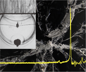
In the first case (figure 15), $\unicode[STIX]{x1D6FE}_{v}=1.4$ and $\unicode[STIX]{x1D6FE}_{b}=0.5$ (i.e. the lower bubble is $2.4R_{m}$ away from the ice plate), the bubbles grow into contact with each other during expansion and coalesce when reaching maximum volumes (frame 3). Subsequently, the coalesced bubble starts to contract from both the upper and lower sides, assuming a double-cone shape (frame 4). The upper side is elongated due to the ice plate (frames 5–7) and, therefore, the lower side moves faster and turns into a re-entrant jet that later pierces through the coalesced bubble and comes out at the top (frames 8 and 9, the jet is shown by the image inserted between frames that are captured with ambient illumination, and the jet speed measured at the jet tip is about $62~\text{m}~\text{s}^{-1}$). The jet impact caused a water hammer shock (see the wave front captured in frame 8). The bubble then continues to shrink in a toroidal form until reaching the minimum volume around frame 11 and emits a series of shock waves from different locations along the torus. The shock waves are strong judging from the degree of darkness of the wave fronts, which is confirmed by the high peak pressure shown in figure 18 that was detected by the transducer located right above the upper bubble. In the subsequent frame 14, two reflection waves can be observed that should be from the water–ice and ice–air interfaces, as discussed before. The ice–air interface reflection wave (the upper one) triggered cavitation at its rear in frame 15, indicating its nature of being an expansion wave. Ice breaking is observed after the shock waves in frames 14 and 15. Fractures initiate from the top of the ice as a result of the tension caused by the expansion wave. The high pressure peak and ice breaking effect should be attributed to the higher energy of the coalesced bubble compared to that of a single bubble. The coalesced bubble manages to collapse to a relatively small volume, reaching a high compression level of its gas contents for more intensive shock wave emissions.

Figure 16. High-speed images of two bubbles vertically positioned below an ice plate. The inter-bubble distance $\unicode[STIX]{x1D6FE}_{b}$ is 1.0. The upper bubble–ice distance $\unicode[STIX]{x1D6FE}_{v}$ remains 1.4. Frame width, 58 mm. The bubbles jet towards each other and turn into toroidal forms before collapsing. The shock waves are unable to cause visible fractures in the ice.

In the second experiment case (figure 16), $\unicode[STIX]{x1D6FE}_{b}$ is increased to 1.0 (i.e. the lower bubble is $3.4R_{m}$ from the ice plate) when $\unicode[STIX]{x1D6FE}_{v}$ is kept at 1.4. The two bubbles expand in almost spherical shapes, flattened on the proximal sides only when reaching the maximum volumes (frames 2). During the following contraction phase, the bubbles hinder each other on the proximal sides and contract faster on the distal sides. The distal side of the lower bubble turns into a jet, which is also shown by the inserted images with ambient illumination that lights up the bubble interior. The jet penetrates the bubble in frame 5 with a speed of about $67~\text{m}~\text{s}^{-1}$, causing a protrusion at the proximal side that grows dramatically in volume in the next few frames. The distal side of the upper bubble is elongated due to the ice plate and then turns into a jet later in frames 6 and 7, and both bubbles become toroidal. The jet reaches a speed of over $190~\text{m}~\text{s}^{-1}$ measured at the jet tip. The high speed is possibly caused by a collision of liquid at the bubble top, as indicated in frame 5. The collision casts liquid downward to form the re-entrant jet. Subsequently, a series of shock waves are emitted successively in frames 8–10. They should be mainly induced by the collapse of the toroidal bubbles and collisions between jets or jet and liquid surrounding the bubbles. In the re-expansion phase, as shown by the last two frames, the growth in the volume of the jet-induced protrusions is obvious. This also indicates that the content of the bubbles has been transported into the protrusions. In this experiment case, the shock waves are unable to crack the ice plate, and it could be attributed to the strong jetting behaviour induced by bubble interaction. More of the bubbles’ energy is distributed to the motion of the jets, and the formation of the jet-induced protrusions reduces the level of compression inside the bubbles. Thus, the shock wave intensity is lessened, which is confirmed by the low pressure peak shown in figure 18, less than one fifth of that of the previous case where the bubble coalesced. Actually, the pressure peak and ice breaking capability of two bubbles with the current $\unicode[STIX]{x1D6FE}_{b}$ is even weaker than that of a single bubble where $\unicode[STIX]{x1D6FE}=1.4$ (see figure 3). This situation is similar to that in figure 6 where the horizontally positioned bubble pair with strong jetting was also unable to crack the ice.

In the third case (figure 17), $\unicode[STIX]{x1D6FE}_{b}$ is increased to 1.5. The bottom of the lower bubble turns into a jet that impacts on the opposite side of the bubble. The impact induces a pressure wave, as captured in frame 5, and a protrusion that grows in the subsequent frames. The lower bubble then becomes toroidal and collapses in frame 6, emitting a series of shock waves. The morphology of the upper bubble is more complicated. Overall, the ice plate and the collapsing lower bubble will impede the contraction at the top and the bottom part of the upper bubble, respectively. In the current case, the two impeding effects are relatively balanced and the contraction from the lateral parts of the upper bubble becomes predominant, leading to splitting of the bubble into two sub-bubbles that collapse and emit two shock waves separately, as in frames 9 and 10. These shock waves are relatively strong as they cause darker wave fronts in the images as well as high pressure peaks, as shown in figure 18. The peaks are of similar magnitude to that of the shock waves from the coalesced bubble with $\unicode[STIX]{x1D6FE}_{b}=0.5$, and also higher than that of a single bubble with $\unicode[STIX]{x1D6FE}=1.4$. This may be attributed to the high compression level of the upper bubble contents when the bubble shrinks to such small volume before emitting shock waves. In addition, before the upper bubble splits, its upper and lower tips both flip inward (frame 9), possibly forming two jets pointing towards each other. This is hard to distinguish but can be inferred as the two sub-bubbles move towards each other after the split, see frames 11 and 12.

Figure 17. High-speed images of two bubbles vertically positioned below an ice plate. The inter-bubble distance $\unicode[STIX]{x1D6FE}_{b}$ is 1.5. The upper bubble–ice distance $\unicode[STIX]{x1D6FE}_{v}$ remains at 1.4. Frame width, 45 mm. The upper bubble splits and the lower bubble jets upwards. Fractures appear in the ice after the shock waves from the upper bubble.

Figure 18. Pressure of the shock waves emitted by the vertically placed collapsing bubble pairs of different inter-bubble distances $\unicode[STIX]{x1D6FE}_{b}$ with a fixed bubble–ice distance $\unicode[STIX]{x1D6FE}_{v}$. Pressure is measured by the transducer at the centre of the wall surface right above the upper bubble.

In the above, three experiment cases are presented with two bubbles vertically placed below an ice plate with a fixed bubble–ice distance $(\unicode[STIX]{x1D6FE}_{v}=1.4)$ and varying inter-bubble distances. The bubble-induced shock wave peak pressure and the ice breaking capability is suppressed when the pair of bubbles is at medium distances $(\unicode[STIX]{x1D6FE}_{b}=1.0)$. In this case, two bubbles can be less effective than a single bubble in ice breaking. In the following, experiment cases with varying bubble–ice distance $\unicode[STIX]{x1D6FE}_{v}$ were carried out to investigate its influences. Four extra cases with $\unicode[STIX]{x1D6FE}_{b}$ being 1.5 and $\unicode[STIX]{x1D6FE}_{v}$ being 0.5, 0.8, 1.1 and 2.0 are shown in figures 19–23. As in these and the previous cases, the lower bubble always has the tendency to move towards the upper bubble and the ice plate. It develops an upward jet that impinges on the opposite side of the bubble and creates a protrusion, if the bubble pair is not coalescing. The water hammer effect of the jet causes pressure waves observed in some of the shadowgraphs (see, for example, frame 4 in figure 20, frame 3 in figure 21 and frame 6 in figure 23). Then the lower bubble collapses in a toroidal form with shock wave emission. The upper bubble, on the other hand, may split as in the previous case $(\unicode[STIX]{x1D6FE}_{v}=1.4)$, or either jet towards the ice plate ($\unicode[STIX]{x1D6FE}_{v}=0.5$, 0.8 and 1.1) or the lower bubble $(\unicode[STIX]{x1D6FE}_{v}=2.0)$ when $\unicode[STIX]{x1D6FE}_{b}=1.5$. The regime of the jetting direction depending on $\unicode[STIX]{x1D6FE}_{v}$ and $\unicode[STIX]{x1D6FE}_{b}$ will be discussed in § 3.5. In the first three cases where $\unicode[STIX]{x1D6FE}_{v}$ is 0.5, 0.8 and 1.1 (figures 19, 20 and 21, respectively), the bottom of the upper bubble first elongates due to the contracting lower bubble, and then quickly retracts and turns into an upward jet that impinges on the ice surface or the opposite bubble wall. As shown by the pressure curves, the jet impact in each case causes a sharp water hammer pressure preceding the pressure wave emitted by the collapse of the bubble (in toroidal form due to jetting). The difference is in the pressure magnitude.

Figure 19. High-speed images of two bubbles vertically positioned below an ice plate. The inter-bubble distance $\unicode[STIX]{x1D6FE}_{b}$ is 1.5. The upper bubble–ice distance $\unicode[STIX]{x1D6FE}_{v}$ is 0.5. Frame width, 45 mm.

Figure 20. High-speed images of two bubbles vertically positioned below an ice plate. The inter-bubble distance $\unicode[STIX]{x1D6FE}_{b}$ is 1.5. The upper bubble–ice distance $\unicode[STIX]{x1D6FE}_{v}$ is 0.8. Frame width, 45 mm.

The experiment with $\unicode[STIX]{x1D6FE}_{v}=0.5$ is shown in figure 19 for shock waves and figure 22(a) for jetting. The upper bubble grows into contact with the ice plate and forms a jet from its bottom that impinges onto the ice surface (frames 9–11, figure 19 and frames 1–5, figure 22a). The jet speed reaches about $100~\text{m}~\text{s}^{-1}$ before impact, and the impingement induced a water hammer pressure shown as the sharp rise on the corresponding pressure curve in figure 24. Such a jet also causes a concentrated ice fracture on the impingement site, as pointed out in frame 11 in figure 19. Subsequently, the bubble collapses onto the ice surface in a toroidal form with a shock wave emitted from the torus, as captured in frames 13 and 14, figure 19. The shock waves are intense with a high pressure peak detected by the transducer on the boundary, which is depicted in figure 24, indicating that the gas in the toroidal bubble could be relatively highly compressed.

Figure 21. High-speed images of two bubbles vertically positioned below an ice plate. The inter-bubble distance $\unicode[STIX]{x1D6FE}_{b}$ is 1.5. The upper bubble–ice distance $\unicode[STIX]{x1D6FE}_{v}$ is 1.1. Frame width, 45 mm. Both the upper bubble and the lower bubble jets upwards. Fractures appear in the ice after the shock waves from the upper bubble.

Figure 22. High-speed images of the upper bubble of the vertically placed collapsing bubble pair with $\unicode[STIX]{x1D6FE}_{b}=1.5$ with ambient illumination to visualize bubble interior and jet. (a) $\unicode[STIX]{x1D6FE}_{v}=0.5$ (b) $\unicode[STIX]{x1D6FE}_{v}=0.8$ and (c) $\unicode[STIX]{x1D6FE}_{v}=1.1$.

For the case when $\unicode[STIX]{x1D6FE}_{v}=0.8$, as shown in figure 20, the upper bubble is not in direct contact with the ice plate at maximum expansion. A gap remains between the bubble and the ice during the bubble contraction phase. The bottom of the bubble turns into a jet that impacts the upper bubble wall and then the ice plate. Details of the jet are depicted in figure 22(b), where a jet speed up to about $170~\text{m}~\text{s}^{-1}$ before impacting on the opposite bubble wall is measured. The impact generates a water hammer shock wave, as captured in frame 9, figure 20, appearing as the dim wave fronts mainly on the lateral side of the gap because the wave propagation in other directions is blocked by the bubble. The pressure of the water hammer shock is also recorded and shown in figure 24. The jet impingement induces a protrusion at the gap (frames 5 and 6, figure 22b). Subsequently, the toroidal bubble shrinks and the protrusion grows rapidly. The growth even continues after the collapse of the toroidal bubble, see frames 7 and 8, figure 22(b). Again it indicates that the bubble contents are being entrained into the protrusion. It would reduce the compression level of the gas in the toroidal bubble before rebounding and emitting shock waves. This may explain the low pressure peaks of the shock waves after the water hammer pressure peak, as depicted in figure 24, especially compared to that of the previous case when $\unicode[STIX]{x1D6FE}_{v}=0.5$ where the bubble behaviour was similar, except for the absence of the jet-induced protrusion.

Figure 23. High-speed images of two bubbles vertically positioned below an ice plate. The inter-bubble distance $\unicode[STIX]{x1D6FE}_{b}$ is 1.5. The upper bubble–ice distance $\unicode[STIX]{x1D6FE}_{v}$ is increased to 2.0. Frame width, 61.0 mm.

Figure 24. Pressure of shock waves induced by the collapsing bubble pairs at different bubble–ice distances $\unicode[STIX]{x1D6FE}_{v}$ with a fixed inter-bubble distance $\unicode[STIX]{x1D6FE}_{b}$.

The case when $\unicode[STIX]{x1D6FE}_{v}=1.1$ is shown in figure 21 and also figure 22(c) for details of the upper bubble jet. The upper bubble manages to shrink to a smaller volume before developing a jet as the effect from the wall is lessened compared to the previous case, see frame 6, figure 21. The jet that forms at the bottom of the upper bubble acquires a speed of approximately $260~\text{m}~\text{s}^{-1}$ and generates a relatively high water hammer pressure upon impingement onto the opposite bubble wall (frame 7, figure 21 or frames 5 and 6, figure 22c). The water hammer pressure reaches two times of that in the previous cases, as reflected in figure 24. Due to the elongated shape at the bottom of the upper bubble, the liquid converges and collides before producing the jet and the collision may be the reason for the high jet speed. Apart from the above, the shock wave from the subsequent bubble collapse also has a relatively high peak pressure, which may be a result of the possible high level of gas compression inside the bubble because it has shrunk to a relatively small volume before rebounding.

Finally, for $\unicode[STIX]{x1D6FE}_{v}=2.0$, as shown in figure 23, the lower bubble jets and collapses toroidally, with the water hammer pressure wave and the collapse shock wave visible in frames 6 and 8, respectively. The upper bubble jets and collapses towards the lower bubble rather than the ice plate and is less retarded in contraction due to the larger bubble–ice distance. Its shock wave emission is captured in frame 10. The outer wave fronts should be due to the jet impact and the inner fronts should be due to the toroidal bubble collapse. The bubble reaches a small volume before emitting shock waves and the wave fronts are relatively dark in the images, both indicating a comparatively high pressure; however, the bubble–ice distance is too large for ice fracturing, and the pressure recorded by the transducer is also relatively low.

In the above experiments, the water hammer pressure induced by the jet impingement on the opposite bubble wall or directly on the ice surface was captured on shadowgraph images or by the pressure transducer. It can also reach a high pressure peak and cause damage of the ice. The damaged ice plate in the three experiment cases with $\unicode[STIX]{x1D6FE}_{v}=0.5$, 0.8 and 1.4 and $\unicode[STIX]{x1D6FE}_{b}$ fixed at 1.5 are shown in figure 25. There is a small area of dense fracture concentrated at the impact site at the centre of the plate, as shown by the photo of ice for $\unicode[STIX]{x1D6FE}_{v}=0.5$, which is likely to be caused by the water hammer effect. This fracture is also shown in the shadowgraph of figure 19, first appearing in frame 11 upon jet impact and then intensified in frames 13 and 14 when the shock waves from the collapse of the toroidal bubble enter the ice plate. On the other hand, the extensive radial crack of the same ice plate should be caused by the toroidal bubble shock waves. For $\unicode[STIX]{x1D6FE}_{v}=1.4$, the ice plate only has radial cracks caused by the shock waves from the upper bubble (figure 17). For $\unicode[STIX]{x1D6FE}_{v}=0.8$, the shock waves are unable to fracture the ice as explained before, but the jet impact resulted in fractures on the impact site which is the only visible damage of the ice plate.

Figure 25. Photograph of ice damaged by vertical bubble pair. (a) Radial fractures caused by the shock wave, central fracture induced by jet impact. $\unicode[STIX]{x1D6FE}_{v}=0.5$, $\unicode[STIX]{x1D6FE}_{b}=1.5$. (b) Radial fractures caused by the shock wave, no jet damage in the centre. $\unicode[STIX]{x1D6FE}_{v}=1.4$, $\unicode[STIX]{x1D6FE}_{b}=1.5$. (c) Central fracture induced by jet impact, no radial fractures induced by the shock wave. Here $\unicode[STIX]{x1D6FE}_{v}=0.8$ and $\unicode[STIX]{x1D6FE}_{b}=1.5$.

In this section, experiments have been presented with two bubbles vertically placed below an ice plate with varying inter-bubble and bubble–ice distances. The ice breaking capability did not vary monotonously with either of the distances. The prominent jetting behaviour at medium bubble distances tends to weaken the collapse and the associated shock wave (for example, the case with $\unicode[STIX]{x1D6FE}_{b}=1.0$, $\unicode[STIX]{x1D6FE}_{v}=1.4$ shown in this section, as well as the cases with $\unicode[STIX]{x1D6FE}_{v}$ over 1.4 as will be shown in § 3.5). In such cases, two bubbles can be less effective than a single bubble in ice breaking. On the other hand, there are also scenarios where ice breaking is enhanced, for example, when the bubbles coalesce, or when the upper bubble manages to shrink to a relatively small volume under the joint effect of the ice plate and the lower bubble and emits stronger shock waves. In addition, under the influence of the lower bubble, the jet of the upper bubble can be more destructive, for example, obtaining a speed up to $260~\text{m}~\text{s}^{-1}$ at $\unicode[STIX]{x1D6FE}_{b}=1.5$ and $\unicode[STIX]{x1D6FE}_{v}=1.1$, and causes severer damage than a single bubble at the same standoff distance. The jet may either fracture the ice directly on the impingement site or cause a strong water hammer shock when impacting on the opposite bubble wall.

Figure 26. High-speed images of two horizontally positioned bubbles collapsing below an ice plate. The inter-bubble distance $\unicode[STIX]{x1D6FE}_{b}$ is 0.88 and the bubble–ice distance $\unicode[STIX]{x1D6FE}_{h}$ is kept as 2.6. Frame height, 14.0 mm. Ambient illumination is used to visualize the interior of the bubbles.

3.4 Bubble characteristics

In the previous sections, high-speed images indicated that deficiency in ice breaking is induced at medium inter-bubble distances, which is assumed to be associated with the relatively strong jetting behaviour of the bubbles. In this section, jet energy and other bubble characteristics will be investigated in order to verify the assumption. Bubble characteristics are measured from experiment cases where the bubble pair is horizontally placed under an ice plate of 20 mm freely floating on a water surface with $\unicode[STIX]{x1D6FE}_{b}$ varying from 0.25 to 2.0, while the bubble–ice distance $\unicode[STIX]{x1D6FE}_{h}$ is fixed at 2.6 whereby the jets are directed towards each other with hardly any inclination. A typical example of jets traversing the bubbles’ interior is given by high-speed images in figure 26, captured using ambient illumination instead of shadowgraphing. The images start with the formation of two jets from the distal sides of the bubbles. The jets are conical with round heads and elongate towards each other. In frames 3 and 4 the jet tips penetrate the proximal sides of the bubbles and cause protrusions (the dark cloud between the bubbles) that collide with each other in the middle of the configuration. The bubbles then become toroidal and later collapse to the minimum volumes in frame 6. In this phase the contents of the bubbles are injected into the protrusions which grow in sizes, as shown in the last three frames. As a result, the volumes of the rebounding toroidal bubbles are small compared to the protrusions. Apart from the above, jet liquid splashes inside the bubbles when the jets impact the proximal bubble surfaces and acts against the collapsing bubble boundary, as shown in frames 4 and 5. All these may weaken the bubble collapse intensity and, hence, reduce the shock wave strength.

In the following analysis the instantaneous kinetic energy of the jet at a certain moment when travelling through the interior of the bubble is estimated as

(3.1)$$\begin{eqnarray}e_{jet}={\textstyle \frac{1}{2}}\unicode[STIX]{x1D70C}Vu_{jet}^{2},\end{eqnarray}$$

where $\unicode[STIX]{x1D70C}$ is the water density, $V$ is the jet volume and $u_{jet}$ is the instantaneous jet speed measured at the jet tip. Here $e_{jet}$ is in dimensional units. The jet volume is calculated deeming the jet as a cone that has different cross-sectional radii along its axis, and the radii are measured from the images. For instance, in figure 27 we take 11 cross-sections on the jet of the left bubble. The cross-sections are marked as A0–B0, A1–B1, …, A10–B10 and the radii of the corresponding cross-sections are denoted by$R_{0},R_{1},\ldots ,R_{10}$, respectively. The section intervals are denoted by $D_{1},D_{2},\ldots ,D_{10}$, respectively. Therefore, we have the left jet’s volume $V_{left}$ at this moment as the summation of volumes of 10 circular truncated cones,

(3.2)$$\begin{eqnarray}V_{left}=\frac{1}{3}\unicode[STIX]{x03C0}\mathop{\sum }_{i=0}^{9}D_{i+1}(R_{i}^{2}+R_{i+1}^{2}+R_{i}R_{i+1})\end{eqnarray}$$

and the jet volume $V$ in (3.1) is the average of the two jets of the two bubbles.

Figure 27. Estimation of volumes of the re-entrant jets that form during the collapse of two interacting bubbles under an ice plate.

Based on the above, bubble characteristics are discussed in the following. First, the process of a jet penetrating through the bubble is investigated. Figure 28 shows the history of jet displacement and energy from jet formation till impact on the opposite bubble walls. The time axis is scaled to the first oscillation period of the bubble, $t_{osc}$. The displacement of the jet tip is denoted as $x_{jet}$ and scaled to $R_{m}$. As shown, when the jets advance inside the bubbles, $x_{jet}$ changes almost linearly with time, which means that the speed measured at the jet tip is nearly constant. In figure 28, $e_{jet}/E_{b}$ reflects the portion of the bubble energy $E_{b}$ distributed to the motion of the jet and is plotted as functions of time scaled to $t_{osc}$. The jet energy increases with time because the jet volume increases as the jet advances inside the bubble, and $e_{jet}/E_{b}$ reaches the maximum right before the jet impacts the opposite bubble wall. For the convenience of comparison between different bubbles, the kinetic jet energy in the following discussions is taken as the value of $e_{jet}$ at the moment right before the jet impacts the bubble wall and is denoted by $E_{jet}$.

Figure 28. Variation of the displacements at the jet tips, $x_{jet}$, scaled to the maximum bubble radius $R_{m}$, with $\unicode[STIX]{x1D6FE}_{b}=0.75$, 0.88, 1.00 and 1.25, and variation of the instantaneous kinetic energies of the jets, $e_{jet}$, scaled to the potential energy of the bubble, $E_{b}$, during the development of the jets inside two bubbles horizontally initiated with $\unicode[STIX]{x1D6FE}_{b}=0.88$ below a 20 mm-thick ice place at $\unicode[STIX]{x1D6FE}_{h}=2.6$. The coordinate origin for the displacement is set as the middle point between the two bubble centres.

Next, the jet speeds under various inter-bubble distances are shown in figure 29. The speed $\overline{u}_{jet}$ here is the average of the jet speeds of the two bubbles. The speed is measured at the jet tips and averaged over the process of the jet traversing through the bubble interior. In general, $\overline{u}_{jet}$ increases with the inter-bubble distance $\unicode[STIX]{x1D6FE}_{b}$. When the two bubbles are initiated closely, the small space between the bubbles does not allow full development of the jets and, thus, the jet speed is lower. As $\unicode[STIX]{x1D6FE}_{b}$ increases, the jet speed increases with a small peak of about $70{-}80~\text{m}~\text{s}^{-1}$ around $\unicode[STIX]{x1D6FE}_{b}=0.6{-}0.7$. For $\unicode[STIX]{x1D6FE}_{b}$ increasing over 1.0, the mutual influence between the bubbles reduces and each bubble reaches a smaller volume and a higher contraction speed before the jets form. Therefore, the jet, which forms after a local acceleration on the contracting bubble surface, continued to grow.

Figure 29. Variation of jet speed $\overline{u}_{jet}$ with the inter-bubble distance, $\unicode[STIX]{x1D6FE}_{b}$. The bubble pair is horizontally placed below a 20 mm-thick ice plate at $\unicode[STIX]{x1D6FE}_{h}=2.6$. The error bars represent a standard deviation of $\overline{u}_{jet}$.

Although the jet speed increases with $\unicode[STIX]{x1D6FE}_{b}$, the maximum volume of the jet decreases as the jet formation is delayed. Thus, the variation of the kinetic jet energy is not monotonous with $\unicode[STIX]{x1D6FE}_{b}$, as plotted in figure 30. At small or large $\unicode[STIX]{x1D6FE}_{b}$, $E_{jet}$ (the jet energy right before penetrating the bubble) is relatively small because of a low jet speed or small jet volume, respectively. Maximum $E_{jet}$ is reached around $\unicode[STIX]{x1D6FE}_{b}=0.6$. At such inter-bubble distance, the jet speed has grown (see figure 29) and the jet volume is still relatively large. Thus, the kinetic energy of the jet is maximized. Figure 30 also shows the result of ice breaking where the hollow marks denote that the 20 mm-thick ice plate is unlikely to be fractured after the bubbles collapse. The incapability to break ice occurs merely within the range of $0.5<\unicode[STIX]{x1D6FE}_{b}<1.25$. This coincides with the range where the jet energy is above 0.045 J or $E_{jet}/E_{b}$ over 0.11, i.e. where more of the bubble energy is distributed to the motion of the jets compared to that in other $\unicode[STIX]{x1D6FE}_{b}$ ranges.

Figure 30. Variation of the kinetic jet energy and the shock wave energy (both scaled to the potential energy of the bubble, $E_{b}$) with the inter-bubble distance $\unicode[STIX]{x1D6FE}_{b}$ at $\unicode[STIX]{x1D6FE}_{h}=2.6$. The hollow triangle denotes that the 20 mm-thick ice plate is not fractured in over 80 % of the experiment cases carried out at the corresponding $\unicode[STIX]{x1D6FE}_{b}$. The error bars represent standard deviation.

The energy of the shock wave induced during the collapse of the bubble pair is denoted as $E_{sw}$, which is estimated from the output of the transducer located at the wall centre as

(3.3)$$\begin{eqnarray}E_{sw}=\frac{4\unicode[STIX]{x03C0}d^{2}}{\unicode[STIX]{x1D70C}c}\int p^{2}(t)\,\text{d}t,\end{eqnarray}$$

where $\unicode[STIX]{x1D70C}$ and $c$ are respectively the density of water and sound speed in water, $p(t)$ is the pressure calculated from the transducer output voltage, as in (2.6), where the reflection due to the wall surface has been excluded, $d$ is the distance from the shock wave emission site to the centre of the transducer’s receiving end (measured from the images). In figure 30 we plot $E_{sw}$ along with the jet energy and scaled to the bubble energy $E_{b}$ estimated by (2.2). The results indicate that the shock waves inherit a large portion of the bubble energy that has coalesced at small inter-bubble distances, but the shock wave energy reduces rapidly to below 15 % of $E_{b}$ as $\unicode[STIX]{x1D6FE}_{b}$ increases to 0.5–1.25. This coincides with the region where the jet energy is found relatively high and where the ice breaking capability is suppressed. This supports the previous assumptions that the bubble pair is unable to fracture the ice because more of the bubble energy that could have been released by shock waves is distributed to the motion of jets. As $\unicode[STIX]{x1D6FE}_{b}$ further increase, the jet energy decreases, the shock wave energy grows and the ice breaking capability increases again.

Figure 31. Variation of the displacement of the bubble centre, $x_{Rmin}$, scaled to the maximum bubble radius, $R_{m}$, and the dimensionless first oscillation period, $\unicode[STIX]{x1D70F}_{osc}$, non-dimensionalized by the Rayleigh collapse time, as functions of the dimensionless inter-bubble distance $\unicode[STIX]{x1D6FE}_{b}$ at $\unicode[STIX]{x1D6FE}_{h}=2.6$. Ice thickness, 20 mm. The error in $x_{Rmin}/R_{m}$ and $\unicode[STIX]{x1D70F}_{osc}$ due to spatial and temporal resolution are 0.013 and 0.02, respectively.

The displacements of the bubble centres and the oscillation periods of the bubbles at various inter-bubble distances with $\unicode[STIX]{x1D6FE}_{h}=2.6$ are shown in figure 31. The centre displacement $x_{Rmin}$ denotes the distance between a bubble’s initial centre and its geometry centre when it collapses to the minimum volume. During the collapse phase, the liquid converging towards the centre of one bubble will pull the other bubble. Thus, the contraction of the proximal side of each bubble is hindered and even stopped, while the contraction of the distal side is enhanced. Therefore, the bubbles appear to be moving towards each other. As indicated, at large inter-bubble distances, the bubble centre displacement is small since the interaction between the bubbles is weak. As the inter-bubble distance decreases, the interaction becomes stronger and the displacement of the bubble centre grows, reaching a maximum at around $\unicode[STIX]{x1D6FE}_{b}=0.9$. As $\unicode[STIX]{x1D6FE}_{b}$ further reduces, the bubbles start to strongly push each other away in the expansion phase before collapsing towards each other in the contraction phase. As a result, $x_{Rmin}$ becomes smaller.

The average dimensionless duration of the first oscillation of the two bubbles is denoted by $\unicode[STIX]{x1D70F}_{osc}$, which is $t_{osc}$ scaled to the Rayleigh collapse time, $9.06\times 10^{-4}~\text{s}$, as estimated in § 2. In figure 31 we plot $\unicode[STIX]{x1D70F}_{osc}$ as a function of $\unicode[STIX]{x1D6FE}_{b}$. Note that $\unicode[STIX]{x1D70F}_{osc}$ gradually decreases as $\unicode[STIX]{x1D6FE}_{b}$ increases, which is also a result of bubble interaction. Since the bubbles are in-phase, each bubble pulls the other one towards its collapsing centre during the contraction phase. Thus, for each bubble, the side proximal to the other bubble will be impeded in contracting and this tends to increase the collapse time of the bubble. On the other hand, the side distal to the other bubble should be accelerated in contracting, which could reduce the collapse time. However, instead of contracting more rapidly, the distal side turns into a re-entrant jet. The jet reaches the other side of the bubble very fast but leaves the distal side contracting much slower. When $\unicode[STIX]{x1D6FE}_{b}$ reduces, such interaction is strengthened. Therefore, the total time for the oscillation of the bubble is prolonged as $\unicode[STIX]{x1D6FE}_{b}$ gets smaller.

Figure 32. Regime diagram of the inter-bubble distance $\unicode[STIX]{x1D6FE}_{b}$ and the bubble–ice distance $\unicode[STIX]{x1D6FE}_{h}$, showing the ice breaking results for a horizontally placed bubble pair.

3.5 Ice breaking results for different $\unicode[STIX]{x1D6FE}_{b}{-}\unicode[STIX]{x1D6FE}_{h}$ regions

In §§ 3.2 and 3.3 both the inter-bubble distance $\unicode[STIX]{x1D6FE}_{b}$ and the bubble–ice distance $\unicode[STIX]{x1D6FE}_{h}$ were demonstrated to influence ice breaking capability of the bubble pair through comparisons by changing each parameter separately. To obtain an overview, the ice breaking results for different combinations of the two parameters ($\unicode[STIX]{x1D6FE}_{b}$ ranging from 0.25 to 2.0 and $\unicode[STIX]{x1D6FE}_{h}$ (or $\unicode[STIX]{x1D6FE}_{v}$) from 0.5 to 2.0) are presented in this section by regime diagrams for the horizontally (figure 32) and vertically (figure 36) positioned bubble pair. In the two regime diagrams, the possibility of ice breaking (the ice plate thickness being 28 mm) is plotted at each point corresponding to a certain combination of $\unicode[STIX]{x1D6FE}_{b}$ and $\unicode[STIX]{x1D6FE}_{h}$ ($\unicode[STIX]{x1D6FE}_{v}$). The possibility is the ratio between the number of experimental cases where visible fracturing is found on high-speed images to the total number of cases carried out at this combination. To help explain the results, the variation of shock wave pressure peak with $\unicode[STIX]{x1D6FE}_{b}$ is also given for each $\unicode[STIX]{x1D6FE}_{h}$ ($\unicode[STIX]{x1D6FE}_{v}$) for both the horizontal and vertical configurations, as shown in figures 33 and 37, respectively.

First, the ice breaking results are shown in figure 32 for the horizontally placed bubble pair. Overall, the capacitance for the two bubbles to fracture the 28 mm thick ice plate varies with both $\unicode[STIX]{x1D6FE}_{b}$ and $\unicode[STIX]{x1D6FE}_{h}$ significantly. For $\unicode[STIX]{x1D6FE}_{b}\geqslant 0.5$, the medium bubble–ice distance $\unicode[STIX]{x1D6FE}_{h}=1.1$ appears to be the most suitable for ice breaking among the distances investigated. For other bubble–ice distances, there are ranges of $\unicode[STIX]{x1D6FE}_{b}$ in which the bubble pair is inefficient to cause fracturing of the ice plate. For the closest distance, $\unicode[STIX]{x1D6FE}_{h}=0.5$, the range of weak ice breaking is around $\unicode[STIX]{x1D6FE}_{b}=1.0{-}1.5$. Here the jet moves along the ice surface with strong splashing and pushes the bubble to collapse in a distorted half-torus shape with comparatively less intensive shock wave emission. The shock waves are unable to fracture the ice even at such a close bubble–ice distance, as demonstrated and discussed in § 3.2. For $\unicode[STIX]{x1D6FE}_{h}=0.8$, there are two less-effective ice breaking regions according to the regime diagram and the variation trend of the peak pressure plotted against $\unicode[STIX]{x1D6FE}_{b}$ in figure 33. The first is when $\unicode[STIX]{x1D6FE}_{b}$ is around 1.0. A representative series of high-speed images of the bubble is shown in figure 34(a). At this distance, shock waves emit from multiple locations along the bubbles, as captured in frames 3 and 4. The emission being scattered may be the reason for the peak pressure of the shock waves being lower compared to that in the case with $\unicode[STIX]{x1D6FE}_{b}$ being 1.25, where the shock waves mainly emit from the upper distal sides (see figure 11) of the bubbles. The second is when $\unicode[STIX]{x1D6FE}_{b}$ is larger than 1.5. In this range the bubble shape gradually transforms to that of a single bubble at $\unicode[STIX]{x1D6FE}=0.8$ that is unable to fracture the ice due to issues associated with the jet and the protrusion, as discussed in § 3.1.

Figure 33. Variation of shock wave peak pressure values with inter-bubble distance $\unicode[STIX]{x1D6FE}_{b}$ under different bubble–ice distances $\unicode[STIX]{x1D6FE}_{h}$ for a horizontally placed bubble pair.

For further distances of $\unicode[STIX]{x1D6FE}_{h}=1.1{-}1.7$, the ice breaking effect is stronger with $\unicode[STIX]{x1D6FE}_{b}$ around 0.5 due to bubble coalesce, as discussed in § 3.2. But interestingly, when the two bubbles are initiated at an even closer distance $(\unicode[STIX]{x1D6FE}_{b}=0.25)$, the peak pressure and ice breaking possibility both reduce. High-speed images of bubble morphology of a typical example in this region is shown in figure 35 using both shadowgraph (a) and ambient illumination (b). After the two bubbles coalesced in frames 1 and 2 in figure 35(a), the liquid at the two lower distal sides of the bubbles moves in opposite directions along with the contracting bubble boundary and collides in frame 5. The collision leads to liquid splashing inside the merged bubble which is shown in frame 3 onwards in figure 35(b). The splashing liquid soon floods the interior of the bubble and impacts with the contracting bubble surface, see frames 4–6 of figure 35(b). The splashing could be a strong interference against the subsequent collapse of the merged bubble. Therefore, it may have an adverse effect on the compression of the bubble’s gas contents and subsequent shock wave emission, and, thus, resulted in the reduced peak pressure and ice breaking capability at $\unicode[STIX]{x1D6FE}_{b}=0.25$. Such liquid splashing becomes less intense when the bubble–ice distance increases.

Figure 34. (a) High-speed images of a bubble collapsing at $\unicode[STIX]{x1D6FE}_{b}=1.0$ and $\unicode[STIX]{x1D6FE}_{h}=0.8$ and (b) shock wave pressure for the same experiment scenario. Shock waves are emitted from different places along the toroidal bubble and the pressure peaks are relatively low compared to other cases, for example, that with $\unicode[STIX]{x1D6FE}_{b}=1.25$ and $\unicode[STIX]{x1D6FE}_{h}=0.8$. (c) Shock wave pressure for $\unicode[STIX]{x1D6FE}_{b}=0.25$ and $\unicode[STIX]{x1D6FE}_{h}=1.4$, where the bubbles coalesced at close proximity.

Figure 35. (a) Shadowgraph images of two bubbles coalescing and collapsing at $\unicode[STIX]{x1D6FE}_{b}=0.25$ and $\unicode[STIX]{x1D6FE}_{h}=1.4$. (b) The late contraction stage of the bubbles for the same scenario with ambient illumination.

Figure 36. Regime diagram of the inter-bubble distance $\unicode[STIX]{x1D6FE}_{b}$ and the bubble–ice distance $\unicode[STIX]{x1D6FE}_{v}$, showing the ice breaking results for a vertically placed bubble pair. The markers with a magenta rimming denote the case where the upper bubble splits.

Figure 37. Variation of the peak of the shock wave pressure with inter-bubble distance $\unicode[STIX]{x1D6FE}_{b}$ under different bubble–ice distances $\unicode[STIX]{x1D6FE}_{v}$ for a vertically placed bubble pair.

Apart from $\unicode[STIX]{x1D6FE}_{b}=0.25$, the pressure peak variation with $\unicode[STIX]{x1D6FE}_{b}$ is quite similar for $\unicode[STIX]{x1D6FE}_{h}=1.1{-}2.0$, reaching a maximum around $\unicode[STIX]{x1D6FE}_{b}=0.5$ then a minimum around $\unicode[STIX]{x1D6FE}_{b}=1.0$ and increasing again with larger $\unicode[STIX]{x1D6FE}_{b}$. As discussed in §§ 3.1 and 3.2 and also indicated in § 3.4, the jetting behaviour is strong in the range around $\unicode[STIX]{x1D6FE}_{b}=1.0$ and large protrusions are formed, both of which can have an adverse effect on shock wave strength. Nevertheless, for $\unicode[STIX]{x1D6FE}_{h}=1.1$, the shock pressure overall has a higher magnitude as the distance to the transducer is smaller. The ice breaking result in figure 32 is generally in correspondence with the pressure peak variation. In addition, for $\unicode[STIX]{x1D6FE}_{h}=1.7{-}2.0$, the pressure peak is relatively low for $\unicode[STIX]{x1D6FE}_{b}$ over 1.5 or 1.75 when compared to $\unicode[STIX]{x1D6FE}_{h}<1.7$, but the ice still cracked. The ice breaking here may be attributed to an overlapping of the shock waves from the two bubbles (or their reflections from the ice–air interface) somewhere in the ice plate near the centre of the configuration, which cannot be captured by the transducer that is located above one of the two bubbles.

Next, the ice breaking region for the vertically placed bubble pair is shown in figure 36. The results are also depicted by different markers denoting a different possibility of ice fracturing based on the experimental results. The ice breaking trend is closely related to $\unicode[STIX]{x1D6FE}_{b}$ and $\unicode[STIX]{x1D6FE}_{v}$, and similar to the horizontal configuration, $\unicode[STIX]{x1D6FE}_{b}$ being around 1.0 should be avoided for more efficient ice breaking. This is due to the relatively strong jetting behaviour at this inter-bubble distance that brings an adverse effect on shock strength, as discussed earlier. Apart from this, the ice breaking trend here has obvious differences from that of the horizontal bubble pair. It is easiest to fracture the ice plate when placing the upper bubble at a close distance, $\unicode[STIX]{x1D6FE}_{v}=0.5$, or at a medium distance, $\unicode[STIX]{x1D6FE}_{v}=1.1$, to the ice plate, among all the bubble–ice distances investigated. At $\unicode[STIX]{x1D6FE}_{v}=0.5$, the jet of the upper bubble may directly impact the ice plate and has a chance to cause fracturing at the impingement site. In addition, the shock emission is in close proximity to the ice surface, thus, the ice is highly likely to fracture at $\unicode[STIX]{x1D6FE}_{v}=0.5$ regardless of $\unicode[STIX]{x1D6FE}_{b}$. When $\unicode[STIX]{x1D6FE}_{v}$ is increased to 0.8, the ice breaking trend is different. For $\unicode[STIX]{x1D6FE}_{b}<1.0$, the bubbles coalesce and end in a stronger collapse with a higher ice breaking possibility. For $\unicode[STIX]{x1D6FE}_{b}>1.0$, the upper bubble jet produces a protrusion between the bubble and the ice. The strong jetting may reduce the portion of bubble energy that is distributed to shock waves and the protrusion growth may reduce the gas compression level of the toroidal bubble, thus, the bubble emits weaker shock waves, as discussed in § 3.3. As $\unicode[STIX]{x1D6FE}_{b}$ further increases, the upper bubble behaviour becomes similar to that of a single bubble at $\unicode[STIX]{x1D6FE}=0.8$, which is also unable to crack the ice plate due to similar reasons, while the shock waves of the lower bubble are emitted too far to induce ice breaking. Note that in figure 37 the peak pressure for $\unicode[STIX]{x1D6FE}_{b}$ from 1.0 to 1.75 when $\unicode[STIX]{x1D6FE}_{h}=0.8$ is mostly induced by the water hammer pressure when the jet impinges on the transducer and is therefore higher than the pressure peak of the shock waves that are emitted later by the toroidally collapsing bubble, especially at $\unicode[STIX]{x1D6FE}_{b}$ around 1.2–1.5 where the water hammer impingement alone may cause ice damage close to the impact site, but without further fracturing the ice plate since the subsequent shock waves are relatively weak, as illustrated in § 3.3. Such a scenario was not considered a successful ice breaking.

When $\unicode[STIX]{x1D6FE}_{v}$ is increased to 1.1, the peak value of the shock wave pressure at different $\unicode[STIX]{x1D6FE}_{b}$ is in general higher than other $\unicode[STIX]{x1D6FE}_{v}$ and associated with higher ice breaking capability. The only weak spot is at $\unicode[STIX]{x1D6FE}_{b}=1.0$, where the pressure peak is largely reduced. The bubble behaviour in this case is demonstrated in figure 38(a), which shows that the lower half of the upper bubble splits away from the upper part (frame 2 onwards) and collides with the lower bubble. The remaining part collapses towards the ice plate (frames 4 and 5), but neither the water hammer pressure wave or the collapse shock waves of this part are strong enough to cause breaking of the ice plate given that the contents of the upper bubble (and, hence, the energy) has been largely reduced after the split. On the other hand, the lower bubble develops an upward jet and turns toroidal, with a jet-induced protrusion at its top (frame 1). As discussed before, the protrusion reduces the collapse intensity of the toroidal part and as a result, shock wave emissions from the toroidal bubble are too weak to be visualized. The jet along with the protrusion collides with the lower half of the upper bubble, leading to several shock wave emissions in frames 5–7, which are also not strong enough to cause ice breaking.

For $\unicode[STIX]{x1D6FE}_{v}\geqslant 1.4$, the ice breaking trend becomes similar to that for the horizontally placed bubble pair because the bubble–ice interaction plays a less important role in affecting bubble behaviour. The variation trend of the pressure peaks with $\unicode[STIX]{x1D6FE}_{b}$ for $\unicode[STIX]{x1D6FE}_{v}=1.4{-}2.0$ are similar, reaching a minimum while $\unicode[STIX]{x1D6FE}_{b}$ is around 1.0. In this region, the strong counter-jetting of the two bubbles may have affected the collapse strength in several ways, including taking up more bubble energy, and causing protrusions that reduce the compression level of the toroidal bubble, etc., as discussed in §§ 3.3 and 3.4. When $\unicode[STIX]{x1D6FE}_{b}$ exceeds 1.25 for $\unicode[STIX]{x1D6FE}_{v}=1.4{-}2.0$, the pressure peak and ice breaking effect ought to become more similar to that of a single bubble with $\unicode[STIX]{x1D6FE}=\unicode[STIX]{x1D6FE}_{v}$, because on the one hand, the behaviour of the upper bubble becomes closer to that of the single bubble due to the relatively weak bubble interaction, on the other hand, the lower bubble is too far away to cause ice breaking. However, exceptions are observed. For example, in the case when $\unicode[STIX]{x1D6FE}_{b}=1.5$, $\unicode[STIX]{x1D6FE}_{v}=1.4$, which has been discussed in § 3.3, the upper bubble can reach a very small volume before jetting due to the balanced effect from the ice plate and the lower bubble, and, therefore, reaches a higher level of compression inside the bubble and emits stronger shock waves with a peak value higher than that of a single bubble at $\unicode[STIX]{x1D6FE}=1.4$.

As mentioned earlier, the collapse direction of the upper bubble is determined by the effects from both the ice plate and the lower bubble. When the effects are unbalanced, the bubble collapses and jets towards either the ice plate or the lower bubble, otherwise, the bubble would split. The splitting cases are marked out in the regime diagram with magenta boxes in figure 36, which assemble into a ‘splitting zone’. In this zone, if $\unicode[STIX]{x1D6FE}_{v}\leqslant 1.1$, the upper bubble splits into two parts that collapse towards opposite directions. The lower part may jet towards or merge with the lower bubble depending on $\unicode[STIX]{x1D6FE}_{b}$. If $\unicode[STIX]{x1D6FE}_{v}\geqslant 1.4$, the upper bubble manages to shrink to a relatively small volume before splitting or jetting. This means high compression of the bubble contents and may lead to stronger shock waves as reflected by the pressure data in § 3.3.

Figure 38. (a) High-speed images of bubble collapsing at $\unicode[STIX]{x1D6FE}_{b}=1.0$ and $\unicode[STIX]{x1D6FE}_{v}=1.1$, (b) pressure of shock waves induced by a vertical bubble pair of the same scenario.

In this section the ice breaking results are summarized over the $\unicode[STIX]{x1D6FE}_{b}{-}\unicode[STIX]{x1D6FE}_{h}$ ($\unicode[STIX]{x1D6FE}_{v}$) space. The ice breaking capability variation is complex with different inter-bubble and bubble–ice distances. It is related to the shock wave pressure peak induced by the bubble pair, which is closely linked to the bubble morphology, jet characteristics and shock wave emission pattern. The quantitative data suggests that the threshold of the incident pressure peak for the 28 mm-thick ice plate used in the current experiment to break is around 7.5–10 MPa. All cases considered, the most effective ice breaking scenarios for a horizontally placed bubble pair are found when $\unicode[STIX]{x1D6FE}_{h}=1.1$, and the most effective scenarios for the vertically placed pair are found when $\unicode[STIX]{x1D6FE}_{v}=0.5$. Besides, medium inter-bubble distances around $\unicode[STIX]{x1D6FE}_{b}=1.0$ should be avoided to enhance shock wave strength and ice breaking capability for both horizontal and vertical configurations.