


1 Introduction
Surfaces covered by arrayed, filamentous layers anchored to a substrate and exposed to viscous flows are commonly found in nature, and increasingly seen in bio-inspired technology (Mars, Mathew & Ho Reference Mars, Mathew and Ho1999; Wilcock et al. Reference Wilcock, Champion, Nagels and Croker1999; Ghisalberti & Nepf Reference Ghisalberti and Nepf2002; Luhar, Rominger & Nepf Reference Luhar, Rominger and Nepf2008). Living organisms use surfaces with complex textures and their interaction with surrounding fluid flows for a number of tasks: decrease skin friction drag (e.g. seal fur, see Itoh et al. (Reference Itoh, Iguchi, Yokota, Akino, Hino and Kubo2006)), control of flight aerodynamics (e.g. birds’ feathers, see Brücker & Weidner (Reference Brücker and Weidner2014)), increase nutrient and light uptake (e.g. vegetative canopies, see Finnigan (Reference Finnigan2000)), form-drag control via reconfiguration (e.g. tree foliage, see Leclercq & de Langre (Reference Leclercq and de Langre2016)). Ciliated walls and flagella are also commonly found in living organs participating in a number of physiological processes like locomotion, digestion, circulation, respiration and reproduction (see any cellular biology textbook, e.g. Lodish, Berk & Kaiser (Reference Lodish, Berk and Kaiser2007)).
All the mentioned examples clearly show that the geometrical configuration and the mechanical properties of the various filamentous surfaces found in nature conform to the task that needs to be tackled. Thus, the number of free parameters that define a specific type of ciliated layer, or of a specific canopy, is quite large (e.g. density ratios, flexibility, aspect ratios, sizes, levels of submersion, active or passive motions, …) and to incorporate all of them in a comprehensive parametric investigation is an almost impossible task. Here, as in many other previous research efforts, we will focus only on a reduced set of canopy flows where the solidity of the layer is the only feature that differentiates every single realisation. This choice aligns with recent investigations on aquatic plants carried out by Nepf (Reference Nepf2012) and collaborators that used a classification of canopy flows based on only two geometrical properties. The first one is the ratio between the flow depth  $H$ and the canopy height
  $h$ (i.e. the level of submersion, see figure 1), to classify canopies as emergent (
 $H/h=1$), shallow submerged (
 $1<H/h<5$) and deeply submerged (
 $H/h>10$). This definition allows us to classify canopy flows according to the relative importance of the turbulent stresses and the flow-driving pressure gradient (Nepf & Vivoni Reference Nepf and Vivoni2000).

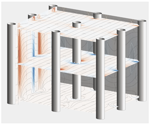
Figure 1. Geometrical parameters governing canopy flows according to Nepf (Reference Nepf2012). In our simulation, the filaments are randomly distributed on the canopy bed, each one occupying an average area  $\unicode[STIX]{x0394}S^{2}$.
In emergent canopies, the turbulence length scale is imposed either by the stem diameter  $d$ or by the average spacing between filaments
  $\unicode[STIX]{x0394}S$ when the latter is smaller than the former (Nepf Reference Nepf2012). The momentum equation for emergent canopy flows reduces to a balance between the drag force and the driving pressure gradient, leading to a self-similar velocity profile which only depends on the ratio
  $a(y)$ of the frontal area
  $dh$ and the canopy volume of influence
  $\unicode[STIX]{x0394}S^{2}h$ (Lightbody & Nepf Reference Lightbody and Nepf2006), i.e.
  $a(y)=d(y)/\unicode[STIX]{x0394}S^{2}$.
Submerged canopies substantially differ from the emergent ones as they feature different regimes whose individual genesis depends on a large number of parameters. A key one is the canopy solidity, defined as the ratio of the frontal area of the canopy and the bed area,
 $$\begin{eqnarray}\unicode[STIX]{x1D706}=\int _{0}^{h}a(y)\,\text{d}y.\end{eqnarray}$$
 It is known that, for extreme values of  $\unicode[STIX]{x1D706}$, the flow reaches two asymptotic regimes (Poggi et al. Reference Poggi, Porporato, Ridolfi, Albertson and Katul2004; Nepf Reference Nepf2012). If
  $\unicode[STIX]{x1D706}$ is much smaller than a threshold value (i.e.
  $\unicode[STIX]{x1D706}\ll 0.1$) then the flow velocity within and above the canopy shows a behaviour comparable to the one observed in a turbulent boundary layer over a rough wall with a dominance of bed drag over canopy form drag (a condition termed sparse regime). Conversely, for large values of
  $\unicode[STIX]{x1D706}$ (i.e.
  $\unicode[STIX]{x1D706}\gg 0.1$), the drag produced by the bed becomes negligible when compared to the canopy one. In this situation, termed dense regime, the drag discontinuity at the tip of the canopy induces the appearance of an inflection point in the mean velocity profile at the canopy edge. Another, often overlooked, inflection may form closer to the bed, where the boundary layer at the wall merges with the mean profile that develops in the core of the canopy.
In a dense regime, these two inflection points divide the intra-canopy flow into separate regions: an inner region, very close to the bed, an outer region, mostly located outside the canopy, and a central region sandwiched between the two. Within this mid-portion of the canopy, it can be assumed that a peculiar Couette flow takes place with a large portion of the short-wavelength fluctuations produced by the meandering of the flow in between the canopy elements. This conceptual, three-layer structure of dense canopy flows was first proposed by Belcher, Jerram & Hunt (Reference Belcher, Jerram and Hunt2003).
Poggi et al. (Reference Poggi, Porporato, Ridolfi, Albertson and Katul2004) carried out an experimental campaign on rigid canopy flows in which they varied the canopy density (the number of stems per unit bed surface, i.e.  $\unicode[STIX]{x0394}S^{2}$). They were able to show that the mean velocity profile does not present a clear inflection point at the canopy edge for values of
  $\unicode[STIX]{x1D706}<0.04$ (i.e. within the sparse regime). Conversely, when
  $\unicode[STIX]{x1D706}>0.1$, the mean velocity profile clearly featured a pronounced inflection point at the tip of the canopy layer in agreement with the observations of Nepf (Reference Nepf2012). Poggi et al. (Reference Poggi, Porporato, Ridolfi, Albertson and Katul2004) also proposed a phenomenological classification for canopy flows: in the sparse regime, the flow is assumed to behave like a boundary layer over a rough wall, while in the dense regimes, the flow can be modelled using a weighted superposition of three distinct zonal flow behaviours determined by the size of the largest eddy that can be locally accommodated. Following the spirit of classical Prandtl’s mixing-layer models, each zone was assumed to set a different length scale. Specifically, in the canopy inner region, i.e.
  $y/h\ll 1$, the flow field is assumed to be characterised by vortices shed by the canopy elements whose size and intensity depend on the diameter of the stems. Supported by the observations of other authors (Raupach, Finnigan & Brunei Reference Raupach, Finnigan and Brunei1996; Finnigan Reference Finnigan2000), the outer region, i.e.
  $y/h\gg 2$, is postulated to behave like a classical boundary layer over a rough wall. Finally, within the region overlapping the innermost and outermost zones, the flow is assumed to be dominated by a mixing layer of constant thickness.
The formation of a mixing-layer flow by the canopy edge is induced by the inflected mean velocity profile that triggers a Kelvin–Helmholtz (KH)-like instability. The latter eventually leads to large scale spanwise vorticity rollers. The size of these structures is comparable to the height of the canopy for unsaturated regimes: i.e. whenever the thickness of the filamentous layer is short enough for the outer flow to be conditioned by the presence of the impermeable, bottom wall (coarse to marginally dense regimes). This system of spanwise vortices, that is believed to govern the bulk of the momentum transport between the outer and the inner regions in dense canopies (Nepf Reference Nepf2012), has also been reported by other authors in other contexts (for example, in turbulent wall flows over porous media, see Jiménez et al. (Reference Jiménez, Uhlmann, Pinelli and Kawahara2001)). Raupach et al. (Reference Raupach, Finnigan and Brunei1996) observed that within the developed mixing layer near the canopy tip, the most unstable streamwise wavelength of the KH instability,  $\unicode[STIX]{x1D6EC}_{x}$, is spatially preserved. Moreover, they also suggested that the ratio of
  $\unicode[STIX]{x1D6EC}_{x}$ and the mixing-layer vorticity thickness
  $\unicode[STIX]{x1D6FF}_{\unicode[STIX]{x1D714}}=\unicode[STIX]{x0394}U/(\unicode[STIX]{x2202}U/\unicode[STIX]{x2202}y)_{max}$ falls within the range,
  $3.5<\unicode[STIX]{x1D6EC}_{x}/\unicode[STIX]{x1D6FF}_{\unicode[STIX]{x1D714}}<5$ (Finnigan Reference Finnigan2000). The same authors (Raupach et al. Reference Raupach, Finnigan and Brunei1996) also showed that, for dense canopies, the ratio between the KH most unstable wavelength and a measure of the vorticity thickness
  $L_{s}=U(h)/\unicode[STIX]{x2202}_{y}U(h)$, obtained by considering the velocity gradient at the canopy tip only, is found to be within the range
  $7<\unicode[STIX]{x1D6EC}_{x}/L_{s}<10$. Indeed, several experiments have confirmed this bound and have put forward an even more stringent relation given by
  $\unicode[STIX]{x1D6EC}_{x}\simeq 8.1L_{s}$. Another three-layer model for dense submerged canopies, similar to the one put forward by Poggi et al. (Reference Poggi, Porporato, Ridolfi, Albertson and Katul2004), has been proposed by Nezu & Sanjou (Reference Nezu and Sanjou2008). They conjectured that the flow behaviour within each layer develops as a consequence of a single dominant generation mechanism enhancing the observed local features while inhibiting the coexistence of other vorticity structures pertaining to neighbouring layers.
The bibliographic survey that has been presented above is just a limited sample of the large body of literature addressing submerged canopies. The main research tool behind the majority of these studies is of experimental nature, thus limited by the presence of the filamentous canopy that renders the use of localised measurements difficult (e.g. laser Doppler velocimetry or particle image velocimetry). Despite these limitations, the literature presents an increasing proliferation of canopy-flow models that need verification and validation through techniques that can provide more detailed insight into the flow fields arising in canopy flows. In particular, the determination of a proper scaling and of robust criteria able to deliver an a priori prediction on the insurgence of particular canopy-flow regimes are still open topics and available analysis and predictions only cover specific situations. Moreover, the condition for the emergence of different intra-canopy flows at intermediate flow regimes and their detailed characterisation are still not well documented, let alone the understanding of the interplay between physical mechanisms as the flow transitions from one regime to another. This lack of understanding is particularly evident in the transitional regime scenario where the main features of the coarse and dense regimes combine in a non-trivial way. As will be shown in the results section, this regime establishes when the positions of the virtual wall seen by the outer flow and the innermost mean velocity inflection point cross. In physical terms, the transition between the two asymptotic regimes corresponds to the formation of a central region in the canopy where the outer flow overlaps with the portion of the flow developing in the region close to the bottom wall. Other potentially relevant mechanisms that have not been considered in depth concern the role of KH-generated spanwise vorticity rollers, their modification by the outer flow structures and their role in redistributing the local momentum within and outside the canopy (Monti, Omidyeganeh & Pinelli Reference Monti, Omidyeganeh and Pinelli2019).
Without pretending to offer a final say on general canopy flows and only by varying the frontal solidity of the canopy  $\unicode[STIX]{x1D706}$, the research presented in this work addresses some of the mentioned research topics where no reliable or validated understanding is available. In particular, through the analysis of the flows arising when changing the canopy solidity
  $\unicode[STIX]{x1D706}$, we will identify the dominant scales of motions that are either enhanced or weakened in different regimes. This understanding allows us to establish a robust macroscopic criterion able to predict the dominant features of canopy flows when
  $\unicode[STIX]{x1D706}$ is varied. The latter is based on the relative positions of the inflection points of the mean velocity profile and the virtual origin seen by the outer flow.
The approach that we have considered to tackle those questions relies on the analysis of a set of highly resolved simulations of a turbulent flow in an open channel bounded by rigid canopies of various solidities, assembled with vertically mounted filaments. The value of  $\unicode[STIX]{x1D706}$ is set within a range of values that generate canopy flows nominally varying from sparse to dense regimes. In particular, we report results obtained using a formulation that directly resolves the intra-canopy flow stem by stem by imposing a zero-velocity condition on each element of the filamentous layer. The manuscript is organised as follows. Section 2 describes the numerical method used to undertake the simulations. Section 3 describes the obtained results. Their analysis is mainly carried out by comparing the statistical and instantaneous characterisations of the canopy-flow fields realised with four different values of the solidity
  $\unicode[STIX]{x1D706}$. Finally, § 4 outlines the most important conclusions with emphasis on the new findings that mainly concern the introduction of a generalised scaling approach for the mean flow statistical values, a novel criterion to predict the canopy-flow regime and new observations on the flow structure of the close-to-the-bed intra-canopy region which is strongly influenced by the internal mean velocity inflection point.
2 The numerical technique
We have simulated the turbulent flows over rigid canopies using an incompressible Navier–Stokes solver developed in house (SUSA, Omidyeganeh & Piomelli Reference Omidyeganeh and Piomelli2013a). In particular, we adopted a large-eddy simulation (LES) formulation where the governing equations are obtained from the full Navier–Stokes equations by filtering out the velocity and pressure fluctuations taking place on all length scales smaller than a spatial filter which width falls within the inertial range of turbulence. In a Cartesian frame of reference, indicating with  $x_{1}$,
  $x_{2}$ and
  $x_{3}$ (i.e.
  $x$,
$x$,  $y$ and
  $z$) the streamwise, wall-normal and spanwise directions and with
  $u_{1}$,
  $u_{2}$ and
  $u_{3}$ the corresponding velocity components (i.e.
  $u$,
$u$,  $v$ and
  $w$), the dimensionless incompressible LES equations for the resolved fields
  $\overline{u}$ and
  $\overline{p}$ read as
 $$\begin{eqnarray}\frac{\unicode[STIX]{x2202}\overline{u}_{i}}{\unicode[STIX]{x2202}t}+\overline{u}_{j}\frac{\unicode[STIX]{x2202}\overline{u}_{i}}{\unicode[STIX]{x2202}x_{j}}=-\frac{\unicode[STIX]{x2202}\overline{P}}{\unicode[STIX]{x2202}x_{i}}+\frac{1}{Re_{b}}\frac{\unicode[STIX]{x2202}^{2}\overline{u}_{i}}{\unicode[STIX]{x2202}x_{j}\unicode[STIX]{x2202}x_{j}}+\frac{\unicode[STIX]{x2202}\unicode[STIX]{x1D70F}_{ij}}{\unicode[STIX]{x2202}x_{j}}+f_{i},\quad \frac{\unicode[STIX]{x2202}\overline{u}_{i}}{\unicode[STIX]{x2202}x_{i}}=0.\end{eqnarray}$$
 In (2.1),  $Re_{b}=U_{b}H/\unicode[STIX]{x1D708}$ is the Reynolds number based on the bulk velocity
  $U_{b}$, the open-channel height
  $H$ and
  $\unicode[STIX]{x1D708}$ is the kinematic viscosity;
  $\unicode[STIX]{x1D70F}_{ij}=\overline{u_{i}u_{j}}-\overline{u}_{i}\overline{u}_{j}$ is the subgrid Reynolds stress tensor (Leonard Reference Leonard1975) that was modelled using the integral length scale approximation approach recently proposed by Piomelli, Rouhi & Geurts (Reference Piomelli, Rouhi and Geurts2015) (see also Rouhi, Piomelli & Geurts (Reference Rouhi, Piomelli and Geurts2016)). The incompressible LES equations (2.1) are space discretised using a second-order accurate, cell centred finite volume method. Pressure and velocity are co-located at the centres of the cells and the approach of Rhie & Chow (Reference Rhie and Chow1983) is used to avoid pressure oscillations. The equations are advanced in time using a second-order, semi-implicit fractional-step procedure (Kim & Moin Reference Kim and Moin1985). In particular, the implicit Crank–Nicolson scheme is implemented for the wall-normal diffusive terms while an explicit Adams–Bashforth scheme is applied to all other terms. The Poisson pressure equation, that needs to be solved at each time step to enforce the solenoidal condition of the velocity field, is transformed into a series of two-dimensional (2-D) Helmholtz equations in the wavenumber space using a fast Fourier transform along the spanwise direction. Each of the resultant elliptic 2-D problems is then solved using a preconditioned Krylov method. In particular, we found the iterative biconjugate gradient stabilised method with an algebraic multigrid preconditioner (boomerAMG, see Henson & Yang Reference Henson and Yang2002) to behave quite efficiently. The code is parallelised using the domain decomposition technique implemented via the MPI message passing library. Further details on the code, its parallelisation and the extensive validation campaign, that have been carried out in other flow configurations, can be found in previous publications (Omidyeganeh & Piomelli Reference Omidyeganeh and Piomelli2011, Reference Omidyeganeh and Piomelli2013a,Reference Omidyeganeh and Piomellib; Rosti, Omidyeganeh & Pinelli Reference Rosti, Omidyeganeh and Pinelli2016).
Unlike other approaches (e.g. Bailey & Stoll Reference Bailey and Stoll2016), our formulation can be considered as a coarse direct numerical simulation in the outer portion of the flow that progressively becomes highly resolved as the canopy is approached. In the outer flow region, the subgrid stress contribution plays only the role of a very mild and stabilising numerical dissipation. Indeed, the ratio between the total and the subgrid energies averaged in time and in the two homogeneous directions, shown in figure 3(a) along the channel height, is always below  $10^{-5}$ for all the canopy configurations. A further indication that the LES filter operates at the end of the turbulence cascade is provided in figure 3(b), showing that the ratio between the time and space averaged eddy viscosity and the physical one is always of order unity or less throughout the whole channel for all the considered stems distributions. In the intra-canopy region, we resolve the canopy stems one by one without the introduction of any model. In particular, the stems embedded in the canopy are represented as rigid, solid, slender cylindrical rods of finite cross-sectional area perpendicularly mounted onto the impermeable bottom wall. To enforce the boundary conditions that each rigid cylinder imposes on the fluid (i.e. zero velocity at the surface of each stem) we used an immersed boundary method (IBM). The latter deals with the presence of the rods, whose locations do not conform with the actual fluid grid, by using a set of nodes distributed along the length of each canopy element (termed Lagrangian nodes). More specifically, the employed IBM associates with each Lagrangian node a set of distributed body forces defined on a compact support centred on each node. At each time step, the intensity of those forces is determined by enforcing a Dirichlet condition, i.e. zero velocity of the fluid, on all the nodes used to discretise each element of the canopy. The size of the support is related to the local grid size and also defines the hydrodynamic thickness of the filament that in our case can be estimated to be
  $2.2\unicode[STIX]{x0394}x$ (Monti et al. Reference Monti, Omidyeganeh and Pinelli2019), or
  $2.2\unicode[STIX]{x0394}z$, since the mesh spacing is the same in the
  $x$ and
  $z$ directions. The adopted IBM and its properties are described and discussed in Pinelli et al. (Reference Pinelli, Naqavi, Piomelli and Favier2010) and Favier, Revell & Pinelli (Reference Favier, Revell and Pinelli2014). The assessment of the IBM, including the calibration of the support of each Lagrangian node required to deliver a resolution comparable to an interface resolved immersed boundary formulation (Fadlun et al. Reference Fadlun, Verzicco, Orlandi and Mohd-Yusof2000) can be found in Monti et al. (Reference Monti, Omidyeganeh and Pinelli2019). In particular, in the given reference we show that, although the details of the boundary layers forming on each stem cannot be properly captured, the wake structure and the drag on each stem are very well predicted. To distribute the stems on the bottom wall, we have subdivided the latter into a Cartesian lattice of uniform squares of area
  $\unicode[STIX]{x0394}S^{2}$ (see figure 1 and table 1). Each filament has been attached orthogonally to each square-shaped tile, with its local positioning determined according to a uniform random distribution. The use of a random assignment on each tile prevents eventual flow channelling effects within the canopy, i.e. preferential flow corridors, or repeating, ordered flow patterns as in a staggered configuration. A sketch of the computational domain that includes the distribution of the stems on the channel bottom wall is shown in figure 2. The tile size and the filament height
  $h$ can be adjusted to match any solidity value
  $\unicode[STIX]{x1D706}$, defined in (1.1). For stems with a uniform cross-sectional circular area of diameter
  $d$, the solidity simply reads as
 $$\begin{eqnarray}\unicode[STIX]{x1D706}=\frac{dh}{\unicode[STIX]{x0394}S^{2}}=\frac{d}{h}\cdot \left(\frac{h}{\unicode[STIX]{x0394}S}\right)^{2}.\end{eqnarray}$$
 The results that will be presented correspond to values of  $\unicode[STIX]{x1D706}$ obtained by keeping constant the tile and the stem cross-sectional areas (i.e.
  $\unicode[STIX]{x0394}S$ and
  $d$ in (2.2)), whilst varying the height
  $h$ of the canopy (i.e. all stems share the same height
  $h$). In particular, in (2.2) we have set
  $\unicode[STIX]{x0394}S/d\approx 5.5$ and selected four canopy heights or equivalently, four
  $\unicode[STIX]{x1D706}$ values, that nominally lead to the emergence of different canopy-flow regimes (Nepf Reference Nepf2012), as detailed in table 1.
Table 1. Considered canopy configurations: nominal regimes (Nepf Reference Nepf2012), canopy height and solidity and corresponding acronyms and symbols. Note that we have used a total of  $48\times 36$ stems. All tiles, where the stems are mounted on the bed, are identical squares with an edge of
  $\unicode[STIX]{x0394}S\simeq 0.13~H$.


Figure 2. Sketch of the computational domain. The bottom wall of the open channel is covered with a uniform distribution of square tiles with an area  $\unicode[STIX]{x0394}S\times \unicode[STIX]{x0394}S$. On each tile, a stem is mounted orthogonally at a location that is randomly chosen. In the figure,
  $H$ is the open-channel depth, while
  $h$ is the height of the stems. The bulk flow is driven along the
  $x$ direction. Also,
  $y$ is the wall-normal coordinate and
  $z$ is the spanwise direction.

Figure 3. (a) Ratio between the subgrid energy and the total fluctuating energy in the wall-normal direction. (b) Ratio of the eddy viscosity and the physical viscosity along the channel height. In both panels the quantities have been averaged in time and in both spatial homogeneous directions. Symbols as in table 1.
The four cases share the same computational box of size  $L_{x}/H=2\unicode[STIX]{x03C0}$,
  $L_{y}/H=1$ and
  $L_{z}/H=3/2\unicode[STIX]{x03C0}$, similar to the one used by Bailey & Stoll (Reference Bailey and Stoll2013) for the case of a nominally dense canopy-flow regime. The numerical domain is set to be periodic in both the streamwise (i.e.
  $x$) and the spanwise (i.e.
  $z$) directions. The choice of selecting a streamwise periodic condition, even for the densest case, is motivated by the experiments of Ghisalberti & Nepf (Reference Ghisalberti and Nepf2004) whose observations highlighted the presence of a mixing layer near the canopy edge that preserved its thickness in the streamwise direction. At the bottom wall, i.e. the canopy bed, a zero-velocity boundary condition is imposed while, at the top surface, a free slip condition is set to mimic an open-channel free surface.
The four simulations have been carried out using a Cartesian grid with a uniform distribution in the  $x$ and
  $z$ directions, and with a mildly stretched distribution of the nodes in the bed-normal direction. While the grid on every
  $x{-}z$ plane has been kept the same for the four simulations, the wall-normal distribution has been adjusted to adapt to the variations of the height of the stems. The number of nodes in the
  $x$ and
  $z$ directions is set to
  $N_{x}=576$ and
  $N_{z}=432$, respectively. In the
  $y$-direction, the number of grid points ranges from a minimum value of
  $N_{y}=180$ for the sparsest case (case MS in table 1), to a maximum of
  $N_{y}=340$ for the densest canopy (case DE in table 1). With this choice, the
  $x$ and
  $z$ spacings in wall units inside the canopy are kept below 3, i.e.
  $\unicode[STIX]{x0394}x_{in}^{+}=\unicode[STIX]{x0394}x\cdot u_{\unicode[STIX]{x1D70F}_{in}}/\unicode[STIX]{x1D708}\leqslant 3$ and
  $\unicode[STIX]{x0394}z_{in}^{+}=\unicode[STIX]{x0394}x_{in}^{+}\leqslant 3$ (note that
  $u_{\unicode[STIX]{x1D70F}_{in}}=\sqrt{\unicode[STIX]{x1D70F}_{w}/\unicode[STIX]{x1D70C}}$, where
  $\unicode[STIX]{x1D70F}_{w}$ is the wall shear stress at the bed, i.e. at
  $y=0$). In the portion of the flow outside the canopy, the
  $x$ and
  $z$ spacings satisfy the inequalities
  $\unicode[STIX]{x0394}x_{out}^{+}=\unicode[STIX]{x0394}x\cdot u_{\unicode[STIX]{x1D70F}_{out}}/\unicode[STIX]{x1D708}\leqslant 11$ and
  $\unicode[STIX]{x0394}z_{out}^{+}=\unicode[STIX]{x0394}x_{out}^{+}\leqslant 11$, and are thus well within the standard values suggested for wall-bounded flows (Kim, Moin & Moser Reference Kim, Moin and Moser1987). In the previous definitions,
  $u_{\unicode[STIX]{x1D70F}_{out}}$ is a friction velocity determined using the total stress at the
  $y$ location corresponding to the virtual origin of the outer logarithmic boundary layer (further explanations are provided in the next section and in Monti et al. Reference Monti, Omidyeganeh and Pinelli2019). Concerning the grid spacings along the
  $y$-direction, two tangent hyperbolic distributions have been used inside and outside the canopy, ensuring that the ratio between neighbouring cells in the interval
  $[0,h]\cup [h,H]$ is kept below 4 %. Table 2 details the adopted grid spacings inside and outside the canopy along the wall-normal direction. Further discussion on the suitability of the numerical scheme and on the adopted resolution inside and outside the canopy is provided in Monti et al. (Reference Monti, Omidyeganeh and Pinelli2019), where the interested reader will also find a detailed validation campaign based on a comparison with interface resolved numerical simulations and the calibration required to produce reliable results using a diffused interface, immersed boundary method. Finally, concerning the global channel flow equilibrium, a uniform pressure gradient is applied in the streamwise direction. In particular, at each time step, the mean streamwise pressure gradient is adjusted to fix the volumetric flow rate to a constant value corresponding to a bulk Reynolds number of
  $Re_{b}=U_{b}H/\unicode[STIX]{x1D708}=6000$. Although the bulk Reynolds number is not the most important indicator of the nature of the flow (Ghisalberti & Nepf Reference Ghisalberti and Nepf2004), we have chosen this particular value as being very close to the one used in the experimental work of Ghisalberti & Nepf (Reference Ghisalberti and Nepf2004) and of Shimizu et al. (Reference Shimizu, Tsujimoto, Nakagawa and Kitamura1991). A direct comparison with the last set of experimental data, in particular with their R31 measurement campaign, is provided in figure 4, showing the mean velocity profile and the Reynolds shear stresses for the same canopy configuration, i.e.
  $h/H=0.65$,
  $\unicode[STIX]{x1D706}=0.83$ and
  $Re_{b}=7070$.
Table 2. Details on the node distribution in the wall-normal direction for the four simulated canopies. Note that for cases MS and TR the  $\max (\unicode[STIX]{x0394}y_{j+1}/\unicode[STIX]{x0394}y_{j})\leqslant 1.03,\forall j$, while for cases MD and DE the
  $\max (\unicode[STIX]{x0394}y_{j+1}/\unicode[STIX]{x0394}y_{j})\leqslant 1.04,\forall j$.


Figure 4. (a) Comparison of the predicted mean velocity profile (solid line) with the experimental values for R31 of Shimizu et al. (Reference Shimizu, Tsujimoto, Nakagawa and Kitamura1991) (dotted curve). (b) Reynolds shear-stress distribution predicted versus the experimental value of R31 (Shimizu et al. Reference Shimizu, Tsujimoto, Nakagawa and Kitamura1991). The dashed line represents the location of the canopy tip at  $y=h$.
3 Results
The four different values of  $\unicode[STIX]{x1D706}$ reported in table 1 have been used to carry out statistically converged simulations of the respective canopy flows. The results collected in this section will be mainly illustrated by a direct comparison between the statistical quantities and the structures of the four flow fields. In the next subsection, we will start by considering the mean velocity profiles, whilst the following subsections will discuss higher-order statistical distributions and the emergence and disappearance of the coherent structures that characterise and govern the different regions of each canopy flow.
3.1 Mean velocity profiles
We start by considering the effect of  $\unicode[STIX]{x1D706}$ on the mean velocity profiles. In a non-sparse regime (i.e.
  $\unicode[STIX]{x1D706}>0.04$), the mean velocity profile of a turbulent canopy flow is known to exhibit two inflection points (Poggi et al. Reference Poggi, Porporato, Ridolfi, Albertson and Katul2004; Nepf Reference Nepf2012), one at the edge of the canopy and the other closer to the wall. The mean velocity profiles obtained for the four considered
  $\unicode[STIX]{x1D706}$ values, shown in figure 5, exhibit this pair of inflection points.

Figure 5. Mean velocity profiles for the four cases. The insets show an enlarged view. The profiles are ordered left to right, top to bottom according to the  $\unicode[STIX]{x1D706}$ value of each case: (a) MS (
 $\unicode[STIX]{x1D706}=0.07$ and
  $h/H=0.05$); (b) TR (
 $\unicode[STIX]{x1D706}=0.14$ and
  $h/H=0.10$); (c) MD (
 $\unicode[STIX]{x1D706}=0.35$ and
  $h/H=0.25$); (d) DE (
 $\unicode[STIX]{x1D706}=0.56$ and
  $h/H=0.40$). The three lines parallel to the bed indicate: the location of the first inflection point (dotted line), the location of the virtual origin (dashed line) and the location of the canopy height, i.e. the second inflection point (dash-dotted line).
The inflection point at the canopy edge is due to the drag discontinuity arising as a consequence of the sudden end of the stems, while the inner inflection point is a result of the merging of the linear, close-to-the-bed velocity profile with the convex shape of the mean velocity distribution at the canopy tip. The location of the inflection points can be obtained by computing the zeros of the average, streamwise momentum balance,
 $$\begin{eqnarray}\frac{1}{Re_{b}}\frac{\text{d}^{2}\langle u\rangle }{\text{d}y^{2}}=\frac{\unicode[STIX]{x2202}P}{\unicode[STIX]{x2202}x}+\frac{\text{d}\langle u^{\prime }v^{\prime }\rangle }{\text{d}y}+\langle D\rangle .\end{eqnarray}$$
 In the above equation, the symbol  $\langle \quad \rangle$ denotes the triple average operator obtained by taking the mean values in time and along the two homogeneous spatial directions,
  $x$ and
  $z$. The first term of (3.1) represents the mean viscous force, the second the mean pressure gradient, the third the mean Reynolds shear stress and the last one takes into account the overall mean drag due to the canopy stems which is discontinuous at
  $y=h/H$. The two inflection points enclose a transitional zone, where a mixing-layer-like flow develops between the innermost and outermost boundary layers (Poggi et al. Reference Poggi, Porporato, Ridolfi, Albertson and Katul2004). Along the wall-normal direction, the origins of these two boundary layers are located at the solid wall and just below the canopy tip, respectively. The latter can be interpreted as the location of a virtual wall seen by the outer flow,
  $y_{vo}$. The position of this virtual origin can be determined by enforcing the mean outer flow to take on a canonical logarithmic shape, i.e.
 $$\begin{eqnarray}\langle u\rangle =\frac{u_{\unicode[STIX]{x1D70F},out}}{\unicode[STIX]{x1D705}}\log \left(\frac{(y-y_{vo})u_{\unicode[STIX]{x1D70F},out}}{\unicode[STIX]{x1D708}}\right)+B.\end{eqnarray}$$
 The above is one of the standard modifications of the boundary layer log laws for flows over rough surfaces (Jiménez Reference Jiménez2004). In (3.2),  $\unicode[STIX]{x1D705}$ is the von Kármań constant and
  $u_{\unicode[STIX]{x1D70F}}$ is the friction velocity computed using the value of the total stress at the virtual origin
  $y_{vo}$, i.e.
  $u_{\unicode[STIX]{x1D70F},out}=(\unicode[STIX]{x1D70F}(y_{vo})/\unicode[STIX]{x1D70C})^{1/2}$, with
 $$\begin{eqnarray}\unicode[STIX]{x1D70F}(y_{vo})=\left.\unicode[STIX]{x1D707}{\displaystyle \frac{\text{d}\langle u\rangle }{\text{d}y}}\right|_{y=y_{vo}}-\unicode[STIX]{x1D70C}\langle u^{\prime }v^{\prime }\rangle (y_{vo}).\end{eqnarray}$$
 If the total stress profile is known, the logarithmic law (3.2) can be seen as an implicit equation for the unknown  $y_{vo}$ (for further details see Monti et al. (Reference Monti, Omidyeganeh and Pinelli2019)).

Figure 6. (a) Mean locations of the two inflection points and of the virtual origin along the canopy stem (virtual origin: – – –; inner inflection point:  $\cdot \!\cdot \!\cdot \!\cdot \!\cdot \!\cdot \!\cdot \!\cdot \!\cdot \cdot$; outer inflection point: – - – - –). (b) Location of the virtual origin in a reference system for which zero is set at the canopy tip. Note that the small dot on the left of the horizontal axis (bottom in a and top in b) represents a flow on a smooth surface (i.e. no canopy). The vertical continuous lines represent the stems.
The virtual origin of the external flow and the locations of the two inflection points of the mean velocity profile of a canopy flow represent a signature of the actual flow regime. In particular, their mutual signed distances define the level and the nature of the interaction between the inner and the outer boundary layers. In our methodology, the canopy becomes sparser as its height  $h$ is shortened, leading to a narrower transition zone corresponding to an increase in the size of the overlapping region between the internal and external boundary layers. As the canopy height becomes shorter, the virtual origin asymptotically moves towards the canopy bed and the two inflection points gradually merge, eventually collapsing into a single location. This condition is typical of very sparse canopy regimes (i.e.
  $\unicode[STIX]{x1D706}<0.04$) or, more generally, of turbulent boundary layer flows over canonical rough surfaces. Figure 6(a) shows the locations of the two inflection points and of the virtual origin for the four
  $\unicode[STIX]{x1D706}$ cases that we have considered (see table 1). Note that the location of the virtual origin has been determined by setting the von Kármán constant to
  $\unicode[STIX]{x1D705}=0.41$ in (3.2). The choice of another
  $\unicode[STIX]{x1D705}$ value within the experimentally credible range
  $0.37\leqslant \unicode[STIX]{x1D705}\leqslant 0.42$ would lead to variations of the coordinate of the virtual origin within a
  $0.05h/H$ margin (see Monti et al. (Reference Monti, Omidyeganeh and Pinelli2019)). Figure 6(a) shows that, as the height of the canopy is reduced (i.e. reducing the value of
  $\unicode[STIX]{x1D706}$), the wall-normal location of the virtual origin moves closer to the bed while the innermost inflection point approaches the canopy tip (i.e. the second inflection point) at
  $y=h$. For the sparsest cases that we have considered (i.e. cases MS and TR in table 1), the location of the virtual origin is below the inner inflection point, indicating that the outer boundary layer has a strong interaction with the intra-canopy flow although the values of
  $\unicode[STIX]{x1D706}$ for the MS and the TR cases are above the sparse/dense threshold identified by Nepf (Reference Nepf2012). More generally, figure 6(a) indicates that the signed distance between the virtual origin and the inner inflection point is a function of
  $\unicode[STIX]{x1D706}$ that has a zero within the interval
  $\unicode[STIX]{x1D706}\in (0.14,0.35)$. We suggest using the value of
  $\unicode[STIX]{x1D706}$ for which the coordinate of the virtual origin coincides with the interior inflection point as a sharp criterion defining the inception of the dense regime.
Figure 6(b) shows the variations of the distance between the virtual origin and the outer inflection point (i.e. the canopy tip). From the figure, it appears that  $h-y_{vo}$ approaches a constant value as the canopy becomes denser (i.e. increasing the
  $\unicode[STIX]{x1D706}$ value). This asymptotic saturation of the location of the virtual origin corresponds to a decoupling of the outer flow from the inner one: for large values of
  $\unicode[STIX]{x1D706}$, the outer turbulent flow does not see a wall-bounded canopy but a set of stems whose height becomes progressively independent of
  $\unicode[STIX]{x1D706}$.
A heuristic model able to explain the variations of the locations of the virtual origin and of the mean profile inflection points as a function of  $\unicode[STIX]{x1D706}$ can be developed by considering the ratio of the size of the eddies populating the close-to-the-canopy region and the geometric dimensions of the canopy. In particular,
  $(\unicode[STIX]{x0394}S-d)/h$ (or, equivalently,
  $\unicode[STIX]{x0394}S/h$ for slender stems where
  $d/h\ll 1$) defines the magnitude of the in-plane canopy voids as compared to the canopy depth (see figure 7). If
  $\unicode[STIX]{x0394}S/h<1$, only vortices of diameter
  $\unicode[STIX]{x1D719}_{eddy}<O(\unicode[STIX]{x0394}S)$ will be able to fully penetrate the canopy. In this case, the typical length scale close to the canopy tip is
  $\unicode[STIX]{x0394}S$ itself (the tips of the stems produce eddies of a length scale comparable to their spacings) and therefore only eddies with a size
  $\simeq \unicode[STIX]{x0394}S$ can be hosted in between the stems (see the sketch in figure 7). As a consequence, the virtual origin of the canopy seen by the outer flow will saturate close to the edge at a distance from the tip of
  $O(\unicode[STIX]{x0394}S)$. The given description is not very dissimilar from the
  $d$-type roughness scenario proposed by Perry, Schofield & Joubert (Reference Perry, Schofield and Joubert1969) that envisaged a situation in which stable vortices form in between roughness elements.
When  $\unicode[STIX]{x0394}S/h>1$, the mean filament distance,
  $\unicode[STIX]{x0394}S$, does not anymore set an upper bound on the size of the eddies that can penetrate the canopy. In this case, the distance from the cores of the eddies to the bottom wall determines the allowed depth by which the outer eddies can leak into the canopy. In this condition, for sufficiently tall canopies,
  $y_{vo}$ becomes a function of
  $h/H$ (or
  $\unicode[STIX]{x1D706}$), a situation that recalls a
  $k$-type roughness behaviour (Schultz & Flack Reference Schultz and Flack2009).

Figure 7. Sketch of the largest vortex size able to penetrate from the outer layer into the canopy. The vortex is represented as a circle with diameter  $\unicode[STIX]{x0394}S-d$ or
  $h$.
$h$.

Figure 8. Instantaneous isovalues of the streamwise vorticity fluctuations (a) and of the streamwise (b) and wall-normal (c) velocity fluctuations for the four canopy-flow configurations. Each panel is composed of four images, where the canopy frontal solidity increases clockwise from the left top image (from case MS, top left corner to case DE, bottom right corner). Data have been extracted from a  $y{-}z$ cross-plane. Red colour is used for positive values while blue is for negative ones. The velocity fluctuation range is
  $u^{\prime }/U_{b}\in [-0.7,0.7]$ and
  $v^{\prime }/U_{b}\in [-0.5,0.5]$ for all plots. The range of the streamwise vorticity is
  $\unicode[STIX]{x1D714}_{x}H/U_{b}\in [-10,10]$.
Using the heuristic argument explained above, we can estimate the value of the canopy height for which the virtual origin collapses into the innermost inflectional point (i.e. the condition that we propose to establish the inception of a dense regime). This occurs when  $\unicode[STIX]{x0394}S-d\simeq h$:
 $$\begin{eqnarray}\frac{\unicode[STIX]{x0394}S-d}{h}\simeq 1\rightarrow \frac{h}{H}\simeq (1-0.182)\frac{\unicode[STIX]{x0394}S}{H}\rightarrow \frac{h}{H}\simeq 0.1063\rightarrow \unicode[STIX]{x1D706}\simeq 0.15.\end{eqnarray}$$
 In the above equation, we have inserted the specific geometric data used in our simulations where the only free parameter is  $h/H$. Specifically, the values are:
  $d\simeq 0.182\unicode[STIX]{x0394}S$,
  $\unicode[STIX]{x0394}S\simeq 0.13H$ and
  $\unicode[STIX]{x1D706}=0.14h/H$. The above estimate matches the numerical value corresponding to the crossing between
  $y_{vo}$ and the internal inflection point of figure 6(a), showing that this simple geometric argument allows the prediction of the threshold value
  $h/H$ that defines the establishment of a dense regime canopy flow. Note that this value is also the value indicated by Schlichting (Reference Schlichting1936) to distinguish between the sparse and the dense
  $k$-type roughness regimes. For values of
  $h/H$ exceeding the threshold value, the canopy becomes denser and the depth of the virtual origin saturates towards a value
  $\simeq \unicode[STIX]{x0394}S$. Under these conditions, for large values of
  $h/\unicode[STIX]{x0394}S$, it is expected that the outer and the internal boundary layers almost decouple with very weak interactions. Finally, in figure 8, we present three sets of snapshots that provide a qualitative assessment of the conceptual model that has been previously introduced to predict the transition throughout different canopy-flow regimes. In particular, figure 8(a) shows the instantaneous distribution of the streamwise vorticity on a
  $y{-}z$ plane for the four canopy heights. Figures 8(b) and 8(c) show isovalues of the streamwise and wall-normal velocity fluctuations extracted at the same cross-sectional plane. All the figures clearly show that the canopy acts as a filter for the external flow field, allowing the outer flow to penetrate within a depth
  ${\sim}\unicode[STIX]{x0394}S$ for the densest cases and
  ${\sim}h$ for the coarsest one. In particular, figure 8(a,b) shows how the large logarithmic coherent structures are chopped by the canopy stems and how the increase in canopy height enhances the intensity of the outer flow fluctuations that are progressively less influenced by the constraint of the bottom wall.
3.2 Statistical characterisations of the intra-canopy and outer flows
To characterise the structure of the regions of the considered canopy flows, we start by considering the mean velocity profiles in semi-logarithmic axes, as shown in figure 9. The profiles are made dimensionless using two different friction velocities inside and outside the canopy. In particular, for the inner boundary layer, the friction velocity is defined as  $u_{\unicode[STIX]{x1D70F},in}=(\unicode[STIX]{x1D70F}_{w}/\unicode[STIX]{x1D70C})^{1/2}$, with
  $\unicode[STIX]{x1D70F}_{w}$ the skin friction at the bottom wall (i.e.
  $y/H=0$). The external profile is normalised with a different velocity scale,
  $u_{\unicode[STIX]{x1D70F},out}$, computed using the total stress evaluated at the virtual origin
  $y_{vo}$ as in (3.3).
Figure 9 reveals that, close to the bed, the velocity profiles obtained with different values of  $\unicode[STIX]{x1D706}$ collapse together only in the viscous sublayer region where, independently of the canopy sparsity, the wall friction dominates over the drag offered by the stems. Further away from the bed, the shape of the buffer layers is highly affected by the value of
  $\unicode[STIX]{x1D706}$ that determines the importance of the local hydrodynamic effects versus the inrush of momentum from the outer layer. Unlike the intra-canopy region, the outer flow velocity profiles, scaled with
  $u_{\unicode[STIX]{x1D70F},out}$ and with the corresponding viscous length scale
  $\unicode[STIX]{x1D6FF}_{\unicode[STIX]{x1D708}}=u_{\unicode[STIX]{x1D70F},out}/\unicode[STIX]{x1D708}$, follow a universal, logarithmic distribution for all
  $\unicode[STIX]{x1D706}$ values. The effect of the canopy sparsity is limited to the shift of the logarithmic layer, revealing that, seen from the outer flow, the canopy stems can be simply interpreted as roughness elements for which the height is determined by the value of
  $\unicode[STIX]{x1D706}$.

Figure 9. Mean velocity profiles normalised using both the inner wall units (below  $y_{in}^{+}\simeq 4$) and the outer ones (above
  $y_{out}^{+}\simeq 10$, symbols and continuous red lines). The abscissa
  $\widetilde{y}^{+}$ represents the wall-normal coordinate rescaled with the inner or outer wall units considering an origin located either on the canopy bed or at the virtual origin
  $y_{vo}$: i.e.
  $\widetilde{y}^{+}=u_{\unicode[STIX]{x1D70F},in}y/\unicode[STIX]{x1D708}$ or
  $\widetilde{y}^{+}=u_{\unicode[STIX]{x1D70F},out}(y-y_{vo})/\unicode[STIX]{x1D708}$, respectively. The solid black line without symbols refers to the profile of the plane channel flow at
  $Re_{\unicode[STIX]{x1D70F}}=950$ by Hoyas & Jiménez (Reference Hoyas and Jiménez2008). Symbols as in table 1. Note that, although the slopes of the external velocity profiles are the same, they do not match because the virtual origins are located at different coordinates.

Figure 10. Equivalent sand roughness  $k_{s}/k$ seen by the outer flows of the canopy versus the effective solidity
  $\unicode[STIX]{x1D706}_{eff}$. As in Jiménez (Reference Jiménez2004, p. 179, figure 1a),
  $k_{s}/k$ has been corrected with the drag coefficients
  $C_{D}$ computed at the stem mid-location where the local flow is unaffected by the ends. The dashed line represents a theoretical case where
  $k_{s}/k\propto \unicode[STIX]{x1D706}_{eff}$. Open symbols refer to non-circular roughness element: ▵, spanwise fences (Schlichting Reference Schlichting1936); ▿, spanwise fences (Webb, Eckert & Goldstein Reference Webb, Eckert and Goldstein1971);
  $+$, spanwise cylinders (Tani Reference Tani1987). Filled symbols refer to present results: ● case MS, ▾ case TR, ▪ case MD and ▸ case DE.
Consider the logarithmic law for a turbulent boundary layer over a rough wall, that can be written as
 $$\begin{eqnarray}U_{out}^{+}=\unicode[STIX]{x1D705}^{-1}\log (y_{out}^{+})+5.5-\unicode[STIX]{x0394}U_{out}^{+},\end{eqnarray}$$
 where  $\unicode[STIX]{x0394}U_{out}^{+}$, termed the roughness function (see Hama Reference Hama1954; Perry et al. Reference Perry, Schofield and Joubert1969; Jiménez Reference Jiménez2004), is a wall offset that takes into account the increased friction due to roughness. Figure 10 shows that the roughness function increases monotonically with the value of
  $\unicode[STIX]{x1D706}$ (or, equivalently, with
  $h/H$), approaching an asymptotic value as the canopies become denser. This behaviour is related to the previously discussed saturation of the location of the virtual origin for increasing
  $\unicode[STIX]{x1D706}$ values that, in turn, determines the roughness solidity seen by the outer flow, i.e.
  $\unicode[STIX]{x1D706}_{eff}=d(h-y_{vo})/\unicode[STIX]{x0394}S^{2}$. Apart from the roughness function
  $\unicode[STIX]{x0394}U^{+}$, the effect of the roughness on the mean flow can be measured by other, interchangeable quantities (Jiménez Reference Jiménez2004) such as the effective sand roughness
  $k_{s}$ (Nikuradse Reference Nikuradse1933) defined via the modified log law,
 $$\begin{eqnarray}U_{out}^{+}=\unicode[STIX]{x1D705}^{-1}\log \left(\frac{y-h}{k_{s}}\right)+8.5.\end{eqnarray}$$
By assuming that the outer turbulent flow sees the canopy as a rough wall, the portion of the canopy that goes from the virtual origin to the canopy tip can be interpreted as a surface covered by cylindrical obstacles characterised by height,
 $$\begin{eqnarray}k^{+}=\frac{ku_{\unicode[STIX]{x1D70F},out}}{\unicode[STIX]{x1D708}}=\frac{(h-y_{vo})u_{\unicode[STIX]{x1D70F},out}}{\unicode[STIX]{x1D708}}.\end{eqnarray}$$
 All of the four considered cases are characterised by a value of  $k^{+}\gg 1$, a situation in which the drag due to the elements dominates the viscous one. This type of roughness, termed
  $k$-type (Jiménez Reference Jiménez2004), may induce two different flow regimes the inception of which depends on the relationship between the ratio
  $k_{s}/k$ and the solidity
  $\unicode[STIX]{x1D706}_{eff}$ (Schlichting Reference Schlichting1936). Specifically, for values of
  $\unicode[STIX]{x1D706}_{eff}\lesssim 0.15$,
  $k_{s}/k$ linearly increases with
  $\unicode[STIX]{x1D706}_{eff}$. For
  $\unicode[STIX]{x1D706}_{eff}\gtrsim 0.15$, the roughness elements start shielding one each other and
  $k_{s}/k$ starts decreasing as
  $k_{s}/k\propto \unicode[STIX]{x1D706}_{eff}^{-p}$, with
  $p\in [2,5]$ (Jiménez Reference Jiménez2004).
Figure 10 shows the ratio  $k_{s}/k$ as a function of
  $\unicode[STIX]{x1D706}_{eff}$ for the four cases considered in this work. Note that the ratio
  $k_{s}/k$ has been corrected with the drag coefficient value suggested in figure 1(a) of Jiménez (Reference Jiménez2004). From figure 10, it appears that all of the considered cases appear to belong to the sparse-
 $k$-type regime with the values corresponding to
  $h/H=0.25$ and
  $h/H=0.40$ in the range of the sparse–dense transition. Also note that, when
  $y_{vo}$ saturates,
  $h-y_{vo}\simeq h$ and
  $\unicode[STIX]{x1D706}_{eff}\simeq \unicode[STIX]{x1D706}$, thus, although the definition of dense and sparse canopies differs from the one used for the rough surface seen by the outer flow, when approaching the dense regime for the outer flow the separation value between rough regimes can be inferred using either
  $\unicode[STIX]{x1D706}\simeq 0.15$ or
  $\unicode[STIX]{x1D706}_{eff}\simeq 0.15$.
Before introducing the Reynolds stress distributions, we briefly discuss the selection of appropriate velocity and length scales enabling a direct comparison between the four canopy flows. The velocity scale that we have chosen is based on the local value of the total shear stress,
 $$\begin{eqnarray}u_{\unicode[STIX]{x1D70F},l}(y)=\sqrt{\frac{\unicode[STIX]{x1D707}\text{d}_{y}\langle u\rangle -\unicode[STIX]{x1D70C}\langle u^{\prime }v^{\prime }\rangle }{\unicode[STIX]{x1D70C}(1-y/H)}}.\end{eqnarray}$$
 This definition, incorporating the effect of the mean drag exerted by the canopy on the flow, allows the dimensionless total stress to vary linearly with the wall-normal distance (Monti et al. Reference Monti, Omidyeganeh and Pinelli2019). We can associate with the friction velocity (3.8) a local Reynolds number  $Re_{\unicode[STIX]{x1D70F},l}(y)=u_{\unicode[STIX]{x1D70F},l}(y)H/\unicode[STIX]{x1D708}$ based on the total channel height.

Figure 11. Diagonal Reynolds stress distributions versus the wall-normal, external coordinate  $y/H$: (a,b) streamwise component; (c,d) wall-normal component; (e,f) spanwise component. The distributions in (a,c,e) are made non-dimensional with the friction velocity computed at the virtual origin,
  $u_{\unicode[STIX]{x1D70F},out}$, whilst the distributions in (b,d,f) are rescaled with the local friction velocity
  $u_{\unicode[STIX]{x1D70F},l}$ (3.8). Symbols as in table 1; line styles are: ——
  $u_{rms}^{\prime }$; – - – - –
  $v_{rms}^{\prime }$ and – ⋅ – ⋅ –
  $w_{rms}^{\prime }$.
The appropriateness of using a local friction velocity as a scaling factor has been previously appraised by other authors for both smooth and manipulated walls (Jiménez Reference Jiménez2013; Tuerke & Jiménez Reference Tuerke and Jiménez2013; Sharma & García-Mayoral Reference Sharma and García-Mayoral2018). The well-behaved scaling properties of (3.8) are also confirmed by the present results. In particular, figure 11 shows a comparison between the diagonal Reynolds stresses normalised with the external friction velocity  $u_{\unicode[STIX]{x1D70F},out}$ obtained using the total stress at the virtual origin (3.3) (plots in a,c,e), as opposed to the ones obtained by normalising with the local friction velocity defined in (3.8) (plots in b,d,f). Figure 11(a,c,e) clearly shows that the diagonal Reynolds stresses obtained for different values of
  $\unicode[STIX]{x1D706}$ do not collapse inside the region occupied by the canopy, also indicating that the values of the maxima decrease monotonically when increasing
  $\unicode[STIX]{x1D706}$. This systematic decrease of the peak values of the stresses is induced by the variations in the mean drag offered by the canopy. When the dimensionless stress values are defined using the velocity scale (3.8), which includes the mean drag contribution to the stresses, the variations in the values of the maxima are largely reduced (as shown in figure 11b,d,f) leading to an almost total collapse for all components in the sparsest cases. In the two densest cases, the peaks of the streamwise and of the wall-normal components increase, while the spanwise fluctuations show a different behaviour, decreasing in the denser cases. Concerning the choice of the length scale, we have considered both an outer and an inner scaling. The former is based on the external length scale (in our case, the depth of the open channel
  $H$), while the latter employs an inner viscous scale,
  $\unicode[STIX]{x1D6FF}_{\unicode[STIX]{x1D708}}=\unicode[STIX]{x1D708}/u_{\unicode[STIX]{x1D70F}}$. The appropriateness of
  $H$ as a length scale for the outer flow is clearly visible in figure 11 that shows a collapse of all the diagonal stress distributions when moving away from the canopy, independently of the choice of the velocity scale. A more comprehensive comparison of the distribution of the velocity fluctuations away from the region occupied by the canopy is shown in figure 12, where we have also incorporated the data from the direct numerical simulation of a plain channel flow over smooth walls at
  $Re_{\unicode[STIX]{x1D70F}}=950$ of Hoyas & Jiménez (Reference Hoyas and Jiménez2008). A good collapse is obtained for all fluctuations in all cases, except in the region
  $y/H\simeq 1$, where the comparison between a full channel and an open channel cannot be made. The marginal difference between the Reynolds stress distributions obtained in a smooth and in rough turbulent channel flow was also highlighted by Scotti (Reference Scotti2006), who analysed the flow over a set of transitional,
  $k$-rough type surfaces.

Figure 12. Wall-normal distribution of the diagonal Reynolds stresses in the outer region (i.e. above the canopy) made dimensionless with the local friction velocity  $u_{\unicode[STIX]{x1D70F},l}$, defined in (3.8), as a function of the wall-normal coordinate
  $y/H$. Line styles as in figure 11 and open symbols as in table 1. The grey lines refer to the diagonal Reynolds stresses of a channel flow over a smooth wall at
  $Re_{\unicode[STIX]{x1D70F}}=950$ (Hoyas & Jiménez Reference Hoyas and Jiménez2008).

Figure 13. (a,b) Wall-normal distributions of the diagonal Reynolds stresses within the intra-canopy region. The stresses are made dimensionless using the local friction velocity  $u_{\unicode[STIX]{x1D70F},l}$, defined in (3.8). In (a) only the dense cases MD and DE are represented using as a wall-normal coordinate the non-dimensional variable
  $y_{h}^{+}$, defined in (3.10). In (b) the distributions are shown for the sparse cases (MS and TR) and for the marginally dense case MD using as a wall-normal coordinate the dimensionless variable
  $y_{\unicode[STIX]{x0394}S}^{+}$ defined in (3.11). (c) Wall-normal distributions of the viscous
  $\cdot \!\cdot \!\cdot \!\cdot \!\cdot \!\cdot \!\cdot \!\cdot \!\cdot \!\cdot$ and Reynolds shear stresses – – – made dimensionless with the local shear
  $\unicode[STIX]{x1D70C}u_{\unicode[STIX]{x1D70F},l}^{2}$. The wall-normal coordinate corresponds to the non-dimensional variable
  $y_{\unicode[STIX]{x1D6FC}}^{+}$, as in (3.9), with
  $\unicode[STIX]{x1D6FC}=h/H$ for the denser cases MD and DE, and
  $\unicode[STIX]{x1D6FC}=\unicode[STIX]{x0394}S/H$ for the sparser cases MS and TR. For all panels, symbols as in table 1 and line styles as in figure 11.
Concerning the most relevant internal length scale, the choice is between several possibilities since the filamentous layer covering the bed introduces several extra geometrical and physical scales, e.g. the height,  $h$, and the diameter of the stems,
  $d$, the average separation between them,
  $\unicode[STIX]{x0394}S$, the location of the mean velocity profile’s inflection points and the location of the virtual origin for the outer flow,
  $y_{vo}$. In an attempt to find a length scale delivering a unified behaviour, we introduce a scaled viscous unit,
  $y_{\unicode[STIX]{x1D6FC}}^{+}$, defined using the localised friction velocity (3.8) corrected with a stretching factor
  $\unicode[STIX]{x1D6FC}$:
 $$\begin{eqnarray}y_{\unicode[STIX]{x1D6FC}}^{+}=\frac{1}{\unicode[STIX]{x1D6FC}}\frac{u_{\unicode[STIX]{x1D70F},l}y}{\unicode[STIX]{x1D708}}.\end{eqnarray}$$
 The role of  $\unicode[STIX]{x1D6FC}$ in the above definition is to adapt the scaling to conditions that depend on the sparsity of the canopy (i.e. on the eventual saturation of length scales that depend on the value of the solidity
  $\unicode[STIX]{x1D706}$). Figure 13(a) reveals that, in denser canopies, the stretching factor should be set to the dimensionless canopy height,
  $h/H$, thus leading to the definition
 $$\begin{eqnarray}y_{h}^{+}=\frac{u_{\unicode[STIX]{x1D70F},l}y}{\unicode[STIX]{x1D708}}\frac{H}{h}=\frac{y}{h}Re_{\unicode[STIX]{x1D70F},l}.\end{eqnarray}$$
 Differently, for sparser canopies, e.g. cases MS and TR, figure 13(b) suggests that an appropriate value for the stretching factor  $\unicode[STIX]{x1D6FC}$ could be the average stem-to-stem spacing
  $\unicode[STIX]{x0394}S/H$. With this choice, the dimensionless wall-normal coordinate reads as
 $$\begin{eqnarray}y_{\unicode[STIX]{x0394}S}^{+}=\frac{u_{\unicode[STIX]{x1D70F},l}y}{\unicode[STIX]{x1D708}}\frac{H}{\unicode[STIX]{x0394}S}=\frac{y}{\unicode[STIX]{x0394}S}Re_{\unicode[STIX]{x1D70F},l}.\end{eqnarray}$$
 Although in this work we do not consider the effects of the variations of the in-plane density (i.e.  $\unicode[STIX]{x0394}S$), in view of the previously exposed conceptual model and previous works on
  $k$-type roughness (Leonardi, Orlandi & Antonia Reference Leonardi, Orlandi and Antonia2007), it seems physically sound to assume that it is the ratio
  $\unicode[STIX]{x0394}S/h$ that sets the size of the eddies that can penetrate the canopy in a sparse canopy-flow regime. Finally, figure 13 shows that the intermediate case MD, where
  $h/H=0.25$, exhibits a consistent profile that is independent of the chosen
  $\unicode[STIX]{x1D6FC}$ factor, possibly because of the transitional nature of this specific case.
A confirmation of the validity of the proposed scaling is provided in figure 13(c) where we present the wall-normal distribution of the viscous and Reynolds shear stresses (made dimensionless with  $\unicode[STIX]{x1D70C}u_{\unicode[STIX]{x1D70F},l}^{2}$) versus the dimensionless coordinate
  $y_{\unicode[STIX]{x1D6FC}}^{+}$ defined in (3.9). Selecting the values of
  $\unicode[STIX]{x1D6FC}$ defined above as a function of the actual regime, we obtain a good collapse for all the distributions.
The two different length scales that we have defined for the intra-canopy and the outer flow will be used separately in the two regions to determine the non-dimensional wall-normal coordinates. In the particular case of dense canopy regimes (e.g. cases MD and DE), the separation between the inner and outer regions is not fixed by the tips of the stems but by the location of the virtual origin: the inner region spanning the interval between  $y/H=0$ and
  $y/H\sim y_{vo}/H$ and the outer one between
  $y/H\sim y_{vo}/H$ and
  $y/H=1$. In the neighbourhood of
  $y_{vo}$, the two regions eventually overlap with the separation between regions becoming sharper for increased values of the solidity.
We close the discussion on the mean behaviour of the considered canopy flows by providing a brief, comparative analysis of the root mean square distribution of the velocity fluctuations. Further analysis of the contribution of the flow structures to the genesis of the fluctuations specific to each regime will be provided in the following subsection. Figure 13 shows the wall-normal distribution of the mean diagonal Reynolds stresses and of the total stresses. The distributions are displayed using two different non-dimensional coordinates in two separate panels: the left panel concerns the dense cases (the non-dimensional  $y$ being the one given in (3.10)), the right one the sparser ones (non-dimensional
  $y$ as in (3.9)).
We start by observing that the maxima of the streamwise velocity fluctuations decrease as the canopy sparsity is increased and that the most sparse case MS is characterised by an almost flat distribution within the canopy except in the region close to the bed. This behaviour is consistent with the alternating presence of the stems that locally decelerate the flow driven by the imposed pressure gradient. Clearly, the value of  $\unicode[STIX]{x1D706}$ determines the intensity of the stem blockage effect that becomes weaker for sparser conditions.
Concerning the wall-normal component of the Reynolds stresses, it is observed that the two denser cases DE and MD present a distribution that substantially does not differ from the one of a standard, smooth-wall channel flow (see for example Hoyas & Jiménez (Reference Hoyas and Jiménez2008)). This behaviour is easily understood by noticing that denser canopies can be regarded as porous media with a high wall-normal permeability that does not hinder sweeps and ejections from and towards the outer flow taking place in a medium bounded by a distant, impermeable bed. The sparser cases show a different behaviour with the wall-normal velocity fluctuations decreasing when the solidity is decreased and the impermeability condition becoming more influential on the outer flow structure.
Finally, the spanwise velocity fluctuations show a behaviour that does not follow the variations of  $\unicode[STIX]{x1D706}$ monotonically. In particular, we notice an overall increase in
  $\langle w^{\prime }w^{\prime }\rangle$ when moving from the DE to the MD case, an almost unchanged distribution for the transitional cases MD and TR and a final decrease in the MS case. The increase in the spanwise velocity fluctuations observed in the transitional cases, MD and TR, has been explained by Monti et al. (Reference Monti, Omidyeganeh and Pinelli2019) in terms of spanwise deviations of the intra-canopy flow that preferentially penetrates the layer through wall-normal sweeps and ejections generated by the dynamics of the outer, logarithmic layer structures. The complete interpretation of the wall-normal distribution of the velocity fluctuations will be presented in the following subsection.

Figure 14. Magnitude of the premultiplied cospectra of the streamwise and spanwise velocity fluctuations  $u^{\prime }$ and
  $v^{\prime }$ as a function of the wall-normal coordinates in outer units. Panels (a–d) refer to the dependence on the streamwise wavelengths (in outer units) for increasing values of
  $\unicode[STIX]{x1D706}$ (i.e.
  $\unicode[STIX]{x1D706}=0.07$, 0.14, 0.35 and 0.56); contour levels range in the interval
  $[0,0.4]$ with an increment of 0.02. Panels (e–h) refer to the spanwise wavelengths for the same increasing set of
  $\unicode[STIX]{x1D706}$ values; contours extracted in the
  $[0,0.5]$ range with an increment of 0.05. Vertical solid lines: red is
  $h/H$, green is
  $\unicode[STIX]{x0394}S/H$. Horizontal dashed lines: yellow is the location of the inner inflection point, red is the canopy height (outer inflection point), cyan is the location of the virtual origin; the green dotted line is the location of maximum curvature of the mean velocity profile.
3.3 The structures of the canopy flows
Further insight into the emergence and the organisation of the large coherent structures that characterise the various flow regimes when different solidities are considered can be obtained by looking at the spectral energy content of the fluctuations of the velocity components.
We start by considering figure 14 that shows the magnitude of the one-dimensional premultiplied cospectra of the Reynolds shear stress,  $|\unicode[STIX]{x1D705}_{x}\unicode[STIX]{x1D6F7}_{u^{\prime }v^{\prime }}/u_{\unicode[STIX]{x1D70F},l}^{2}|$ (or
  $|\unicode[STIX]{x1D705}_{z}\unicode[STIX]{x1D6F7}_{u^{\prime }v^{\prime }}/u_{\unicode[STIX]{x1D70F},l}^{2}|$, where
  $u_{\unicode[STIX]{x1D70F},l}(y)$ is the local friction velocity defined in (3.8)), as a function of the distance from the bed and of the streamwise (a–d) and the spanwise (e–h) wavelengths. Each row incorporates four plots corresponding to the cospectra that have been obtained using the four considered
  $\unicode[STIX]{x1D706}$ values. In this figure and in the premultiplied spectra of the velocity fluctuations (to be presented later), the wavelengths and wall-normal distances have been made dimensionless with the open-channel height,
  $H$. Both the cospectra and premultiplied spectra have been plotted using log–log axes to facilitate the interpretation of the results within the intra-canopy region.

Figure 15. Instantaneous isosurfaces of streamwise velocity fluctuations. The streamlines drawn on the lateral sides have been obtained by averaging the instantaneous velocity fluctuations along the normal to the considered faces: the spanwise direction ( $\langle u\rangle _{z}$,
  $\langle v\rangle _{z}$) for the left lateral side and the streamwise direction (
 $\langle v\rangle _{x}$,
  $\langle w\rangle _{x}$) for the frontal face. Panels (a–d) correspond to the cases MS, TR, MD and DE respectively. The plane indicated with the red lines corresponds to the tip of the canopy, while the blue line indicates the plane at a distance
  $y_{vo}$ from the bed.
Observing the cospectra of figure 14 obtained for different solidities, we notice that all of them present at least two distinct peaks whose locations move towards the  $y$ coordinates of the two inflection points of the mean velocity profile (yellow and red horizontal, dashed lines in every figure) as
  $\unicode[STIX]{x1D706}$ is increased. More precisely, the outer peak approaches asymptotically the tip of the canopy for increasingly dense conditions with the associated streamwise and spanwise wavelengths of sizes
  $O(H)$. Since
  $\langle u^{\prime }v^{\prime }\rangle$ is a good indicator of spanwise-oriented coherent structures, the outer peak suggests the presence of a set of rollers centred at the canopy tip. Their presence is confirmed by visual inspection of the streamlines plotted on the
  $x$–
$x$– $y$ side of the computational boxes of the four considered cases in figure 15 (streamlines obtained by spanwise averaging an instantaneous realisation of the
  $u^{\prime }$ and
  $v^{\prime }$ velocity components).

Figure 16. Streamwise wavelength  $\unicode[STIX]{x1D6EC}_{x}$ of the large coherent motions triggered by the KH-like instability versus the shear length
  $L_{s}$. The solid line represents
  $\unicode[STIX]{x1D6EC}_{x}=8.1L_{s}$ (Raupach et al. Reference Raupach, Finnigan and Brunei1996), whilst the dashed line represents
  $\unicode[STIX]{x1D6EC}_{x}=19.5L_{s}-4$. Symbols as in table 1.

Figure 17. Mean velocity profiles for the four cases normalised with the bulk velocity in (a) and the local friction velocity in (b), as functions of the distance from the wall normalised with the canopy height  $h$. The red markers indicate the locations of the inflection point closer to the solid wall, while the red dashed line indicates the location of the canopy edge. Symbols as in table 1.

Figure 18. Case DE. Instantaneous contours of velocity fluctuations on planes parallel to the wall. Panels (a,d,g,j): red  $u^{\prime }/u_{\unicode[STIX]{x1D70F},l}=3$, blue
  $u^{\prime }/u_{\unicode[STIX]{x1D70F},l}=-3$; (b,e,h,k): red
  $v^{\prime }/u_{\unicode[STIX]{x1D70F},l}=2$, blue
  $v^{\prime }/u_{\unicode[STIX]{x1D70F},l}=-2$; (c,f,i,l): red
  $w^{\prime }/u_{\unicode[STIX]{x1D70F},l}=3$, blue
  $w^{\prime }/u_{\unicode[STIX]{x1D70F},l}=-3$. The planes are located at:
  $y/H=0.059$ (location of the lower inflection point), (a–c);
  $y/H=0.275$ (location of the virtual origin), (d–f);
  $y/H=0.40$ (location of the upper inflection point, i.e. the canopy edge), (g–i);
  $y/H=0.50$ (outer region), (j–l).
The appearance of spanwise-oriented rollers is a ubiquitous feature of many flow fields over textured surfaces that induce an inflection point in the mean velocity profile, e.g. flow over canopies, see Nepf (Reference Nepf2012) or Finnigan, Shaw & Patton (Reference Finnigan, Shaw and Patton2009), or porous and ribbleted walls, see Jiménez et al. (Reference Jiménez, Uhlmann, Pinelli and Kawahara2001) and García-Mayoral & Jiménez (Reference García-Mayoral and Jiménez2011). In our case, the outer inflection point is generated by the discontinuous drag imposed by the canopy on the mean flow at its tip. As observed by other authors, the resulting scenario resembles that of a plane mixing layer (Raupach et al. Reference Raupach, Finnigan and Brunei1996; Finnigan Reference Finnigan2000; Nepf Reference Nepf2012) sharing with it also the appearance of a system of spanwise rollers that form as a consequence of a Kelvin–Helmholtz-like instability. The streamwise wavelength  $\unicode[STIX]{x1D6EC}_{x}$ associated with these rollers in dense canopy flows (i.e.
  $\unicode[STIX]{x1D706}\gg 0.1$) has been found to be within the range
  $7<\unicode[STIX]{x1D6EC}_{x}/L_{s}<10$ (Raupach et al. Reference Raupach, Finnigan and Brunei1996), where
  $L_{s}$ is a measure of the vorticity thickness above the canopy tip,
 $$\begin{eqnarray}L_{s}=\frac{\langle u\rangle _{tip}}{\unicode[STIX]{x2202}_{y}\langle u\rangle _{tip}}=\frac{1}{2}\unicode[STIX]{x1D6FF}_{\unicode[STIX]{x1D714}}.\end{eqnarray}$$
 Raupach et al. (Reference Raupach, Finnigan and Brunei1996), after analysing data from several experiments on dense canopy flows, provided a sharper estimate as  $\unicode[STIX]{x1D6EC}_{x}=8.1L_{s}$. In figure 16, we compare this last estimate of
  $\unicode[STIX]{x1D6EC}_{x}$ with the one computed in our canopy flows associated with the outer peaks of figure 14, as a function of the shear length,
  $L_{s}$. Clearly, the estimate provided by Raupach et al. (Reference Raupach, Finnigan and Brunei1996) holds only for the two denser scenarios while for the two sparser canopies MS and TR the correlation is not verified, showing a linear relation
  $\unicode[STIX]{x1D6EC}_{x}=19.5L_{s}-4$ instead. A possible explanation for this inconsistency can be attributed to the fact that the mean velocity in the inner canopy region can no longer be neglected and that (3.12) is no longer a valid estimate of the vorticity thickness above the canopy.
Concerning the inner peak of the  $\langle u^{\prime }v^{\prime }\rangle$ cospectra, it is noticed that its wall-normal location matches the position of the inner inflection point for all the considered
  $\unicode[STIX]{x1D706}$ values and that, for increasing values of the canopy solidity, the interior maxima correspond to modes with
  $\unicode[STIX]{x1D706}_{x}/H\simeq h/H$ and
  $\unicode[STIX]{x1D706}_{z}/H\simeq \unicode[STIX]{x0394}S/H$. From figure 17, showing the mean velocity profile inside the canopy, it is also noticed that Fjørtoft’s criterion (i.e. a necessary condition for an inviscid flow instability, see Drazin & Reid Reference Drazin and Reid1981), given by
 $$\begin{eqnarray}\unicode[STIX]{x2202}_{yy}\langle u\rangle (y)[\langle u\rangle (y)-\langle u\rangle (y_{s})]<0,\end{eqnarray}$$
 for all  $y$ in the neighbourhood of the inflection point
  $y_{s}$, is satisfied at the interior inflection point (see figure 17b) of the mean velocity profile. This observation leads to the conjecture that the inner peak in the cospectra of
  $\langle u^{\prime }v^{\prime }\rangle$ may be responsible for the emergence of another, internal shear instability inside the canopy. A series of snapshots offering a visual indication on the structure of the velocity field inside the canopy is provided in figure 18. Although these snapshots only offer isovalues of the velocity components at selected sets of
  $x{-}z$ planes for case DE, it clearly appears that the velocity fluctuations at the location of the inner inflection point (a–c) do not seem to inherit the same organised pattern that characterises planes that are further away from the bottom wall (j–l). This variation of the structure of the velocity field along the normal direction inside the canopy becomes quite evident when considering the streamwise component of the fluctuating velocity. In particular, on the
  $x{-}z$ plane corresponding to the inner inflection point location, i.e. panel (a), a set of spanwise-oriented wave-like shapes emerge with a pattern that appears to be totally uncorrelated with the streamwise-oriented streaks characterising the outer region shown in (j). Differently, the pattern that can be observed in (a), reminiscent of a KH-like instability with a streamwise modulation, seems to correlate with the structure of the wall-normal velocity in the plane corresponding to the location of the virtual origin shown in (e). In the latter, the wall-normal ejections and sweeps are clearly visible in (e). The wall-normal fluctuations pervade all the canopy because of the high wall-normal permeability, however, panel (b) shows that they cannot reach the region close to the wall because of the impermeability condition. Here, the solenoidal condition on the velocity field deviates the
  $v^{\prime }$ fluctuations, generating modulations of the fluctuations of the other two velocity components (see a,c,d,f). In particular, we notice that each strong sweep in (e) corresponds to a strong divergence of
  $w^{\prime }$ in (c). The meandering behaviour of
  $u^{\prime }$ and
  $w^{\prime }$ on finer length scales is observable in all the panels extracted within the canopy and can be attributed to the presence of the stems. At the edge of the canopy, the short-wavelength fluctuations are still visible, but now the large scale fluctuations are directly inherited from the outer flow structures, i.e. long elongated streamwise velocity streaks and quasi-streamwise vortices leave their footprint in the elongated contours of
  $u^{\prime }$ (see g, j) and in the contours of
  $v^{\prime }$ (h,k) and
  $w^{\prime }$ (j,l). Before looking in detail at the structure of the fluctuating velocity fields, following earlier studies (Raupach & Shaw Reference Raupach and Shaw1982; Nikora et al. Reference Nikora, McEwan, McLean, Coleman, Pokrajac and Walters2007; Ben Meftah & Mossa Reference Ben Meftah and Mossa2013; Ben Meftah, De Serio & Mossa Reference Ben Meftah, De Serio and Mossa2014), we consider the field resulting from the time average only. In principle, this average allows us to highlight the presence of the wake behind the elements that contribute to the budget of the kinetic energy, especially in the case of coarse canopies, where the dispersive stresses induced by the presence of the stems become comparable to the Reynolds stresses (Yuan & Piomelli Reference Yuan and Piomelli2014). In the present case, the random distribution of the stems on each tile makes it very difficult to determine the structure of the time-averaged field. An attempt to reconstruct a hypothetical field behind a single filament can be done by considering a time average coupled with a tailored ensemble average over the tiles. The procedure that we have envisaged proceeds in three stages. Firstly, we obtain a time-averaged field over the whole canopy. This mean field is not particularly meaningful as it contains local behaviours inherited from the random distribution of the filaments over the tiles. To remove this effect, in a second stage, we consider a virtual cuboid with a
  $2\unicode[STIX]{x0394}S\times 2\unicode[STIX]{x0394}S$ base and a height
  $h$. All the velocity fields over each tile volume are then translated in such a way that the location of their respective stems matches the centre of the cuboid base. The resulting, translated fields that will fill the cuboid are then ensemble averaged to produce an intermediate mean field. Finally, to obtain the double-averaged field over a
  $\unicode[STIX]{x0394}S\times \unicode[STIX]{x0394}S$ tile, analogous to the one that would correspond to a uniform filament distribution, we average on the cuboid over the
  $x$ and
  $z$ directions, exploiting the periodicity and the parity of the averaged velocity field. The double-averaged fields obtained through this procedure for the four canopy configurations are shown in figure 19. Panel (a) of the figure shows that, in the MS case, the wall-normal velocity, close to the canopy tip, presents sweeps on both the frontal and the lee sides of the stem. However, when moving deeper into the canopy, the mean wall-normal velocity becomes negative at the leading edge and positive at the rear, producing a strong mean deflection of the streamlines around the filaments in the region close to the bottom wall. A similar, although smoother, scenario can also be appreciated in (b) for the TR case. For the denser cases, MD and DE, panels (c,d) show a different distribution of the averaged field with the wall-normal velocity having a mean sweep and ejection on both the lee and wind sides of the stems independently of the distance from the canopy edge. Also, the streamlines in the horizontal planes appear to be much smoother and representative of a typical flow around a two-dimensional cylinder.

Figure 19. Time- and tile-averaged flow fields (see text for details on the averaging procedure) corresponding to the four frontal ratios. Panel (a,b) corresponds to the coarse (a) and semi-coarse case (b) (i.e. MS and TR); panel (c,d) to the semi-dense (c) and dense case (d) (i.e. MD and DE). In the figures the volume over which the average has been carried out is repeated by half of its size in the positive and negative  $x$ and
  $z$ directions exploiting the periodic conditions. The isocontours on the cross-planes correspond to the time- and ensemble-averaged
  $y$ velocity component. Blue shows negative values (i.e. mean sweeps), red shows positive values (i.e. mean ejections). Contours extracted in the range
  $[-0.015,0.027]U_{b}$. The horizontal planes are extracted at 5 %, 50 % and 95 % of the canopy height. On these planes, the oriented lines correspond to the three-dimensional streamlines of the double-averaged velocity field.

Figure 20. Premultiplied spectra of the velocity components as a function of the streamwise wavelength and the wall-normal coordinates in wall units. Panels (a,d,g,j):  $\unicode[STIX]{x1D705}_{x}\unicode[STIX]{x1D6F7}_{u^{\prime }u^{\prime }}/u_{\unicode[STIX]{x1D70F},l}^{2}$ with grey levels range in
  $[0,0.8]$ with a 0.1 increment; (b,e,h,k)
  $\unicode[STIX]{x1D705}_{x}\unicode[STIX]{x1D6F7}_{v^{\prime }v^{\prime }}/u_{\unicode[STIX]{x1D70F},l}^{2}$ with grey levels range in
  $[0,0.3]$ with a 0.03 increment; (c,f,i,l)
  $\unicode[STIX]{x1D705}_{x}\unicode[STIX]{x1D6F7}_{w^{\prime }w^{\prime }}/u_{\unicode[STIX]{x1D70F},l}^{2}$ with grey levels range in
  $[0,0.5]$ with a 0.05 increment. Panel (a–c) refers to the MS case; panel (d–f) refers to the TR case; panel (g–i) refers to the MD case; panel (j–l) refers to the DE case. Coloured lines have the same meaning as in figure 14.

Figure 21. Premultiplied spectra of the velocity components as a function of the spanwise wavelength and the wall-normal coordinates in wall units. Panels (a,d,g,j)  $\unicode[STIX]{x1D705}_{z}\unicode[STIX]{x1D6F7}_{u^{\prime }u^{\prime }}/u_{\unicode[STIX]{x1D70F},l}^{2}$ with grey levels range in
  $[0,1.05]$ with a 0.15 increment; (b,e,h,k)
  $\unicode[STIX]{x1D705}_{z}\unicode[STIX]{x1D6F7}_{v^{\prime }v^{\prime }}/u_{\unicode[STIX]{x1D70F},l}^{2}$ with grey levels range in
  $[0,0.3]$ with a 0.05 increment; (c,f,i,l)
  $\unicode[STIX]{x1D705}_{z}\unicode[STIX]{x1D6F7}_{w^{\prime }w^{\prime }}/u_{\unicode[STIX]{x1D70F},l}^{2}$ with grey levels range in
  $[0,0.5]$ with a 0.05 increment. Row ordering as in figure 20 and coloured lines have the same meaning as in figure 14.
To shed further light on the structure of the fluctuating velocity fields obtained when different solidity values are considered, we turn our attention to the premultiplied spectra of the velocity fluctuations. In figure 20 we present the spectra associated with the fluctuations of the three velocity components as a function of the streamwise wavelength and the distance from the bed. Figure 21 shows the spectra as a function of the spanwise wavelength instead. These two figures are organised as a  $4\times 3$ matrix of panels in which each panel (i, j) represents the spectra of the fluctuations associated with the
  $j$th velocity component and the
  $i$th solidity value (i.e.
  $\unicode[STIX]{x1D706}_{i=1,\ldots ,4}=[0.07,0.14,0.35,0.56]$).
All the spectra of figures 20 and 21 share the presence of a peak located outside the canopy. In particular, the streamwise velocity fluctuations show a clear external peak above the canopy tip characterised by a very long streamwise wavelength associated with a large scale modulation in the spanwise direction. These outer, large scale, streamwise velocity structures take on the shape of elongated velocity streaks typical of the logarithmic region of wall-bounded flows (Jiménez Reference Jiménez2018). The  $u^{\prime }$ premultiplied spectra, obtained for different
  $\unicode[STIX]{x1D706}$ values, clearly indicate that the coherence length of these streaks scales in outer units. The presence of these large velocity streaks is also visually confirmed by the streamwise isosurfaces of the snapshots of figure 15. By looking at the
  $y$–
$y$– $z$ sides of the computational boxes of the snapshots of the four considered cases in figure 15 (streamlines obtained by streamwise averaging an instantaneous realisation of the
  $v^{\prime }$ and
  $w^{\prime }$ velocity components), we notice that the outer streamwise velocity streaks are flanked by a set of large streamwise vortices that occupy all of the wall-normal portion of the flow outside the canopy. The presence of these streamwise-oriented vortices is confirmed by the outer peaks of the premultiplied peaks of
  $v^{\prime }$ and
  $w^{\prime }$ in figures 20 and 21. We next consider the spectra within the canopy region, starting from the densest case DE for which the last rows of figures 20 and 21 show the presence of two distinct, interior peaks in the energy content of the three velocity fluctuation components. The leftmost peaks in the spectra of
  $u^{\prime }$ and
  $w^{\prime }$ (figure 21j,l) are associated with a spanwise length
  $\unicode[STIX]{x1D706}_{z}\simeq \unicode[STIX]{x0394}S$ and are therefore related to the internal meandering motion imposed by the presence of the stems (also visible by the fine spanwise textures of the velocity isocontours (a–d) and (c–f) of the planar snapshots of figure 18). The leftmost peaks of
  $u^{\prime }$ and
  $w^{\prime }$ in figure 21(j–l) show that the associated streamwise wavelength takes on a value between
  $h$ and
  $\unicode[STIX]{x0394}S$ which is probably related to the coherence length of the wakes formed around the stems.
For sparser conditions, the leftmost peak of  $u^{\prime }$ and
  $w^{\prime }$ is still observable in figure 21 (i.e. spanwise structures) just below the location of maximum curvature of the mean velocity profile. Differently, figure 20 (i.e. streamwise structures) shows a trend of the leftmost peak in merging with the rightmost peak when the value of
  $\unicode[STIX]{x1D706}$ is decreased. It is also noticed that the leftmost peaks associated with the
  $v^{\prime }$ fluctuations in figures 20 and 21 are located in the same locations as the ones of the cospectra of
  $\langle u^{\prime }v^{\prime }\rangle$ shown in figure 14.
The rightmost peaks inside the canopy of the premultiplied spectra of  $u^{\prime }$ and
  $w^{\prime }$ are associated with larger space scales and thus generated by a different physical mechanism. As briefly mentioned before, when focusing on the dense case DE (panels (j) and (l) of both premultiplied spectra of
  $u^{\prime }$ and
  $w^{\prime }$) and looking at figure 18(a,c), we realise that a new set of structures is introduced, with the
  $u^{\prime }$ and
  $w^{\prime }$ fluctuations organised in stripes that are highly coherent in the spanwise direction in the
  $u^{\prime }$ case and along a diagonal direction for the
  $w^{\prime }$ case. This organisation explains why the spectra of
  $u^{\prime }$ do not have a clear second peak in figure 21(j) while
  $w^{\prime }$ does in panel (l) of the same figure. Considering again figure 18 and comparing panels (a) and (c) (corresponding to planes located by the wall-normal position of the rightmost peak in the spectra of
  $u^{\prime }$ and
  $w^{\prime }$) with panels extracted further away from the wall, it becomes quite evident that the flow structure is very different. This observation leads to the conclusion that the region close to the bed is almost decoupled from the regions of the canopy closer to its tip, at least in the denser cases.
The spectra of figure 21 show that the rightmost peaks of  $u^{\prime }$ and
  $w^{\prime }$ share the same wavelengths as the rightmost peak of
  $v^{\prime }$ (in the outer flow, or by the canopy tip) although located at different distances from the wall. This correlation is also visually evident from the snapshots of figure 15 showing a large penetration of the outer quasi-streamwise vortices into the canopy in the wall-normal direction. Since the canopy acts as a porous medium with a
  $y$ permeability much larger than the in-plane
  $x{-}z$ ones, the flow that reaches the bottom wall must deflect its momentum to preserve the wall impermeability and the solenoidal condition, thereby generating new scales for the
  $u^{\prime }$ and
  $w^{\prime }$ components.
All the aforementioned structures, i.e. the ones triggered by the two inflection points as well as the ones driven by the outer coherent large scale motions, mostly interact along the wall-normal direction due to the high  $y$ permeability of the canopy (compared to the
  $x{-}z$, in-plane permeability components). The high wall-normal permeability also sets the location of the interior inflection point in a situation that resembles the one of a set of planar jets of average cross-section
  $\unicode[STIX]{x0394}S-d$ striking normally into the bed (Banyassady & Piomelli Reference Banyassady and Piomelli2015).
4 Conclusions
In this article, we have considered detailed numerical simulations of rigid, fully submerged canopy flows in different nominal regimes. The nature of the actual fluid mechanic regime in a fully submerged canopy flow is mainly controlled by two geometric quantities: the ratios  $d/h$ and
  $h/\unicode[STIX]{x0394}S$. The first one takes into account the slenderness of the stems (i.e. ratio of the diameter and the height), the second measures the ratio of the elements’ height and their average spacing. When the ratio
  $d/h$ is small, it is possible to use only the frontal solidity
  $\unicode[STIX]{x1D706}=(dh)/\unicode[STIX]{x0394}S^{2}$ to determine the onset of a particular canopy-flow regime (Nepf Reference Nepf2012). In this work, the solidity
  $\unicode[STIX]{x1D706}$ has been modified only by changing the ratio
  $h/\unicode[STIX]{x0394}S$ which, for very slender elements in a fully submerged canopy, is the only non-dimensional group built with the geometrical values that characterise the canopy that matters. To our knowledge, this is the first time that resolved simulations are used to explore the nature of different canopy-flow regimes and ways to infer a priori their onset. In particular, the most salient outcomes of this research have been: (i) a detailed characterisation of the coarse and dense regimes obtained through the analysis of the spectral structure of the velocity fields of the turbulent flows arising inside and outside the canopy; (ii) a description of the interaction between internal and external flows and how this changes when varying the frontal solidity; (iii) a proposal for extended and generalised scaling laws covering all submerged canopy flows regimes; (iv) the identification of a criterion to establish when transition through different regimes takes place that only relies on the shape of the mean velocity profile: the virtual origin of the external flow and the two inflection points; (v) the recognition of the importance of the most internal inflection point that can potentially bring in another inflectional instability. Of course, the obtained results must be viewed with caution as we have considered the effect of varying only one non-dimensional parameter and their generalisation needs further exploration that includes the effect of the planar solidity as well.
The basic mechanism responsible for the different behaviours arising in different regimes is the selection process by which the canopy geometry discriminates the structure of the outer flow structures that can penetrate into the filamentous layer. This selection process determines the coordinate of the virtual wall seen by the external turbulent shear flow. If  $h>\unicode[STIX]{x0394}S$, the virtual wall is located at
  $y\simeq \unicode[STIX]{x0394}S$, while if
  $\unicode[STIX]{x0394}S>h$ then the location of the virtual origin is a function of the canopy height
  $h$ only. Clearly, a transitional condition takes place when
  $\unicode[STIX]{x0394}S\simeq h$. We have shown that when this matching condition occurs the frontal solidity takes on the value
  $\unicode[STIX]{x1D706}\simeq 0.15$. This value is commonly accepted as the one that separates dense from sparse regimes in canopy flows (Nepf Reference Nepf2012) and turbulent flows over
  $k$-type roughness (Schlichting Reference Schlichting1936). Our simulations have also proved that in this condition the location of the virtual origin and of the internal inflection point collapse and that increasing
  $h/\unicode[STIX]{x0394}S$ further separates those two locations, leading to a fully dense canopy-flow regime.
The internal and the canopy tip inflection points are common features of the mean velocity profiles obtained with the frontal solidity values considered in this work. The outer inflection point is a direct consequence of the drag discontinuity at the tip of the canopy. The inner inflection point arises as a consequence of the merging of a convex, boundary layer profile in the region close to the bed to a concave shape characterising the mean velocity profile underneath the canopy tip. An upper bound to the location of the inner inflection point can be estimated by assuming that the flow in the canopy resembles the one obtained by a set of jets of diameter  $\unicode[STIX]{x0394}S-d$ impinging on the bed. This similarity, inspired by the canopy high wall-normal permeability, suggests that this array of jets would generate a boundary layer by the bed where the impermeability condition must be met. In this scenario, the induced mean streamwise (i.e.
  $x$) velocity would present an inflectional point at a distance from the wall of
  $y_{int}\simeq 0.4\unicode[STIX]{x1D719}$ (
 $\unicode[STIX]{x1D719}$ being the diameter of the jet, see Banyassady & Piomelli Reference Banyassady and Piomelli2015). Figure 6(a) shows that, when increasing the value of the frontal solidity, the location of the internal inflection point quickly saturates. In particular, it turns out that the asymptotic coordinate of the internal inflection point location is at
  $y_{int}\simeq 0.4(\unicode[STIX]{x0394}S-d)$.
Since we have shown that it is the signed distance between the virtual origin and the internal inflection point that sets the actual type of the canopy flow, an a priori criterion to determine the ongoing flow regime can be put forward by using the above estimates. In particular, since  $h-(\unicode[STIX]{x0394}S-d)$ is an upper bound for the virtual origin location
  $y_{vo}$, we could predict the onset of a dense regime whenever the inequality
  $h-(\unicode[STIX]{x0394}S-d)>0.4(\unicode[STIX]{x0394}S-d)$ is verified. Equating the two sides of the previous inequality, we also obtain a regime transition criterion:
  $h/(\unicode[STIX]{x0394}S-d)=1.4$. If the value of
  $d/\unicode[STIX]{x0394}S$ used in our simulations (see § 3.1) is used in the previous crude estimate, the corresponding
  $\unicode[STIX]{x1D706}$ value is
  $\unicode[STIX]{x1D706}=0.208$, which is a close approximation to the value
  $\unicode[STIX]{x1D706}=0.15$ mentioned above.
The spectral analysis of the velocity fluctuations in different regimes has allowed us to highlight a number of differences between the structures of the corresponding velocity fields. These differences are especially remarkable within the canopy region. In dense regimes with a net separation between the virtual origin and the internal inflection point, the flow structure in the close-to-the-bed region is coupled to the external flow only through the sweep and ejection events that are mainly driven by the coherent quasi-streamwise vortices that populate the outer flow and the neighbourhood of the canopy edge (Monti et al. Reference Monti, Omidyeganeh and Pinelli2019). In fact, when the outer coherent structures approach the tip of the canopy, the spanwise coherence of the external flow is shredded by the stem spacings  $\unicode[STIX]{x0394}S$. At the same time, all the streamwise wavelengths larger than
  $O(h)$ are also filtered out by the stems. When the canopy is more shallow, it is uniquely its height that sets the size of the high-pass filter that discriminates the spanwise and streamwise sizes of the outer eddies allowed inside the canopy.
Apart from the influence of the wall-normal momentum driven by the outer logarithmic structures, the flow inside the canopy is also strongly influenced by the effects of the inflectional instabilities associated with the presence of the two aforementioned inflection points of the mean velocity profile. An analysis of the cospectra of  $\langle u^{\prime }v^{\prime }\rangle$ shows the existence of spanwise energetic structures with spanwise and streamwise coherent sizes of the order of the channel height. These large structures are linked to the inflection point at the tip of the canopy and have been reported by several authors in several obstructed turbulent flows, such as canopy flows and flows over porous media with various permeability properties. In the particular case of canopy flows, these structures generate localised Kelvin–Helmholtz rollers that travel along the canopy tip, further enhancing the wall-normal momentum exchange between the intra-canopy region and the outer flow.
In the case of dense canopies we have reported the existence of another mechanism taking place in the bed region. Here, the lower inflection point may trigger a spanwise coherent modulation of the streamwise velocity components. This modulation has an associated streamwise length scale of the order of the distance of the interior inflection point to the bed. Its presence, associated with the effects of the sweep events driven by the outer flow and the canopy tip rollers, induces a diagonal modulation of the spanwise component of the velocity field, probably energised by the momentum transfer that must take place at the wall to verify the impermeability condition. To our knowledge, this is the first time that this mechanism, driven by the presence of the internal mean velocity profile inflection point, has been reported in the literature.
Acknowledgements
A portion of this work was inspired by the authors’ participation in the TRANSEP Research program in Stability, Transition and Control at KTH in June 2018. We thank D. Henningson for his hospitality and for providing a stimulating environment and the European Research Council for supporting the program. This work used the ARCHER UK National Supercomputing Service (http://www.archer.ac.uk) through the UK Turbulence Consortium grant EPSRC EP/L000261/1. B.E. passed away on 7 August 2019 before finalisation of the revision of this manuscript. This work is dedicated to his memory.
Declaration of interests
The authors report no conflict of interest.


