2.1. Base state

For the base state assumed to be $\bar v_x=\bar v_x(y)$, $\bar v_y=0$, $\bar v_z=0, \bar p=\bar p(x,y), \bar T=\bar T(x,y)$ (note that an overbar denotes hereafter the base state quantities), the governing equations (2.2) are subjected to the following boundary conditions. At the solid substrate $y=0$:

(2.8a)\begin{equation} \bar v_x=0; \quad \bar v_y=0; \quad \bar v_z=0; \quad \frac{\partial \bar T}{\partial y}={-}1; \end{equation}

whereas at the flat and stationary (due to mass conservation) gas–liquid interface $y=1$:

(2.8b)$$\begin{gather} \bar v_y =0, \end{gather}$$

(2.8c)$$\begin{gather}\frac{\partial \bar v_x}{\partial y}= 0, \end{gather}$$

(2.8d)$$\begin{gather}\partial_y \bar T={-}Bi (\bar T-T_\infty + \eta x). \end{gather}$$

We also assume the emergence of a cellular flow and require a zero total liquid flow rate at any vertical cross-section of the system:

(2.8e)\begin{equation} \int_0^1{{\bar v_x}\,{{\rm d}y}}=0. \end{equation}

The governing equations (2.2) for a steady and fully developed base-state flow reduce to

(2.9)$$\begin{gather} -\frac{\partial \bar p}{\partial x} + \frac{\partial^2 \bar v_x}{\partial y^2}=0, \end{gather}$$

(2.10)$$\begin{gather}-\frac{\partial \bar p}{\partial y} + Ra \bar T = 0, \end{gather}$$

(2.11)$$\begin{gather}\frac{\partial^2 \bar T}{\partial y^2} = \bar v_x \frac{\partial \bar T}{\partial x}. \end{gather}$$

To obtain the base state, pressure is eliminated from (2.9) and (2.10). This leads to the profiles of the longitudinal velocity component, temperature and pressure in the base state in the form

(2.12a)$$\begin{gather} \bar v_x={-}\frac{\eta Ra}{48} (6 y-15 y^2+8 y^3);\quad \bar v_y=0; \quad \bar v_z=0, \end{gather}$$

(2.12b)$$\begin{gather}\bar T (x,y) = C_1-\eta x - y + \frac{\eta^2 Ra \, y^3}{960} (20-25 y + 8 y^2), \end{gather}$$

(2.12c)$$\begin{gather}\bar p= p_a + Ra \int_0^1 \bar T(y)\,{{\rm d}y}, \end{gather}$$

where $C_1 = T_\infty +1 +\eta ^2 Ra/960 +Bi^{-1}$. It is also found using (2.12b) that

(2.13)\begin{equation} \beta = \frac{Bi \widetilde{{\rm \Delta} T}}{(1+Bi) d}, \end{equation}

where $\widetilde {{\rm \Delta} T}$ is the difference between the temperatures of the substrate and the far field along the $y$ axis. Note that the presence of the term $Bi^{-1}$ in the expression for $C_1$ does not mean that the temperature is high for small $Bi$, since the temperature is scaled with $\beta d$, so $Bi$ cancels out.

It follows from (2.12b) that the HTG induces an additional VTG that modifies the imposed negative VTG expressed by the linear term in $y$. The higher-order terms in $y$ are also present in $\bar T$ and their presence plays a major role in determining the stability of the flow as elaborated in § 4. Furthermore, the induced VTG is proportional to $\eta ^2$ implying a symmetry with respect to the sign of the imposed HTG.

2.2. Perturbed state

Next, infinitesimally small perturbations are imposed on the base state given by (2.12) to carry out the linear stability analysis of the system. Squire's theorem (Schmid & Henningson Reference Schmid and Henningson2001) is not applicable in the present case due to the symmetry break via the imposed HTG. Thus, in what follows, three-dimensional disturbances are considered.

The governing equations are then linearized around the base state given by (2.12) and normal modes

(2.14)\begin{equation} f'(\boldsymbol{x},t)=\tilde{f}(y) \exp{[{\rm i}( k x + m z - \omega t)]} \end{equation}

are substituted into those. Here $f'(\boldsymbol {x},t)$ is a perturbation to a dynamic quantity $f({\boldsymbol x},t )$, such as the components of the fluid velocity field $v_x,v_y$ and $v_z$, pressure $p$ and temperature $T$, and $\tilde {f}(y)$ is the corresponding eigenfunction in the Laplace–Fourier space. The parameters $k$ and $m$ are the wavenumbers of the perturbations in the $x$ and $z$ directions, respectively, and $\omega =\omega _r+{\rm i} \omega _i$ is the complex frequency. The flow is temporally unstable if at least one eigenvalue satisfies the condition $\omega _i>0$. For the spatio-temporal stability analysis, both $k$ and $\omega$ are complex. The condition for the existence of absolute instability is presented in § 6.3.

As a result of this procedure, the linearized continuity, momentum conservation and energy equations become

(2.15a)$$\begin{gather} {\rm i}k\tilde v_x + D\tilde v_y + {\rm i}m \tilde{v}_z=0, \end{gather}$$

(2.15b)$$\begin{gather}\frac{1}{Pr} \left[ -{\rm i}\omega \tilde{v}_x + {\rm i}k \bar v_x \tilde v_x + \tilde v_y D \bar v_x \right] ={-} {\rm i}k \tilde p + (D^2 - k^2 - m^2) \tilde v_x, \end{gather}$$

(2.15c)$$\begin{gather}\frac{1}{Pr} \left[ -{\rm i}\omega \tilde{v}_y + {\rm i}k \bar v_x \tilde v_y \right] ={-} D \tilde p + (D^2 - k^2 - m^2) \tilde v_y + Ra \,\tilde T, \end{gather}$$

(2.15d)$$\begin{gather}\frac{1}{Pr} \left[ -{\rm i}\omega \tilde{v}_z + {\rm i}k \bar v_x \tilde v_z \right] ={-} {\rm i}m \tilde p + (D^2 - k^2 - m^2) \tilde v_z, \end{gather}$$

(2.15e)$$\begin{gather}-{\rm i}\omega \tilde{T} + {\rm i}k \bar v_x \tilde T + \partial_x \bar T \tilde{v}_x + \partial_y \bar T \tilde{v}_y= (D^2-k^2 - m^2) \tilde T, \end{gather}$$

where $D \equiv {{\rm d}}/{{\rm d}y}$.

Equations (2.15) are then supplemented with the following boundary conditions: at $y=0$, no slip, no impermeability and a specified temperature gradient at the lower plate imply

(2.16a)\begin{equation} \tilde v_x=0; \quad \tilde v_y=0; \quad \tilde v_z=0; \quad D\tilde T =0. \end{equation}

The boundary conditions at $y=1$ become

(2.16b)$$\begin{gather} \tilde v_y=0, \end{gather}$$

(2.16c)$$\begin{gather}{\rm i}k \tilde v_y + D \tilde v_x=0, \end{gather}$$

(2.16d)$$\begin{gather}{\rm i}m \tilde v_y + D \tilde v_z=0, \end{gather}$$

(2.16e)$$\begin{gather}D \tilde T + Bi \tilde T=0. \end{gather}$$

Equations (2.15) and (2.16) constitute a generalized linear eigenvalue problem which is to be solved for the eigenvalue $\omega$ and the eigenfunctions for a specified set of parameter values $Bi, Pr$ and $Ra$. To determine the spectrum of the eigenvalue problem (2.15) and (2.16), numerical solution based on the pseudospectral method is carried out.

4.1. $Pr>1$

In the absence of the imposed HTG, i.e. $\eta =0$, for a poorly conducting substrate, i.e. with a zero heat flux due to temperature perturbations, a long-wave mode of buoyancy or Rayleigh instability is present due to the imposed VTG, hereafter simply referred to as the ‘long-wave mode’ (Chapman & Proctor Reference Chapman and Proctor1980; Gertsberg & Sivashinsky Reference Gertsberg and Sivashinsky1981). The critical Rayleigh number $Ra_c =320$ at $Bi=10^{-5}$ for the present configuration can be analytically obtained as shown in § 6. It must be noted that for a liquid layer bounded by two rigid plates at $y=0$ and $y=1$, $Ra_c =720$ (Gertsberg & Sivashinsky Reference Gertsberg and Sivashinsky1981). Since the instability in this case is monotonic, the variation in Prandtl number $Pr$ does not affect $Ra_c$. A strong stabilizing effect of the increasing strength of the imposed HTG relative to the strength of the imposed VTG denoted by $\eta$ is shown in figure 2. For $\eta =0$, the long-wave mode is stationary. However, from figure 2, the imposed HTG not only stabilizes the long-wave mode but also makes it an oscillatory mode travelling against the HTG direction since $\omega _r>0$. The stabilizing effect of an increase in $\eta$ on the long-wave mode is also illustrated by the neutral stability curves shown in figure 3.

Figure 2. Variation of the long-wave mode with $\eta$ in the $\omega _r$–$\omega _i$ space at ${Bi=10^{-5}},\ m=0,\ k=0.1,\ Ra=400$ and $Pr=10$. The figure illustrates the stabilization and transformation of the long-wave mode from monotonic at $\eta =0$ into oscillatory with an increase in $\eta$.

Figure 3. Neutral stability curves ($\omega _i=0$) in the $Ra$–$k$ space at $Pr=10$ and ${Bi=10^{-5}}$ for several values of $\eta$. The figure confirms the stabilizing effect of an increase in $\eta$ on the long-wave mode.

In the companion problem of a liquid layer subjected to an OTG and thermocapillarity (Patne et al. Reference Patne, Agnon and Oron2021a), a new mode of the thermocapillary instability was demonstrated to exist. This mode arises as a result of an interaction between the imposed HTG and VTG, while the long-wave thermocapillary mode driven by the imposed VTG is stabilized due to the imposed HTG. Figure 3 shows that similar to the thermocapillary long-wave mode, the imposed HTG has a strong stabilizing effect on the long-wave buoyancy mode too. However, unlike the thermocapillary problem, here, a new mode does not arise with an increase in $\eta$ as illustrated in figure 3.

The stabilization of the long-wave mode due to the imposed HTG leads to the formation of an island of instability in the $\eta$–$Ra_c$ plane as illustrated for $Pr=10$ in figure 4. It must be noted that a liquid layer subjected to a HTG also exhibits buoyancy instability in addition to the thermocapillary instability (Mercier & Normand Reference Mercier and Normand1996). However, as follows from figure 4, for $\eta >0.25$, the liquid layer is linearly stable with respect to the buoyancy instabilities. Unlike thermocapillary instability investigated by Patne et al. (Reference Patne, Agnon and Oron2021a) at high $\eta$, there is an absence of the unstable mode of buoyancy instability due to the imposed HTG. Thus, the VTG also has a strong stabilizing effect on the buoyancy instability introduced by the imposed HTG. The island of instability depicted in figure 4 for $Pr=10$ slightly shifts towards higher $Ra_c$ for $Pr=1000$, showing a weak effect of the variation in $Pr$. It must be noted that independently of $\eta$, the critical wavenumber is $k_c \sim 0.1$, implying that the mode of instability remains a long-wave mode.

Figure 4. Variation of the critical Rayleigh number $Ra_c$ with the dimensionless strength of the HTG $\eta$ at $Pr=10$, $m=0$ and ${Bi=10^{-5}}$. The long-wave mode driven by the VTG forms an island of instability constrained to $\eta <0.25$. Unlike in the low-$Pr$ case discussed in § 4.2, the new mode of instability is absent for high $Pr$, thus providing an avenue for a complete suppression of the buoyancy instability. The island of instability is negligibly affected with a further increase in $Pr$. The upper bound on the stability island is the asymptote $Ra_c = 320/\eta ^2$, which is deduced, see (4.1), directly from the base-state temperature gradient.

The upper $Ra_c$ boundary of the instability island shown in figure 4 represents in fact that the stabilization boundary exhibits scaling of $Ra_c \sim 1/\eta ^2$ for $\eta \ll 1$, which is deduced directly from the expression for the induced temperature component given by the quintic polynomial in the base-state temperature as appears in (2.12b). The line $Ra=320/\eta ^2$ represents a line along which the average VTG obtained by integrating (2.12b) across the layer $y \in [0,1]$, and equating the result to zero:

(4.1)\begin{equation} \frac{\eta^2 Ra}{320}-1=0 \Rightarrow Ra=\frac{320}{\eta^2}. \end{equation}

To reiterate, this asymptotic line is a result of the balance between the imposed VTG and the induced VTG. The induced VTG, which arises due to the imposed HTG, is positive, whereas the imposed VTG is negative. Hence the induced VTG opposes the imposed VTG, thereby stabilizing the long-wave mode driven by the imposed VTG. Therefore, the imposed HTG is responsible for the stabilization of the long-wave mode via the induced VTG. A further observation of figure 5 shows that for a sufficiently high $Bi$, the upper branch of the curve can cross the line $Ra_c = 320/\eta ^2$. This feature implies that although the average VTG for the base flow becomes positive, a locally negative temperature gradient near the substrate with sufficiently high, but still small, Biot number may still produce an instability.

Figure 5. Variation of $Ra_c$ with $\eta$ at $Pr=10$ and $m=0$. An increase in $Bi$ causes a shift of the island boundaries towards higher values of $Ra_c$, which effectively leads to a broadening of the instability island in terms of $Ra_c$ for $Bi=0.1$, as compared with the ${Bi=10^{-5}}$ case.

The effect of variation in $Bi$ on the critical parameters is presented in figure 5. An increase in $Bi$ from $10^{-5}$ to $0.1$ leads to a slight shift in the lower boundary of the island of instability to a higher $Ra_c$ implying a stabilizing effect. The upper boundary, which displays a scaling $Ra_c \sim 1/\eta ^2$, also shifts to a higher $Ra_c$ leading to a broadening of the $Ra_c$ range for the island of instability. It must be noted that for the entire range of $\eta$, the critical wavenumber $k_c \sim 1$ and $k_c=0.1$ for the $Bi=0.1$ and ${Bi=10^{-5}}$ cases, respectively. Therefore, $k_c$ remains invariant with respect to variation in $\eta$.

An important remark is now in order. The dynamic Bond number, i.e. the ratio of the Rayleigh and Marangoni numbers $Ra/Ma$, is proportional to $d^2$; thus for an increase in the thickness of the liquid layer, the buoyancy instability will dominate over the thermocapillary instability. However, the buoyancy instabilities are absent for $\eta >0.25$, while the thermocapillary instabilities are present (Patne et al. Reference Patne, Agnon and Oron2021a); thus even for thicker liquid layers the Marangoni instability will be present. This conclusion provides an interesting avenue to experimentally observe the thermocapillary instability even in the case of thick liquid layers subjected to an OTG.

4.2. $Pr<1$

The absence of buoyancy instability for $\eta >0.25$, as discussed in § 4.1 for $Pr>1$, does not hold true for $Pr<1$. Figure 6 shows that the long-wave mode is stabilized by the induced VTG with an increase in $\eta$ in the range $\eta <0.1$. However, for $\eta >0.1$, a new finite-wavenumber mode with $k_c \neq 0$ emerges, henceforth simply referred to as a ‘new mode’. For $\eta >0.1$, $Ra_c$ of the long-wave mode starts a rapid increase to reach a maximum at $\eta \sim 0.2$, while $k_c$ deviates from $0$ to undergo a rapid growth to reach its maximum at $\eta \sim 0.15$. A further increase in $\eta$ leads to a fast decrease in both $k_c$ and $Ra_c$, but for $\eta >1$, $k_c$ tends to a constant value $\sim 0.88$. However, $Ra_c$ continues to decrease with an increase in $\eta$ and exhibits a characteristic scaling $Ra_c \sim 1/\eta$ for $\eta >1$.

Figure 6. Variation of $Ra_c$ and $k_c$ with $\eta$ at $Pr=0.1$, $m=0$ and ${Bi=10^{-5}}$. The base-state flow is unstable for $Ra>Ra_c$. At $\eta > 0.15$, the unstable long-wave mode switches to a new mode. The new mode results from an interaction of the imposed HTG and VTG, and shows a characteristic scaling $Ra \sim 1/\eta$ for $\eta >1$.

It is interesting to note that a liquid layer subjected to an OTG exhibits a new mode of thermocapillary instability for high $\eta$ and the critical Marangoni number $Ma_c$ exhibits a scaling $Ma_c \sim 1/\eta$ (Patne et al. Reference Patne, Agnon and Oron2021a), similar to that of $Ra_c$ in the present study. Thus, for $Pr<1$, the buoyancy instability exhibits characteristics similar to those of the thermocapillary instability.

At very low $Pr$, the stability picture presented for $Pr=0.1$ in figure 6 undergoes further modification. For $Pr=0.001$ (see figure 7b), the long-wave mode forms an instability island similar to the case for $Pr>1$, but the new mode is also present. The latter bifurcates from the long-wave curve at $\eta \sim 0.005$. The neutral stability curves shown in figure 7(a) illustrate the origin of the emergence of the new mode from the long-wave mode. At $\eta =0$, the neutral stability curve is the same as that for $Pr=10$, as presented in figure 3. However, as $\eta$ increases, the neutral stability curve tends to form a minimum at $k \neq 0$, as observed in figure 7(a) for $\eta =0.005$ and $\eta =0.01$, thereby illustrating the signs of formation of the new mode. Eventually, for $\eta =0.05$ the long-wave mode exhibits two clear minima, one at $k=0$ corresponding to the long-wave mode and the other at $k \sim 1.4$ corresponding to the new finite-wavelength mode.

Figure 7. (a) Neutral stability curves. The formation of two minima is observed with an increase in $\eta$ showing the origin of the new mode from the long-wave mode. (b) Variation of $Ra_c$ and $k_c$ with $\eta$ at $Pr=0.001$, $m=0$ and $Bi=10^{-5}$. The long-wave mode driven by the imposed VTG creates an island of instability constrained to $\eta <0.1$. At $\eta \sim 0.005$, the long-wave mode gives rise to a new finite-wavenumber mode which becomes the most unstable mode at higher $\eta$. Similar to the case of $Pr=0.1$, the new mode displays a characteristic scaling $Ra_c \sim 1/\eta$ for $\eta >0.1$. The curve for $k_c$ of the new mode shows a rapid increase from $0$ when the new mode separates from the long-wave mode to a constant value ${\sim}1.4$ at high $\eta$.

Returning to figure 7(b), the critical wavenumber $k_c$ for the new mode rapidly increases from $0$ and reaches a constant value $\sim 1.4$ at $\eta \sim 0.01$. Observation of figures 6 and 7(b) shows that as $Pr$ increases, the new mode shifts towards higher $Ra_c$, eventually leading to a complete stabilization for $Pr>1$. It is emphasized that liquid metals, owing to their high thermal conductivity, satisfy the condition of $Pr \sim 0.001-0.1$. Thus, the new mode revealed here, in principle, may be experimentally observed in liquid metal layers subjected to an OTG, which also illustrates the practical significance of the present study.

4.3. Spanwise mode ($k=0$)

The analysis for the spanwise mode shows that the imposed HTG has a stabilizing effect on the spanwise long-wave mode similar to that for the streamwise long-wave mode for $Pr>1$. In fact, the spanwise long-wave mode forms an island of instability exactly the same as the curve shown in figure 4 for the streamwise long-wave mode. For the sake of brevity, we do not present the corresponding curve for the spanwise long-wave mode.

Similar to the new mode revealed for $Pr<1$, the spanwise new modes of instability also exist with one difference, namely, while the streamwise perturbations exhibit a single new mode of instability, the spanwise perturbations consist of a pair of new modes possessing the same growth rate $\omega _i$, with one of them travelling in the positive $z$ direction, whereas the other one propagates in the negative $z$ direction with the same phase speed, as shown in figure 8. Here, we refer to the modes travelling in the positive and negative $z$ direction as downstream and upstream modes, respectively. These modes possess considerably higher values of $Ra_c$ than the streamwise new mode discussed in § 4.2. For example, at $\eta =0.1$, for the streamwise mode the critical Rayleigh number is $Ra_c \sim 65$, whereas for the spanwise unstable pair it is $Ra_c \sim 140$. Therefore, the spanwise new modes may not be of much relevance to the present problem, and they are not analysed in detail below. It must be noted that these modes are purely spanwise, i.e. an increase of the streamwise wavenumber $k$ leads to a strong stabilization of these modes.

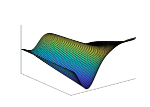
Figure 8. The unstable spanwise mode pair in the eigenspectrum of the problem at $Pr=0.001$, $k=0$, $m=0.3$, $Ra=55$, $\eta =1$ and ${Bi=10^{-5}}$. These modes become unstable for $Pr<1$ and possess the same growth rate travelling in the opposite directions with the same phase speed.

5.1. Energy budget analysis

To understand the origins of the new mode of instability emerging for $Pr<1$, we carry out an energy budget analysis for the case of two-dimensional ($m=0$) perturbations and follow the approach used by Hu, He & Chen (Reference Hu, He and Chen2016), Hu et al. (Reference Hu, He, Chen and Liu2017) and Patne et al. (Reference Patne, Agnon and Oron2021a).

First, the Navier–Stokes equations in the Boussinesq approximation (2.2b) are linearized around the base state $\bar {\boldsymbol {v}}, \bar p, \bar T,$ and recast in the form

(5.1)\begin{equation} \frac{1}{Pr} \frac{\partial \boldsymbol{v}^\prime}{\partial t} ={-}\boldsymbol{\nabla} p^\prime + \boldsymbol{\nabla} \boldsymbol{\cdot} \boldsymbol{\tau}^\prime + Ra \,T' \boldsymbol{\nabla} y - \frac{1}{Pr} \left[ (\boldsymbol{v'} \boldsymbol{\cdot}\boldsymbol{\nabla}) \bar{\boldsymbol{v}} + (\bar{\boldsymbol{v}} \boldsymbol{\cdot}\boldsymbol{\nabla}) \boldsymbol{v'} \right], \end{equation}

where $\boldsymbol {\tau }^\prime$ is the disturbance of the stress tensor for a Newtonian fluid. Taking the scalar product of (5.1) with the perturbation velocity vector ${\boldsymbol v}^\prime$, integrating the result over the flow domain and simplifying the resulting integrals yields an equation describing the time evolution of the total kinetic energy of the perturbations,

(5.2)\begin{equation} E= \frac12 \int{ {\boldsymbol v}^\prime \boldsymbol{\cdot} {\boldsymbol v}^\prime\,{\rm d} V}, \end{equation}

in the form

(5.3)\begin{align} \frac{1}{Pr} \frac{\partial E}{\partial t} &={-} \frac{1}{2} \int \boldsymbol{\tau}^\prime : \boldsymbol{\dot{\gamma}^\prime}\,{\rm d} V + Ra \int T' v'_y \,{\rm d} V - \frac{1}{Pr} \int \boldsymbol{v'} \boldsymbol{\cdot} \boldsymbol{\bar{\dot{\gamma}} } \boldsymbol{\cdot} \boldsymbol{v'} \,{\rm d} V \nonumber\\ &\equiv{-} I_b + I_{RB} - I_R, \end{align}

where ${I_b}$, $I_{RB}$ and $I_{R}$ are the bulk stress work, Rayleigh–Bénard integral or buoyancy work and the Reynolds stress work (Drazin Reference Drazin2002) in the energy balance, respectively, ${\rm d}V$ is the volume element and $\dot {\boldsymbol {\gamma }}^\prime = \boldsymbol {\nabla } \boldsymbol {v}^\prime + \boldsymbol {\nabla } {\boldsymbol {v}^\prime }^{\rm T}$ and $\boldsymbol {\bar {\dot {\gamma }}}= \boldsymbol {\nabla } \bar {\boldsymbol {v}} + \boldsymbol {\nabla } \bar {\boldsymbol {v}}^{\rm T}$ represent the strain-rate tensors associated with the perturbed and base states, respectively.

Since the perturbations of the normal component of the velocity field ${\boldsymbol v}^\prime$ vanish at both non-deformable interfaces, namely the free interface $y=1$ and the liquid–solid interface $y=0$, the pressure work term in the energy balance equation (5.3) containing area integrals evaluated at these two interfaces vanishes, and thus is not presented there explicitly. Therefore, unlike the energy budget in the case of thermocapillary instability (Patne et al. Reference Patne, Agnon and Oron2021a), the pressure work does not contribute here. Some sample values of the various terms in (5.3) are shown in table 1. The buoyancy work term $I_{RB}$ in (5.3) is found to be positive for the parameter values explored here; thus it exerts a destabilizing effect. The bulk stress work component $I_b$ is unconditionally positive in the case of a Newtonian fluid, since $\boldsymbol {\tau }^\prime : \dot {\boldsymbol {\gamma }}^\prime = \gamma '_{ij}\gamma '_{ji} \ge 0$, and thus leads to a decrease in the perturbation energy expressing the presence of viscous dissipation. Note that the long-wave mode for $\eta =0$ may emerge even if the bulk stress work integral is positive. These long-wave modes may become unstable due to the energy supplied by the buoyancy work $I_{RB}$ that overcomes the stabilizing impact of the dissipation factors such as viscous forces and thermal diffusion of the energy.

Table 1. Sample values of the bulk stress work $I_b$ and Reynolds stress work $I_R$ components in the energy balance equation (5.3) normalized by the value of the buoyancy work $I_{RB}$ for $Bi=0.001$, $m=0$ and $Pr=0.001$ in the case of the unstable stationary long-wave mode (the first row) and the new modes (the last two rows). The bulk stress work remains positive as expected, and hence has a stabilizing effect driven by the viscous dissipation. The Reynolds stress work is negative and increases rapidly with an increase in $\eta$, which results in the growth of the perturbation energy. Therefore, the main source of destabilization for the new mode is the Reynolds stress work.

The Reynolds stress work $I_R$ in the energy balance equation (5.3) represents a volume-averaged correlation between the perturbations in the horizontal and vertical components of the velocity field. This term is also responsible for the energy exchange between the base state and the perturbation fields. It must be noted that $I_R$ is found to be negative for the parameter range studied here. The role of the Reynolds stress work is enhanced at low values of $Pr$ and high values of $\eta$. It follows from table 1 where all values of the integrals are normalized with respect to the buoyancy work term $I_{RB}$, that the contribution of the latter to the energy balance is the main source of the perturbation energy for the long-wave mode, as seen in the first row of table 1. However, as follows from the last two rows of table 1, the contribution of the buoyancy work term $I_{RB}$ to the perturbation energy for the new mode becomes less important with an increase in $\eta$.

As shown in figure 7(b), the new mode bifurcates from the long-wave mode at $\eta \sim 0.005$ and table 1 illustrates that the Reynolds stress work and the buoyancy work are of comparable magnitudes for $\eta =0.01$. Thus, the buoyancy work also significantly contributes to the destabilization of the new mode in the low-$\eta$ domain, but its influence diminishes with an increase in $\eta$. To conclude, the major sources of the perturbation energy for the long-wave and the new modes are the buoyancy work and the Reynolds stress work, respectively. However, the emergence of the new modes for $Pr<1$ is associated with the rise in the Reynolds stress work.

It must be noted that the perturbation energy analysis carried out here can only provide an idea about perturbation energy sources that may lead to destabilization (Drazin Reference Drazin2002). However, the right critical parameter values may be obtained only using the GLSA.

5.2. Physical mechanism

The physical mechanism responsible for the onset of buoyancy-driven or Rayleigh–Bénard convection in a liquid layer subjected to a purely VTG is well understood. Given that the substrate is at a higher temperature compared to the liquid–gas interface, a negative VTG is imposed across the layer. Consider a liquid parcel located at $y=y_0$. Due to the imposed VTG, the density of the liquid parcel located at $y=y_0$ will be lower compared with that of the liquid layer present at $y=y_0+{\rm \Delta} y$, where ${\rm \Delta} y>0$ is a small quantity. In the presence of the gravity field, the liquid parcel will thus try to move to $y=y_0+{\rm \Delta} y$. Such a motion will be opposed by the dissipative effects such as viscosity and thermal diffusion of the liquid, but if the VTG strength is sufficiently strong, then the parcel can overcome the dissipative effects combined and succeed in moving to $y=y_0+{\rm \Delta} y$ owing to the buoyancy forces, thereby setting in the buoyancy-driven instability. Having understood the physical mechanism of the buoyancy-driven instability caused by the purely imposed VTG, we now proceed to understand the effect of the imposed HTG on the VTG-induced convection and the origin of the new mode of instability.

5.2.1. Long-wave mode stabilization

In § 4, we illustrated the strong stabilizing effect of the imposed HTG on the long-wave mode introduced by the imposed VTG. The physical consequences of such stabilization can be understood as follows. It is inferred from (2.12b) that along with the imposed VTG, the latter also gives rise to an induced VTG which has a quartic polynomial form in $y$. The average total VTG defined as $\langle {\bar T}_y \rangle \equiv \int _0^1 {(\partial {\bar T}/\partial y)\,{{\rm d}y}}$ is thus

(5.4)\begin{equation} \langle{\bar T}_y \rangle= \frac{\eta^2 Ra}{320}-1, \end{equation}

which shows that the induced VTG being positive always opposes the imposed VTG.

As discussed in the previous section, for the buoyancy instability to set in the buoyancy forces must overcome the viscous forces and thermal diffusion of the energy. However, the induced VTG opposes the imposed VTG, which leads to the weakening in the total VTG. The buoyancy force caused by the weakened VTG may not be sufficient to overcome the viscous forces and thermal diffusion of the energy which then leads to the predicted stabilization with an increase in $Ra$. When the vertically averaged imposed and induced VTGs are of equal magnitude, the average VTG vanishes, which yields the relationship $Ra=320/\eta ^2$, thereby defining the upper bound on the threshold of the long-wave instability, which turns out to be valid for very low values of the Biot number $Bi$, as indeed shown in the case presented in figure 4. However, for higher but still low values of $Bi$, the instability may still exist for a positive averaged total VTG, as shown in figure 5.

5.2.2. New mode

As discussed in § 5, the maximal contribution to the perturbation energy for the new mode arises from the Reynolds stress work which involves a $1/Pr$ term. Thus, with a decrease in $Pr$, the contribution of the Reynolds stress work increases with a further destabilization of the base flow. A decrease in $Pr$ implies an enhancement of the inertial effects as seen from (5.1). Additionally, the condition of $Pr<1$ for the emergence of the new mode emphasizes the major role of inertia. The normalized perturbation fields for the new mode are shown in figure 9. The temperature perturbation field exhibits variation through the entire liquid layer; however, the normal velocity perturbation exhibits the maximal variation evaluated by the absolute value of the gradient vector at $y \sim 0.578$ and vanishes at both ends. The base-state velocity $\bar v_x$ vanishes at $y \sim 0.578$ being positive for $y>0.578$ and negative for $y<0.578$; therefore there exists a static layer arising as a result of the opposing shear stresses exerted by the forward ($\bar v_x>0$) and return ($\bar v_x<0$) flows. As a result, there exists a velocity jump over a thin layer at $y\sim 0.578$, which is known to be responsible for various kinds of instabilities (Hinch Reference Hinch1984). Here, such a jump could result in the emergence of the new mode of instability provided that the inertial effects are sufficiently strong. To conclude, the new mode of instability revealed here may emerge as a result of the velocity jump in the liquid layer.

Figure 9. Normalized perturbation fields for ${Bi=10^{-5}}$, $Pr=0.001$, $\eta =1$, $Ra=7.5$, $m=0$ and $k=0.38$ for the marginally stable eigenvalue $\omega =0.055044$. Here, (a) $v'_x=Re[ \tilde v_x \,{\rm e}^{{\rm i}kx}]$, (b) $v'_y=Re[\tilde v_y \,{\rm e}^{{\rm i}kx}]$ and (c) $T'=Re[\tilde T\,{\rm e}^{{\rm i}kx}]$. The length of the domain in the $x$ direction is equal to the wavelength of the perturbations $2{\rm \pi} /k$. For convenience, the axes are normalized to the interval $[0,1]$. The normal velocity perturbation field (b) exhibits the maximal variation in the layer and vanishes at both boundaries providing a hint for the destabilization mechanism of the new mode.

6.1. Derivation of the evolution equation

In the governing equations (2.2), the dependent variables are expressed as $v_x=\bar v_x + v^\prime _x$, $v_y= v^\prime _y$, $p=\bar p+p^\prime$ and $T=\bar T + T^\prime$ to obtain the equations in terms of the deviations from the base state:

(6.1a)$$\begin{gather} \partial_x v^\prime _x+ \partial_y v^\prime_y=0, \end{gather}$$

(6.1b)$$\begin{gather}\frac{1}{Pr} \left[ \partial_t v^\prime_x + (\bar v_x + v^\prime_x) \partial_x v^\prime_x + v^\prime_y \partial_y (\bar{v}_x+v^\prime_x)\right] ={-}\partial_x p^\prime + (\partial_x^2+\partial_y^2) v^\prime_x, \end{gather}$$

(6.1c)$$\begin{gather}\frac{1}{Pr} \left[ \partial_t v^\prime_y + (\bar v_x + v^\prime_x) \partial_x v^\prime_y + v^\prime_y \partial_y v^\prime_y \right] ={-}\partial_y p^\prime + (\partial_x^2+\partial_y^2) v^\prime_y +Ra T^\prime, \end{gather}$$

(6.1d)$$\begin{gather}\partial_t T^\prime + (\bar v_x + v^\prime_x) \partial_x T^\prime + v^\prime_y \partial_y \left(\bar T+ T^\prime \right) = (\partial_x^2+\partial_y^2) T^\prime, \end{gather}$$

where the dependent variables with primes represent the above-mentioned respective deviations. Similarly, the boundary conditions (2.3e) are modified to read: at $y=0$, no slip, no impermeability and a specified temperature gradient at the lower plate imply

(6.2a)\begin{equation} v^\prime_x=0; \quad v'_y=0; \quad v'_z=0; \quad \partial_y T' =0. \end{equation}

At $y=1$, the kinematic boundary condition, zero tangential stress and the heat transfer condition become

(6.2b)$$\begin{gather} v'_y=0, \end{gather}$$

(6.2c)$$\begin{gather}\partial_x v'_y + \partial_y v'_x=0, \end{gather}$$

(6.2d)$$\begin{gather}\partial_y T' + Bi \, T'=0. \end{gather}$$

The deviation velocities are further expressed via the streamfunction $\psi$ using the relations

(6.3a,b)\begin{equation} v^\prime_x= \partial_y \psi; \quad v^\prime_y={-}\partial_x \psi. \end{equation}

As noted above, we assume small values of $\eta$, $\eta = \epsilon \hat {\eta }$, so that $\hat \eta = O(1)$ and $\epsilon \ll 1$ is a smallness scale of $\eta$ used hereafter as a small expansion parameter in the asymptotic analysis. The following scaling is applied:

(6.4a–e)\begin{equation} \xi = \epsilon x; \quad \tau = \epsilon^4 t; \quad \psi= \epsilon \hat{\psi}; \quad T'= \hat{T};\quad Bi = \epsilon^4 \widehat{Bi}, \end{equation}

with a hat used to denote a scaled value. Equations (6.4a–e) are then substituted into the governing equations (6.1) and the boundary conditions (6.2), the pressure field is eliminated from the equations and these are modified using (6.3a,b). Furthermore, the scaled streamfunction, the temperature and the Rayleigh number are expanded as

(6.5a)$$\begin{gather} \hat{\psi} = \psi_0 + \epsilon^2 \psi_2 + \epsilon^4 \psi_4 + \cdots, \end{gather}$$

(6.5b)$$\begin{gather}\hat{T} = T_0 + \epsilon^2 T_2 + \epsilon^4 T_4 + \cdots, \end{gather}$$

(6.5c)$$\begin{gather}Ra = Ra_0 + \epsilon^2 \widehat{Ra}_2 + \epsilon^4 \widehat{Ra}_4 + \cdots. \end{gather}$$

Following elimination of pressure, (6.1) are rewritten along with (6.5) to yield at zero-order approximation in $\epsilon$

(6.6a,b)\begin{equation} \partial_y^4\psi_0 + Ra_0 \partial_\xi T_0=0; \quad \partial_y^2 T_0=0. \end{equation}

The boundary conditions are similarly simplified. Given the linear form of the boundary conditions in the present problem, for the sake of brevity, we do not write out the boundary conditions in the following analysis since they are readily obtained from (6.2) by substituting expansions (6.5).

Equations (6.6a,b) admit the solution for $\psi _0$ and $T_0$ in the form

(6.7a,b)\begin{equation} T_0= F(\xi,\tau); \quad \psi_0= \frac{Ra_0}{48} (3 y^2 - 5 y^3 + 2 y^4) \partial_\xi F, \end{equation}

where $F(\xi,\tau )$ is an unknown function at this stage whose governing evolution equation is now being derived to determine the spatio-temporal dynamics of the system. We remind the reader that $F$ represents the leading order in $\epsilon$ perturbation of the base-state temperature field.

Similarly, the bulk equations (6.1) at $O(\epsilon ^2)$ read

(6.8a)\begin{align} & -48Pr \partial_y^4 \psi_2 + 6 \hat \eta Ra_0 (8y-5) \partial_\xi \psi_0 + 48 Pr \,\widehat{Ra}_2 (\partial_\xi F +\partial_\xi T_2) \nonumber\\ &\quad + \hat \eta Ra_0 y({-}6+15y-8y^2) \partial_\xi \partial_y^2 \psi_0 - 96 Pr \partial_\xi^2 \partial_y^2 \psi_0=0, \end{align}

(6.8b)\begin{align} & \partial_y^2 T_2 + \partial_\xi^2 F- \partial_\xi \psi_0 +{-} \partial_\xi F\partial_y \psi_0 \nonumber\\ &\quad + \hat \eta Ra_0 \left(\frac{1}{8} y - \frac{5}{16} y^2 + \frac{1}{6} y^3 \right)\partial_\xi F=0. \end{align}

Using the appropriate boundary conditions at $O(\epsilon ^2)$, the above equations are then solved.

To obtain the value for $Ra_0$, (6.8b) is integrated with respect to $y$ across the layer $y \in (0,1)$ using the boundary conditions at $O(\epsilon ^2)$. The resulting equation is then solved for $Ra_0$ to yield $Ra_0 = 320$, which is in excellent agreement with $Ra_c=320$ obtained from the numerical solution for a liquid layer subjected to a purely VTG in § 4, thereby validating the accuracy of the numerical approach. Also note that Gertsberg & Sivashinsky (Reference Gertsberg and Sivashinsky1981) find that in the case of a layer bounded by two solid walls, $Ra_c=720$. A lower value of the critical Rayleigh number $Ra_c$ here is due to the fact that the case of solid wall-free surface features less dissipation in the presence of one solid boundary, as compared to the case of a layer bounded by two solid walls. Therefore, the system needs a lower value for $Ra$ for instability to set in.

The solution of (6.8) satisfying the appropriate boundary conditions at second order in $\epsilon$ is

(6.9a)\begin{align} \psi_2 &= \frac{y^2}{9072 Pr} (Pr \partial_\xi F (189 \widehat{Ra}_2 (y-1) (2y-3) \nonumber\\ &\quad +320 (435 - 505 y + 2 y^5 (72 -45 y + 8 y^2)) \partial_\xi^2 F ) \nonumber\\ &\quad + 32 (1890 Pr ({-}1 + y) ({-}3 + 2 y) \partial_\xi G - 5 \hat \eta (177 - 347 y \nonumber\\ &\quad +2 Pr (435 - 505 y + 2 y^5 (72 -45 y+ 8 y^2)) \nonumber\\ &\quad + 2 y^3 (378 -630 y+ 522 y^2 -225 y^3+ 40 y^4)) \partial_\xi^2 F \nonumber\\ &\quad + Pr (90 + y (240 -945 y + 945 y^2- 378 y^3 + 90 y^5 - 50 y^6 + 8 y^7)) \partial_\xi^3 F )), \end{align}

(6.9b)\begin{align} T_2 &= G(\xi,\tau) - \frac{6 y^3}{18} (20-25y+8y^2)(2 \hat \eta - \partial_\xi F)\partial_\xi F \nonumber\\ &\quad + \frac{y^2}{18} (8y^6 - 30 y^5 + 30 y^4 - 9 y^2) \partial_\xi^2 F, \end{align}

where $G(\xi,\tau )$ is an unknown function, which turns out to be irrelevant for the evolution of the system up to $O(\epsilon ^4)$.

At $O(\epsilon ^4)$, the energy equation reads as

(6.10)\begin{align} & -\partial_\tau F+ \hat \eta \partial_y \psi_ 2 + \partial_y^4 T_ 2 + 20 \hat \eta^2 y^2 \partial_\xi \psi_ 0 - \tfrac{100}{3} \hat \eta^2 y^3 \partial_\xi \psi_ 0 \nonumber\\ &\quad +\tfrac{40}{3}\hat \eta^2 y^4 \partial_\xi \psi_ 0 + \partial_y T_ 2 \partial_\xi \psi_ 0 - \partial_\xi \psi_ 2 + \tfrac{1}{8} \hat \eta \widehat{Ra}_2 y \partial_\xi F \nonumber\\ &\quad - \tfrac{5}{16} \hat \eta \widehat{Ra}_2 y^2 \partial_\xi F + \tfrac{1}{6} \hat \eta \widehat{Ra}_2 y^3 \partial_\xi F - \partial_y \psi_ 2 \partial_\xi F+ 40 \hat \eta y \partial_\xi F \nonumber\\ &\quad - 100 \hat \eta y^2 \partial_\xi T_ 2 + \tfrac{160}{3} \hat \eta y^3 \partial_\xi T_ 2 - \partial_y \psi_ 0 \partial_\xi F+ \partial_\xi^2 T_ 2=0. \end{align}

To obtain the governing evolution equation for $F(\xi,\tau )$, the solution at $O(\epsilon ^2)$ given by (6.9) needs to be substituted into (6.10), and the latter is integrated with respect to $y$ across the layer $y \in (0,1)$ along with the appropriate boundary conditions. As a result, we obtain the governing evolution equation for $F(\xi,\tau )$ in the form

(6.11)\begin{align} & \partial_\tau F + \frac{58}{693} \partial_\xi^4 F - \left[\frac{1}{6} \hat \eta +\frac{5 \hat \eta}{42 Pr} \right]\partial_\xi^3 F + \frac{1}{12} \partial^2_\xi \left[\left(\partial_\xi F\right)^2\right] \nonumber\\ &\quad + \left[ -\frac{760}{189} \hat \eta^2 +\frac{1}{320} \widehat{Ra}_ 2 + \frac{1520}{189} \hat \eta \partial_\xi F - \frac{760}{189} (\partial_\xi F )^2\right]\partial_\xi^2 F + \widehat{Bi}\, F=0, \end{align}

where the Biot number term $\widehat {Bi} F$ arises due to the heat transfer boundary condition at the free surface $y=1$ at $O(\epsilon ^4)$. Before proceeding further we scale out $\epsilon$ from the above equation by using the scaling (6.4a–e) expressing the system dynamics in terms of the unscaled dimensionless variables and parameters to obtain

(6.12)\begin{align} & \partial_t F + \frac{58}{693} \partial_x^4 F -\eta \left[ \frac{1}{6} + \frac{5}{42 Pr} \right]\partial_x^3 F \nonumber\\ &\quad + \partial_x \left[\left(\frac{1}{320} Ra_2 -\frac{760}{189} \eta^2 + \frac{760}{189} \eta \partial_x F - \frac{760}{567} (\partial_x F )^2 + \frac{1}{6} \partial^2_x F\right) \partial_x F\right] + Bi F = 0, \end{align}

where $Ra_2 = \epsilon ^2 \widehat {Ra}_2$. The analyses below are carried out based on the evolution equation (6.12).

6.2. Linear stability analysis

To carry out the linear stability analysis of the base state corresponding to $F=0$, we substitute $F(x,t) = \zeta \exp ({{\rm i} (k x-\omega t)})$ into (6.12) where $\zeta \ll 1$ is an arbitrary constant. Upon linearization and further simplification, we obtain the dispersion relation

(6.13)\begin{equation} \omega= \frac{\eta k^3 (5 + 7 Pr)}{42 Pr} +{\rm i}\left[{-}Bi + R k^2 - \frac{58 k^4}{693} \right], \end{equation}

where

(6.14)\begin{equation} R=\frac{Ra_2}{320}-\frac{760 \eta^2}{189}. \end{equation}

The real and imaginary parts of (6.13) are

(6.15a)$$\begin{gather} \omega_r = \frac{\eta k^3 (5 + 7 Pr)}{42 Pr}, \end{gather}$$

(6.15b)$$\begin{gather}\omega_i ={-} Bi +R k^2 - \frac{58 k^4}{693}. \end{gather}$$

The variation of the growth rate $\omega _i$, i.e. the imaginary part of $\omega$, as a function of the wavenumber $k$ with an increase in $\eta$ is presented in figure 10. In agreement with the GLSA, an increase in the HTG $\eta$ has a strong stabilizing effect on the long-wave mode introduced by the VTG.

Figure 10. Variation of the growth rate $\omega _i$ with the wavenumber $k$ at $Bi=0.001$, $Pr=10$ and $Ra_2=16$ for various $\eta$ as given by (6.15b). The figure illustrates a strong stabilizing effect of the increase in the relative strength of the HTG $\eta$ on the long-wave mode induced by the imposed VTG.

Since at $k =0$ the growth rate $\omega _i=-Bi$ is negative and in the limit of $k \to \infty$ the growth rate $\omega _i \sim -k^4$ is also negative, the stability properties of the system are determined via the sign of the maximal value of $\omega _i$ in the intermediate range. This leads to the result that along the neutral stability curve, i.e. $\omega _i = 0$,

(6.16)\begin{equation} Ra_2 = \tfrac{243\,200}{189} \eta^2 +640 \sqrt{\tfrac{58}{693}Bi}. \end{equation}

The critical Rayleigh number up to $O(\epsilon ^2)$ correction is thus

(6.17)\begin{equation} Ra_c = Ra_0 + Ra_2 = 320 + \tfrac{243\,200}{189} \eta^2 +640 \sqrt{\tfrac{58}{693}Bi}. \end{equation}

This clearly illustrates the stabilizing effect of an increase in $\eta$ via an increase in the critical Rayleigh number $Ra_c$ on the long-wave mode in agreement with the GLSA.

Similarly, the effect of an increase in the Biot number $Bi$ is also stabilizing, as seen in figure 11, which presents the variation of the growth rate $\omega _i$ with the wavenumber $k$ and the Biot number $Bi$ for $\eta =0$ and $Ra_2=16$ representing $5\,\%$ supercriticality. Due to the presence of heat transfer at the free surface, $Bi \neq 0$, the long-wave mode $k \to 0$ is linearly stable. Similarly, short waves are damped due to dissipation promoted by viscosity and thermal diffusivity of the liquid, $\omega _i < 0$ for $k \gg 1$. This leaves an intermediate (still long-wave) range of the disturbance wavenumber $k$ to exhibit instability $\omega _i>0$, and gives rise to the emergence of two values of $k$, $k=k_1 \approx 0.133$ and $k = k_2 \approx 0.774$ for $Bi=0.001$, where the growth rate $\omega _i$ vanishes. The fastest growing linear mode $k=k_m$ is determined as usual via solution of the equation ${\rm d}\omega _i / {\rm d} k =0$, which yields in the case of $Bi=0.001$, $k=k_m \approx 0.5465$. We refer to this figure below in discussion of the results in the context of nonlinear dynamics of the system revealed via numerical solution of the evolution equation (6.12).

Figure 11. Growth rate $\omega _i$ as a function of the wavenumber $k$ for $Ra_2=16$ and $\eta =0$ as given by (6.15b) for different $Bi$. Note that the growth rate $\omega _i$ is independent of the Prandtl number $Pr$.

Figure 12 displays a comparison of $Ra_c$ obtained from both the numerical and long-wave analyses. An excellent agreement between the two approaches for $\eta <0.2$ proves the validity of the long-wave asymptotic analysis. It is noteworthy that, as follows from (6.17), the maximal value of the second-order correction is ${\approx }31.5$ for $\eta <0.1$ and $Bi \le 0.01$, which is much smaller (about $10\,\%$) than $Ra_0=320$.

Figure 12. Variation of $Ra_c$ with $\eta$ at $Pr=10$ and ${Bi=10^{-5}}$. Along the lower branch, the analytically obtained value of $Ra_c$ given by (6.17) is in excellent agreement with the values of $Ra_c$ determined numerically for $\eta <0.2$, thereby validating the former.

6.3. Spatio-temporal linear stability analysis

In this subsection, for the sake of simplicity, we present the results for the case of $Bi=0$, which remain practically unaffected for small but non-zero $Bi$ ($< O(10^{-4})$). To carry out the temporal stability analysis, $\omega$ is taken as a complex number, while the wavenumber $k$ is treated as a real number (Drazin & Reid Reference Drazin and Reid1981). To investigate the spatial stability analysis aimed at determining the evolution of disturbances in space, the frequency $\omega$ is treated as a real number while $k$ is a complex number (Drazin Reference Drazin2002). Conversely, in a spatio-temporal stability analysis, both $\omega$ and $k$ are treated as complex numbers (Huerre & Monkewitz Reference Huerre and Monkewitz1990; Schmid & Henningson Reference Schmid and Henningson2001). This section is aimed at understanding the impact of the HTG on the emergence of absolute instability.

An instability is classified as either absolute or convective if the growth of disturbances takes place in both upstream and downstream directions or the disturbances develop in the downstream direction from their source, respectively (Briggs Reference Briggs1964; Huerre & Monkewitz Reference Huerre and Monkewitz1990; Schmid & Henningson Reference Schmid and Henningson2001). The proposed methodology to determine the existence of absolute instability is by progressively moving the Laplacian contour in the $\omega _r$–$\omega _i$ plane and the Fourier contour in the $k_r$–$k_i$ plane (Briggs Reference Briggs1964).

Thus, in the case of convective instability, the disturbances will decay at any fixed position in space if sufficient time is allowed for that (Huerre & Monkewitz Reference Huerre and Monkewitz1990). This results in mixing in the downstream direction only, whereas absolute instability will induce mixing in both upstream and downstream directions. The emergence of absolute or convective instability can be illustrated by considering the response of a given base velocity profile to an impulse excitation at asymptotically long times (Huerre & Monkewitz Reference Huerre and Monkewitz1990).

The emergence of absolute instability for a given dispersion relation $\omega =g(k)$ with a continuous and differentiable function $g(k)$ can be detected if the group velocity of the disturbances has at least one saddle point, i.e. there exists at least one root $k$ for the equation ${\partial \omega }/{\partial k}=0$ (Huerre & Monkewitz Reference Huerre and Monkewitz1990; Schmid & Henningson Reference Schmid and Henningson2001). However, the determined saddle point must also obey the causality principle for the existence of absolute instability (Huerre & Monkewitz Reference Huerre and Monkewitz1990).

To obtain a sufficient condition for the emergence of absolute instability, the equation ${\partial \omega }/{\partial k}=0$ is solved in terms of $k$, which yields the saddle points of the dispersion relation. If the saddle point $k=k_0$ is of first order in the $k$ plane, then a local Taylor expansion for $\omega$ about this point yields $(\omega -\omega _{0})\sim (k-k_{0})^{2}$, where $\omega _0 \equiv \omega (k_0)$. This shows that the mapping from the $k$ plane ($k=k_r+{\rm i}k_i$) to the $\omega$ plane $(\omega =\omega _r+{\rm i}\omega _i$) for a first-order saddle point is characterized by angle doubling. Note that the $k$ and $\omega$ planes are spanned over $k_r$–$k_i$ and $\omega _r$–$\omega _i$, respectively.

For realistic dispersion relations, finding a saddle point in the $k$ plane and a cusp point in the $\omega$ plane according to the method of Briggs (Reference Briggs1964) becomes a cumbersome mathematical and numerical task. A simpler alternative is the method of Kupfer, Bers & Ram (Reference Kupfer, Bers and Ram1987), in which for a prediction of absolute instability, only the formation of a cusp point in the $\omega$ plane is necessary. Figure 13 illustrates a genuine cusp point in the $\omega$ plane, thereby illustrating the existence of absolute instability for a non-zero $\eta$.

Figure 13. Cusp point formation at $Pr=7$, $Ra_2=25$, $\eta =0.1$ and $Bi=0$. The figure illustrates the existence of absolute instability for a non-zero $\eta$ in the $\omega _r$–$\omega _i$ plane. The cusp point is located at $\omega _{0} = 0.00189 + 0.00379{\rm i}$. A straight curve drawn from the cusp point $\omega =\omega _{0}$ intersects the $k_i=0$ curve once, i.e. an odd number of times, thereby confirming the genuine nature of the cusp point. The cusp point corresponds to $\omega _{i0}>0$; thus for the chosen parameter set, the system is absolutely unstable.

For $\eta =0$, (6.13) yields $\omega _r=0$; thus disturbances do not travel and $\omega _i>0$ for $Ra_2>0$ for a range of sufficiently low $k$. Thus, in the absence of the imposed HTG, the flow is absolutely unstable and the critical Rayleigh numbers for the onset of the temporal and absolute instabilities are equal. However, for $\eta >0$, $\omega _r \neq 0$, and the flow may become convectively unstable as illustrated in figure 14.

Figure 14. Cusp point formation in the case of $Pr=7$, $Ra_2=14$, $\eta =0.1$ and $Bi=0$. The cusp point is located at $\omega _{0} = 3.1626 \times 10^{-5} - 2.9339 \times 10^{-7}{\rm i}$, and corresponds to $\omega _{i0}<0$; thus the system with a given parameter set is convectively unstable.

Given a simple structure of the dispersion relation (6.13), the location of a saddle point in the $k$ plane and that of a cusp point in the $\omega$ plane is readily obtained. Differentiating (6.13) with respect to $k$ once and then solving the equation ${\rm d}\omega /{\rm d} k=0$ yields a saddle point:

(6.18)\begin{align} k_0 &={-}{\rm i}\frac{1485 \eta (5 + 7 \,Pr)}{13\,920 \,Pr} \nonumber\\ &\quad +\frac{\sqrt{3\,617\,460 \,Pr^2 \,Ra_2 -825 \eta^2 \left[66\,825 + Pr (187\,110 + 5\,773\,217 Pr)\right] }}{13\,920 \,Pr}. \end{align}

A mirror saddle point with $k_r<0$ and the same $k_i$ also exists as the second solution of the equation ${\partial \omega }/{\partial k}=0$. Since we consider now a solution with $k_r>0$ only, the saddle point with $k_r<0$ will not be used henceforth. It must be noted that the saddle point with $k_r<0$ corresponds to the cusp point with $\omega _r<0$ and both saddle points will yield the same value of $\omega _{i0}$. We now substitute $k=k_0$ into (6.13) and obtain the corresponding value $\omega _0 =\omega (k_0)$. The variation of the critical parameters for the emergence of the temporal and absolute instabilities and the value of $k_{i0}$ is shown in figure 15. For example, for $\eta =0.1$, the critical values for $Ra_2$ in the cases of the temporal and absolute instabilities are ${\sim }12.88$ and ${\sim }14.1$, respectively. Also, with $\eta =0$, the critical values $Ra_2$ for the emergence of the temporal and absolute instabilities are equal to zero.

Figure 15. Variation of the critical parameters at $Pr=7$ and $Bi=0$. (a) The difference between the critical $Ra_2$ for the thresholds of the temporal and absolute instabilities and $k_{i0}$ increases with an increase in $\eta$, thereby showing the role of the imposed HTG in the emergence of convective instability. (b) A magnified part of (a) to emphasize the existence of the convectively unstable streamwise mode.

Variation of the cusp point location in the $\omega$ plane with the Prandtl number $Pr$ is presented in figure 16. It follows from the governing equations (2.2b) that with a decrease in $Pr$, the inertial terms become more important. This leads to a stronger convection, thereby even resulting in the convective instability at sufficiently low $Pr$. On the other hand, as $Pr$ increases, the flow becomes absolutely unstable with a rapid initial rise in the growth rate $\omega _i$ until $Pr\sim 0.2$ where the latter achieves a constant value which remains the same with a further increase in $Pr$.

Figure 16. Variation of the cusp point location ($\omega _0=\omega _{r0}+{\rm i} \omega _{i0}$) with $Pr$ at $Ra_2=20$, $\eta =0.01$ and $Bi=0$.

6.4. Weakly nonlinear analysis

Similar to the previous subsection, for the sake of simplicity, we present the results in the case of $Bi=0$ which remain practically unaffected for small but non-zero $Bi$ ($< O(10^{-4})$). To carry out the weakly nonlinear stability analysis, we follow the approach used by Cheng, Chen & Lai (Reference Cheng, Chen and Lai2001), Oron & Bankoff (Reference Oron and Bankoff1999) and Patne et al. (Reference Patne, Agnon and Oron2021a) and introduce slow time scales $T_1=\delta t, T_2=\delta ^2 t$, where $\delta \ll 1$ is a small parameter related to the deviation of the Rayleigh number $Ra$ from its critical value $Ra_{c}$ via (6.19a). The Rayleigh number $Ra$ and the temperature disturbance $F(x,t)$ are expanded into series of $\delta$ as

(6.20a)$$\begin{gather} Ra_2=Ra_{2c} (1 + \delta^2), \end{gather}$$

(6.20b)$$\begin{gather}F(x,t) = 1+ \delta F_1 (x,t,T_1,T_2) + \delta^2 F_2 (x,t,T_1,T_2)+ \delta^3 F_3 (x,t,T_1,T_2)+\cdots, \end{gather}$$

where $Ra_{2c}$ is the critical value of the Rayleigh number obtained by solving (6.15b) for $\omega _i=0$ with $k=k_c=2 {\rm \pi}/L$ being the cut-off wavenumber and $L$ the length of the periodic domain, namely

(6.21)\begin{equation} {-}Bi +\left(\frac{Ra_{2c}}{320}-\frac{760 \eta^2}{189}\right)k_c^2 -\frac{58}{693}k_c^4=0. \end{equation}

These are substituted into (6.12). The problem is then solved order by order in $\delta$ in terms of $F_i$.

At first order in $\delta$, the correction to the temperature disturbance $F_1$ due to the perturbations is obtained in the form

(6.19)\begin{equation}F_1 (x,t,T_1,T_2)= a(T_1,T_2) \exp {({\rm i} (k_c x - \omega _r t))} + {\rm c.c.},\end{equation}

where $a(T_1,T_2)$ is the complex amplitude of the perturbation, yet unknown, evolving in slow time and c.c. denotes complex conjugate. At second order in $\delta$, the solvability condition yields that the complex amplitude $A$ is independent of the slow time scale $T_1$, namely $A=A(T_2)$. Also, the solution of the differential equation at second order is exponential similar to $F_1$ above, namely $F_2 (x,t,T_1,T_2)= b(T_2) \exp [(2{\rm i} (k_c x -\omega _r t)] + {\rm c.c.}$ with the complex amplitude $b(T_2)$ proportional to $a(T_2)^2$.

Finally, at third order in $\delta$, the Landau equation governing the temporal evolution of the amplitude function $a \equiv a(T_2)$ in slow time $T_2$ is obtained:

(6.22a)\begin{equation} \partial_{T_2} a=\lambda_1 a + \lambda_2 |a|^2 a, \end{equation}

where $\lambda _1$ and $\lambda _2$ are the Landau parameters:

(6.22b)\begin{equation} \lambda_1=\delta^{{-}2}k_c^2\left(Ra_2-Ra_{2c}\right),\quad \lambda_2 = \frac{\lambda_{2n}}{\lambda_{2d}}-\frac{760}{189} k_c^4, \end{equation}

where

(6.22c)\begin{equation} \lambda_{2n}=880 (1520 \eta + 63 {\rm i} k_c) (3040 \eta + 63 {\rm i} k_c) k_c^6 Pr, \end{equation}

(6.22d)\begin{align} \lambda_{2d} &= 189 [320k_c^2 (8360 \eta^2 Pr + 696 k_c^2 Pr + 99 {\rm i} \eta k_c (5 + 7 Pr)) \nonumber\\ &\quad - 2079 k_c^2 Pr \,Ra_{2c} - 332\,640 {\rm i} Pr \,\omega], \end{align}

and $\omega =\omega _r+{\rm i}\omega _i$. Recall that at the stability threshold, the complex frequency is real, i.e. $\omega =\omega _r$. As usual, the linear term on the right-hand side of the Landau equation (6.22a) is associated with the value of supercriticality $Ra_2-Ra_{2c}$ and that the cubic coefficient of the Landau equation $\lambda _2$ is in general complex due to wave propagation.

For a liquid layer subjected to a purely VTG, namely $\eta =0$, the Landau equation (6.22a) is real, since then $\omega =0$ at the stability threshold, and thus $\lambda _2$ is real and negative. Therefore, the system undergoes a pitchfork (supercritical) bifurcation. In the case of a liquid layer subjected to a purely VTG when both bounding surfaces are rigid (Gertsberg & Sivashinsky Reference Gertsberg and Sivashinsky1981), the bifurcation is also supercritical provided that the fluid viscosity is constant.

In the case of $\eta \neq 0$, the Landau equation (6.22a) is complex. For sufficiently low values of $\eta$, the real part of $\lambda _2$ remains negative, $\lambda _{2r}<0$. Thus, the imposed HTG does not affect the supercritical type of bifurcation; however, for non-zero HTG, $\eta \neq 0$, owing to the presence of the imaginary part of $\lambda _2$, the bifurcation changes from pitchfork to Hopf bifurcation, as shown in figure 17.

Figure 17. Variation of the imaginary part of the Landau coefficient $\lambda _{2i}$ with $\eta$ at select values of (a) $Pr$ and (b) $L$. A non-zero $\lambda _{2i}$ for $\eta \neq 0$ indicates the change in the bifurcation from pitchfork with $\eta =0$ to Hopf bifurcation.

6.5. Nonlinear dynamics of the system

This subsection is devoted to the numerical investigation of the evolution equation (6.12) formulated in terms of the function $F$ representing the leading-order perturbation of the temperature field with respect to the base-state distribution of the temperature in the layer.

Equation (6.12) is numerically solved with periodic boundary conditions in the domain $0 \le x \le L$ and the initial condition

(6.23)\begin{equation} F(x, t=0) \equiv F_0 = \delta \cos{\left(\frac{2 {\rm \pi}x}{L}\right)}, \end{equation}

where $\delta$ is a small number, typically $\delta =0.1$. We use the numerical technique based on the Newton–Kantorovich method presented in Boyd (Reference Boyd2001) and implemented for solution of a single partial differential equation (Oron Reference Oron2000; Oron & Gottlieb Reference Oron and Gottlieb2002). We refer the reader to details presented there. Typical values of the number of grid points in the periodic domain and the time step sufficient for convergence are 400–1000 varying with the parameter set of (6.12) and $O(10^{-3})$, respectively.

In the case of $\eta =0$, the system is subjected to a purely VTG and preserves left–right symmetry. Figure 18 presents a typical outcome of the spatio-temporal evolution of the temperature disturbance $F$ for $\eta =0$, $Bi=0$ and $Ra_2=16$ with the spatial periodicity of $L=L_m$, $L=2L_m$, $L=4L_m$ and $L=8L_m$, as displayed by curves 1–4, respectively. Note that in the case of $\eta =0$, the Prandtl number does not affect the evolution of the temperature field and therefore does not appear in the parameter list. We also note that a formal use of $Bi=0$ represents well the results obtained for $Bi \lesssim 10^{-5}$. The value of $L_m$ represents the wavelength of the fastest-growing linear mode, $L_m=2{\rm \pi} /k_m$. The layer evolution is slow and is characterized by the tendency of coarsening, so at the end, one cell of the maximal horizontal extent will emerge. Curves 1, 2 and 3 show steady states of $F$ at $t=4000$, $t=4000$ and $t=20\,000$, respectively. For the sake of convenience of presentation the horizontal spatial variable is scaled with respect to the periodicity $L$, $\xi = x/L$. Curve 4 displays a transient state of $F$ at a very large time $t=100\,000$. The coarsening dynamics is displayed in the inset, which shows its main stages at $t=5000$, $t=10\,000$ and $t=100\,000$ marked by $a$, $b$ and $c$, respectively. The temperature distribution at these times exhibits 7, 5 and 4 humps, respectively. We conjecture that at even larger times, the humps seen in curve 4 will merge and their number will further decrease, so at the end of the evolution, a one-hump pattern taking the entire periodic domain, similar to curves 1–3 in the figure itself, will form. This type of dynamics could be expected since a hot liquid parcel rising to the layer free surface will travel the longest possible distance along it before sinking by retaining heat and not releasing it to ambient since $Bi=0$ (or releasing it extremely slowly for $Bi \le 10^{-5}$). On the other hand, with a larger $Bi$, e.g. $Bi=0.001$, the heat loss to ambient takes place faster; therefore, a liquid parcel moving along the film interface is expected to travel a finite distance before its temperature decreases and it sinks. As a result of this, a number of convective cells is expected to emerge for these values of $Bi$, and we turn to this case next.

Figure 18. Evolution of the temperature disturbance $F$ in the framework of (6.12) with $\eta =0$, $Bi=0$ and $Ra_2=16$. Here $\xi = x/L$. Curves 1, 2 and 3 correspond to the steady states of the system with $L=L_m$ and $L=2L_m$ both at $t=4000$, and with $L=4L_m$ at $t=20\,000$. Curve 4 corresponds to the transient of the system with $L=8L_m$ at $t=100\,000$. The inset illustrates a coarsening process in the system with $L=8L_m$ at $t=5000$, $t=10\,000$ and $t=100\,000$ shown by curves $a$, $b$ and $c$, respectively. Curve $c$ in the inset and curve 4 in the main figure are the same.

Figure 19 presents the results of a typical evolution of the temperature disturbance $F$ in the case of a moderately small non-zero Biot number, e.g. $Bi=0.001$, with $\eta =0$ and $Ra_2=16$. Figure 19(a) depicts the time evolution of the maximal $F_{max}$ and minimal $F_{min}$ values of $F$ for the cases of $L=L_m$, $L=2L_m$, $L=4L_m$ and $L=8L_m$ marked by 1–4, respectively. While in the cases of $L=L_m$ and $L=2L_m$, the longest mode $\exp {(2i{\rm \pi} x/L)}$ admissible in the domain of size $L$ is linearly unstable for the given set of parameters, and thus $F_{max}$ increases and $F_{min}$ decreases in the short-time range, the two other cases evolve differently. As shown in figure 11, due to the fact that the range of small wavenumbers $k$ belongs to the linearly unstable range, for a sufficiently long periodic domain, in ‘short’ times, the initial disturbance of $F$ decays. This takes place for the cases shown by curves 3 and 4 in figure 19(a). Following this decay, the nonlinearities present in (6.12) transfer a sufficient amount of energy into higher modes, so the energetically dominant mode enters the linearly unstable domain, and the temperature disturbance grows in time and then saturates. In the long-time limit, the amplitude of $F$ tends to constants for both $F_{max}$ and $F_{min}$.

Figure 19. Evolution of the temperature disturbance $F$ in the framework of (6.12) with $\eta =0$, $Bi=0.001$ and $Ra_2=16$. Note that in the case of $\eta =0$, the Prandtl number does not affect the dynamics of the system. Here $\xi = x/L$. (a) Temporal evolution of the maximal and minimal values of $F$ shown by solid and dashed curves, respectively. Curves 1–4 correspond to the system with $L=L_m$, $L=2L_m$, $L=4L_m$ and $L=8L_m$, respectively. (b) Profiles of $F$. Curves 1–4 show steady states of the system with $L=L_m$ at $t=5000$, $L=2L_m$ at $t=6000$, $L=4L_m$ at $t=25\,000$ and $L=8L_m$ at $t=25\,000$, respectively.

Figure 19(b) displays steady states for all the four cases reached each at its time. In these cases with $L=NL_m$, $N=1,2,4$ and $8$ shown here, the fastest-growing linear modes $k=2 j {\rm \pi}/L$ correspond to $j=N$. Since the steady states presented in figure 19(b) display one convective cell for the cases of $L=L_m$ and $L=2L_m$, and three and seven cells in the cases of $L=4L_m$ and $L=8L_m$, respectively, the following conclusion is drawn: the wavelength of the steady pattern is larger than that of the fastest-growing linear mode, except for the basic case of $L=L_m$.

A typical example of the long-time evolution of the temperature field is shown in figure 20, which presents stationary wave states of the system at $t=25\,000$ for three parameter sets with $\eta =0.05$, $0.075$ and $0.1$ with supercriticality of $5\,\%$, namely $Ra_2=1.05Ra_c-320$ for each of the cases. The values of the Biot and Prandtl numbers are fixed at $Bi=0.001$ and $Pr=6.7$, and the size of the periodic domain is $L=4L_m$. As in the case of $\eta =0$ shown in figure 19, the patterns display three humps, but this time, they travel to the right, i.e. against the direction of the HTG, as travelling waves (the corresponding phase plane portraits are closed curves – not shown) with a speed of $c=0.0004$, $0.0006$ and $0.0008$ evaluated numerically in cases 1–3, respectively. The propagation direction of these travelling waves of the temperature disturbances is in accord with the result of the linear stability theory given by (6.15a). As a reference, in the case of the parameter sets corresponding to the curves displayed in figure 20, the corresponding wave speeds as predicted by the linear stability analysis are $c_{lin}=\omega _r/k=0.0015$, $0.0023$ and $0.0031$ for $\eta =0.05$, $0.075$ and $0.1$, respectively, where $k$ is the actual wavenumber of the travelling wave; in our case in figure 20, $k=L/3$. It is interesting to note that the values of the travelling wave speed $c$ are lower than those for $c_{lin}$ and are roughly proportional to $\eta$, as predicted in the linear stability theory for $\omega _r$ by (6.15a) along with $c_{lin}=\omega _r/k$.

Figure 20. Evolution of the temperature disturbance $F$ in the framework of (6.12) with $Bi=0.001$ and $Pr=6.7$ for various values of $\eta$ with supercriticality of $5\,\%$, namely $Ra_2=1.05Ra_c-320$ and $L=4L_m$. Curves 1–3 correspond to the travelling waves at $t=25\,000$ with the parameter sets of ($\eta =0.05$, $Ra_2=19.2169$), ($\eta =0.075$, $Ra_2=23.2381$) and ($\eta =0.1$, $Ra_2=28.8677$), respectively.

Knobloch (Reference Knobloch1990) investigated various versions of the weakly nonlinear evolution equations emerging in long-wave convection. However, since the equation investigated there possesses an even parity with respect to the independent variables, the results obtained there cannot be applied in our case, where (6.12) contains among the same terms as in Knobloch (Reference Knobloch1990) two additional terms, namely the dispersive term proportional to $\partial _x^3 F$ and the term proportional to $\partial _x [(\partial _x F)^2]$, which have a broken parity. Both of these terms emerge from the presence of the imposed HTG.

As mentioned above, the presence of the dispersive term $\sim F_{xxx}$ begets thermal wave propagation against the direction of the imposed HTG. It turns out that the presence of the other broken-parity term $\partial _x [(\partial _x F)^2]$ induces a special property of the wave shape.

Frequently, evolution equations with a broken left–right symmetry, which describe instabilities in a liquid layer, contain the advection term of the form $FF_x$ like in the nonlinear wave equation. In these cases, the sign of the coefficient of the advection term designates the direction of the wave propagation. If it is positive (negative), the wave travels to the right (left). Accordingly, the leading front of the wave is steeper than its rear front. In the case at hand, (6.12) does not feature this term; instead of it, $\partial _x^3 F$ and $\partial _x (\partial _x F)^2$ are present.

In the case of $\eta \ne 0$, the waves displayed in figure 20 travel to the right according to the sign of the dispersive term ${\sim} \partial^3_x F$ and (6.15a) and show asymmetric shapes where the rear fronts are steeper than their leading fronts. Let us now explain this effect imparted by the term $\partial _x [(\partial _x F)^2]$. To do this consider the equation

(6.24)\begin{equation} \partial_t F + \frac{760}{189} \eta \partial_x [(\partial_x F)^2] =0. \end{equation}

Differentiating (6.24) with respect to $x$ and defining $\phi = F_x$ yields the equation

(6.25)\begin{equation} \partial_t \phi + \frac{1520}{189} \eta \partial_x \left(\phi \partial_x \phi \right) =0, \end{equation}

which displays backward diffusion of $\phi$ (instability) for $\phi >0$ and forward diffusion of $\phi$ for $\phi <0$, namely for the increasing and decreasing branch of the function $F(x,t)$, respectively. This causes a stretching with time, i.e. an increase in the variation of $\phi$ equivalent to an increase in the gradient of $F$ with time along the increasing branch of $F$. The opposite takes place along the decreasing branch of $F$, where the variation of $\phi$ tends to decrease with time, as usual for a normal (forward) diffusion, which materializes in a decrease in the gradient $\partial _x F$. These changes ensuing from the presence of the term proportional to $\partial _x [(\partial _x F)^2]$ increase proportionally to the value of $\eta$ and can be seen in figure 20, where the increasing branches (rear fronts) are always steeper than the decreasing ones (leading fronts). We reiterate that this feature is opposite to that of well-known travelling waves driven by advection $FF_x$ as in the nonlinear wave equation where the leading front will be always steeper than the rear one.

We note that (6.12) is not invariant under the following mappings: $F \to -F$, $(F \to -F,\ x \to -x)$ and $(F \to -F,\ x \to -x, \eta \to -\eta )$. As a result, the temperature distributions $F$ are asymmetric with respect to the line $F=0$, namely $|F_{max}| \neq |F_{min}|$. It is observed that the spatial variation of the temperature disturbance indeed satisfies this observation, and in all solutions presented here in figures 18–20 except for curve 4 in figure 18 which still evolves in time and space, $|F_{max}| < |F_{min}|$. Also, it is found that both the temperature amplitude $F_{max}$ and peak-to-peak size of the temperature wave $F_{max}-F_{min}$ grow with $\eta$, as illustrated in figure 20.

We next explore the nonlinear evolution of a layer for a varying Prandtl number $Pr$. To do this, we chose a silicone oil with Prandtl number of $Pr=50$. The Prandtl number appears in the dispersive term $\sim F_{xxx}$, and, as suggested by the linear stability analysis based on (6.12), affects its critical wave speed $\omega _r$; see (6.15a). The critical speed $\omega _r$ decreases with an increase of $Pr$. We have found numerically that the speed of a travelling wave pattern indeed decreases with $Pr$. It is interesting to note that in flow regimes with $Pr=50$, the values of $F_{max}$ and $F_{min}$ are equal to their respective values in the regimes displayed in figure 20 for $Pr=6.7$. We thus conjecture that the Prandtl number does not affect the maximal and minimal values of the amplitude of the temperature variation in the saturated travelling wave regime with the rest of the parameters fixed.