A. Data

Our analysis draws on daily price data for the Liv-ex Fine Wine 50 Index, the S&P 500, the CAC 40, the DAX 30, the FTSE 100, the Hang Seng, and the Nikkei 225. The data are extracted from Datastream (2018) and cover the period from March 1, 2010, to March 30, 2018. We compute the return series as

$$r_t = 100\;\times ln\displaystyle{{P_t} \over {P_{t-1}}}\comma \;$$

where P _t denotes the observed daily price at time t and r _t is the corresponding daily return.

Table 1 displays the main empirical properties of the dataset. Unsurprisingly, like most financial assets, the returns of each index are significantly negatively skewed, indicating more probability on the left tail. Excess kurtosis is evident in S&P 500, CAC 40, Nikkei 225, and dramatically so in Live-ex Fine Wine 50. As is well documented, these patterns are common in financial assets.Footnote ¹

Table 1 Descriptive Statistics for the Log Returns of Seven Indexes

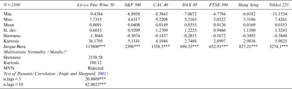
*p < .10, **p < .05, ***p < 0.01

^a Mardia's test performs multivariate skewness and kurtosis simultaneously and combines test results for multivariate normality (MVN). If both tests indicate multivariate normality, then the data follows a multivariate normality distribution at the 5% significance level.

All indexes in Table 1 yield negligible mean daily log returns. However, the mean is positive, indicating that positive changes in stock price indexes are more dominant than negative changes. Both the univariate (Jarque-Bera's test) and multivariate (Mardia's test) normality assumption are rejected.

The non-constant correlation test (Engle and Sheppard, Reference Engle and Sheppard2001) suggests that we can reject the null hypothesis in favor of a dynamic correlation model (versus static, see Table 1). This result highlights the advantage of using the DCC-GARCH model along with a more refined specification such as, for example, a time-varying copula approach.

The return data are plotted in Figure 1. As usual, in time series of financial asset returns, one can observe volatility clustering. However, this phenomenon is not present in the Live-ex-Fine Wine 50, which displays the lowest volatility (see Table 1).

Figure 1 Plots of the Daily Log-Returns of Seven Indexes

B. The Student Copula AGDCC Model

Before going into details of the Student copula AGDCC model used in this paper to model the time-varying dependence between the seven return indexes, we provide a brief overview of copula GARCH models.

A n-dimensional vector of financial time series, y_t =  (y ₁, ⋅ ⋅ ⋅ , y _p), follows a copula GARCH model if the joint cumulative distribution function is given by

(5)$$F\lpar {{\bi y}_t\;\vert \;{\bi \mu }\comma \;\;{\bi h}_t} \rpar = C\lpar {F_1\lpar {y_{1t}\;\vert \;\mu_1\comma \;h_{1t}} \rpar \comma \;\cdots \comma \;F_n\lpar {y_{nt}\;\vert \;\mu_n\comma \;h_{nt}} \rpar } \rpar \comma \;$$

where C is a n-dimensional copula, F _i the conditional distribution function of the marginal series y _it, for i = 1,  ⋅ ⋅ ⋅ , n, and y _it follows a standard univariate GARCH model:

(6)$$y_{it} = \mu _i + \sqrt {h_{it}} \;\varepsilon _{it}$$

(7)$$h_{it} = \omega _i + \alpha _i\lpar {y_{i\comma t-1}-\mu_i} \rpar ^2 + \beta _ih_{i\comma t-1}\comma \;$$

where h _it is the conditional variance of y _it given the previous information I _i,t−1 = {y _i,t−1, y _t−2, ⋅ ⋅ ⋅ }, ɛ_it are independent and identically distributed random variables with zero mean, and ω _i, α _i, β _i  > 0 and α _i + β _i < 1 to ensure positivity of h _it and covariance stationarity, respectively.

In this paper, we assume that the innovations follow a standardized skew Student distribution, ɛ_it ~ f _i(0, 1, ξ _i, υ_i ) (Fernández and Steel, Reference Fernández and Steel1998) with skew and shape parameters ξ and υ, respectively. We select this distribution because it allows for very flexible modeling of the skewness and fat tails features of the data.Footnote ² We also assume that the dependence structure between marginal series is described by a time-varying Student copula with conditional correlation R_t and constant shape parameter η. The conditional density is given by

(8)$$c_t\lpar {u_{it}\comma \;\cdots \comma \;u_{nt}\;\vert \;{\bi R}_{t\comma }\eta } \rpar = \displaystyle{{\,f_t\lpar {F_i^{{-}1} \lpar {u_{it}\vert {\eta \comma \;\cdots \comma \;F_i^{{-}1} \lpar {u_{\,pt}\vert \eta } \rpar \;} \vert \;{\bi R}_t\comma \;\eta } \rpar } \rpar } \over {\mathop \prod \nolimits_{i = 1}^n f_i\lpar {F_i^{{-}1} \lpar {u_{it}\vert \eta } \rpar \;\vert \;\eta } \rpar }}\comma \;$$

where u _it = F _it(y _it|μ _it,h _it,ξ _i,υ_i) is the Probability Integral Transformation (PIT) of each univariate series by its conditional distribution F _it estimated via the first stage GARCH processFootnote ³; $F_i^{{-}1} \lpar {u_{it}\vert \eta } \rpar$ denotes the quantile transformation of the uniform margins subject to the common shape parameter of the multivariate density; f _t( ⋅ |R_t, η) is the multivariate density of the Student distribution with conditional correlation R _t and shape parameter η; and f _i( ⋅ |η) is the univariate margins of the multivariate Student distribution with common shape parameter η. Footnote ⁴

Although there are a plethora of copula functions available in the literature (see Nelsen, Reference Nelsen2006), we select the Student copula because we suspect possible tail dependency between the marginals. Moreover, numerous previous studies suggest that the Student copula is the best choice in many cases.Footnote ⁵ Lastly, as observed by Cyr, Kwong, and Sun (Reference Cyr, Kwong and Sun2017), goodness-of-fit testing for copulas is still a relatively unresolved issue, and the complexity increases in a multivariate setting due to high dimensionality. Since we estimate here a GARCH-copula model in a d = 7-dimensional setting, and given the computational tractability of time-varying elliptic copulas in a multivariate setting (d ≥ 3), the choice of the Student-t copula is suitable.

Finally, we assume that the dynamics of R _t follows an Asymmetric Generalized Dynamic Conditional Correlations (AGDCC) model, as proposed by Cappiello, Engle, and Sheppard (Reference Cappiello, Engle and Sheppard2006). This model generalizes the DCC GARCH model of Engle (Reference Engle2002) by allowing for conditional asymmetries not only in volatilities but also in correlations. The joint density of the 2-stage estimation is defined as

(9)$$f\lpar {{\bi r}_t\vert {\bi \mu }_t\comma \;{\bi h}_t\comma \;{\bi R}_t\comma \;\eta } \rpar = c_t\lpar {u_{it}\comma \;\cdots \comma \;u_{\,pt}\vert {\bi R}_t\comma \;\eta } \rpar \mathop \prod \nolimits_{i = 1}^p \displaystyle{1 \over {\sqrt {h_{it}} }}f_{it}\lpar {\varepsilon_{it}\comma \;\upsilon_{i\comma \;\xi_i}} \rpar \comma \;$$

where the two components of the likelihood are highlighted, one due to the joint DCC copula dynamics and the other one related to the first stage univariate GARCH dynamics.

The GARCH-DCC component of the multivariate Copula-GARCH specification used in this paper is defined as a GARCH (1,1)-DCC (1,1) model. This GARCH-DCC specification is extensively used in the financial economics literature.Footnote ⁶ Also worth noting, in many cases, GARCH (1, 1) specification cannot be outperformed by more complex models (Hansen and Lunde, Reference Hansen and Lunde2005).

The conditional mean process is modeled separately for each stock return index in Table 1 in order to estimate each ARMA process independently. Selecting the “ideal” order of an ARMA model may be a cumbersome task. We select the order of the ARMA models based on the computation of the BIC and AIC information criteria for different (p, q) pairs. As a rule of thumb, when deciding between two models, the model with the lower order of differencing is preferred.

The log-likelihood function is given by the density function Equation (9). Interestingly, the log-likelihood can be easily separated into two components: the joint copula-DCC component and the univariate ARMA-GARCH component. This allows the individual ARMA-GARCH parameters and their distributional parameters to be estimated for each stock index in a first stage by maximizing the univariate ARMA-GARCH component of the LL function. Then, the copula-DCC parameters are estimated by maximizing the other component of the LL function. We use this two-stage Maximum Likelihood Estimation (MLE) approach to estimate the whole set of parameters of the Student copula AGDCC model.

C. Estimation Results of the Student Copula AGDCC Model

The Student Copula AGDCC estimation results are reported in Table 2.

• • Panel A reports the estimation results of the univariate ARMA-GARCH model for the seven indexes in the portfolio, and

• • Panel B reports the copula-DCC parameter estimation results.Footnote ⁷

Table 2 Copula-GARCH Fit

*p < .10, **p < .05, ***p < 0.01

^a ar1, ar2, and ma1 denote the AR and MA parameters, respectively. ω is the estimated value of the variance intercept parameter from the standard GARCH model of Bollerslev (Reference Bollerslev1986). Α and β denote ARCH(q) and GARCH(p), respectively. They are also called the correlation persistence parameters, with α, β ∈ (0, 1), and α + β ∈ (0, 1). ξ and ν are the skew and shape parameters, respectively, from the standardized skew Student distribution of Fernández and Steel (Reference Fernández and Steel1998).

^b a and b parameters tell whether DCC makes sense for the system of series. G denotes the asymmetry parameter of the Asymmetric Generalized DCC (AGDCC) of Cappiello, Engle, and Sheppard (Reference Cappiello, Engle and Sheppard2006). η is the shape parameter of the Student-t copula.

Panel A shows that the α, β correlation persistence parameters of the GARCH (1, 1) are never jointly non-significant, indicating that a GARCH (1, 1) is better than a constant conditional variance. The high significance of the ξ, ν-skew, and ν-shape (or tail thickness) parameters—on all indexes except the S&P 500 and FTSE 100 shape parameter—suggests that the standardized skew Student distribution of Fernández and Steel (Reference Fernández and Steel1998) is a conditional distribution consistent with the system of series.

The estimates of the ν-shape parameter of the skew Student distribution reported in Panel A are low (ranging from 4.3233 to 7.2377). It should be noted that values lower than 10 might indicate that the standardized residuals still exhibit fat-tailedness even after the volatility adjustment of stock returns through the use of GARCH modeling. However, the copula approach copes with heterogeneity in marginal distribution efficiently. Therefore, the ν-shape parameter values in Panel A are unlikely to lead to misspecification issues in the second stage of the whole likelihood maximization process (Panel B).

Lastly, we calculate the persistence parameter $\hat{P} = \mathop \sum \nolimits_{j = 1}^q \alpha _j + \mathop \sum \nolimits_{j = 1}^p \beta _j$ for the standard GARCH model (Bollerslev, Reference Bollerslev1986) to quantify the volatility clustering captured by such models. All persistence parameters in Panel A are higher than 0.9. Hence, we conclude that a DCC model is more realistic than its constant counterpart (CCC).

We proceed with a comprehensive set of fit diagnostics, including plots and various tests.Footnote ⁸ First, we assess the adequacy of the ARMA fit through a weighted Ljung-Box portmanteau test on standardized residuals. Then, we test the null hypothesis of adequately fitted ARCH process through an ARCH LM test (another weighted portmanteau test).Footnote ⁹ Lastly, to capture possible misspecification of the GARCH model, we test the presence of leverage effects (asymmetric positive and negative shocks on the conditional variance, see Glosten, Jagannathan, and Runkle, Reference Glosten, Jagannathan and Runkle1993) by using the sign bias test of Engle and Ng (Reference Engle and Ng1993).Footnote ¹⁰ Overall, the tests confirm that the model assumptions are not seriously violated: no significant misspecification, autocorrelation, or remaining ARCH effects are detected.

Regarding Panel B, the a, b DCC parameters are both non-zero parameters with high significance, indicating that DCC is superior to CCC for the system of return time series taken jointly. This is consistent with the results from the test of Engle and Sheppard (Reference Engle and Sheppard2001) of dynamic correlation (Table 1). The g asymmetry parameter of the Asymmetric Generalized DCC (AGDCC) model in Panel B is highly significant.Footnote ¹¹ This result indicates a greater response to joint bad news than to joint good news. The η shape parameter of the Student-t copula equals 15.2504. This relatively high value suggests that the tail dependency of the standardized residuals is limited, if not null. Figure 2 plots the time-varying correlations between each pair of assets generated by the GARCH-Copula model.

Figure 2 Conditional Correlations

The outputs from the time-varying GARCH-Copula-model estimation are then used in a 1-ahead rolling forecast exercise in order to produce 1-step ahead forecasts for the seven stock indexes under review. The starting values for the simulation are provided by the corresponding outputs resulting from the estimation stage.Footnote ¹² The number of simulations is set to 2,000.

A. Modified Sharpe Ratio and Peer Performance Analysis

The traditional Sharpe ratio is a risk-adjusted measure of return per unit of risk (where risk is represented by returns’ standard deviation). We instead use the modified Sharpe ratio, as proposed by Favre and Galeano (Reference Favre and Galeano2002), that is, the ratio of expected excess return over the Cornish-Fisher VaR. Indeed, the Cornish-Fisher VaR is more appropriate for return series featuring skewness and/or excess kurtosis. Descriptive statistics in Table 1 show that the seven stock indexes under review present such characteristics. In both cases—traditional or modified—the higher the Sharpe ratio, the better the combined performance of risk and return.

The modified Sharpe ratios are displayed in Panel A of Table 3, calculated based on the 1-step ahead simulated returns. The number of simulations in the bootstrap procedure is set to 2,000. The modified VaR used as an input to the modified Sharpe ratio is estimated at the 99% confidence level in order to comply with Basel III and IV requirements regarding market risk. The modified Sharpe ratio (Favre and Galeano, Reference Favre and Galeano2002; Gregoriou and Gueyie, Reference Gregoriou and Gueyie2003) is one industry standard for measuring the risk adjusted performance of portfolios. We complement the modified Sharpe ratio with the peer-performance ratios of Ardia and Boudt (Reference Ardia and Boudt2018a, Reference Ardia and Boudt2018b) displayed in Panels B and C. The former highlights significant differences between the seven mono-asset portfolios under review here, while the latter indicates the peer performance ratios expressed as a probability of equal performance (equal), outperformance (Outperf.), and underperformance (Underperf.). The portfolio's outperformance (resp. underperfomance) ratio is defined as the percentage number of peers that have a significantly lower (resp. higher) modified Sharpe ratio, after correction for luck by applying the false discovery rate approach by Storey (Reference Storey2002).

Table 3 Peer Performance Analysis

*p < .10, **p < .05, ***p < 0.01

Note: As the portfolio under review includes seven indices, the number of peers is equal to six.

In Panel A, we observe that the Liv-ex 50 displays a negative modified Sharpe ratio. This finding clearly indicates that the Liv-ex 50 is the lowest risk-adjusted performer of the indexes.

Each asset is considered as a mono-asset portfolio. In contrast, the peer performance ratios developed by Ardia and Boudt's (Reference Ardia and Boudt2018a, Reference Ardia and Boudt2018b) work with all the assets in the portfolio taken collectively. Therefore, their approach provides further insights into the modified Sharpe ratio. Ardia and Boudt classify peer performance into three categories: equal-performance, outperformance, and underperformance:

• • Equal-performance is the percentage of peer funds (or stock indexes) that perform as well as a benchmark fund (or stock index) for which the peer performance is measured.

• • Outperformance (resp. underperformance) is defined as the percentage of peer funds (or stock indexes) that underperform (resp. outperform) the benchmark fund (or stock index).Footnote ¹⁷

As noted previously, both ratios explicitly correct for the presence of false positives through the false discovery rate approach of Storey (Reference Storey2002) and control for both relative performance using pairwise tests.Footnote ¹⁸

Results from the peer performance evaluation of the seven stock indexes under review are reported in Panels B and C of Table 3.Footnote ¹⁹ The matrix in Panel B reveals that the Liv-ex 50 modified Sharpe ratio is significantly different from all other stock indexes at the 1% confidence level. Since those highly significant differences are always negative, it can be inferred that the Liv-ex 50 risk-adjusted performance is lower than that of the traditional stock indexes. Ratios in Panel C are expressed in probabilities and provide an alternative way to look at the results. Like for Panel B, the ratios in Panel C find underperformance for the Liv-ex 50. Indeed, the underperformance ratio of the Liv-ex 50 is equal to 100%, that is, the maximal possible value given the definition of the peer performance ratios. In other words, the probability of the Liv-ex 50 underperforming its six peers is equal to one; conversely, the probability of outperforming its peers is null. The FTSE 100 provides an exact counter-example.

B. M-squared for Sortino

The M-squared for Sortino or “M2 Sortino ratio” is an M-squared calculated for downside risk instead of total risk. It is defined as:

(10)$$M_S^2 = r_p + Sortino\;ratio\;\times \lpar {\sigma_{DM}-\sigma_D} \rpar \;\comma \;$$

where $M_S^2$ is the M-squared for Sortino, r _p is the annualized portfolio return, σ _DM is the benchmark downside risk, and σ _D is the portfolio annualized downside risk.

The M2 Sortino ratio (and others such as the upside potential ratio) are metrics of rank-ordering relative performance. The Sortino ratio defined in Equation (10) is an improvement over the traditional Sharpe ratio, because it uses downside semi-variance as the measure of risk (Sortino and Price, Reference Sortino and Price1994). Minimum Acceptable Return (MAR) is the key component in such return-indicators adjusted for downside risk. MAR measures risk in terms of “not meeting the investment goal.” Moreover, by considering the real risk which investors should worry about—the downside risk—all Sortino measures provide a more relevant picture of risk-adjusted performance.

Note that, since the Sortino ratio measures excess return per unit of downside risk, a higher Sortino ratio is better. The M2 Sortino is interpreted in the same way. Table 4 presents the M-squared for Sortino of the seven return distributions under review.

Table 4 The M-squared for Sortino

Choosing the MAR is a difficult task, especially when comparing disparate investment strategies while trying to answer, “Is this something I might want in my portfolio?” Some papers recommend using the risk-free rate as the MAR. We adopt a more practitioner-oriented approach and select several standardized values, thus reporting a range of scenarios.

First, we sequentially use the historical compounded (geometric) cumulative return over the whole time period (March 1, 2010 to March 30, 2018) of each of the seven stock indexes in Table 3, Panel A. The return vector of the benchmark asset used to derive the (benchmark) annualized downside risk calculated in Equation (10) is the MSCI World index. As such, MAR1 in Panel A is the MAR defined as the cumulative return of the Liv-ex 50, until MAR7 which denotes the cumulative return of the Nikkei 225. Then, in Panel B, the MSCI World index is used both as the MAR and the benchmark asset. Last, since the four stock indexes in Table 3 are European, we use the MSCI Europe index both as the MAR and the benchmark asset in Panel C.

We adopt the same sequential approach for the annualized portfolio return, denoted as r _p in Equation (10). As a result, each of the seven stock indexes serves as a mono-asset portfolio. To illustrate, when using the cumulative return of S&P 500 as the MAR (i.e., MAR2 equals 1.1636 in Panel A), the resulting M2 Sortino of the annualized S&P 500 portfolio return is equal to 0.1689. Similarly, when using the cumulative return of Nikkei 225 (i.e., MAR7 equals 0.7512), the resulting M2 Sortino of the annualized Nikkei portfolio return equals 0.0882.

As we can see from Panel A, the Liv-ex 50 M2 Sortino is negative for all MAR (1 to 7)—confirming previous findings (i.e., Table 3 modified Sharpe ratio and peer performance). The Liv-ex 50 may not be a good portfolio addition for the investor looking to optimize his returns adjusted for downside risk performance. Unsurprisingly, no annualized mono-asset portfolio return outperforms the MSCI World index (Panel B).

C. VaR and ES

In Table 5, $VaR_\alpha \lpar {0 \lt \alpha \lt 1} \rpar$ is defined as

(11)$${\rm {\opf P}}\lpar {L \le -VaR_\alpha } \rpar = \alpha \comma \;$$

where the profit and loss random variable L is defined from d equal-weighted returns and the random vector of returns r = (r ₁, ⋅ ⋅ ⋅ , r _d) as

$$L = \mathop \sum \nolimits_{\,j = 1}^d r_i/d.$$

Table 5 VaR and ES

Table (5) reports VaR and ES estimates, calculated based on the 1-step ahead simulated returns. The number of simulations in the bootstrap procedure is set to 2,000, thus generating 2,000 1-step ahead simulated returns. mVaR99% and mES99% in Panel A and B denote the modified Cornish-Fisher measures of VaR and ES, respectively. Pf _mVaR99% and Pf _mES99% stand for the portfolio VaR and ES. The component VaR and ES indicators, Conp_mVaR and Conp_mES, measure the contribution to the VaR and ES portfolio. The component value for each stock index in the portfolio must sum to the portfolio VaR and ES (values are rounded off to the nearest five decimals). Comp_mVaR(%) and Comp_mES(%) are the percent contribution to the portfolio VaR and ES. The percentage contributions to the portfolio VaR and ES must add up to 100% (values are rounded off to the nearest two decimals). We complement the VaR and ES estimates with the Diversification Measures in Panel C, computed according to Choueifaty and Coignard (Reference Choueifaty and Coignard2008). Opt. Weights (%) denotes the optimal weights (expressed as percentages) for the Most Diversified Portfolio solution. Div. Ratio and Con. Ratio stand for the Diversification ratio and the Concentration ratio, respectively. Vwac indicates the Volatility weighted average correlation. By construction, the diversification ratio of any long-only portfolio is strictly greater than 1 (except when the portfolio is equivalent to a mono-asset portfolio, in which case the diversification ratio equals 1). A higher diversification ratio indicates a higher-diversified portfolio.

Panel A reports the VaR results. The Liv-ex 50 displays the highest modified VaR at the 99% confidence level (mVaR_99% in Panel A). Unsurprisingly, all individual VaRs are higher than the entire portfolio VaR (Pf_mVaR_99% in Panel A).

The component VaR is the risk contribution of each asset to the risk of the entire portfolio VaR. Component VaRs add up to the value of the whole portfolio VaR. In our analysis, the component VaR (Comp_mVaR in Panel A) indicates that the Liv-ex 50 is the “strongest diversifier” within the seven-asset portfolio. In other words, it is expected that removing the Liv-ex 50 would increase the portfolio VaR. With the lowest component VaR, the Liv-ex 50 contributes only 1.61% of the portfolio total risk (Comp_mVaR(%) in Panel A).

ES is defined as the mean expected loss when the loss exceeds the VaR. That is,

(12)$$ES_\alpha = {-}E\lpar {L\vert L \le \;-VaR_\alpha } \rpar .$$

To be consistent with the VaR calculation, we use a modified ES. The results from Table 5 (Panel B) confirm the conclusions derived earlier from the analysis of VaR. Indeed, the Liv-ex 50 reports the highest modified ES (mES_99%) and is the “largest diversifier.” The Liv-ex 50 is the smallest contributor to total portfolio risk (Comp_mES), contributing only 1.37% to the portfolio ES (Comp_mES(%)).

Panel C of Table 5 complements the VaR and ES analysis with diversification measures proposed by Choueifaty and Coignard (Reference Choueifaty and Coignard2008). The analysis checks whether our previous conclusions about diversification benefits hold true when diversification measures are used.

We consider the following three diversification measures: (1) the diversification ratio denoted as Div. Ratio in Panel C, (2) the concentration ratio (Con. Ratio), and (3) the volatility weighted average correlation Vwac.Footnote ²⁰

The diversification ratio of a portfolio is the weighted average of the assets’ volatilities divided by the portfolio volatility, defined as

(13)$$DR\lpar \omega \rpar = \displaystyle{{\mathop \sum \nolimits_{i = 1}^N \omega _i\sigma _i} \over {\sqrt {\omega ^{\prime}\sum \omega } }}\comma \;$$

where N is the number of assets in portfolio, and Σ the variance-covariance matrix of asset returns.

The concentration ratio is defined as

(14)$$CR = \displaystyle{{\mathop \sum \nolimits_{i = 1}^N {\lpar {\omega_i} \rpar }^2} \over {{\left({\mathop \sum \nolimits_{i = 1}^N \omega_i\sigma_i} \right)}^2}}.$$

The volatility-weighted average correlation of the assets is defined as

(15)$$\rho \lpar \omega \rpar = \displaystyle{{\mathop \sum \nolimits_{i \gt j}^N \lpar {\omega_i\sigma_i\omega_j\sigma_j} \rpar \rho _{ij}} \over {\mathop \sum \nolimits_{i \gt j}^N \lpar {\omega_i\sigma_i\omega_j\omega_j} \rpar }}.$$

We first calculate these three metrics for an equally-weighted portfolio. We then duplicate the analysis with the Most-Diversified Portfolio (MDP) derived from the optimal weights (expressed in percentages in Panel C).Footnote ²¹

As we can see in Panel C, the MDP diversification ratio (Div. Ratio) is, unsurprisingly, higher than the equally-weighted portfolio's Div. Ratio. This holds true when looking at both the concentration ratio (Con. Ratio) and the volatility weighted average correlation (Vwac).

The weights of the MDP, Opt. Weights (%), provide more interesting results. They confirm that the Liv-ex 50 is the “strongest” or best diversifier (with the highest Opt. Weights at 43.58%). In other words, an investor looking to reduce risk through diversification should weight the Liv-ex 50 up to around 44%, thus obtaining maximum diversification gains.Footnote ²² This result confirms and refines conclusions drawn from the analysis of VaR and ES (Panels A and B of Table 5). In sum, the Liv-ex 50 is a very powerful risk-reduction alternative asset and might be a pillar of any portfolio diversification strategy.

D. Beta Co-Moments

The higher moments and co-moments of a return distribution can be analyzed to identify diversification potential. They are the “beta” or “systematic” moments. Higher moment betas are used to estimate the risk impact of adding an asset to a portfolio. Ranaldo and Favre (Reference Ranaldo and Favre2005) define co-skewness and co-kurtosis as the skewness and kurtosis of a given asset analyzed with reference to the skewness and kurtosis of a benchmark.

Table 6 reports the multivariate moments or co-moments (Panel A) and their beta or systematic counterparts (Panel B) for seven portfolios of six assets each {Pf.1, …, Pf.7}. These portfolios are then used in co-moments and beta co-moments analyses as the reference or benchmark portfolio. co-skewness and co-kurtosis define the skewness and kurtosis of a given asset analyzed with the skewness and kurtosis of each of the seven benchmark portfolio {Pf.1, …, Pf.7}. Similarly, beta co-skewness and beta co-kurtosis test for systematic skewness and kurtosis between a given asset and the benchmark portfolio under review. A negative (resp. positive) co-skewness means that a given asset tends to have an asymmetric tail extending towards more negative (resp. positive) returns with respect to the distribution of the benchmark portfolio. co-kurtosis measures the likelihood that extreme returns jointly occur in a given asset and in the benchmark portfolio. A positive (resp. negative) co-kurtosis means that a given asset is adding (resp. subtracting) kurtosis to the benchmark portfolio. Hence, the insertion (resp. exclusion) of this asset into the benchmark portfolio will strengthen (resp. weaken) the likelihood of extreme returns.

Table 6 Beta Co-Moments

Notes: Positive values for skewness and excess kurtosis indicate positive skewness and leptokurtosis (long tails), respectively, whereas negative values for skewness and excess kurtosis indicate negative skewness and platykurtosis (short tails). The number of simulations in the bootstrap procedure is set to 2000.

*Each equally weighted benchmark portfolio under review includes six assets:

Pf.1 = {S&P, CAC, DAX, FTSE, Hang Seng, Nikkei}

Pf.2 = {Liv-ex 50, CAC, DAX, FTSE, Hang Seng, Nikkei}

Pf.3 = {Liv-ex 50, S&P, DAX, FTSE, Hang Seng, Nikkei}

Pf.4 = {Liv-ex 50, S&P, CAC, FTSE, Hang Seng, Nikkei}

Pf.5 = {Liv-ex 50, S&P, CAC, DAX, Hang Seng, Nikkei}

Pf.6 = {Liv-ex 50, S&P, CAC, DAX, FTSE, Nikkei}

Pf.7 = {Liv-ex 50, S&P, CAC, DAX, FTSE, Hang Seng}

Theory suggests that ceteris paribus, rational investors dislike negative co-skewness and positive co-kurtosis. For instance, Scott and Horvath (Reference Scott and Horvath1980) show that an investor with a positive preference for positive skewness—and displaying consistent risk aversion—exhibit a negative preference for kurtosis. Harvey and Siddique (Reference Harvey and Siddique2000) find that co-skewness is priced in equity markets.Footnote ²³ Dittmar (Reference Dittmar2002) finds that co-kurtosis is priced in equity markets: investors require to be compensated for the additional risk undertaken when a portfolio exhibits negative co-skewness and positive co-kurtosis. In contrast, investors are willing to accept a lower return in the opposite situation. In short, a positive co-skewness and a negative co-kurtosis reduce the opportunities for seeking risk compensation.

The choice of a benchmark is critical since results may be sensitive to that choice. To provide a four-moment extension to the two-moment CAPM, Christie-David and Chaudhry (Reference Christie-David and Chaudhry2001) use nine different market proxies (weighted to non-weighted future indexes). They also employ an all-equity index—the S&P 500 cash index—as a market proxy. They find that their results are robust to the market proxy used, thus providing some freedom to select the benchmark portfolio.

In Table 6, we consider seven equally-weighted benchmark portfolios denoted as {Pf.1, …, Pf.7}. Each is composed of six assets selected among the seven indexes under review in this paper (the Liv-ex 50 and the six stock indexes). The co-moments (Panel A) and beta co-moments (Panel B) in Table 6 are computed between a single asset and a benchmark portfolio. The single asset i (i = 1, …, 7) involves in the calculation of the co-moments and beta co-moments is not included in the benchmark portfolio j (j = 1, … 7).

As an example, to compute the co-moments and beta co-moments between the Liv-ex 50 and the first benchmark portfolio in Table 6, denoted as Pf1, we exclude the Liv-ex 50 from this portfolio. The aim is to isolate the individual effect of a single asset when it is adding to a benchmark portfolio.

For instance, if the Liv-ex 50 is added to the first benchmark portfolio Pf1 = {S&P, CAC, DAX, FTSE, Hang Seng, Nikkei}, what about the co-moments and the beta co-moments of this portfolio? Are they going to move upward or downward? Answering this question is relevant from both a risk and portfolio management perspectives.

The results in Table 6 Panel B show a negative beta co-variance between the Liv-ex 50 and the benchmark portfolio Pf1. In other words, adding the Liv-ex 50 to this portfolio will reduce its volatility.

Moreover, the Liv-ex 50 generates the highest diversification gain; it is the only one displaying a negative co-variance. This result is really attractive for a risk-averse investor. Indeed, the lower the beta, the higher the diversification effect in terms of volatility, risk of asymmetry (co-skewness), and extreme events (co-kurtosis).

Positive beta co-skewness means that the asset under review (or, equivalently, the mono-asset portfolio) tends to have an asymmetric tail extending towards more positive returns with respect to the distribution of the benchmark portfolio returns. A rational investor prefers positive co-skewness due to the lower downside risk. The Liv-ex 50 displays the lowest positive beta co-skewness. As aforementioned, the lower the beta, the higher the diversification effect in terms of the risk of asymmetry.

A positive co-kurtosis (such as that displayed in portfolios Pf.2, …, Pf.7) adds kurtosis to the portfolio benchmark. To illustrate, adding S&P 500 in Pf.2 (built exclusive of S&P 500) increases the kurtosis of the resulting Pf.2 benchmark portfolio. In other words, adding S&P 500 increases the likelihood of extreme returns. In contrast, the Liv-ex 50 is the only asset reporting a negative co-kurtosis with reference to its Pf.1 benchmark portfolio (see Table 6 Panel B). This indicates that thanks to its positive beta co-kurtosis, the Liv-ex 50 is the only asset able to reduce the probability of extreme co-variations with its benchmark portfolio.

To conclude, given its negative beta co-variance, low beta co-skewness and negative co-kurtosis (with reference to its benchmark portfolio), the Liv-ex 50 displays the highest diversification benefits in terms of volatility, asymmetry, and extreme events.