1 Introduction
Over the years, the motion of air bubbles in complex fluids with yield stress has drawn the attention of many research groups, due to both the fundamental nature of this problem and the wide range of scientific, engineering and even geophysical applications. Characteristic examples of such applications include (i) prevention of bubble formation and expansion in adhesives (Foteinopoulou et al. Reference Foteinopoulou, Mavrantzas, Dimakopoulos and Tsamopoulos2006; Papaioannou et al. Reference Papaioannou, Giannousakis, Dimakopoulos and Tsamopoulos2014) and bubble removal from structural materials (e.g. cement) because their presence may significantly degrade the mechanical properties, (ii) mobilization of bubbles containing oxygen to accelerate waste treatment and fermentation processes (Blanch & Bhavaraju Reference Blanch and Bhavaraju1976), (iii) control of air bubbles in foods to improve their texture (e.g. aerated chocolate, ketchup, mayonnaise) (Campbell Reference Campbell2016), or various cosmetic products to increase their volume (e.g. hand creams, hair gels, toothpaste), (iv) inhibition of large bubble formation in drilling mud, which may cause dangerous explosions, delay production and potentially inflict a huge burden on ecosystems and the finances of oil-drilling companies (Johnson & White Reference Johnson and White1991; BP report 2010) and (v) the role of bubble dynamics in volcanic activities, e.g. eruptions, earthquakes or inflation of volcanoes (Ichihara & Nishimura Reference Ichihara, Nishimura and Meyers2011; Tran, Rudolph & Manga Reference Tran, Rudolph and Manga2015). In all these applications we are often concerned with the mobility and dynamics of gas bubbles under different conditions, and the purpose of this paper is to examine how these are affected in the presence of an acoustic field.
The motion of a bubble through a viscoplastic material exhibits some interesting aspects, which cannot be directly deduced from the corresponding laws for Newtonian liquids. It is well known, for example, that bubbles may become entrapped indefinitely in a viscoplastic material when their buoyancy is sufficiently small compared to the yield stress, owing to their inability to break the weak physical bonds in the material. This was first demonstrated in the experiments performed by Astarita & Apuzzo (Reference Astarita and Apuzzo1965) who reported bubble shapes and velocities in Carbopol solutions and slightly or highly elastic liquids. Their experiments revealed that curves of bubble velocity versus bubble volume had an abrupt change in slope at a critical value of bubble volume that depended on the concentration of Carbopol in the solution. Terasaka & Tsuge (Reference Terasaka and Tsuge2001) studied the formation of bubbles at a nozzle in yield-stress fluids (xanthan gum and Carbopol) and provided an approximate model for bubble growth. A model, based on variational inequalities, to obtain the critical conditions for bubble entrapment in viscoplastic fluids was proposed by Dubash & Frigaard (Reference Dubash and Frigaard2004, Reference Dubash and Frigaard2007); these estimations, however, were characterized as conservative, in the sense that they provide a sufficient but not necessary condition. They compared their predictions with experiments and found that surface tension affects significantly the bubble stopping conditions. Their experiments also revealed that the bubbles had a rounded shape on their front, but terminated downstream in a cusp. These findings were confirmed by Sikorski, Tabureau & de Bruyn (Reference Sikorski, Tabureau and de Bruyn2009) and Mougin, Magnin & Piau (Reference Mougin, Magnin and Piau2012) who conducted detailed and careful experiments to investigate the shape, trajectory and dynamics of an air bubble in Carbopol solutions of various concentrations.
An early attempt to address this problem theoretically was made by Bhavaraju, Mashelkar & Blanch (Reference Bhavaraju, Mashelkar and Blanch1978) who considered a spherical air bubble and performed a regular perturbation analysis in the singular limit of small yield stress. A detailed numerical study of the steady rise of a deformable bubble was performed much later by Tsamopoulos et al. (Reference Tsamopoulos, Dimakopoulos, Chatzidai, Karapetsas and Pavlidis2008), employing a regularized model (Papanastasiou Reference Papanastasiou1987) to account for viscoplastic effects and fully taking into account the effects of inertia, surface tension and gravity. Their calculations provided a more accurate evaluation of the conditions for bubble entrapment than the conservative estimate provided by Dubash & Frigaard (Reference Dubash and Frigaard2004, Reference Dubash and Frigaard2007). A more accurate estimation of the stopping conditions was made by Dimakopoulos, Pavlidis & Tsamopoulos (Reference Dimakopoulos, Pavlidis and Tsamopoulos2013), Dimakopoulos et al. (Reference Dimakopoulos, Makrigiorgos, Georgiou and Tsamopoulos2018) who employed the augmented Lagrangian method to account for the discontinuous behaviour of the constitutive model. Tripathi et al. (Reference Tripathi, Sahu, Karapetsas and Matar2015) showed through time-dependent simulations that rise dynamics may become complex in the case of highly deformable bubbles, punctuated by periods of rapid acceleration which separate stages of quasi-steady motion. Finally, the interaction of multiple bubbles or droplets in a yield-stress fluid has been examined by Potapov et al. (Reference Potapov, Spivak, Lavrenteva and Nir2006), Singh & Denn (Reference Singh and Denn2008) and Islam, Ganesan & Cheng (Reference Islam, Ganesan and Cheng2015). It is noteworthy that inverted teardrop shapes, observed in experiments, were not reported in any of these theoretical works probably because the effect of fluid elasticity was ignored. The importance, though, of even small amounts of fluid elasticity, encountered in real yield-stress fluids such as Carbopol, has been discussed in detail in Fraggedakis, Dimakopoulos & Tsamopoulos (Reference Fraggedakis, Dimakopoulos and Tsamopoulos2016a ,Reference Fraggedakis, Dimakopoulos and Tsamopoulos b ) and its effect on bubble shapes was confirmed very recently by experiments performed by Lopez, Naccache & de Souza Mendes (Reference Lopez, Naccache and de Souza Mendes2018).
It has been suggested that an increase in the mobility of a bubble could be achieved by applying an oscillatory pressure field or vibrations (Stein & Buggisch Reference Stein and Buggisch2000; Iwata et al. Reference Iwata, Yamada, Takashima and Mori2008). The presence of an acoustic field causes volume oscillation of the bubble, due to its compressibility, modifying the stress in the liquid surrounding the bubble and thus allowing it to overcome the yield stress of the material. In fact, this is a well-established practice in the construction business where vibrators are often used to de-aerate and consolidate concrete (ACI Committee 1993, 1996). Besides engineering applications, this mechanism is also very relevant to geophysical phenomena, where pressure perturbations, e.g. caused by passing seismic waves from a near or distant source, may affect the mobility of bubbles entrained in magmas (Ichihara & Nishimura Reference Ichihara, Nishimura and Meyers2011).
The response of bubbles to pressure forces driven by sound waves has been studied extensively in the case of Newtonian fluids; extensive reviews can be found in Plesset & Prosperetti (Reference Plesset and Prosperetti1977), Feng & Leal (Reference Feng and Leal1997) and Lauterborn & Kurz (Reference Lauterborn and Kurz2010). It has been established that under the action of an acoustic pressure wave, besides radial oscillation, a bubble is also forced into a translational motion relative to the surrounding fluid due to the action of the primary ‘Bjerknes’ force (see Brennen Reference Brennen2014). This interaction of acoustic and hydrodynamic forces can give rise to complex flow dynamics (e.g. Pelekasis & Tsamopoulos Reference Pelekasis and Tsamopoulos1993a ,Reference Pelekasis and Tsamopoulos b ; Rensen et al. Reference Rensen, Bosman, Magnaudet, Ohl, Prosperetti, Togel, Verluis and Lohse2001; Chatzidai, Dimakopoulos & Tsamopoulos Reference Chatzidai, Dimakopoulos and Tsamopoulos2011). In order to account for this complex behaviour, theoreticians have developed models of varying complexity assuming either bubbles with spherical shape undergoing volume oscillations (Doinikov Reference Doinikov2002; Reddy & Szeri Reference Reddy and Szeri2002a ; Krefting et al. Reference Krefting, Toilliez, Szeri, Mettin and Lauterborn2006) or deformable bubbles that may also exhibit shape oscillations (Reddy & Szeri Reference Reddy and Szeri2002b ; Doinikov Reference Doinikov2004; Shaw Reference Shaw2006); in these works, the effect of buoyancy was typically neglected.
Another degree of complexity is introduced when gravitational effects are important since the dynamics of the bubble will also be affected by its rising motion due to buoyancy. A reduced-order model was derived by Gordillo et al. (Reference Gordillo, Lalanne, Risso, Legendre and Tanguy2012) to investigate the coupling between bubble acceleration and deformation, considering a bubble with constant volume and small perturbations to its spherical shape. The motion of a spherical pulsating bubble under gravity was investigated by Chakraborty & Tuteja (Reference Chakraborty and Tuteja1993) and later by Tuteja et al. (Reference Tuteja, Khattar, Chakraborty and Bansal2010) using the Lagrangian formalism to derive a fully two-way coupled model. Ricciardi & De Bernardis (Reference Ricciardi and De Bernardis2016) recently used a similar methodology to investigate the acoustic emission of a pulsating bubble in an inviscid liquid. Numerical simulations, solving the full Navier–Stokes equations and fully accounting for the deformability of the bubble, were also employed by Yang, Prosperetti & Takagi (Reference Yang, Prosperetti and Takagi2003) and Lalanne, Tanguy & Risso (Reference Lalanne, Tanguy and Risso2013) to investigate the interaction of shape oscillations and rising motion; a simpler model based on force balances to investigate the same problem has been developed by de Vries, Luther & Lohse (Reference de Vries, Luther and Lohse2002). Numerical simulations were also used by Romero, Torczynski & von Winckel (Reference Romero, Torczynski and von Winckel2014) to evaluate the terminal velocity in a vertically vibrated liquid which produces oscillations in both pressure and gravitational fields.
In the case of non-Newtonian fluids, interest has focused mainly on liquids that exhibit either a generalized viscous behaviour or viscoelastic effects (see Brujan Reference Brujan2009 and Cunha & Albernaz Reference Cunha and Albernaz2013). In the latter case, the most significant effects arise due to the response of viscoelastic liquids in an extensional flow such as that generated around a bubble during its growth and collapse phase. As reported in Iwata et al. (Reference Iwata, Yamada, Takashima and Mori2008), the effect of elasticity becomes more obvious during the compression phase where the cusp shape arises. The case of viscoplastic materials, though, has received considerably less attention with two notable exceptions. Chan & Yang (Reference Chan and Yang1969) considered a spherical gas bubble ignoring the effect of buoyancy and derived a generalized Rayleigh–Plesset equation, accounting for the yield stress of the material and investigated the dynamics of a bubble subject to harmonic pressure fluctuations close to the natural frequency of the system. Stein & Buggisch (Reference Stein and Buggisch2000), as mentioned above, were interested in the mobilization of bubbles by setting an oscillating external pressure and provided simplified analytical solutions along with some experimental data; the latter suggested that larger bubbles tend to rise faster than smaller bubbles at similar amplitudes.
The goal of our work is to investigate in detail the dynamics of a bubble inside a viscoplastic medium that is subjected to an acoustic pressure field. Our approach fully takes into account the effects of inertia, surface tension and gravity. First, we develop a reduced-order model assuming that the bubble has a spherical shape and then we proceed with numerical simulations of a deformable bubble, solving the momentum conservation equation assuming axial symmetry. For the purposes of the present study, the effects of elasticity will be ignored, and we will focus only on the role of yield stress. To this end, we employ the discontinuous Bingham constitutive equation for the reduced-order model and the regularized Papanastasiou model for the axisymmetric simulations. As has been shown by Tsamopoulos et al. (Reference Tsamopoulos, Dimakopoulos, Chatzidai, Karapetsas and Pavlidis2008), the latter model, when used with caution, provides a good understanding of the qualitative and in many cases quantitative characteristics of the flow. A thorough parametric study will be presented to investigate the dynamics of the system and determine the conditions under which acoustic excitation may enhance bubble mobility.
This paper is organized as follows. In § 2 the physical problem is described. A sphero-symmetric reduced-order model is derived in § 3, while a more detailed model assuming axial symmetry and its numerical implementation are discussed in § 4. A discussion of the results from our numerical simulations for both models and a thorough parametric analysis are presented in § 5. Conclusions are drawn in § 6.
2 Physical problem
We examine the dynamics of an axisymmetric gas bubble rising through a viscoplastic medium which is subjected to acoustic excitation (depicted schematically in figure 1). The viscoplastic liquid is considered to be incompressible with density,
 $\unicode[STIX]{x1D70C}$
, exhibiting a constant yield stress,
$\unicode[STIX]{x1D70C}$
, exhibiting a constant yield stress,
 $\unicode[STIX]{x1D70F}_{y}$
, and upon yielding a constant dynamic viscosity,
$\unicode[STIX]{x1D70F}_{y}$
, and upon yielding a constant dynamic viscosity,
 $\unicode[STIX]{x1D707}$
. The density and viscosity of the gas inside the bubble are assumed to be much smaller than those of the liquid, so that the gas is considered to be inertialess and inviscid. Finally, a constant interfacial tension of the liquid–gas interface,
$\unicode[STIX]{x1D707}$
. The density and viscosity of the gas inside the bubble are assumed to be much smaller than those of the liquid, so that the gas is considered to be inertialess and inviscid. Finally, a constant interfacial tension of the liquid–gas interface,
 $\unicode[STIX]{x1D6FE}$
, is assumed.
$\unicode[STIX]{x1D6FE}$
, is assumed.

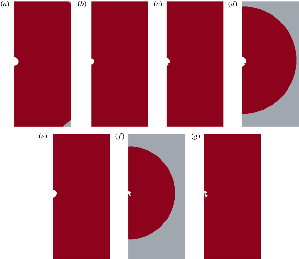
Figure 1. Schematic of a pulsating bubble rising in an unbounded viscoplastic liquid under the effect of an acoustic pressure field and the coordinate system in a reference frame that follows the bubble motion. (a) Model assuming sphero-symmetric bubble oscillations and (b) axisymmetric model. Here
 $\unicode[STIX]{x1D6FA}$
denotes the volume of the surrounding viscoplastic material and
$\unicode[STIX]{x1D6FA}$
denotes the volume of the surrounding viscoplastic material and
 $S_{1}$
and
$S_{1}$
and
 $S_{2}$
denote the surface of the liquid–gas interface (at
$S_{2}$
denote the surface of the liquid–gas interface (at
 $r=R$
) and the outflow boundary at
$r=R$
) and the outflow boundary at
 $r=R_{\infty }$
, respectively.
$r=R_{\infty }$
, respectively.
Initially, the gas bubble is at equilibrium with the surrounding material and depending on the yield stress of the viscoplastic liquid the bubble may either be entrapped in the liquid or rise with a constant velocity under the effect of buoyancy. Thus, we assume that, under these equilibrium conditions, the bubble has an initial pressure
 $P_{go}$
, volume
$P_{go}$
, volume
 $V_{o}$
with a nominal radius
$V_{o}$
with a nominal radius
 $R_{o}=(3V_{o}/4\unicode[STIX]{x03C0})^{1/3}$
and may rise in the liquid with a velocity
$R_{o}=(3V_{o}/4\unicode[STIX]{x03C0})^{1/3}$
and may rise in the liquid with a velocity
 $U_{o}$
, while the pressure at far field is given by
$U_{o}$
, while the pressure at far field is given by
 $P_{o}(z)=P_{r}-\unicode[STIX]{x1D70C}gz$
;
$P_{o}(z)=P_{r}-\unicode[STIX]{x1D70C}gz$
;
 $g$
denotes the gravitational acceleration. Parameter
$g$
denotes the gravitational acceleration. Parameter
 $P_{r}$
denotes the reference pressure which is chosen to be the equilibrium pressure in the liquid at the same level as the initial position of the bubble centre of mass (i.e. at
$P_{r}$
denotes the reference pressure which is chosen to be the equilibrium pressure in the liquid at the same level as the initial position of the bubble centre of mass (i.e. at
 $z(t=0)=0$
). At time
$z(t=0)=0$
). At time
 $t=0$
, a single-frequency acoustic excitation is applied by imposing the following sinusoidal variation of the liquid pressure far from the bubble:
$t=0$
, a single-frequency acoustic excitation is applied by imposing the following sinusoidal variation of the liquid pressure far from the bubble:
 $$\begin{eqnarray}P_{\infty }(z,t)=P_{r}[1+a\sin (ft)]-\unicode[STIX]{x1D70C}gz,\end{eqnarray}$$
where
 $a$
and
$a$
and
 $f$
are the amplitude and angular frequency of the imposed pressure oscillation. We assume that, under the action of the acoustic pressure field, the gas inside the bubble undergoes a polytropic process and the pressure of the gas inside the bubble depends on the bubble volume according to the following law:
$f$
are the amplitude and angular frequency of the imposed pressure oscillation. We assume that, under the action of the acoustic pressure field, the gas inside the bubble undergoes a polytropic process and the pressure of the gas inside the bubble depends on the bubble volume according to the following law:
 $$\begin{eqnarray}P_{g}(t)=P_{go}[V_{o}/V(t)]^{k},\end{eqnarray}$$
where
 $P_{g}(t)$
and
$P_{g}(t)$
and
 $V(t)$
are the pressure of the gas in the bubble and the volume of the bubble, respectively, at a certain time instant and
$V(t)$
are the pressure of the gas in the bubble and the volume of the bubble, respectively, at a certain time instant and
 $k$
denotes the polytropic constant, with
$k$
denotes the polytropic constant, with
 $1\leqslant k\leqslant 1.4$
. Hereafter, we will restrict ourselves to the case of a bubble undergoing an adiabatic process and thus consider the case of
$1\leqslant k\leqslant 1.4$
. Hereafter, we will restrict ourselves to the case of a bubble undergoing an adiabatic process and thus consider the case of
 $k=1.4$
. Here
$k=1.4$
. Here
 $P_{go}=P_{r}+2\unicode[STIX]{x1D6FE}/R_{o}$
denotes the gas pressure in the bubble at equilibrium.
$P_{go}=P_{r}+2\unicode[STIX]{x1D6FE}/R_{o}$
denotes the gas pressure in the bubble at equilibrium.
3 One-dimensional sphero-symmetric model
In this part of our work, we will derive a simple one-dimensional model by assuming spherical symmetry of the bubble. The simplest way to model a spherical bubble which oscillates and translates simultaneously would be to decouple the two motions, i.e. to solve the radial equations by using a Rayleigh–Plesset type of equation and then use the variation of the bubble radius with time as an input for the translation equation which can be obtained by applying Newton’s second law. Such an approach has been used by Watanabe & Kukita (Reference Watanabe and Kukita1993) and Matula (Reference Matula2003), but is limited by the fact that the feedback of the translational motion on the radial oscillation is completely ignored.
An alternative and more rigorous approach has been suggested by Chakraborty & Tuteja (Reference Chakraborty and Tuteja1993) and was later also used by Tuteja et al. (Reference Tuteja, Khattar, Chakraborty and Bansal2010) and Ricciardi & De Bernardis (Reference Ricciardi and De Bernardis2016) to investigate the motion of a spherically pulsating gas bubble under gravity for the case of either an inviscid or a viscous Newtonian fluid. According to this method, the radial and translational motions are fully coupled, and the relevant equations are derived simultaneously by using the Lagrangian formalism. A similar approach has been used by Doinikov (Reference Doinikov2002) to investigate the coupled dynamics of a bubble moving under the effect of pressure gradient due to a forcing acoustic field. Here, we will employ the same methodology based on the Lagrangian formalism to derive the coupled set of equations for the case of a pulsating bubble moving under the effect of buoyancy inside a viscoplastic liquid.
The flow in the viscoplastic material is governed by the momentum and mass conservation equations
 $$\begin{eqnarray}\displaystyle & \displaystyle \unicode[STIX]{x1D70C}\left(\frac{\unicode[STIX]{x2202}\boldsymbol{u}}{\unicode[STIX]{x2202}t}+\boldsymbol{u}\boldsymbol{\cdot }\unicode[STIX]{x1D735}\boldsymbol{u}\right)+g\boldsymbol{e}_{z}+\unicode[STIX]{x1D735}P=\unicode[STIX]{x1D735}\boldsymbol{\cdot }\unicode[STIX]{x1D64F}, & \displaystyle\end{eqnarray}$$
 $$\begin{eqnarray}\displaystyle & \displaystyle \unicode[STIX]{x1D735}\boldsymbol{\cdot }\boldsymbol{u}=0. & \displaystyle\end{eqnarray}$$
For the purposes of the present simplified approach, we will consider the Bingham constitutive equation to account for the viscoplasticity of the surrounding material:
 $$\begin{eqnarray}\displaystyle & \displaystyle \unicode[STIX]{x1D64F}=\left(\unicode[STIX]{x1D707}+\frac{\unicode[STIX]{x1D70F}_{y}}{\Vert \unicode[STIX]{x1D71E}\Vert }\right)\unicode[STIX]{x1D71E}\quad \text{for }\unicode[STIX]{x1D70F}>\unicode[STIX]{x1D70F}_{y}, & \displaystyle\end{eqnarray}$$
 $$\begin{eqnarray}\displaystyle & \displaystyle \Vert \unicode[STIX]{x1D71E}\Vert =\mathbf{0}\quad \text{for }\unicode[STIX]{x1D70F}<\unicode[STIX]{x1D70F}_{y}, & \displaystyle\end{eqnarray}$$
where
 $\unicode[STIX]{x1D71E}$
and
$\unicode[STIX]{x1D71E}$
and
 $\Vert \unicode[STIX]{x1D71E}\Vert$
denote the rate of strain tensor,
$\Vert \unicode[STIX]{x1D71E}\Vert$
denote the rate of strain tensor,
 $\unicode[STIX]{x1D71E}=\unicode[STIX]{x1D735}\boldsymbol{u}+\unicode[STIX]{x1D735}\boldsymbol{u}^{\text{T}}$
, and its second invariant,
$\unicode[STIX]{x1D71E}=\unicode[STIX]{x1D735}\boldsymbol{u}+\unicode[STIX]{x1D735}\boldsymbol{u}^{\text{T}}$
, and its second invariant,
 $\Vert \unicode[STIX]{x1D71E}\Vert =\sqrt{(\unicode[STIX]{x1D71E}\boldsymbol{ : }\unicode[STIX]{x1D71E})/2}$
, respectively.
$\Vert \unicode[STIX]{x1D71E}\Vert =\sqrt{(\unicode[STIX]{x1D71E}\boldsymbol{ : }\unicode[STIX]{x1D71E})/2}$
, respectively.
We assume that the flow around the spherical pulsating bubble remains irrotational except for a very small region near the liquid–gas interface. Under this assumption, it is possible to introduce a velocity potential such that
 $\boldsymbol{u}=-\unicode[STIX]{x1D735}\unicode[STIX]{x1D711}$
. This assumption is typically used for inviscid fluids, but can be extremely useful even for the case of viscous fluids. As will be shown below, the model that will be derived using this assumption provides a prediction of the critical Bn for bubble entrapment, in the absence of an acoustic field, which is remarkably close to the exact value. For an extended discussion of the plausibility of the vorticity-free approximation for viscous liquids, we refer the reader to Joseph & Wang (Reference Joseph and Wang2004) and Joseph (Reference Joseph2006).
$\boldsymbol{u}=-\unicode[STIX]{x1D735}\unicode[STIX]{x1D711}$
. This assumption is typically used for inviscid fluids, but can be extremely useful even for the case of viscous fluids. As will be shown below, the model that will be derived using this assumption provides a prediction of the critical Bn for bubble entrapment, in the absence of an acoustic field, which is remarkably close to the exact value. For an extended discussion of the plausibility of the vorticity-free approximation for viscous liquids, we refer the reader to Joseph & Wang (Reference Joseph and Wang2004) and Joseph (Reference Joseph2006).
Assuming a spherical polar system of coordinates
 $(r,\unicode[STIX]{x1D703})$
with origin at the centre of the bubble (see figure 1
a) and the axis of symmetry aligned with the bubble velocity
$(r,\unicode[STIX]{x1D703})$
with origin at the centre of the bubble (see figure 1
a) and the axis of symmetry aligned with the bubble velocity
 $U$
, the velocity potential function is given by
$U$
, the velocity potential function is given by
 $$\begin{eqnarray}\unicode[STIX]{x1D711}=UR^{3}\cos \unicode[STIX]{x1D703}/2r^{2}+{\dot{R}}R^{2}/r,\end{eqnarray}$$
where the dot denotes the time derivative. Using the above expression, it is possible to evaluate the kinetic energy,
 $K$
, of the fluid flow surrounding the bubble:
$K$
, of the fluid flow surrounding the bubble:
 $$\begin{eqnarray}K=\frac{1}{2}\unicode[STIX]{x1D70C}\int \boldsymbol{u}^{2}\,\text{d}\unicode[STIX]{x1D6FA}=\left(1-\frac{R}{R_{\infty }}\right)\unicode[STIX]{x1D70C}\unicode[STIX]{x03C0}R^{3}\left[\left(1+\frac{R}{R_{\infty }}+\frac{R^{2}}{R_{\infty }^{2}}\right)\frac{U^{2}}{3}+2{\dot{R}}^{2}\right].\end{eqnarray}$$
We have further assumed that the contribution of the gas phase inside the bubble to the kinetic energy of the system is negligible, given its much smaller density.
The potential energy of the system,
 $\unicode[STIX]{x1D6E5}$
, is given by (see Ceschia & Nabergoj Reference Ceschia and Nabergoj1978)
$\unicode[STIX]{x1D6E5}$
, is given by (see Ceschia & Nabergoj Reference Ceschia and Nabergoj1978)
 $$\begin{eqnarray}\unicode[STIX]{x1D6E5}=-\int (P_{g}-P_{\infty })\,\text{d}V+\int \unicode[STIX]{x1D6FE}\,\text{d}S_{1}=\frac{4}{3}\unicode[STIX]{x03C0}R^{3}\left[P_{\infty }+\frac{P_{go}}{k-1}\left(\frac{R_{o}}{R}\right)^{3k}+\frac{3\unicode[STIX]{x1D6FE}}{R}\right],\end{eqnarray}$$
where
 $V$
and
$V$
and
 $S_{1}$
denote the bubble volume and the surface of the liquid–gas interface, respectively. In the above expression, we have considered that the bubble consists of inert gas and neglected the contribution of the vapour to the bubble pressure.
$S_{1}$
denote the bubble volume and the surface of the liquid–gas interface, respectively. In the above expression, we have considered that the bubble consists of inert gas and neglected the contribution of the vapour to the bubble pressure.
We are now in a position to define the Lagrangian functional,
 $L=K-\unicode[STIX]{x1D6E5}$
. Taking
$L=K-\unicode[STIX]{x1D6E5}$
. Taking
 $R(t)$
and
$R(t)$
and
 $z(t)$
, where
$z(t)$
, where
 $z(t)$
denotes the instantaneous distance of the bubble centre of mass from its initial position, as the only independent coordinates in our problem, the Euler–Lagrange equations become
$z(t)$
denotes the instantaneous distance of the bubble centre of mass from its initial position, as the only independent coordinates in our problem, the Euler–Lagrange equations become
 $$\begin{eqnarray}\displaystyle & \displaystyle \frac{\text{d}}{\text{d}t}\left(\frac{\unicode[STIX]{x2202}L}{\unicode[STIX]{x2202}{\dot{R}}}\right)-\frac{\unicode[STIX]{x2202}L}{\unicode[STIX]{x2202}R}=-\frac{\unicode[STIX]{x2202}F}{\unicode[STIX]{x2202}{\dot{R}}}, & \displaystyle\end{eqnarray}$$
 $$\begin{eqnarray}\displaystyle & \displaystyle \frac{\text{d}}{\text{d}t}\left(\frac{\unicode[STIX]{x2202}L}{\unicode[STIX]{x2202}{\dot{z}}}\right)-\frac{\unicode[STIX]{x2202}L}{\unicode[STIX]{x2202}z}=-\frac{\unicode[STIX]{x2202}F}{\unicode[STIX]{x2202}{\dot{z}}}, & \displaystyle\end{eqnarray}$$
where
 $F$
denotes the Rayleigh dissipation function of the system. The latter can be defined as (see Shaw Reference Shaw2009)
$F$
denotes the Rayleigh dissipation function of the system. The latter can be defined as (see Shaw Reference Shaw2009)
 $$\begin{eqnarray}\displaystyle F=\frac{1}{2}\int \unicode[STIX]{x1D64F}\boldsymbol{ : }\unicode[STIX]{x1D735}\boldsymbol{u}\,\text{d}\unicode[STIX]{x1D6FA}. & & \displaystyle\end{eqnarray}$$
Here, the contribution of the vapour is also neglected. Evidently, a direct evaluation of the above integral in our case of viscoplastic fluids is not possible due to the strong nonlinearity of the Bingham constitutive model. Using this expression, though, it can be readily shown that in the case of a Newtonian fluid (
 $\unicode[STIX]{x1D70F}_{y}=0$
) and assuming
$\unicode[STIX]{x1D70F}_{y}=0$
) and assuming
 $R\ll R_{\infty }$
, the dissipation function is given by
$R\ll R_{\infty }$
, the dissipation function is given by
 $$\begin{eqnarray}\displaystyle F_{N}=2\unicode[STIX]{x03C0}\unicode[STIX]{x1D707}R(4{\dot{R}}^{2}+3U^{2}). & & \displaystyle\end{eqnarray}$$
We notice that
 $F_{N}$
is simply the sum of the dissipation for a sphero-symmetric oscillation without translation,
$F_{N}$
is simply the sum of the dissipation for a sphero-symmetric oscillation without translation,
 $F_{o,N}=8\unicode[STIX]{x03C0}\unicode[STIX]{x1D707}R{\dot{R}}^{2}$
, and the dissipation for bubble translation under the effect of buoyancy alone,
$F_{o,N}=8\unicode[STIX]{x03C0}\unicode[STIX]{x1D707}R{\dot{R}}^{2}$
, and the dissipation for bubble translation under the effect of buoyancy alone,
 $F_{t,N}=6\unicode[STIX]{x03C0}\unicode[STIX]{x1D707}RU^{2}$
. Based on this observation, we will assume that for the case of a viscoplastic liquid the dissipation function can be approximated by
$F_{t,N}=6\unicode[STIX]{x03C0}\unicode[STIX]{x1D707}RU^{2}$
. Based on this observation, we will assume that for the case of a viscoplastic liquid the dissipation function can be approximated by
 $F\approx F_{o}+F_{t}$
, where
$F\approx F_{o}+F_{t}$
, where
 $$\begin{eqnarray}\displaystyle & \displaystyle F_{o}=8\unicode[STIX]{x03C0}\unicode[STIX]{x1D707}R{\dot{R}}^{2}(1-R^{3}/R_{\infty }^{3})+4\sqrt{3}\unicode[STIX]{x03C0}\unicode[STIX]{x1D70F}_{y}\ln \left(\frac{R_{\infty }}{R}\right)R^{2}\sqrt{{\dot{R}}^{2}}, & \displaystyle\end{eqnarray}$$
 $$\begin{eqnarray}\displaystyle & \displaystyle F_{t}=6\unicode[STIX]{x03C0}\unicode[STIX]{x1D707}RU^{2}(1-R^{5}/R_{\infty }^{5})+\unicode[STIX]{x1D712}\unicode[STIX]{x03C0}R^{2}\unicode[STIX]{x1D70F}_{y}U\left(1-\frac{R}{R_{\infty }}\right). & \displaystyle\end{eqnarray}$$
Dissipation
 $F_{o}$
is readily evaluated using (3.10) and assuming sphero-symmetric oscillation without translation, while
$F_{o}$
is readily evaluated using (3.10) and assuming sphero-symmetric oscillation without translation, while
 $F_{t}$
is evaluated using (3.10) and assuming bubble translation under the effect of buoyancy alone. During the evaluation of the latter the factor
$F_{t}$
is evaluated using (3.10) and assuming bubble translation under the effect of buoyancy alone. During the evaluation of the latter the factor
 $\unicode[STIX]{x1D712}=(3/2)[2\sqrt{3}+\sqrt{2}\operatorname{arcsinh}(\sqrt{2})]\approx 7.62764$
arises. It is reasonable to expect that in the case of a viscoplastic liquid, and due the nonlinear dependence of the stress on the rate of deformation, the coupling of the two motions would give additional terms which are clearly neglected with our assumption. Therefore, this approximation most probably provides an underestimation of the total dissipation of the system and is probably valid in the limit of a liquid with relatively low yield stress.
$\unicode[STIX]{x1D712}=(3/2)[2\sqrt{3}+\sqrt{2}\operatorname{arcsinh}(\sqrt{2})]\approx 7.62764$
arises. It is reasonable to expect that in the case of a viscoplastic liquid, and due the nonlinear dependence of the stress on the rate of deformation, the coupling of the two motions would give additional terms which are clearly neglected with our assumption. Therefore, this approximation most probably provides an underestimation of the total dissipation of the system and is probably valid in the limit of a liquid with relatively low yield stress.
To simplify the above expressions, we further assume that
 $R\ll R_{\infty }$
but retain the logarithmic term
$R\ll R_{\infty }$
but retain the logarithmic term
 $\ln (R_{\infty }/R)$
; note that for the purposes of our analysis we consider large but finite values of
$\ln (R_{\infty }/R)$
; note that for the purposes of our analysis we consider large but finite values of
 $R_{\infty }$
. We refrain from considering the limit
$R_{\infty }$
. We refrain from considering the limit
 $R_{\infty }\rightarrow \infty$
as is typically done for Newtonian liquids to avoid the built-in discontinuity of (3.3) and (3.4), since
$R_{\infty }\rightarrow \infty$
as is typically done for Newtonian liquids to avoid the built-in discontinuity of (3.3) and (3.4), since
 $\Vert \unicode[STIX]{x1D71E}\Vert \rightarrow 0$
for
$\Vert \unicode[STIX]{x1D71E}\Vert \rightarrow 0$
for
 $r\rightarrow \infty$
. Under these conditions, we obtain the following equation for the total dissipation of the system:
$r\rightarrow \infty$
. Under these conditions, we obtain the following equation for the total dissipation of the system:
 $$\begin{eqnarray}\displaystyle F=2\unicode[STIX]{x03C0}\unicode[STIX]{x1D707}R(4{\dot{R}}^{2}+3U^{2})+\unicode[STIX]{x03C0}\unicode[STIX]{x1D70F}_{y}R^{2}\left(4\sqrt{3}\ln \left(\frac{R_{\infty }}{R}\right)\sqrt{{\dot{R}}^{2}}+\unicode[STIX]{x1D712}U\right). & & \displaystyle\end{eqnarray}$$
Clearly, for
 $\unicode[STIX]{x1D70F}_{y}=0$
, equation (3.14) reduces to the Newtonian limit.
$\unicode[STIX]{x1D70F}_{y}=0$
, equation (3.14) reduces to the Newtonian limit.
Finally, in order to close the model, we need an expression for
 $P_{\infty }$
which arises in (3.7). To derive such an expression, which is also consistent with our assumption of irrotational flow, we return to the momentum equation (see (3.1)). As discussed in Joseph & Liao (Reference Joseph and Liao1994), since for this irrotational flow the momentum conservation holds far from the bubble, we must have
$P_{\infty }$
which arises in (3.7). To derive such an expression, which is also consistent with our assumption of irrotational flow, we return to the momentum equation (see (3.1)). As discussed in Joseph & Liao (Reference Joseph and Liao1994), since for this irrotational flow the momentum conservation holds far from the bubble, we must have
 $\unicode[STIX]{x1D735}\times (\unicode[STIX]{x1D735}\boldsymbol{\cdot }\unicode[STIX]{x1D64F})=0$
. If this is the case, then there exists a real function
$\unicode[STIX]{x1D735}\times (\unicode[STIX]{x1D735}\boldsymbol{\cdot }\unicode[STIX]{x1D64F})=0$
. If this is the case, then there exists a real function
 $\unicode[STIX]{x1D713}$
such that
$\unicode[STIX]{x1D713}$
such that
 $$\begin{eqnarray}\displaystyle \unicode[STIX]{x1D735}\boldsymbol{\cdot }\unicode[STIX]{x1D64F}=-\unicode[STIX]{x1D735}\unicode[STIX]{x1D713}. & & \displaystyle\end{eqnarray}$$
Thus, introducing the velocity potential in (3.1) along with (3.15) we get
 $$\begin{eqnarray}\displaystyle \unicode[STIX]{x1D735}\left(-\unicode[STIX]{x1D70C}\frac{\unicode[STIX]{x2202}\unicode[STIX]{x1D711}}{\unicode[STIX]{x2202}t}+\frac{1}{2}\unicode[STIX]{x1D70C}|\unicode[STIX]{x1D735}\unicode[STIX]{x1D711}|^{2}+\unicode[STIX]{x1D70C}gz+P+\unicode[STIX]{x1D713}\right)=0. & & \displaystyle\end{eqnarray}$$
Solving with respect to the pressure, a generalized Bernoulli equation is derived
 $$\begin{eqnarray}\displaystyle P=\unicode[STIX]{x1D70C}\frac{\unicode[STIX]{x2202}\unicode[STIX]{x1D711}}{\unicode[STIX]{x2202}t}-\frac{1}{2}\unicode[STIX]{x1D70C}|\unicode[STIX]{x1D735}\unicode[STIX]{x1D711}|^{2}-\unicode[STIX]{x1D70C}gz-\unicode[STIX]{x1D713}+C(t), & & \displaystyle\end{eqnarray}$$
where
 $C(t)$
is simply a constant that depends on time. The function
$C(t)$
is simply a constant that depends on time. The function
 $\unicode[STIX]{x1D713}$
can be evaluated by integrating (3.15) with respect to the radial position and employing the divergence theorem which gives
$\unicode[STIX]{x1D713}$
can be evaluated by integrating (3.15) with respect to the radial position and employing the divergence theorem which gives
 $$\begin{eqnarray}\displaystyle \int _{S_{1}}[\unicode[STIX]{x1D64F}+\unicode[STIX]{x1D713}\unicode[STIX]{x1D644}]\boldsymbol{\cdot }\boldsymbol{e}_{r}\,\text{d}S_{1}=\int _{S_{2}}[\unicode[STIX]{x1D64F}+\unicode[STIX]{x1D713}\unicode[STIX]{x1D644}]\boldsymbol{\cdot }\boldsymbol{e}_{r}\,\text{d}S_{2}, & & \displaystyle\end{eqnarray}$$
where
 $S_{1}$
and
$S_{1}$
and
 $S_{2}$
denote the surface of the liquid–gas interface (at
$S_{2}$
denote the surface of the liquid–gas interface (at
 $r=R$
) and the outflow boundary at
$r=R$
) and the outflow boundary at
 $r=R_{\infty }$
, respectively (see figure 1). Since the surface integral on the left-hand side must always have a finite value and this equation should hold for arbitrarily large values of
$r=R_{\infty }$
, respectively (see figure 1). Since the surface integral on the left-hand side must always have a finite value and this equation should hold for arbitrarily large values of
 $R_{\infty }$
, we may deduce that, for this analysis to be consistent, at
$R_{\infty }$
, we may deduce that, for this analysis to be consistent, at
 $r=R_{\infty }$
we should have
$r=R_{\infty }$
we should have
 $$\begin{eqnarray}\displaystyle \unicode[STIX]{x1D713}=-\unicode[STIX]{x1D61B}_{rr}. & & \displaystyle\end{eqnarray}$$
Note that
 $\unicode[STIX]{x1D61B}_{rr}$
is the only component of the stress tensor that remains at very large distances from the bubble. Therefore, introducing (3.5) and (3.19) in (3.17) and using
$\unicode[STIX]{x1D61B}_{rr}$
is the only component of the stress tensor that remains at very large distances from the bubble. Therefore, introducing (3.5) and (3.19) in (3.17) and using
 $R\ll R_{\infty }$
we obtain
$R\ll R_{\infty }$
we obtain
 $$\begin{eqnarray}\displaystyle P_{\infty }=P_{\infty }(z=0,t)-\unicode[STIX]{x1D70C}gz-\frac{2\unicode[STIX]{x1D70F}_{y}\sqrt{{\dot{R}}^{2}}}{\sqrt{3}{\dot{R}}}. & & \displaystyle\end{eqnarray}$$
This expression can now be introduced in (3.7) to give the total potential energy of the system for the case of a viscoplastic material. Interestingly, we find that the potential energy of the system depends on the yield stress of the material and decreases (increases) when the bubble expands (contracts).
By introducing (3.6), (3.7) and (3.14) in (3.8) and (3.9) and using the fact that
 $U={\dot{z}}$
, we end up with the following coupled evolution equations:
$U={\dot{z}}$
, we end up with the following coupled evolution equations:
 $$\begin{eqnarray}\displaystyle & \displaystyle P_{r}[1-(R_{o}/R)^{3k}+a\sin (ft)]-\unicode[STIX]{x1D70C}gz+2\unicode[STIX]{x1D6FE}R^{-1}[1-(R_{o}/R)^{3k-1}]+4\unicode[STIX]{x1D707}{\dot{R}}R^{-1} & \displaystyle \nonumber\\ \displaystyle & \displaystyle +\;\unicode[STIX]{x1D70F}_{y}[-2/\sqrt{3}+\sqrt{3}\ln (R_{\infty }/R)]\text{sign}({\dot{R}})+\unicode[STIX]{x1D70C}(R\ddot{R}+{\textstyle \frac{3}{2}}{\dot{R}}^{2}-{\dot{z}}^{2}{\textstyle \frac{1}{4}})=0, & \displaystyle\end{eqnarray}$$
 $$\begin{eqnarray}\displaystyle & \displaystyle -2\unicode[STIX]{x1D70C}gR^{3}+18\unicode[STIX]{x1D707}R{\dot{z}}+{\textstyle \frac{3}{2}}\unicode[STIX]{x1D70F}_{y}\unicode[STIX]{x1D712}R^{2}\text{sign}({\dot{z}})+\unicode[STIX]{x1D70C}(3R^{2}{\dot{R}}{\dot{z}}+R^{3}\ddot{z})=0. & \displaystyle\end{eqnarray}$$
The only unknowns in the above equations are the bubble radius,
 $R$
, and the distance that it has covered from its initial position,
$R$
, and the distance that it has covered from its initial position,
 $z$
.
$z$
.
We non-dimensionalize the above equations by scaling all lengths with the nominal radius
 $R_{o}$
, the velocities with
$R_{o}$
, the velocities with
 $\unicode[STIX]{x1D70C}gR_{o}^{2}/\unicode[STIX]{x1D707}$
, pressure and stresses with
$\unicode[STIX]{x1D70C}gR_{o}^{2}/\unicode[STIX]{x1D707}$
, pressure and stresses with
 $\unicode[STIX]{x1D70C}gR_{o}$
and time with
$\unicode[STIX]{x1D70C}gR_{o}$
and time with
 $f^{-1}$
. Hereafter, all mentioned variables will be considered to be dimensionless based on the above scalings, unless otherwise noted. The dimensionless groups that arise are the Archimedes number,
$f^{-1}$
. Hereafter, all mentioned variables will be considered to be dimensionless based on the above scalings, unless otherwise noted. The dimensionless groups that arise are the Archimedes number,
 $Ar=\unicode[STIX]{x1D70C}^{2}gR_{o}^{3}/\unicode[STIX]{x1D707}^{2}$
, the Bond number,
$Ar=\unicode[STIX]{x1D70C}^{2}gR_{o}^{3}/\unicode[STIX]{x1D707}^{2}$
, the Bond number,
 $Bo=\unicode[STIX]{x1D70C}gR_{o}^{2}/\unicode[STIX]{x1D6FE}$
, the Strouhal number,
$Bo=\unicode[STIX]{x1D70C}gR_{o}^{2}/\unicode[STIX]{x1D6FE}$
, the Strouhal number,
 $Sr=\unicode[STIX]{x1D70C}gR_{o}/\unicode[STIX]{x1D707}f$
, the Bingham number,
$Sr=\unicode[STIX]{x1D70C}gR_{o}/\unicode[STIX]{x1D707}f$
, the Bingham number,
 $Bn=\unicode[STIX]{x1D70F}_{y}/\unicode[STIX]{x1D70C}gR_{o}$
, and the dimensionless reference pressure,
$Bn=\unicode[STIX]{x1D70F}_{y}/\unicode[STIX]{x1D70C}gR_{o}$
, and the dimensionless reference pressure,
 ${p_{r}=P}_{r}/\unicode[STIX]{x1D70C}gR_{o}$
. Using these scalings, the evolution equations in dimensionless form become
${p_{r}=P}_{r}/\unicode[STIX]{x1D70C}gR_{o}$
. Using these scalings, the evolution equations in dimensionless form become
 $$\begin{eqnarray}\displaystyle & \displaystyle p_{r}[1-R^{-3k}+a\sin (t)]-z+2Bo^{-1}R^{-1}[1-R^{1-3k}]\qquad \quad & \displaystyle \nonumber\\ \displaystyle & \displaystyle +\;4Sr^{-1}{\dot{R}}R^{-1}+Bn[-2/\sqrt{3}+\sqrt{3}\ln (R_{\infty }/R)]\text{sign}({\dot{R}}) & \displaystyle \nonumber\\ \displaystyle & \displaystyle +\;ArSr^{-2}(R\ddot{R}+{\textstyle \frac{3}{2}}{\dot{R}}^{2}-{\textstyle \frac{1}{4}}{\dot{z}}^{2})=0,\qquad \qquad \qquad \hspace{18.99995pt} & \displaystyle\end{eqnarray}$$
 $$\begin{eqnarray}\displaystyle & \displaystyle -2R^{3}+18Sr^{-1}R{\dot{z}}+{\textstyle \frac{3}{2}}\unicode[STIX]{x1D712}Bn\,R^{2}\text{sign}({\dot{z}})+ArSr^{-2}(3R^{2}{\dot{R}}{\dot{z}}+R^{3}\ddot{z})=0. & \displaystyle\end{eqnarray}$$
3.1 Limiting cases
Before proceeding any further, it is useful to examine first two important limiting cases.
3.1.1 Rising bubble in the absence of an acoustic field
We first consider the case which corresponds to a bubble that rises under the effect of buoyancy having a constant volume in the presence of a constant pressure field. Thus setting
 ${\dot{R}}=\ddot{R}=0$
and
${\dot{R}}=\ddot{R}=0$
and
 $R=R_{o}$
while assuming
$R=R_{o}$
while assuming
 ${\dot{z}}=\ddot{z}=0$
it is also possible, using (3.22), to estimate the critical Bingham number,
${\dot{z}}=\ddot{z}=0$
it is also possible, using (3.22), to estimate the critical Bingham number,
 $Bn_{c}$
, below which the bubble becomes entrapped in the viscoplastic material:
$Bn_{c}$
, below which the bubble becomes entrapped in the viscoplastic material:
 $$\begin{eqnarray}\displaystyle Bn_{c}=4\unicode[STIX]{x1D712}/3\approx 0.175. & & \displaystyle\end{eqnarray}$$
It is important to note that this value is very close to the value that has been reported by Tsamopoulos et al. (Reference Tsamopoulos, Dimakopoulos, Chatzidai, Karapetsas and Pavlidis2008) (i.e.
 $Bn_{c}=0.143$
) and Dimakopoulos et al. (Reference Dimakopoulos, Pavlidis and Tsamopoulos2013) (i.e.
$Bn_{c}=0.143$
) and Dimakopoulos et al. (Reference Dimakopoulos, Pavlidis and Tsamopoulos2013) (i.e.
 $Bn_{c}=0.129$
) who performed axisymmetric finite element simulations fully taking into account the deformability of the bubble using the regularized Papanastasiou model and the augmented Lagrangian method, respectively. The remarkable agreement with such detailed calculations corroborates the validity of the present analysis.
$Bn_{c}=0.129$
) who performed axisymmetric finite element simulations fully taking into account the deformability of the bubble using the regularized Papanastasiou model and the augmented Lagrangian method, respectively. The remarkable agreement with such detailed calculations corroborates the validity of the present analysis.
3.1.2 Pulsating bubble without translation and negligible buoyancy
Next, we consider the case which corresponds to a bubble that pulsates in the presence of an acoustic field without any translation. Thus setting
 $U=\dot{U}=0$
and neglecting buoyancy we obtain the following dimensional equation:
$U=\dot{U}=0$
and neglecting buoyancy we obtain the following dimensional equation:
 $$\begin{eqnarray}\displaystyle & \displaystyle P_{r}[1-(R_{o}/R)^{3k}+a\sin (ft)]+2\unicode[STIX]{x1D6FE}R^{-1}[1-(R_{o}/R)^{3k-1}]\qquad \qquad \qquad \qquad & \displaystyle \nonumber\\ \displaystyle & \displaystyle +\;4\unicode[STIX]{x1D707}{\dot{R}}R^{-1}+\unicode[STIX]{x1D70F}_{y}[-2/\sqrt{3}+\sqrt{3}\ln (R_{\infty }/R)]\text{sign}({\dot{R}})+\unicode[STIX]{x1D70C}(R\ddot{R}+{\textstyle \frac{3}{2}}{\dot{R}}^{2})=0. & \displaystyle\end{eqnarray}$$
We note that this equation is almost identical to the equation that has been derived by Chan & Yang (Reference Chan and Yang1969); the only difference is a factor of 2 in front of the logarithm term.
Assuming small amplitude of pressure and radial oscillations (i.e. assuming
 $a\ll 1$
and
$a\ll 1$
and
 $R=R_{o}+\unicode[STIX]{x1D700}R^{(1)}(t)$
with
$R=R_{o}+\unicode[STIX]{x1D700}R^{(1)}(t)$
with
 $\unicode[STIX]{x1D700}R^{(1)}(t)\ll R_{o}$
), the above equation can be linearized, and the following expression can be derived:
$\unicode[STIX]{x1D700}R^{(1)}(t)\ll R_{o}$
), the above equation can be linearized, and the following expression can be derived:
 $$\begin{eqnarray}\displaystyle & & \displaystyle \ddot{R}^{(1)}(t)+\frac{4\unicode[STIX]{x1D707}}{\unicode[STIX]{x1D70C}R_{o}^{2}}{\dot{R}}^{(1)}(t)+\frac{[3kP_{r}+2(3k-1)\unicode[STIX]{x1D6FE}/R_{o}-2\sqrt{3}\unicode[STIX]{x1D70F}_{y}\text{sign}({\dot{R}}^{(1)})]}{\unicode[STIX]{x1D70C}R_{o}^{2}}R^{(1)}(t)\nonumber\\ \displaystyle & & \displaystyle \quad =-\frac{P_{r}}{\unicode[STIX]{x1D70C}R_{o}}\sin (ft).\end{eqnarray}$$
Thus, we have obtained an equation of the generic form of a forced harmonic oscillator with damping factor
 $4\unicode[STIX]{x1D707}/\unicode[STIX]{x1D70C}R_{o}^{2}$
and natural frequency
$4\unicode[STIX]{x1D707}/\unicode[STIX]{x1D70C}R_{o}^{2}$
and natural frequency
 $$\begin{eqnarray}\displaystyle f_{n}=\sqrt{\frac{3kP_{r}+2(3k-1)\unicode[STIX]{x1D6FE}/R_{o}-2\sqrt{3}\unicode[STIX]{x1D70F}_{y}\text{sign}({\dot{R}})}{\unicode[STIX]{x1D70C}R_{o}^{2}}-\frac{8\unicode[STIX]{x1D707}^{2}}{\unicode[STIX]{x1D70C}^{2}R_{o}^{4}}}. & & \displaystyle\end{eqnarray}$$
We should note that the presence of
 $\text{sign}({\dot{R}}^{(1)})$
in the numerator of the first term implies that the spring constant of the oscillator varies depending on the phase of the oscillation. The average natural frequency, though, matches that of a Newtonian liquid (
$\text{sign}({\dot{R}}^{(1)})$
in the numerator of the first term implies that the spring constant of the oscillator varies depending on the phase of the oscillation. The average natural frequency, though, matches that of a Newtonian liquid (
 $\unicode[STIX]{x1D70F}_{y}=0$
) for which (3.26) reduces to the well-known Rayleigh–Plesset equation. Thus, the natural frequency for our system is given by (see Brennen Reference Brennen2014)
$\unicode[STIX]{x1D70F}_{y}=0$
) for which (3.26) reduces to the well-known Rayleigh–Plesset equation. Thus, the natural frequency for our system is given by (see Brennen Reference Brennen2014)
 $$\begin{eqnarray}\displaystyle f_{n}=\sqrt{\frac{3kP_{r}+2(3k-1)\unicode[STIX]{x1D6FE}/R_{o}}{\unicode[STIX]{x1D70C}R_{o}^{2}}-\frac{8\unicode[STIX]{x1D707}^{2}}{\unicode[STIX]{x1D70C}^{2}R_{o}^{4}}}, & & \displaystyle\end{eqnarray}$$
or in dimensionless form
 $$\begin{eqnarray}\displaystyle Sr_{n}=\frac{Ar}{\sqrt{Ar(3kp_{r}+2(3k-1)Bo^{-1})-8}}. & & \displaystyle\end{eqnarray}$$
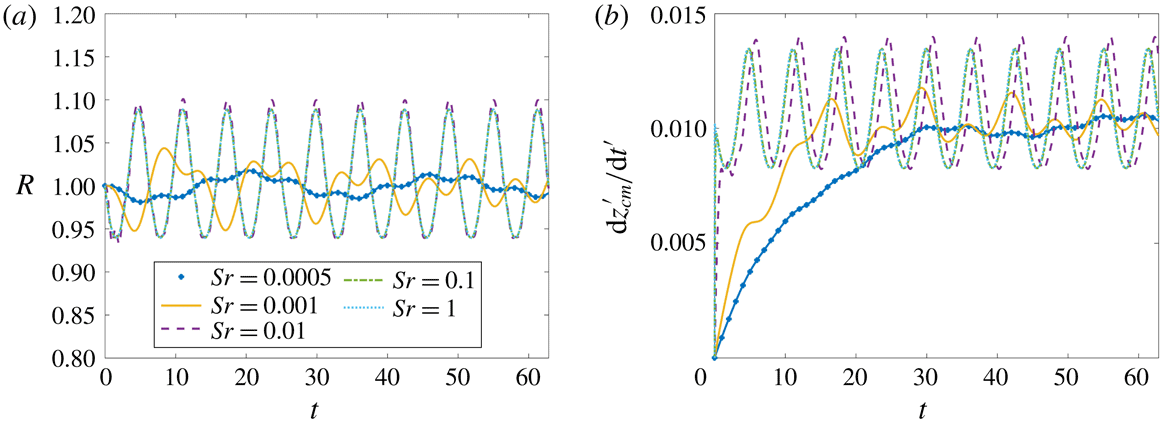
As will be shown below, the mobilization of the bubble becomes maximized when the imposed frequency of the acoustic field, or Sr in dimensionless terms, is close to the natural frequency that is calculated by (3.29) or its equivalent (3.30).
When it comes to the flow of a viscoplastic material, it is always important to investigate the existence of an unyielded region and the position/shape of the possible yield surface. This limiting case can be used to draw some interesting conclusions regarding the flow of the viscoplastic material that surrounds the bubble. In the absence of any translation, the velocity potential is simply given by
 $\unicode[STIX]{x1D711}={\dot{R}}R^{2}/r$
, which can be introduced into (3.3) to evaluate the stress tensor, and subsequently its dimensional second invariant is given by
$\unicode[STIX]{x1D711}={\dot{R}}R^{2}/r$
, which can be introduced into (3.3) to evaluate the stress tensor, and subsequently its dimensional second invariant is given by
 $$\begin{eqnarray}\displaystyle \Vert \unicode[STIX]{x1D64F}\Vert =2\sqrt{3}\unicode[STIX]{x1D707}\left|\frac{R^{2}{\dot{R}}}{r^{3}}\right|+\unicode[STIX]{x1D70F}_{y}. & & \displaystyle\end{eqnarray}$$
According to the Von Mises criterion, an unyielded region exists in areas where the following inequality is satisfied:
 $\Vert \unicode[STIX]{x1D64F}\Vert \leqslant \unicode[STIX]{x1D70F}_{y}$
. When the bubble expands or contracts, i.e.
$\Vert \unicode[STIX]{x1D64F}\Vert \leqslant \unicode[STIX]{x1D70F}_{y}$
. When the bubble expands or contracts, i.e.
 ${\dot{R}}\neq 0$
,
${\dot{R}}\neq 0$
,
 $\Vert \unicode[STIX]{x1D64F}\Vert >\unicode[STIX]{x1D70F}_{y}$
, and therefore it becomes evident that in the case of sphero-symmetric bubble oscillation a true unyielded region cannot exist except for the time instants that
$\Vert \unicode[STIX]{x1D64F}\Vert >\unicode[STIX]{x1D70F}_{y}$
, and therefore it becomes evident that in the case of sphero-symmetric bubble oscillation a true unyielded region cannot exist except for the time instants that
 ${\dot{R}}$
is equal to zero, i.e. the time of maximum expansion or contraction of the bubble. However, since the yielding of the material is typically related to the buildup or breakdown of a specific structure which requires a finite amount of time, we conclude that practically unyielded regions do not exist in the case of a sphero-symmetric bubble oscillation. The non-existence of an unyielded region in this type of flow can be attributed to the incompressibility of the material. As the bubble expands sphero-symmetrically, there will always be flow in the radial direction as the bubble displaces the material while it expands or due to the fact that the liquid follows the contraction of the bubble to occupy the empty space.
${\dot{R}}$
is equal to zero, i.e. the time of maximum expansion or contraction of the bubble. However, since the yielding of the material is typically related to the buildup or breakdown of a specific structure which requires a finite amount of time, we conclude that practically unyielded regions do not exist in the case of a sphero-symmetric bubble oscillation. The non-existence of an unyielded region in this type of flow can be attributed to the incompressibility of the material. As the bubble expands sphero-symmetrically, there will always be flow in the radial direction as the bubble displaces the material while it expands or due to the fact that the liquid follows the contraction of the bubble to occupy the empty space.
4 Two-dimensional axisymmetric finite element model
In this part of our work, we will develop a more rigorous model assuming axial symmetry and fully taking into account the deformability of the bubble. Since the dynamics as well as the motion of the bubble in the viscoplastic medium will be driven by the combined effect of buoyancy and the externally imposed acoustic pressure field, the time-dependent velocity of the bubble centre of mass,
 $U_{b}(t)$
, its position and shape will have to be evaluated through transient simulations. A boundary-fitted finite element model is developed for that purpose.
$U_{b}(t)$
, its position and shape will have to be evaluated through transient simulations. A boundary-fitted finite element model is developed for that purpose.
Considering the case of an axisymmetric bubble, we assume that the bubble motion is aligned with the
 $z$
-axis of our coordinate system (see figure 1
b). Moreover, the origin of the cylindrical coordinate system is set at the initial position of the centre of mass of the bubble, i.e.
$z$
-axis of our coordinate system (see figure 1
b). Moreover, the origin of the cylindrical coordinate system is set at the initial position of the centre of mass of the bubble, i.e.
 $z_{cm}(t=0)=0$
.
$z_{cm}(t=0)=0$
.
The flow in the viscoplastic material is governed by the momentum and mass conservation equations, which in dimensionless form and under the arbitrary Lagrangian–Eulerian description become
 $$\begin{eqnarray}\displaystyle & \displaystyle Ar\left[Sr^{-1}\frac{\unicode[STIX]{x2202}\boldsymbol{u}}{\unicode[STIX]{x2202}t}+(\boldsymbol{u}-\boldsymbol{u}_{g})\boldsymbol{\cdot }\unicode[STIX]{x1D735}\boldsymbol{u}\right]-\unicode[STIX]{x1D735}\boldsymbol{\cdot }(-p\unicode[STIX]{x1D644}+\unicode[STIX]{x1D64F})+\boldsymbol{e}_{z}=0, & \displaystyle\end{eqnarray}$$
 $$\begin{eqnarray}\displaystyle & \displaystyle \unicode[STIX]{x1D735}\boldsymbol{\cdot }\boldsymbol{u}=0, & \displaystyle\end{eqnarray}$$
where
 $\boldsymbol{u}=(u_{r},u_{z})$
and
$\boldsymbol{u}=(u_{r},u_{z})$
and
 $p$
denote the dimensionless velocity field and pressure, respectively,
$p$
denote the dimensionless velocity field and pressure, respectively,
 $\unicode[STIX]{x1D64F}$
is the dimensionless stress tensor and
$\unicode[STIX]{x1D64F}$
is the dimensionless stress tensor and
 $\unicode[STIX]{x1D735}$
is the gradient operator. Parameter
$\unicode[STIX]{x1D735}$
is the gradient operator. Parameter
 $\boldsymbol{u}_{g}=Sr^{-1}\unicode[STIX]{x2202}\boldsymbol{r}_{g}/\unicode[STIX]{x2202}t$
is the velocity of the mesh nodes on the flow domain, where
$\boldsymbol{u}_{g}=Sr^{-1}\unicode[STIX]{x2202}\boldsymbol{r}_{g}/\unicode[STIX]{x2202}t$
is the velocity of the mesh nodes on the flow domain, where
 $\boldsymbol{r}_{g}$
denotes the position vector of the mesh nodes. We use the same scaling as that described in the previous section.
$\boldsymbol{r}_{g}$
denotes the position vector of the mesh nodes. We use the same scaling as that described in the previous section.
To complete the description, a constitutive equation that describes the rheology of the fluid is required, and as such we will employ the continuous constitutive equation proposed by Papanastasiou (Reference Papanastasiou1987):
 $$\begin{eqnarray}\displaystyle \unicode[STIX]{x1D64F}=\left(1+Bn\frac{1-\text{e}^{-N\Vert \unicode[STIX]{x1D71E}\Vert }}{\Vert \unicode[STIX]{x1D71E}\Vert }\right)\unicode[STIX]{x1D71E}, & & \displaystyle\end{eqnarray}$$
where
 $N$
is the dimensionless stress growth exponent. In the simulations to be presented in this paper and after careful evaluation, we have chosen the value of
$N$
is the dimensionless stress growth exponent. In the simulations to be presented in this paper and after careful evaluation, we have chosen the value of
 $N$
to be in the range
$N$
to be in the range
 $10^{4}{-}10^{6}$
in order to neither affect the yield surface by overly decreasing
$10^{4}{-}10^{6}$
in order to neither affect the yield surface by overly decreasing
 $N$
nor produce numerical instabilities or stiff equations by increasing it. As shown in Dimakopoulos et al. (Reference Dimakopoulos, Pavlidis and Tsamopoulos2013) such values of
$N$
nor produce numerical instabilities or stiff equations by increasing it. As shown in Dimakopoulos et al. (Reference Dimakopoulos, Pavlidis and Tsamopoulos2013) such values of
 $N$
provide results with reasonable agreement with the augmented Lagrangian method.
$N$
provide results with reasonable agreement with the augmented Lagrangian method.
Along the free surface of the bubble, the velocity field should satisfy a local force balance between capillary forces and viscous stresses in the liquid and pressure inside the bubble:
 $$\begin{eqnarray}\displaystyle \boldsymbol{n}\boldsymbol{\cdot }(-p\unicode[STIX]{x1D644}+\unicode[STIX]{x1D64F})=-p_{g}(t)\boldsymbol{n}+Bo^{-1}\unicode[STIX]{x1D705}\boldsymbol{n}, & & \displaystyle\end{eqnarray}$$
where
 $\boldsymbol{n}$
denotes the outward unit normal to the free surface and
$\boldsymbol{n}$
denotes the outward unit normal to the free surface and
 $\unicode[STIX]{x1D705}$
is its mean curvature which is defined as
$\unicode[STIX]{x1D705}$
is its mean curvature which is defined as
 $$\begin{eqnarray}\displaystyle \unicode[STIX]{x1D705}=-\unicode[STIX]{x1D735}_{s}\boldsymbol{\cdot }\boldsymbol{n},\quad \unicode[STIX]{x1D735}_{s}=(\unicode[STIX]{x1D644}-A\boldsymbol{A})\boldsymbol{\cdot }\unicode[STIX]{x1D735}. & & \displaystyle\end{eqnarray}$$
Here
 $p_{g}(t)$
denotes the dimensionless gas pressure in the bubble given by
$p_{g}(t)$
denotes the dimensionless gas pressure in the bubble given by
 $$\begin{eqnarray}\displaystyle p_{g}(t)=c_{o}v(t)^{-k}. & & \displaystyle\end{eqnarray}$$
Here
 $c_{o}=p_{go}v_{o}^{k}$
, where
$c_{o}=p_{go}v_{o}^{k}$
, where
 $p_{go}=p_{r}+2Bo^{-1}$
is the dimensionless gas pressure in the bubble at equilibrium and
$p_{go}=p_{r}+2Bo^{-1}$
is the dimensionless gas pressure in the bubble at equilibrium and
 $v_{o}=4\unicode[STIX]{x03C0}/3$
its corresponding dimensionless volume. Volume
$v_{o}=4\unicode[STIX]{x03C0}/3$
its corresponding dimensionless volume. Volume
 $v(t)$
is the dimensionless bubble volume at any time instant. The bubble volume can be evaluated efficiently using the following expression:
$v(t)$
is the dimensionless bubble volume at any time instant. The bubble volume can be evaluated efficiently using the following expression:
 $$\begin{eqnarray}\displaystyle v(t)=-\frac{1}{3}\int \boldsymbol{r}\boldsymbol{\cdot }\boldsymbol{n}\,\text{d}S_{1}, & & \displaystyle\end{eqnarray}$$
where
 $\boldsymbol{r}$
denotes the position vector along the liquid–gas interface in the cylindrical coordinate system. Here, we have used the divergence theorem to turn the volume integral into a surface integral that can be evaluated along the liquid–gas interface.
$\boldsymbol{r}$
denotes the position vector along the liquid–gas interface in the cylindrical coordinate system. Here, we have used the divergence theorem to turn the volume integral into a surface integral that can be evaluated along the liquid–gas interface.
On the axis of symmetry (
 $r=0$
) we apply the usual symmetry conditions, i.e.
$r=0$
) we apply the usual symmetry conditions, i.e.
 $u_{r}=0$
and
$u_{r}=0$
and
 $\unicode[STIX]{x2202}u_{r}/\unicode[STIX]{x2202}r=0$
. Far from the bubble, we employ the open boundary condition introduced by Papanastasiou, Malamataris & Ellwood (Reference Papanastasiou, Malamataris and Ellwood1992). According to this scheme, sufficiently far from the bubble, at distance
$\unicode[STIX]{x2202}u_{r}/\unicode[STIX]{x2202}r=0$
. Far from the bubble, we employ the open boundary condition introduced by Papanastasiou, Malamataris & Ellwood (Reference Papanastasiou, Malamataris and Ellwood1992). According to this scheme, sufficiently far from the bubble, at distance
 $R_{\infty }$
from the bubble centre of mass, the axial component of the fluid velocity is imposed at one node of the outer boundary, i.e. by imposing
$R_{\infty }$
from the bubble centre of mass, the axial component of the fluid velocity is imposed at one node of the outer boundary, i.e. by imposing
 $u_{z}=0$
at
$u_{z}=0$
at
 $(r,z)=(0,R_{\infty }+z_{cm})$
, while the rest are simply calculated from the weak form of the equations (e.g. see Dimakopoulos et al.
Reference Dimakopoulos, Karapetsas, Malamataris and Mitsoulis2012; Fraggedakis, Dimakopoulos & Tsamopoulos Reference Fraggedakis, Dimakopoulos and Tsamopoulos2016c
); a rigorous explanation as to why this treatment of the boundary conditions works is given by Renardy (Reference Renardy1997). In all cases to be presented below, the value of
$(r,z)=(0,R_{\infty }+z_{cm})$
, while the rest are simply calculated from the weak form of the equations (e.g. see Dimakopoulos et al.
Reference Dimakopoulos, Karapetsas, Malamataris and Mitsoulis2012; Fraggedakis, Dimakopoulos & Tsamopoulos Reference Fraggedakis, Dimakopoulos and Tsamopoulos2016c
); a rigorous explanation as to why this treatment of the boundary conditions works is given by Renardy (Reference Renardy1997). In all cases to be presented below, the value of
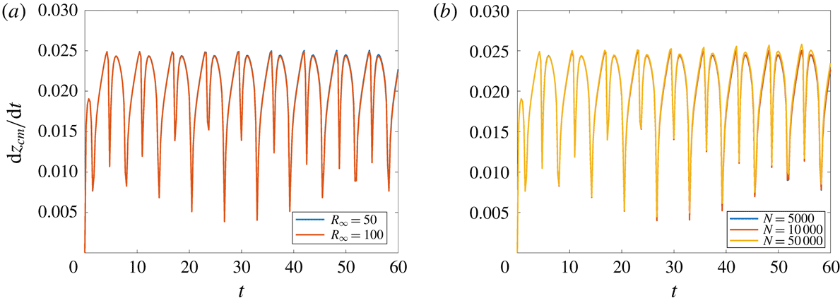
 $R_{\infty }$
has been chosen so that it does not affect the solution. Far from the bubble at the equatorial plane (
$R_{\infty }$
has been chosen so that it does not affect the solution. Far from the bubble at the equatorial plane (
 $r=R_{\infty },z=z_{cm}$
) the imposed pressure is given by
$r=R_{\infty },z=z_{cm}$
) the imposed pressure is given by
 $$\begin{eqnarray}\displaystyle p_{\infty }(z,t)=p_{r}(1+a\sin (t))-z, & & \displaystyle\end{eqnarray}$$
where
 $a$
is the dimensionless pressure amplitude. Finally, the position of the bubble centre at every time instant is evaluated using the following expression:
$a$
is the dimensionless pressure amplitude. Finally, the position of the bubble centre at every time instant is evaluated using the following expression:
 $$\begin{eqnarray}\displaystyle z_{cm}(t)=\int z\,\text{d}V\left/\int \,\text{d}V\right.=\frac{3}{4}\int z\boldsymbol{r}\boldsymbol{\cdot }\boldsymbol{n}\,\text{d}S_{1}\left/\int \boldsymbol{r}\boldsymbol{\cdot }\boldsymbol{n}\,\text{d}S_{1}\right.. & & \displaystyle\end{eqnarray}$$
Here, we have also used the divergence theorem to turn the volume integrals into surface integrals that can be evaluated along the liquid–gas interface.
As in our previous work, the above set of equations is combined with an elliptic grid generation scheme (see Dimakopoulos & Tsamopoulos Reference Dimakopoulos and Tsamopoulos2003) which consists of a system of quasi-elliptic partial differential equations, capable of generating a boundary-fitted discretization of the deforming domain occupied by the liquid (see Tsamopoulos et al. (Reference Tsamopoulos, Dimakopoulos, Chatzidai, Karapetsas and Pavlidis2008) for details). This is achieved by imposing as boundary condition the kinematic equation along the moving liquid–gas interface:
 $$\begin{eqnarray}\displaystyle (\boldsymbol{u}-\boldsymbol{u}_{g})\boldsymbol{\cdot }\boldsymbol{n}=0. & & \displaystyle\end{eqnarray}$$
Moreover, we apply the following boundary conditions along the outer boundary so that our physical domain is able to follow the rising motion of the bubble:
 $$\begin{eqnarray}\displaystyle & \displaystyle z(t)=z_{o}+z_{cm}(t), & \displaystyle\end{eqnarray}$$
 $$\begin{eqnarray}\displaystyle & \displaystyle r(t)=\sqrt{R_{\infty }^{2}-z(t)^{2}}, & \displaystyle\end{eqnarray}$$
where
 $z_{o}$
denotes the axial position of the nodes at
$z_{o}$
denotes the axial position of the nodes at
 $t=0$
. In order to solve numerically the governing equations along with the elliptic grid equations, we used the mixed finite element method. The set of discretized differential equations is integrated in time with the implicit Euler method while the initial time step was set to
$t=0$
. In order to solve numerically the governing equations along with the elliptic grid equations, we used the mixed finite element method. The set of discretized differential equations is integrated in time with the implicit Euler method while the initial time step was set to
 $10^{-4}$
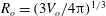
. In order to resolve adequately the flow, the mesh is refined around the liquid–gas interface (Chatzidai et al.
Reference Chatzidai, Giannousakis, Dimakopoulos and Tsamopoulos2009); our typical mesh consists of 20 000 triangular elements and numerical checks showed that increasing the number of elements further led to negligible changes. The code has been thoroughly validated against our previous work (Tsamopoulos et al.
Reference Tsamopoulos, Dimakopoulos, Chatzidai, Karapetsas and Pavlidis2008).
$10^{-4}$
. In order to resolve adequately the flow, the mesh is refined around the liquid–gas interface (Chatzidai et al.
Reference Chatzidai, Giannousakis, Dimakopoulos and Tsamopoulos2009); our typical mesh consists of 20 000 triangular elements and numerical checks showed that increasing the number of elements further led to negligible changes. The code has been thoroughly validated against our previous work (Tsamopoulos et al.
Reference Tsamopoulos, Dimakopoulos, Chatzidai, Karapetsas and Pavlidis2008).
5 Results and discussion
For the purpose of the present study, we place our focus on the parameter range which is most relevant to an important engineering application, i.e. the process of de-aeration and consolidation of concrete, since it is encountered in everyday life. Nevertheless, it is important to note that the results of the present analysis will have a much more general applicability than this specific application. For this purpose, we have obtained numerical solutions over a wide range of parameter values, while the ‘base’ case has broadly the typical values shown in table 1.
Table 1. Parameter values which correspond to the ‘base’ case considered in this study.
These values correspond to a bubble of millimetric size entrained in a dense liquid such as fresh concrete at a depth of 1 m and an imposed frequency of 200 Hz; more details of the corresponding physical constants can be found in appendix A. The simulations for all cases presented below were performed until several periods of the bubble oscillations were completed, to ensure that the oscillations have reached a steady state.
5.1 Sphero-symmetric bubble oscillations: one-dimensional reduced-order model
We begin our study with a discussion about the predictions of the sphero-symmetric model that we developed in § 3. Note that for all simulations presented below, we have considered
 $R_{\infty }=10^{4}$
; considering values one order of magnitude lower or higher than this value led to negligible differences. First, we examine in figure 2 the effect of the yield stress by varying the value of Bn. In this figure we plot the evolution of the dimensionless velocity of the bubble,
$R_{\infty }=10^{4}$
; considering values one order of magnitude lower or higher than this value led to negligible differences. First, we examine in figure 2 the effect of the yield stress by varying the value of Bn. In this figure we plot the evolution of the dimensionless velocity of the bubble,
 $\text{d}z_{cm}/\text{d}t$
(see figure 2
a), along with the position of its centre of mass,
$\text{d}z_{cm}/\text{d}t$
(see figure 2
a), along with the position of its centre of mass,
 $z_{cm}$
(see figure 2
b). It is already known for the case of steady bubble rise under a static pressure field that motion takes place below a critical value of Bn and the bubble rise velocity decreases with increasing viscoplasticity of the material because of the increasing effective viscosity. As shown in figure 2, a similar behaviour is encountered when the bubble is subjected to an acoustic field resulting in deceleration of the bubble with increasing yield stress. For
$z_{cm}$
(see figure 2
b). It is already known for the case of steady bubble rise under a static pressure field that motion takes place below a critical value of Bn and the bubble rise velocity decreases with increasing viscoplasticity of the material because of the increasing effective viscosity. As shown in figure 2, a similar behaviour is encountered when the bubble is subjected to an acoustic field resulting in deceleration of the bubble with increasing yield stress. For
 $Bn=0.1$
, the bubble covers a distance equal to 0.3 times the bubble radius after approximately 10 cycles of pressure oscillation (at
$Bn=0.1$
, the bubble covers a distance equal to 0.3 times the bubble radius after approximately 10 cycles of pressure oscillation (at
 $t=61.53$
), whereas in the case of a Newtonian liquid the same distance is covered at
$t=61.53$
), whereas in the case of a Newtonian liquid the same distance is covered at
 $t=26.75$
; assuming that the imposed frequency is 200 Hz the corresponding time in dimensional terms would be 0.308 and 0.134 s, respectively.
$t=26.75$
; assuming that the imposed frequency is 200 Hz the corresponding time in dimensional terms would be 0.308 and 0.134 s, respectively.

Figure 2. Evolution of (a) bubble rise velocity and (b) position of bubble centre of mass for different values of Bn. The other parameter values are given in table 1.
The presence of the acoustic field, though, causes volume oscillations of the bubble (see figure 3
a for the evolution of the bubble radius), due to its compressibility. The volume oscillation modifies the stress in the liquid surrounding the bubble and thus allows overcoming the yield stress of the material. Therefore, even though the present simplified model predicts that in the presence of a static pressure field the bubble will become entrapped for
 $Bn=0.175$
(see (3.26)), we find that in the presence of an acoustic field bubble motion is still possible beyond this critical value, i.e. for
$Bn=0.175$
(see (3.26)), we find that in the presence of an acoustic field bubble motion is still possible beyond this critical value, i.e. for
 $Bn=0.18$
. For this value of Bn, the bubble rises during the expanding phase of the bubble whereas remains stagnant when the bubble contracts. Eventually, for even higher values of Bn, e.g. for
$Bn=0.18$
. For this value of Bn, the bubble rises during the expanding phase of the bubble whereas remains stagnant when the bubble contracts. Eventually, for even higher values of Bn, e.g. for
 $Bn=0.2$
, the model predicts that the rise velocity becomes equal to zero and thus the bubble is entrapped.
$Bn=0.2$
, the model predicts that the rise velocity becomes equal to zero and thus the bubble is entrapped.

Figure 3. Evolution of (a) bubble radius and (b) position of bubble centre of mass for different values of Bo. The other parameter values are given in table 1.
It is noteworthy that the effect of Bn on the amplitude of volume oscillations is negligible (not shown here for conciseness). However, as shown in figure 3(a), the amplitude of radial oscillations depends strongly on the surface tension of the liquid–air interface, and thus on the value of the Bond number, which acts as a restoring force to maintain the bubble shape. Higher values of Bo result in bubbles which are susceptible to larger volume oscillations leading to a slight increase of their mobility; the latter is not significant for the specific parameter values that we have considered (see figure 3 b).
The amplitude of volume oscillations also depends significantly on the amplitude of the imposed pressure oscillations,
 $a$
, far from the bubble (see figure 4
a). For small values of
$a$
, far from the bubble (see figure 4
a). For small values of
 $a$
, the difference in the bubble volume is not significant between the two phases of the flow, i.e. contraction and expansion. On increasing the amplitude,
$a$
, the difference in the bubble volume is not significant between the two phases of the flow, i.e. contraction and expansion. On increasing the amplitude,
 $a$
, this symmetry breaks and the bubble undergoes substantial growth which is followed by limited contraction. For amplitude
$a$
, this symmetry breaks and the bubble undergoes substantial growth which is followed by limited contraction. For amplitude
 $a=0.7$
, i.e. 70 % of the reference pressure, during expansion the bubble radius increases by approximately 33 % which corresponds to an increase in bubble volume of
$a=0.7$
, i.e. 70 % of the reference pressure, during expansion the bubble radius increases by approximately 33 % which corresponds to an increase in bubble volume of
 ${\sim}235\,\%$
. On the other hand, during contraction the minimum bubble radius reaches
${\sim}235\,\%$
. On the other hand, during contraction the minimum bubble radius reaches
 ${\sim}88\,\%$
of its initial value, i.e. the volume decreases at most by
${\sim}88\,\%$
of its initial value, i.e. the volume decreases at most by
 ${\sim}32\%$
. As expected, increasing the amplitude of bubble oscillations leads to an increase of the mobility of the bubble (see figure 4
b).
${\sim}32\%$
. As expected, increasing the amplitude of bubble oscillations leads to an increase of the mobility of the bubble (see figure 4
b).

Figure 4. Evolution of (a) bubble radius and (b) position of bubble centre of mass for different amplitudes of pressure oscillation. The other parameter values are given in table 1.
In figure 5 we examine the effect of Ar, which is a measure of the importance of inertia in our system, on the bubble rise velocity. At this point, it is important to mention that the particular selection of our scaling poses an inherent difficulty in the interpretation of our results when varying Ar while keeping fixed the value of Sr. These two numbers are related to each other according to the following expression:
 $Ar=Sr^{2}f^{2}R_{o}/g$
. Therefore, assuming that the characteristic time is fixed, i.e. a constant imposed frequency, would imply that bubbles of different radii are examined with fixed Sr and increasing values of Ar. Since lengths are scaled with
$Ar=Sr^{2}f^{2}R_{o}/g$
. Therefore, assuming that the characteristic time is fixed, i.e. a constant imposed frequency, would imply that bubbles of different radii are examined with fixed Sr and increasing values of Ar. Since lengths are scaled with
 $R_{o}$
it would be difficult to evaluate the dependence of the actual bubble rise velocity on Ar. To overcome this problem, we introduce an alternative scaling for the length, using the viscous length scale
$R_{o}$
it would be difficult to evaluate the dependence of the actual bubble rise velocity on Ar. To overcome this problem, we introduce an alternative scaling for the length, using the viscous length scale
 $l_{v}=(\unicode[STIX]{x1D707}^{2}/\unicode[STIX]{x1D70C}^{2}g)^{1/3}$
, and for time, using the viscous time scale
$l_{v}=(\unicode[STIX]{x1D707}^{2}/\unicode[STIX]{x1D70C}^{2}g)^{1/3}$
, and for time, using the viscous time scale
 $t_{v}=(\unicode[STIX]{x1D707}/\unicode[STIX]{x1D70C}g^{2})^{1/3}$
, which are solely based on liquid properties. Assuming a liquid with density
$t_{v}=(\unicode[STIX]{x1D707}/\unicode[STIX]{x1D70C}g^{2})^{1/3}$
, which are solely based on liquid properties. Assuming a liquid with density
 $2400~\text{kg}~\text{m}^{-3}$
and viscosity 1 Pa s, we get that
$2400~\text{kg}~\text{m}^{-3}$
and viscosity 1 Pa s, we get that
 $t_{v}=0.0163~\text{s}$
,
$t_{v}=0.0163~\text{s}$
,
 $l_{v}=2.605~\text{mm}$
and
$l_{v}=2.605~\text{mm}$
and
 $l_{v}/t_{v}=0.16~\text{m}~\text{s}^{-1}$
. We denote the new dimensionless position of the centre of mass and dimensionless time as
$l_{v}/t_{v}=0.16~\text{m}~\text{s}^{-1}$
. We denote the new dimensionless position of the centre of mass and dimensionless time as
 $z_{cm}^{\prime }$
and
$z_{cm}^{\prime }$
and
 $t^{\prime }$
, respectively; accordingly, the bubble rise velocity,
$t^{\prime }$
, respectively; accordingly, the bubble rise velocity,
 $\text{d}z_{cm}^{\prime }/\text{d}t^{\prime }$
, has been scaled with
$\text{d}z_{cm}^{\prime }/\text{d}t^{\prime }$
, has been scaled with
 $l_{v}/t_{v}=(\unicode[STIX]{x1D707}g/\unicode[STIX]{x1D70C})^{1/3}$
. The new scaling allows a direct comparison of the bubble rise velocity for different values of Ar. As depicted in figure 5, increasing the value of Ar results in a considerable speeding up of the bubble rising motion due to the increased effect of buoyancy. Note that in figure 5(a)
$l_{v}/t_{v}=(\unicode[STIX]{x1D707}g/\unicode[STIX]{x1D70C})^{1/3}$
. The new scaling allows a direct comparison of the bubble rise velocity for different values of Ar. As depicted in figure 5, increasing the value of Ar results in a considerable speeding up of the bubble rising motion due to the increased effect of buoyancy. Note that in figure 5(a)
 $\text{d}z_{cm}^{\prime }/\text{d}t^{\prime }$
is plotted against
$\text{d}z_{cm}^{\prime }/\text{d}t^{\prime }$
is plotted against
 $t$
to clearly depict the dependence of the rise velocity for all values of Ar for the same number of pressure cycles, whereas in figure 5(b) we prefer to plot
$t$
to clearly depict the dependence of the rise velocity for all values of Ar for the same number of pressure cycles, whereas in figure 5(b) we prefer to plot
 $z_{cm}^{\prime }$
versus
$z_{cm}^{\prime }$
versus
 $t^{\prime }$
since from the slope of these curves it is possible to infer the rise velocity of the bubble,
$t^{\prime }$
since from the slope of these curves it is possible to infer the rise velocity of the bubble,
 $\text{d}z_{cm}^{\prime }/\text{d}t^{\prime }$
. Moreover, as shown in figure 5(a), nonlinear effects become prominent for the highest value of Ar that we have considered, i.e. for
$\text{d}z_{cm}^{\prime }/\text{d}t^{\prime }$
. Moreover, as shown in figure 5(a), nonlinear effects become prominent for the highest value of Ar that we have considered, i.e. for
 $Ar=10$
.
$Ar=10$
.

Figure 5. Evolution of (a) bubble rise velocity and (b) position of bubble centre of mass for different values of Ar;
 $t$
and
$t$
and
 $t^{\prime }$
denote the time scaled with
$t^{\prime }$
denote the time scaled with
 $f^{-1}$
and
$f^{-1}$
and
 $t_{v}$
, respectively. The other parameter values are given in table 1.
$t_{v}$
, respectively. The other parameter values are given in table 1.
The effect of Sr, over a wide range of values, is examined in figure 6. For very small values of Sr, i.e.
 $Sr=0.0005$
, which correspond to high-frequency pressure oscillations, the bubble does not have enough time to adjust to the changing pressure field and therefore the amplitude of volume oscillations is reduced (see figure 6
a) while the rise velocity (see figure 6
b) soon approaches the steady rise velocity for a static pressure field
$Sr=0.0005$
, which correspond to high-frequency pressure oscillations, the bubble does not have enough time to adjust to the changing pressure field and therefore the amplitude of volume oscillations is reduced (see figure 6
a) while the rise velocity (see figure 6
b) soon approaches the steady rise velocity for a static pressure field
 $\text{d}z_{cm}^{\prime }/\text{d}t^{\prime }=(1/9)(1-(3/4)\unicode[STIX]{x1D712}Bn)Ar^{2/3}\approx 0.0102$
; the latter expression has been derived using (3.24) assuming
$\text{d}z_{cm}^{\prime }/\text{d}t^{\prime }=(1/9)(1-(3/4)\unicode[STIX]{x1D712}Bn)Ar^{2/3}\approx 0.0102$
; the latter expression has been derived using (3.24) assuming
 ${\dot{R}}=0$
,
${\dot{R}}=0$
,
 $\ddot{z}=0$
and
$\ddot{z}=0$
and
 ${\dot{z}}>0$
. The amplitude of radial oscillations increases with increasing Sr indicating that the resonance frequency of the system should be in the regime
${\dot{z}}>0$
. The amplitude of radial oscillations increases with increasing Sr indicating that the resonance frequency of the system should be in the regime
 $0.001<Sr<0.01$
. For even higher values of Sr, i.e.
$0.001<Sr<0.01$
. For even higher values of Sr, i.e.
 $Sr\geqslant 0.1$
, an asymptotic regime is reached where the behaviour of the system is determined only by the amplitude of the imposed pressure oscillations.
$Sr\geqslant 0.1$
, an asymptotic regime is reached where the behaviour of the system is determined only by the amplitude of the imposed pressure oscillations.

Figure 6. Evolution of (a) bubble radius and (b) bubble rise velocity for different values of Sr. The other parameter values are given in table 1.

Figure 7. Evolution of (a) bubble rise velocity and (b) bubble radius for values of Sr which correspond to frequencies in the region of the resonance frequency. The other parameter values are given in table 1.
As discussed in § 3.1.2, Sr which corresponds to the natural frequency of a pulsating bubble in the absence of buoyancy effects is given by (3.30). For the parameter values that we consider as our base case, this equation predicts that resonance should take place for
 $Sr\approx 0.002185$
. Our numerical simulations indicate that this is a good approximation of the natural frequency even in our case where buoyancy is important. This is clearly demonstrated in figure 7 where we plot the evolution of the rise velocity,
$Sr\approx 0.002185$
. Our numerical simulations indicate that this is a good approximation of the natural frequency even in our case where buoyancy is important. This is clearly demonstrated in figure 7 where we plot the evolution of the rise velocity,
 $\text{d}z_{cm}^{\prime }/\text{d}t^{\prime }$
, and bubble radius,
$\text{d}z_{cm}^{\prime }/\text{d}t^{\prime }$
, and bubble radius,
 $R$
, with time for three different values of Sr. Near resonance the volume oscillations become maximized affecting the mobility of the bubble in the viscoplastic material through two different mechanisms. The first mechanism is related to the increased effect of buoyancy due to the maximized bubble volume during the expansion phase that can be attained near resonance. The second mechanism is related to the rapid growth of the bubble size inducing high shear rates in the liquid surrounding the bubble which results in decreased effective viscosity of the material.
$R$
, with time for three different values of Sr. Near resonance the volume oscillations become maximized affecting the mobility of the bubble in the viscoplastic material through two different mechanisms. The first mechanism is related to the increased effect of buoyancy due to the maximized bubble volume during the expansion phase that can be attained near resonance. The second mechanism is related to the rapid growth of the bubble size inducing high shear rates in the liquid surrounding the bubble which results in decreased effective viscosity of the material.
These two mechanisms are always present when a bubble is subjected to an acoustic field. We have already seen in figure 2 that even for conditions far from resonance the bubble is able to rise for values of Bn slightly higher than the critical value. However, the effect of these mechanisms on the stress field is significantly more near resonance, and, as shown in figure 8, our simplified model predicts that for
 $Sr=0.002185$
the range of Bn for which bubble motion is possible widens considerably, i.e. even for
$Sr=0.002185$
the range of Bn for which bubble motion is possible widens considerably, i.e. even for
 $Bn=0.25$
the bubble rises slowly whereas bubble entrapment is predicted for
$Bn=0.25$
the bubble rises slowly whereas bubble entrapment is predicted for
 $Bn=0.175$
in the case of static pressure field.
$Bn=0.175$
in the case of static pressure field.

Figure 8. Evolution of the position of bubble centre of mass,
 $z_{cm}$
, for different values of Bn. The value of
$z_{cm}$
, for different values of Bn. The value of
 $Sr=0.002185$
corresponds to an imposed frequency close to the natural frequency of the system. The other parameter values are given in table 1.
$Sr=0.002185$
corresponds to an imposed frequency close to the natural frequency of the system. The other parameter values are given in table 1.
5.2 Axisymmetric deformable bubble: two-dimensional model
So far, we have examined in detail the predictions of a simplified sphero-symmetric model. In this part of our work, we perform simulations using a more rigorous model that fully takes into account bubble deformability and the flow field surrounding the bubble, assuming axial symmetry only. The details of the model are presented in § 4. Note that for all the simulations that will be presented below, we have considered
 $R_{\infty }=50$
; considering values higher than this value (e.g.
$R_{\infty }=50$
; considering values higher than this value (e.g.
 $R_{\infty }=100$
) led to negligible differences (see appendix B). Moreover, the exponential factor,
$R_{\infty }=100$
) led to negligible differences (see appendix B). Moreover, the exponential factor,
 $N$
, which arises in (4.3) was considered to be equal to
$N$
, which arises in (4.3) was considered to be equal to
 $10^{4}$
for all the simulations that will be presented below, in line with our previous work (Tsamopoulos et al.
Reference Tsamopoulos, Dimakopoulos, Chatzidai, Karapetsas and Pavlidis2008); considering values higher than this value (e.g.
$10^{4}$
for all the simulations that will be presented below, in line with our previous work (Tsamopoulos et al.
Reference Tsamopoulos, Dimakopoulos, Chatzidai, Karapetsas and Pavlidis2008); considering values higher than this value (e.g.
 $N=5\times 10^{4}$
) led to negligible differences in the dynamics of bubble motion (see appendix B).
$N=5\times 10^{4}$
) led to negligible differences in the dynamics of bubble motion (see appendix B).
Below, we determine the yield surface as the location where
 $\Vert \unicode[STIX]{x1D64F}\Vert =Bn=0.1$
, employing the Von Mises criterion. It is important to keep in mind, though, that according to the Papanastasiou model, even for
$\Vert \unicode[STIX]{x1D64F}\Vert =Bn=0.1$
, employing the Von Mises criterion. It is important to keep in mind, though, that according to the Papanastasiou model, even for
 $\Vert \unicode[STIX]{x1D64F}\Vert <Bn$
, finite motion of the material is allowed, albeit with very large viscosity, and therefore using this model it is not possible to predict a true zone of unyielded material. In fact, in our case, given the radial character of the flow and the fact that the liquid is considered to be incompressible, we expect that the radial velocity will acquire small but finite values even very far from the bubble and therefore we expect a material following the Papanastasiou model, and thus exhibiting no elasticity, should actually yield. On the other hand, in the case of elastoviscoplastic materials, the material could exhibit true unyielded zones, since in this case the material could also experience an elastic solid deformation. Therefore, in the discussion that follows, we will still refer to a yield surface but with the understanding that this does not correspond to a true boundary between truly yielded and unyielded domains. It will rather be used as a convenient way to study the evolution and visualize regions with relatively low viscosity (which hereafter we will refer to as yielded regions) and regions with much higher viscosity (which hereafter we will refer to as unyielded regions). It should also be noted that the position of this pseudo-yield surface is quite sensitive to the value of
$\Vert \unicode[STIX]{x1D64F}\Vert <Bn$
, finite motion of the material is allowed, albeit with very large viscosity, and therefore using this model it is not possible to predict a true zone of unyielded material. In fact, in our case, given the radial character of the flow and the fact that the liquid is considered to be incompressible, we expect that the radial velocity will acquire small but finite values even very far from the bubble and therefore we expect a material following the Papanastasiou model, and thus exhibiting no elasticity, should actually yield. On the other hand, in the case of elastoviscoplastic materials, the material could exhibit true unyielded zones, since in this case the material could also experience an elastic solid deformation. Therefore, in the discussion that follows, we will still refer to a yield surface but with the understanding that this does not correspond to a true boundary between truly yielded and unyielded domains. It will rather be used as a convenient way to study the evolution and visualize regions with relatively low viscosity (which hereafter we will refer to as yielded regions) and regions with much higher viscosity (which hereafter we will refer to as unyielded regions). It should also be noted that the position of this pseudo-yield surface is quite sensitive to the value of
 $N$
but its evolution at different time instants is qualitatively similar.
$N$
but its evolution at different time instants is qualitatively similar.
Figure 9 shows the evolution of the bubble shape and the yielded (red) and unyielded (grey) regions for the ‘base’ case while we depict four different isolines of the second invariant of the stress tensor with values 0.1, 0.2, 0.3 and 1. We observe that the bubble at all times acquires a nearly spherical shape while the stresses monotonically decrease away from the bubble resulting in the presence of unyielded material there; according to the Von Mises criterion the yield surface arises where
 $\Vert \unicode[STIX]{x1D64F}\Vert =Bn=0.1$
. When the bubble rate of expansion (at
$\Vert \unicode[STIX]{x1D64F}\Vert =Bn=0.1$
. When the bubble rate of expansion (at
 $t=31.42$
and
$t=31.42$
and
 $t=37.70$
) or contraction (at
$t=37.70$
) or contraction (at
 $t=34.56$
) is at its peak, the stress field in the material surrounding the bubble is maximized leading thus to the maximum size of the yielded regions. At these time instants the yield surface appears to be nearly symmetric. For time instants where the bubble volume has reached a maximum (at
$t=34.56$
) is at its peak, the stress field in the material surrounding the bubble is maximized leading thus to the maximum size of the yielded regions. At these time instants the yield surface appears to be nearly symmetric. For time instants where the bubble volume has reached a maximum (at
 $t=32.99$
) or minimum (at
$t=32.99$
) or minimum (at
 $t=36.13$
), the radial velocity decreases (see figure 10) and thus the stress field reduces significantly resulting in a decrease of the size of the yielded regions. Another characteristic of this system is that we do not observe at any time instant the formation of an unyielded region near the equatorial plane. Such formations have been reported by Tsamopoulos et al. (Reference Tsamopoulos, Dimakopoulos, Chatzidai, Karapetsas and Pavlidis2008) in the case of a static pressure field, due to the locally zero shear and normal stresses. However, in our case, the strong hoop stresses that the liquid experiences adjacent to the liquid–air interface due to the radial oscillations of the bubble do not allow such formations. Note that the destruction of unyielded zones around the bubble equator has also been reported in a freely oscillating bubble by Tripathi et al. (Reference Tripathi, Sahu, Karapetsas and Matar2015).
$t=36.13$
), the radial velocity decreases (see figure 10) and thus the stress field reduces significantly resulting in a decrease of the size of the yielded regions. Another characteristic of this system is that we do not observe at any time instant the formation of an unyielded region near the equatorial plane. Such formations have been reported by Tsamopoulos et al. (Reference Tsamopoulos, Dimakopoulos, Chatzidai, Karapetsas and Pavlidis2008) in the case of a static pressure field, due to the locally zero shear and normal stresses. However, in our case, the strong hoop stresses that the liquid experiences adjacent to the liquid–air interface due to the radial oscillations of the bubble do not allow such formations. Note that the destruction of unyielded zones around the bubble equator has also been reported in a freely oscillating bubble by Tripathi et al. (Reference Tripathi, Sahu, Karapetsas and Matar2015).

Figure 9. Yielded (red) and unyielded (grey) domains for the ‘base’ case at different time instants: (a)
 $t=31.42$
, (b)
$t=31.42$
, (b)
 $t=32.99$
, (c)
$t=32.99$
, (c)
 $t=34.56$
, (d)
$t=34.56$
, (d)
 $t=36.13$
, (e)
$t=36.13$
, (e)
 $t=37.70$
. Four isolines of the second invariant of the stress tensor with values 0.1, 0.2, 0.3 and 1 are shown. The yield surface is evaluated as the location where
$t=37.70$
. Four isolines of the second invariant of the stress tensor with values 0.1, 0.2, 0.3 and 1 are shown. The yield surface is evaluated as the location where
 $\Vert \unicode[STIX]{x1D70F}\Vert =Bn$
with
$\Vert \unicode[STIX]{x1D70F}\Vert =Bn$
with
 $N=10^{4}$
. The other parameter values are given in table 1.
$N=10^{4}$
. The other parameter values are given in table 1.

Figure 10. Contour plots of the velocity field around the bubble: (a)
 $t=31.42$
, (b)
$t=31.42$
, (b)
 $t=32.99$
, (c)
$t=32.99$
, (c)
 $t=34.56$
, (d)
$t=34.56$
, (d)
 $t=36.13$
. We present the radial component in spherical coordinates of the velocity; the origin of the coordinate system is taken at the bubble centre of mass. The other parameter values are given in table 1.
$t=36.13$
. We present the radial component in spherical coordinates of the velocity; the origin of the coordinate system is taken at the bubble centre of mass. The other parameter values are given in table 1.
The velocity field around the bubble is depicted in figure 10. In this figure, we assume a spherical coordinate system, the origin of which is placed at the bubble centre of mass, and plot the radial velocity component for the same time instants as in figure 9; the velocity profile for
 $t=37.70$
is not shown since it looks very similar to the one for
$t=37.70$
is not shown since it looks very similar to the one for
 $t=31.42$
due to the periodic character of the flow. Clearly, the velocity field around the bubble is non-symmetric which can be attributed to its rising motion; a symmetric profile would be expected in the absence of buoyancy. During the phase of expansion, the bubble increases its pace, due to the continuously increasing effect of buoyancy. As it rises, it encounters unyielded material at the top, whereas the material below has been yielded at earlier times. As a result, the bubble, as it expands, encounters an area with high effective viscosity at the top and low effective viscosity at the bottom which leads in turn to preferential expansion towards the bottom part of the bubble. On the other hand, at
$t=31.42$
due to the periodic character of the flow. Clearly, the velocity field around the bubble is non-symmetric which can be attributed to its rising motion; a symmetric profile would be expected in the absence of buoyancy. During the phase of expansion, the bubble increases its pace, due to the continuously increasing effect of buoyancy. As it rises, it encounters unyielded material at the top, whereas the material below has been yielded at earlier times. As a result, the bubble, as it expands, encounters an area with high effective viscosity at the top and low effective viscosity at the bottom which leads in turn to preferential expansion towards the bottom part of the bubble. On the other hand, at
 $t=34.56$
(for which the bubble reaches its maximum rate of contraction), the bubble at a previous time instant creates an unyielded region around it. Due to its contraction though at a next time instant the bubble acquires smaller volume and thus decelerates covering less distance leaving more yielded material at the top and resulting again in an asymmetry of the effective viscosity of the material surrounding bubble. Thus, the fore–aft symmetry, which would be expected in the case of a spherical bubble rising steadily in the limit of low values of Ar, breaks and the flow field becomes non-symmetric for the case of a pulsating bubble.
$t=34.56$
(for which the bubble reaches its maximum rate of contraction), the bubble at a previous time instant creates an unyielded region around it. Due to its contraction though at a next time instant the bubble acquires smaller volume and thus decelerates covering less distance leaving more yielded material at the top and resulting again in an asymmetry of the effective viscosity of the material surrounding bubble. Thus, the fore–aft symmetry, which would be expected in the case of a spherical bubble rising steadily in the limit of low values of Ar, breaks and the flow field becomes non-symmetric for the case of a pulsating bubble.

Figure 11. Evolution of (a) bubble rise velocity and (b) position of bubble centre of mass for different values of Bn. The other parameter values are given in table 1.
Next, we examine the effect of Bn on the rise velocity of the bubble. In figure 11 we plot the evolution of the dimensionless velocity of the bubble,
 $\text{d}z_{cm}/\text{d}t$
(figure 11
a), along with the position of its centre of mass,
$\text{d}z_{cm}/\text{d}t$
(figure 11
a), along with the position of its centre of mass,
 $z_{cm}$
(figure 11
b). For the case of a Newtonian liquid we find a behaviour similar to that described by our sphero-symmetric model, i.e. a sinusoidal dependence of the rise velocity that follows the pressure oscillations. We should note, though, that although the sphero-symmetric model is able to qualitatively describe the flow, it provides an underestimation of bubble rise velocity. In the case of a viscoplastic material, the picture changes radically since the sphero-symmetric model fails to capture certain qualitative characteristics of the flow. As shown in figure 11(a), for each cycle of the acoustic pressure field, the bubble velocity exhibits a double minimum at two different time instants which coincide with the times where the bubble reaches its maximum and minimum volume. As explained above, at these time instants the stresses decrease significantly resulting in the decrease of the size of the yielded region around the bubble causing a severe deceleration. Possibly, the failure of the sphero-symmetric model to capture this behaviour can be attributed to our assumption of a simplified flow field, as given by (3.5). The latter also leads to an underestimation of the second invariant of the rate of strain tensor which in turn results in an underestimation of the stress in the surrounding material. Therefore, the simplified sphero-symmetric model also provides an underestimation of the critical value of Bn for bubble entrapment since we clearly see in figure 11 that the bubble rises for values of Bn that can be as high as 0.5; note that according to Tsamopoulos et al. (Reference Tsamopoulos, Dimakopoulos, Chatzidai, Karapetsas and Pavlidis2008) the critical value for Bn for steady bubble rise has been evaluated to be approximately equal to 0.143.
$z_{cm}$
(figure 11
b). For the case of a Newtonian liquid we find a behaviour similar to that described by our sphero-symmetric model, i.e. a sinusoidal dependence of the rise velocity that follows the pressure oscillations. We should note, though, that although the sphero-symmetric model is able to qualitatively describe the flow, it provides an underestimation of bubble rise velocity. In the case of a viscoplastic material, the picture changes radically since the sphero-symmetric model fails to capture certain qualitative characteristics of the flow. As shown in figure 11(a), for each cycle of the acoustic pressure field, the bubble velocity exhibits a double minimum at two different time instants which coincide with the times where the bubble reaches its maximum and minimum volume. As explained above, at these time instants the stresses decrease significantly resulting in the decrease of the size of the yielded region around the bubble causing a severe deceleration. Possibly, the failure of the sphero-symmetric model to capture this behaviour can be attributed to our assumption of a simplified flow field, as given by (3.5). The latter also leads to an underestimation of the second invariant of the rate of strain tensor which in turn results in an underestimation of the stress in the surrounding material. Therefore, the simplified sphero-symmetric model also provides an underestimation of the critical value of Bn for bubble entrapment since we clearly see in figure 11 that the bubble rises for values of Bn that can be as high as 0.5; note that according to Tsamopoulos et al. (Reference Tsamopoulos, Dimakopoulos, Chatzidai, Karapetsas and Pavlidis2008) the critical value for Bn for steady bubble rise has been evaluated to be approximately equal to 0.143.

Figure 12. Evolution of (a) bubble rise velocity and (b) bubble radius for different values of Bo. The other parameter values are given in table 1.
In figure 12, we show how the bubble rise velocity and the bubble radius are affected by the value of the Bond number. As already noted in the discussion of figure 3, increasing the value of Bo results in volume oscillations with larger amplitude; similar evolution of the bubble radius is also found here. We observe negligible differences for the two highest values that are considered in this figure, i.e. for
 $Bo=0.01$
and
$Bo=0.01$
and
 $Bo=0.1$
, while a small decrease in the rise velocity is observed for
$Bo=0.1$
, while a small decrease in the rise velocity is observed for
 $Bo=0.001$
. For the lowest value of Bo (0.0001), though, we notice that besides the considerable decrease of the overall rise velocity, its average value is significantly higher during the expansion phase of the bubble and lower during the compression phase. As noted above, even for the highest values of Bo that we have examined in this study the bubble retains its spherical shape. To evaluate whether any deviations from its spherical shape are important we may consider a spherical coordinate system with origin the centre of mass of the bubble and decompose its shape in spherical harmonics. Thus, we may evaluate the Legendre coefficients using the following expression:
$Bo=0.001$
. For the lowest value of Bo (0.0001), though, we notice that besides the considerable decrease of the overall rise velocity, its average value is significantly higher during the expansion phase of the bubble and lower during the compression phase. As noted above, even for the highest values of Bo that we have examined in this study the bubble retains its spherical shape. To evaluate whether any deviations from its spherical shape are important we may consider a spherical coordinate system with origin the centre of mass of the bubble and decompose its shape in spherical harmonics. Thus, we may evaluate the Legendre coefficients using the following expression:
 $$\begin{eqnarray}c_{i}=\frac{2k+1}{2}\int _{0}^{\unicode[STIX]{x03C0}}f(\unicode[STIX]{x1D703})P_{k}(\unicode[STIX]{x1D703})\sin (\unicode[STIX]{x1D703})\,\text{d}\unicode[STIX]{x1D703},\end{eqnarray}$$
where
 $\unicode[STIX]{x1D703}$
denotes the azimuthal angle and
$\unicode[STIX]{x1D703}$
denotes the azimuthal angle and
 $f(\unicode[STIX]{x1D703})$
is the radial distance to the bubble surface from the centre of the local spherical coordinate system. The evolution of the Legendre decomposition of the shape of the bubble is shown in figure 13. As expected, we find that the bubble shape is dominated by volume oscillations and
$f(\unicode[STIX]{x1D703})$
is the radial distance to the bubble surface from the centre of the local spherical coordinate system. The evolution of the Legendre decomposition of the shape of the bubble is shown in figure 13. As expected, we find that the bubble shape is dominated by volume oscillations and
 $c_{2}$
,
$c_{2}$
,
 $c_{3}$
and
$c_{3}$
and
 $c_{4}$
remain small for all times while higher modes are negligible.
$c_{4}$
remain small for all times while higher modes are negligible.

Figure 13. Variation with time of selected Legendre coefficients of the shape of the bubble for the ‘base’ case. The decomposition is done in a spherical coordinate system located on the instantaneous centre of mass of the bubble. The other parameter values are given in table 1.
The effects of the amplitude of the imposed pressure oscillations,
 $a$
, on the bubble rise velocity and position of the centre of mass are examined in figure 14. We observe in figure 14(a) that for large values of
$a$
, on the bubble rise velocity and position of the centre of mass are examined in figure 14. We observe in figure 14(a) that for large values of
 $a$
the local minimum in the rise velocity, which corresponds to the time where the bubble volume reaches its maximum point, tends to disappear. This is due to the fact that even though the rate of change of the bubble radius is very small, the bubble has a large enough size so that only the effect of buoyancy is sufficient to overcome the yield stress of the material and thus maintain its motion. On the other hand, the local minimum which corresponds to the point of minimum bubble volume also increases due to the higher level of stresses that the fluid experiences with increasing amplitude of the pressure oscillations also maintaining the overall stress in the material above its yield stress. Moreover, as discussed in § 5.1, increasing the amplitude,
$a$
the local minimum in the rise velocity, which corresponds to the time where the bubble volume reaches its maximum point, tends to disappear. This is due to the fact that even though the rate of change of the bubble radius is very small, the bubble has a large enough size so that only the effect of buoyancy is sufficient to overcome the yield stress of the material and thus maintain its motion. On the other hand, the local minimum which corresponds to the point of minimum bubble volume also increases due to the higher level of stresses that the fluid experiences with increasing amplitude of the pressure oscillations also maintaining the overall stress in the material above its yield stress. Moreover, as discussed in § 5.1, increasing the amplitude,
 $a$
, leads to a break of symmetry with the bubble undergoing substantial growth during the expansion phase which is followed by limited contraction; the evolution of the bubble radius looks very similar to the one shown in figure 4(a) and it is not shown here for conciseness. This is also clearly reflected in the evolution of the bubble rise velocity which is shown in figure 14(a). We have also examined the effect of different values of the reference pressure while keeping
$a$
, leads to a break of symmetry with the bubble undergoing substantial growth during the expansion phase which is followed by limited contraction; the evolution of the bubble radius looks very similar to the one shown in figure 4(a) and it is not shown here for conciseness. This is also clearly reflected in the evolution of the bubble rise velocity which is shown in figure 14(a). We have also examined the effect of different values of the reference pressure while keeping
 $a$
constant. Such a situation would arise, for example, if the bubble was located at larger depths; however, we found that varying
$a$
constant. Such a situation would arise, for example, if the bubble was located at larger depths; however, we found that varying
 $P_{r}$
between 2000 and 10 000 led to negligible differences in the dynamics of the bubble (not shown here for brevity).
$P_{r}$
between 2000 and 10 000 led to negligible differences in the dynamics of the bubble (not shown here for brevity).

Figure 14. Evolution of (a) bubble rise velocity and (b) position of bubble centre of mass for different amplitudes of pressure oscillation. The other parameter values are given in table 1.
To examine the effect of Ar and Sr, we again employ the alternative scaling for the length and time using the viscous scales, as done in § 5.1, and derive the new dimensionless position of the centre of mass,
 $z_{cm}^{\prime }$
, time,
$z_{cm}^{\prime }$
, time,
 $t^{\prime }$
, and bubble rise velocity,
$t^{\prime }$
, and bubble rise velocity,
 $\text{d}z_{cm}^{\prime }/\text{d}t^{\prime }$
. As shown in figure 15, on increasing the value of Ar the rise velocity increases due to the increased effect of buoyancy. For low values of Ar, the average rise velocities of the compression and expansion phases are similar since the bubble has adequate time to adjust to the changing pressure field. With increasing values of Ar, the effect of buoyancy becomes more important and the flow becomes dominated by the rising motion of the bubble causing a substantial area around the bubble to remain yielded even at times where the rate of expansion or compression is very small. As noted above, increasing the value of Ar, while keeping fixed the value of Sr also implies that we consider bubbles with increasing radius which also explains why the amplitude of rise velocity oscillations increases, i.e. due to the increased size of the amplitude of volume oscillations. The asymmetry between the compression and expansion phase is also apparent in this figure, especially for the case of moderate values of Ar, i.e. for
$\text{d}z_{cm}^{\prime }/\text{d}t^{\prime }$
. As shown in figure 15, on increasing the value of Ar the rise velocity increases due to the increased effect of buoyancy. For low values of Ar, the average rise velocities of the compression and expansion phases are similar since the bubble has adequate time to adjust to the changing pressure field. With increasing values of Ar, the effect of buoyancy becomes more important and the flow becomes dominated by the rising motion of the bubble causing a substantial area around the bubble to remain yielded even at times where the rate of expansion or compression is very small. As noted above, increasing the value of Ar, while keeping fixed the value of Sr also implies that we consider bubbles with increasing radius which also explains why the amplitude of rise velocity oscillations increases, i.e. due to the increased size of the amplitude of volume oscillations. The asymmetry between the compression and expansion phase is also apparent in this figure, especially for the case of moderate values of Ar, i.e. for
 $Ar=1$
, while for higher value of the local minimum corresponding to the point of maximum volume it disappears.
$Ar=1$
, while for higher value of the local minimum corresponding to the point of maximum volume it disappears.

Figure 15. Evolution of the bubble rise velocity for different values of Ar. The other parameter values are given in table 1.
Finally, we examine the effect of excitation frequency in figure 16. As discussed in § 5.1, in order to maximize the effect of the acoustic field on the bubble motion and to minimize the energy damping, it is reasonable to choose a frequency in the region of the resonance frequency of the system. Our axisymmetric simulations indicate that, in accordance with the prediction of the sphero-symmetric model and (3.29), resonance takes place in the region of
 $Sr=0.0022$
(see figure 16
c). To examine how effective acoustic excitation can be in mobilizing a bubble in viscoplastic liquids, we have performed simulations at resonance frequency for a wide range of Bn as shown in figure 16(d). Interestingly we find that motion of the bubble takes place for the highest value of Bn that we have examined, i.e. for
$Sr=0.0022$
(see figure 16
c). To examine how effective acoustic excitation can be in mobilizing a bubble in viscoplastic liquids, we have performed simulations at resonance frequency for a wide range of Bn as shown in figure 16(d). Interestingly we find that motion of the bubble takes place for the highest value of Bn that we have examined, i.e. for
 $Bn=20$
, a value which is more than one order of magnitude higher than the critical Bn for bubble entrapment in a static viscoplastic liquid. It is therefore evident that acoustic excitation can be an extremely efficient way to mobilize bubbles inside a viscoplastic material. For oscillations of very high and very low frequency (see figure 16
a,b) the steady rise velocity approaches that for a static pressure field. In the former case, the reason is because the viscoplastic liquid does not have enough time to adjust to the rapidly changing pressure field, whereas in the latter case the change in the pressure field is so slow that the liquid experiences a reduced level of stress due to the radial oscillation and the stress field is dominated by the rising motion due to buoyancy.
$Bn=20$
, a value which is more than one order of magnitude higher than the critical Bn for bubble entrapment in a static viscoplastic liquid. It is therefore evident that acoustic excitation can be an extremely efficient way to mobilize bubbles inside a viscoplastic material. For oscillations of very high and very low frequency (see figure 16
a,b) the steady rise velocity approaches that for a static pressure field. In the former case, the reason is because the viscoplastic liquid does not have enough time to adjust to the rapidly changing pressure field, whereas in the latter case the change in the pressure field is so slow that the liquid experiences a reduced level of stress due to the radial oscillation and the stress field is dominated by the rising motion due to buoyancy.

Figure 16. Evolution of bubble rise velocity for (a) low values of Sr, (b) high values of Sr and (c) near resonance. (d) Evolution of the bubble centre of mass for different values of Bn near resonance. The other parameter values are given in table 1.
So far, we have performed a thorough parametric study and have investigated in detail the effect of all dimensionless groups of our system. However, in experiments it is often difficult to control each parameter separately while keeping the rest fixed. An important parameter, though, which can be easily fixed is the size of the bubble at equilibrium. Therefore, it is also of value to examine the effect of the bubble radius on the particular system, while keeping the liquid properties fixed. To this end, we define the following dimensionless groups: the Morton number,
 $Mo=g\unicode[STIX]{x1D707}^{4}/\unicode[STIX]{x1D70C}\unicode[STIX]{x1D70E}^{3}$
, the dimensionless frequency,
$Mo=g\unicode[STIX]{x1D707}^{4}/\unicode[STIX]{x1D70C}\unicode[STIX]{x1D70E}^{3}$
, the dimensionless frequency,
 $\unicode[STIX]{x1D6FA}=f(\unicode[STIX]{x1D707}/\unicode[STIX]{x1D70C}g^{2})^{1/3}$
, the yield stress parameter,
$\unicode[STIX]{x1D6FA}=f(\unicode[STIX]{x1D707}/\unicode[STIX]{x1D70C}g^{2})^{1/3}$
, the yield stress parameter,
 $\unicode[STIX]{x1D6F6}=\unicode[STIX]{x1D70F}_{y}/(\unicode[STIX]{x1D70C}g^{2}\unicode[STIX]{x1D707}^{2})^{1/3}$
, and dimensionless reference pressure,
$\unicode[STIX]{x1D6F6}=\unicode[STIX]{x1D70F}_{y}/(\unicode[STIX]{x1D70C}g^{2}\unicode[STIX]{x1D707}^{2})^{1/3}$
, and dimensionless reference pressure,
 $\unicode[STIX]{x1D6F1}=P_{r}/(\unicode[STIX]{x1D70C}g^{2}\unicode[STIX]{x1D707}^{2})^{1/3}$
. These dimensionless groups depend solely on the liquid properties and for our ‘base’ case acquire the following values:
$\unicode[STIX]{x1D6F1}=P_{r}/(\unicode[STIX]{x1D70C}g^{2}\unicode[STIX]{x1D707}^{2})^{1/3}$
. These dimensionless groups depend solely on the liquid properties and for our ‘base’ case acquire the following values:
 $Mo=32.7$
,
$Mo=32.7$
,
 $\unicode[STIX]{x1D6FA}=3.26$
,
$\unicode[STIX]{x1D6FA}=3.26$
,
 $\unicode[STIX]{x1D6F6}=0.16$
and
$\unicode[STIX]{x1D6F6}=0.16$
and
 $\unicode[STIX]{x1D6F1}=2000$
. Keeping the values of these groups constant and varying only the bubble radius, we end up with the values of the other dimensionless groups that are shown in table 2.
$\unicode[STIX]{x1D6F1}=2000$
. Keeping the values of these groups constant and varying only the bubble radius, we end up with the values of the other dimensionless groups that are shown in table 2.

Figure 17. Evolution of the position of bubble centre of mass for bubbles of different size. We consider a liquid with
 $Mo=g\unicode[STIX]{x1D707}^{4}/\unicode[STIX]{x1D70C}\unicode[STIX]{x1D70E}^{3}=32.7$
and
$Mo=g\unicode[STIX]{x1D707}^{4}/\unicode[STIX]{x1D70C}\unicode[STIX]{x1D70E}^{3}=32.7$
and
 $\unicode[STIX]{x1D6F6}=\unicode[STIX]{x1D70F}_{y}/(\unicode[STIX]{x1D70C}g^{2}\unicode[STIX]{x1D707}^{2})^{1/3}=0.16$
. The dimensionless reference pressure and angular frequency are
$\unicode[STIX]{x1D6F6}=\unicode[STIX]{x1D70F}_{y}/(\unicode[STIX]{x1D70C}g^{2}\unicode[STIX]{x1D707}^{2})^{1/3}=0.16$
. The dimensionless reference pressure and angular frequency are
 $\unicode[STIX]{x1D6F1}=P_{r}/(\unicode[STIX]{x1D70C}g^{2}\unicode[STIX]{x1D707}^{2})^{1/3}=2000$
and
$\unicode[STIX]{x1D6F1}=P_{r}/(\unicode[STIX]{x1D70C}g^{2}\unicode[STIX]{x1D707}^{2})^{1/3}=2000$
and
 $\unicode[STIX]{x1D6FA}=f(\unicode[STIX]{x1D707}/\unicode[STIX]{x1D70C}g^{2})^{1/3}=3.26$
, respectively.
$\unicode[STIX]{x1D6FA}=f(\unicode[STIX]{x1D707}/\unicode[STIX]{x1D70C}g^{2})^{1/3}=3.26$
, respectively.
Table 2. Typical values of the dimensionless groups for bubbles of different size for a liquid with
 $Mo=g\unicode[STIX]{x1D707}^{4}/\unicode[STIX]{x1D70C}\unicode[STIX]{x1D70E}^{3}=32.7$
and
$Mo=g\unicode[STIX]{x1D707}^{4}/\unicode[STIX]{x1D70C}\unicode[STIX]{x1D70E}^{3}=32.7$
and
 $\unicode[STIX]{x1D6F6}=\unicode[STIX]{x1D70F}_{y}/(\unicode[STIX]{x1D70C}g^{2}\unicode[STIX]{x1D707}^{2})^{1/3}=0.16$
. The dimensionless reference pressure and angular frequency are
$\unicode[STIX]{x1D6F6}=\unicode[STIX]{x1D70F}_{y}/(\unicode[STIX]{x1D70C}g^{2}\unicode[STIX]{x1D707}^{2})^{1/3}=0.16$
. The dimensionless reference pressure and angular frequency are
 $\unicode[STIX]{x1D6F1}=P_{r}/(\unicode[STIX]{x1D70C}g^{2}\unicode[STIX]{x1D707}^{2})^{1/3}=2000$
and
$\unicode[STIX]{x1D6F1}=P_{r}/(\unicode[STIX]{x1D70C}g^{2}\unicode[STIX]{x1D707}^{2})^{1/3}=2000$
and
 $\unicode[STIX]{x1D6FA}=f(\unicode[STIX]{x1D707}/\unicode[STIX]{x1D70C}g^{2})^{1/3}=3.26$
, respectively, and
$\unicode[STIX]{x1D6FA}=f(\unicode[STIX]{x1D707}/\unicode[STIX]{x1D70C}g^{2})^{1/3}=3.26$
, respectively, and
 $l_{v}=(\unicode[STIX]{x1D707}^{2}/\unicode[STIX]{x1D70C}^{2}g)^{1/3}$
denotes the viscous length scale.
$l_{v}=(\unicode[STIX]{x1D707}^{2}/\unicode[STIX]{x1D70C}^{2}g)^{1/3}$
denotes the viscous length scale.

In figure 17 we plot the evolution of the bubble rise velocity,
 $\text{d}z_{cm}^{\prime }/\text{d}t^{\prime }$
, for six different bubble radii and it can be clearly seen that the viscoplastic character of the fluid is most prominent for bubbles of smaller radii where we observe the two local minima of the rise velocity that arise inside each pressure cycle. For bubble of large radius, the flow is dominated by buoyancy effects and the system tends to a more Newtonian behaviour.
$\text{d}z_{cm}^{\prime }/\text{d}t^{\prime }$
, for six different bubble radii and it can be clearly seen that the viscoplastic character of the fluid is most prominent for bubbles of smaller radii where we observe the two local minima of the rise velocity that arise inside each pressure cycle. For bubble of large radius, the flow is dominated by buoyancy effects and the system tends to a more Newtonian behaviour.

Figure 18. Yield regions and bubble shapes: (a)
 $t=62.83$
, (b)
$t=62.83$
, (b)
 $t=63.62$
, (c)
$t=63.62$
, (c)
 $t=64.40$
, (d)
$t=64.40$
, (d)
 $t=65.19$
, (e)
$t=65.19$
, (e)
 $t=65.97$
, (f)
$t=65.97$
, (f)
 $t=66.76$
, (g)
$t=66.76$
, (g)
 $t=67.54$
, (h)
$t=67.54$
, (h)
 $t=68.33$
. The yield surface is evaluated as the location where
$t=68.33$
. The yield surface is evaluated as the location where
 $\Vert \unicode[STIX]{x1D70F}\Vert =Bn$
with
$\Vert \unicode[STIX]{x1D70F}\Vert =Bn$
with
 $N=10^{4}$
. The dimensionless parameters are the same as for figure 17 and we consider a bubble with nominal radius at equilibrium equal to 7.5 mm, i.e.
$N=10^{4}$
. The dimensionless parameters are the same as for figure 17 and we consider a bubble with nominal radius at equilibrium equal to 7.5 mm, i.e.
 $R_{o}/l_{v}=2.878$
.
$R_{o}/l_{v}=2.878$
.
In the latter case, the bubble also is more deformable and acquires the shape of a spherical cap as shown in figure 18 where we also plot the yielded (red) and unyielded (grey) regions of the viscoplastic liquid. During a period of pressure oscillation the bubble grows and contracts retaining its deformation which also affects the shape of the yield surface, although the size of the indentation decreases as the bubble reduces in size tending to recover its oblate shape. It is also noted that an island of unyielded material arises either above the bubble, during the expansion phase, or below the bubble, during the contraction phase. The size of this island grows at times where the rate of expansion or contraction decreases, i.e. at times where the bubble volume reaches its minimum or maximum point, and eventually merges with the outer unyielded domain which grows in size at the same time.
We have also examined the case of a liquid with the same properties and bubble of the same size as in figure 18 but for a frequency that corresponds to
 $Sr=0.2$
which is close to the natural frequency of the system (
$Sr=0.2$
which is close to the natural frequency of the system (
 $Sr_{n}\approx 0.09$
). As expected, the deformation of the bubble is much more marked in this case and even leads to rupture at the end of the eleventh cycle (see figure 19). Moreover, the large deformations of the bubble and high amplitude of the volume oscillations that the bubble experiences cause a significant increase in the size of the yielded region that surrounds the bubble; the yield surface, though, is within the region of our computational domain at all times.
$Sr_{n}\approx 0.09$
). As expected, the deformation of the bubble is much more marked in this case and even leads to rupture at the end of the eleventh cycle (see figure 19). Moreover, the large deformations of the bubble and high amplitude of the volume oscillations that the bubble experiences cause a significant increase in the size of the yielded region that surrounds the bubble; the yield surface, though, is within the region of our computational domain at all times.

Figure 19. Yield regions and bubble shapes for
 $\unicode[STIX]{x1D6FA}=0.738$
: (a)
$\unicode[STIX]{x1D6FA}=0.738$
: (a)
 $t=31.42$
, (b)
$t=31.42$
, (b)
 $t=32.20$
, (c)
$t=32.20$
, (c)
 $t=32.99$
, (d)
$t=32.99$
, (d)
 $t=33.77$
, (e)
$t=33.77$
, (e)
 $t=34.56$
, (f)
$t=34.56$
, (f)
 $t=35.34$
, (g)
$t=35.34$
, (g)
 $t=35.80$
. The yield surface is evaluated as the location where
$t=35.80$
. The yield surface is evaluated as the location where
 $\Vert \unicode[STIX]{x1D70F}\Vert =Bn$
with
$\Vert \unicode[STIX]{x1D70F}\Vert =Bn$
with
 $N=10^{4}$
. The other dimensionless parameters are the same as for figure 18.
$N=10^{4}$
. The other dimensionless parameters are the same as for figure 18.
6 Concluding remarks
We have investigated the rise of a bubble in a viscoplastic material when it is excited by an acoustic pressure field. We have derived both a simplified sphero-symmetric model and performed two-dimensional axisymmetric simulations. Qualitative agreement is found between the simplified approach and the detailed numerical simulations, although it is important to note that some of the characteristics of the flow cannot be captured by the simplified model. The simplification of the flow field that surrounds the bubble renders the sphero-symmetric assumption valid only in the limit of low Bn.
We examined in detail the effects of the yield stress and the capillary, viscous and gravity forces along with the effects of frequency and amplitude of pressure oscillations. Our detailed axisymmetric simulations indicate that the rise velocity, for sufficiently high yield stress and far from resonance, typically exhibits two local minima during a pressure cycle because the size of the yielded region decreases significantly as the bubble reaches its minimum or maximum volume size. The decrease in the rise velocity at the point of minimum bubble volume is less significant with increasing amplitude of the pressure oscillations. Far from resonance and for the parameter range that we have examined, the bubble retains a shape which is nearly spherical except for bubbles of larger size where the bubble may acquire the shape of a spherical cap. Near resonance, though, and for sufficiently large bubbles their deformation can be more severe and may even lead to bubble rupture.
Our simulations demonstrate that bubble rise motion is possible even for values of Bn which are one order of magnitude higher than in the case of a quiescent liquid. Therefore, the method of acoustic excitation can be quite efficient in enhancing the mobility of bubbles inside a viscoplastic material and thus can play an important role in a wide range of applications, which range from the process of fermentation or the aeration of wastes to the performance of adhesives or structural materials or cosmetic products. In such materials the effect of material elasticity may be quite important requiring the adoption a more general constitutive model along the lines presented by Fraggedakis et al. (Reference Fraggedakis, Dimakopoulos and Tsamopoulos2016a
,Reference Fraggedakis, Dimakopoulos and Tsamopoulos
b
). In materials such as fresh concrete, material elasticity is very high (
 ${\sim}700~\text{Pa}$
) allowing the use of the simpler viscoplastic models used in this work. Extending the present work to study elastoviscoplastic materials is under way.
${\sim}700~\text{Pa}$
) allowing the use of the simpler viscoplastic models used in this work. Extending the present work to study elastoviscoplastic materials is under way.
Acknowledgements
This work was supported financially by the LIMMAT foundation under grant MuSiComPS.
Appendix A
A mass of freshly placed concrete is usually honeycombed with entrapped air. If allowed to harden in this condition, the concrete will be non-uniform, weak and porous, and poorly bonded to the reinforcement; it will also have a poor appearance. Typically, the de-aeration process involves the use of an internal vibrator that is dropped inside the fresh concrete to enhance the mobility of air bubbles and reduce voids.
A concrete vibrator has a rapid oscillatory motion that is transmitted to the fresh concrete and induces a sinusoidal compression wave. The maximum pressure generated by the transmission of the compression wave can be evaluated using the following formula:
 $$\begin{eqnarray}P_{max}=\unicode[STIX]{x1D70C}cA_{p}f,\end{eqnarray}$$
where
 $c$
denotes the wave velocity,
$c$
denotes the wave velocity,
 $A_{p}$
is the maximum particle displacement and
$A_{p}$
is the maximum particle displacement and
 $f$
is the angular frequency. For internal vibrators that are used in practice, the amplitude of oscillation is typically in the range 0.25–1 mm while the angular frequency varies between 50 and 400 Hz. Moreover, researchers have reported wave velocities between 60 and
$f$
is the angular frequency. For internal vibrators that are used in practice, the amplitude of oscillation is typically in the range 0.25–1 mm while the angular frequency varies between 50 and 400 Hz. Moreover, researchers have reported wave velocities between 60 and
 $240~\text{m}~\text{s}^{-1}$
(ACI Committee 1996).
$240~\text{m}~\text{s}^{-1}$
(ACI Committee 1996).
Assuming an amplitude of oscillation equal to 0.5 mm, a typical angular frequency of 200 Hz, a typical wave velocity of
 $150~\text{m}~\text{s}^{-1}$
and density of concrete of
$150~\text{m}~\text{s}^{-1}$
and density of concrete of
 $2400~\text{kg}~\text{m}^{-3}$
, we deduce that the maximum pressure generated by the transmission of the compression wave is
$2400~\text{kg}~\text{m}^{-3}$
, we deduce that the maximum pressure generated by the transmission of the compression wave is
 $P_{max}=0.036~\text{MPa}$
. We also assume that initially the bubble lies at a depth of
$P_{max}=0.036~\text{MPa}$
. We also assume that initially the bubble lies at a depth of
 $h=1~\text{m}$
and therefore the reference pressure
$h=1~\text{m}$
and therefore the reference pressure
 $P_{r}=P_{air}+\unicode[STIX]{x1D70C}gh\approx 0.12~\text{MPa}$
;
$P_{r}=P_{air}+\unicode[STIX]{x1D70C}gh\approx 0.12~\text{MPa}$
;
 $P_{air}$
denotes the atmospheric pressure. Finally, if we consider the case of a liquid with viscosity of 1 Pa s, yield stress of 10 Pa and a typical surface tension of
$P_{air}$
denotes the atmospheric pressure. Finally, if we consider the case of a liquid with viscosity of 1 Pa s, yield stress of 10 Pa and a typical surface tension of
 $0.05~\text{N}~\text{m}^{-1}$
, the values of the various dimensionless groups, as defined in §§ 3 and 5, for bubbles with radius in the range of 0.5–10 mm are given in table 2.
$0.05~\text{N}~\text{m}^{-1}$
, the values of the various dimensionless groups, as defined in §§ 3 and 5, for bubbles with radius in the range of 0.5–10 mm are given in table 2.
Appendix B
For all the two-dimensional simulations that are presented in this paper, we have considered
 $R_{\infty }=50$
. In figure 20(a) we examine the effect of doubling the radius of our computational domain (i.e.
$R_{\infty }=50$
. In figure 20(a) we examine the effect of doubling the radius of our computational domain (i.e.
 $R_{\infty }=100$
) and find that the evolution of the rise velocity is not affected significantly. Moreover, in figure 20(b) we examine the sensitivity to the exponential factor,
$R_{\infty }=100$
) and find that the evolution of the rise velocity is not affected significantly. Moreover, in figure 20(b) we examine the sensitivity to the exponential factor,
 $N$
, which arises in (4.3). Note that, for all the simulations presented in this paper, we consider
$N$
, which arises in (4.3). Note that, for all the simulations presented in this paper, we consider
 $N$
to be equal to
$N$
to be equal to
 $N=10^{4}$
in line with our previous work (Tsamopoulos et al.
Reference Tsamopoulos, Dimakopoulos, Chatzidai, Karapetsas and Pavlidis2008). As shown in figure 20(b), varying the value of
$N=10^{4}$
in line with our previous work (Tsamopoulos et al.
Reference Tsamopoulos, Dimakopoulos, Chatzidai, Karapetsas and Pavlidis2008). As shown in figure 20(b), varying the value of
 $N$
leads to negligible differences in the dynamics of bubble motion.
$N$
leads to negligible differences in the dynamics of bubble motion.

Figure 20. Evolution of the bubble rise velocity for different values of (a)
 $R_{\infty }$
and (b)
$R_{\infty }$
and (b)
 $N$
. The other parameter values are given in table 1.
$N$
. The other parameter values are given in table 1.