4.1. Steady base flow

The base flow, $\boldsymbol {q}_0=\{\boldsymbol {u}_0,p_0\}^{\textrm {T}}$, is sought as a steady solution of the nonlinear Navier–Stokes equations,

(4.1)\begin{equation} (\boldsymbol{u}_0\boldsymbol{\cdot}\boldsymbol{\nabla}_{\textit{AR}})\boldsymbol{u}_0+\boldsymbol{\nabla}_{\textit{AR}} \,p_0-\frac{1}{Re}\varDelta_{\textit{AR}}\boldsymbol{u}_0=\boldsymbol{0},\quad \boldsymbol{\nabla}_{\textit{AR}}\boldsymbol{\cdot}\boldsymbol{u}_0=0, \end{equation}

with the boundary conditions,

(4.2)\begin{align} \boldsymbol{u}_0|_{\partial\varOmega_w}=\boldsymbol{0},\quad \left.\left({-}p_0\boldsymbol{I}+\frac{1}{Re}\boldsymbol{\nabla}_{\textit{AR}}\boldsymbol{u}_0\right)\boldsymbol{\cdot}\boldsymbol{n}\right|_{\partial\varOmega_o}=0,\quad \boldsymbol{u}_0|_{\partial\varOmega_i}=\left\{0,-\frac{3}{2}(1-4x^2)\right\}^{\textrm{T}}. \end{align}

The steady base-flow velocity fields, $u_0(x,y)$ and $v_0(x,y)$, are characterized by symmetry and antisymmetry properties with respect to the $y$- and $x$-axes of symmetry, $\partial \varOmega _v$ and $\partial \varOmega _h$, i.e.

(4.3)\begin{gather} u_0(x,y)=u_0(x,-y)={-}u_0({-}x,y), \end{gather}

(4.4)\begin{gather}v_0(x,y)={-}v_0(x,-y)=v_0({-}x,y), \end{gather}

which translate in the following boundary conditions imposed at $\partial \varOmega _{h}$ and $\partial \varOmega _{v}$:

(4.5)\begin{equation} v_0|_{\partial\varOmega_{h}}=0,\quad \left.\frac{\partial u_0}{\partial y}\right|_{\partial\varOmega_{h}}=0,\qquad u_0|_{\partial\varOmega_{v}}=0,\quad \left.\frac{\partial v_0}{\partial x}\right|_{\partial\varOmega_{v}}=0. \end{equation}

An approximate guess solution satisfying the required boundary conditions is first obtained by solving the associated Stokes problem, where the advective term is neglected. The solution of the steady nonlinear equation, $\boldsymbol {q}_0$, is then obtained using an iterative Newton method (Barkley, Gomes & Henderson Reference Barkley, Gomes and Henderson2002; Barkley Reference Barkley2006). Here the iterative process is carried out until the $L^2$-norm of the residual of the governing equations for $\boldsymbol {q}_0$ becomes smaller than $1\times 10^{-12}$.

Figure 3 shows the symmetric spatial structure of the magnitude of the steady velocity field for $Re=22.65$ and $AR=6.98$. As observed in figure 3, the $y$-velocity component is dominant in the central region, near the two inlets. The two facing jets collide and the fluid is repulsed and advected downstream, towards the two outlets. A stagnation point is thus present at $x=y=0$ owing to the symmetry properties. We also observe the presence of four symmetric recirculation regions close to the channel inlets and resulting from the presence of walls, where a no-slip boundary condition is enforced. Heading towards the channel outlets, the flow approaches a fully developed flow. The present base-flow configuration is qualitatively comparable to that recently observed in the 3-D experimental and numerical investigations carried out by Bertsch et al. (Reference Bertsch, Bongarzone, Duchamp, Renaud and Gallaire2020a).

Figure 3. Steady base flow for $Re=22.65$ and $AR=6.98$. Colour map: magnitude of the velocity field. White lines: streamlines associated with the steady base flow. Red dashed lines: boundaries of the four symmetric recirculation regions. The solution in the full flow domain is rebuilt using the symmetry properties. Only the central portion, $x\in [-25, 25]$, is shown here.

4.2. Global eigenmode analysis

At leading order in $\epsilon$, $\boldsymbol {q}_1=\{\boldsymbol {u}_1,p_1\}^{\textrm {T}}$ is an unsteady solution of the linearized Navier–Stokes equations around the $\epsilon ^0$-order solution (steady base flow),

(4.6)\begin{equation} \frac{\partial \boldsymbol{u}_1}{\partial t}+(\boldsymbol{u}_0\boldsymbol{\cdot}\boldsymbol{\nabla}_{\textit{AR}})\boldsymbol{u}_1 +(\boldsymbol{u}_1\boldsymbol{\cdot}\boldsymbol{\nabla}_{\textit{AR}})\boldsymbol{u}_0+\boldsymbol{\nabla}_{\textit{AR}} \,p_1-\frac{1}{Re}\varDelta_{\textit{AR}}\boldsymbol{u}_1=\boldsymbol{0}, \quad \boldsymbol{\nabla}_{\textit{AR}}\boldsymbol{\cdot}\boldsymbol{u}_1=0, \end{equation}

with the boundary conditions,

(4.7)\begin{equation} \boldsymbol{u}_1\boldsymbol{\cdot}\boldsymbol{n}|_{\partial\varOmega_w}=\boldsymbol{0},\quad \left.\left({-}p_1\boldsymbol{I}+\frac{1}{Re}\boldsymbol{\nabla}_{\textit{AR}}\boldsymbol{u}_1\right)\boldsymbol{\cdot}\boldsymbol{n}\right|_{\partial\varOmega_o}=0, \quad \boldsymbol{u}_1|_{\partial\varOmega_i}=\boldsymbol{0}. \end{equation}

The system can be written in a compact form as

(4.8)\begin{equation} (\mathcal{B}\partial_t+\mathcal{A})\boldsymbol{q}_1=\boldsymbol{0}, \end{equation}

where the matrices $\mathcal {A}$ and $\mathcal {B}$ read as

(4.9)\begin{equation} \mathcal{A} =\begin{pmatrix} \mathcal{C}_{\textit{AR}}(\boldsymbol{u}_0, \boldsymbol{\cdot})-\dfrac{1}{Re}\varDelta_{\textit{AR}} & \boldsymbol{\nabla}_{\textit{AR}}\\ \boldsymbol{\nabla}_{\textit{AR}}^{\textrm{T}} & 0 \end{pmatrix},\quad \mathcal{B} = \begin{pmatrix} \mathcal{I} & 0 \\ 0 & 0 \end{pmatrix}, \end{equation}

with $\mathcal {I}$ being the identity matrix and $\mathcal {C}_{\textit {AR}}$ the $\epsilon ^0$-order symmetric advection operator, $\mathcal {C}_{\textit {AR}}(\boldsymbol {a},\boldsymbol {b})=(\boldsymbol {a}\boldsymbol {\cdot } \boldsymbol {\nabla }_{\textit {AR}})\boldsymbol {b}+(\boldsymbol {b}\boldsymbol {\cdot }\boldsymbol {\nabla }_{\textit {AR}})\boldsymbol {a}$. We thus look for a first-order solution which takes the normal mode form

(4.10)\begin{equation} \boldsymbol{q}_1=\hat{\boldsymbol{q}}_1\,\textrm{e}^{(\sigma+\text{i}\omega) t}+\text{c.c.}, \end{equation}

where c.c. denotes the complex conjugate. Substituting (4.10) in (4.8), the $\epsilon$-order system reduces to the generalized eigenvalue problem

(4.11)\begin{equation} [(\sigma+\text{i}\omega)\mathcal{B}+\mathcal{A}]\hat{\boldsymbol{q}}_1=\boldsymbol{0}. \end{equation}

In figure 4 the eigenvalues are displayed for different Reynolds numbers and aspect ratio values. In order to build the full eigenvalue spectrum using the reduced computational domain, we explored all the possible symmetries and antisymmetries of the perturbation velocity field $\boldsymbol {u}_1$ by imposing different axis boundary conditions analogous to (4.5). From the stability chart displayed in the $(Re,AR)$ plane of figure 4(b), it emerges that the steady base flow is stable below a critical aspect ratio, whose value is found to be approximately $AR\approx 1.75$ for a Reynolds number $Re=230$ (maximum value investigated in the present study). Analogously, the base flow is stable below a Reynolds number $Re\approx 8$ for an aspect ratio $AR=70$ (maximum value considered here). As depicted in figure 4(b), a codimension-2 point, $C_2$, is found for $Re=Re_{C_2}=22.65$ and $AR=AR_{C_2}=6.98$, where two different global modes, mode $A$, non-oscillating, and mode $B$, oscillating and characterized by a Strouhal number $St_{C_2}=f w/U=\omega /2{\rm \pi} =0.016$, are simultaneously marginally stable. This evidence motivates the weakly nonlinear analysis (WNL) presented in § 5, which aims to investigate the interaction between modes $A$ and $B$. The presence of a second steady mode, denoted by $C$, is also observed. From the linear analysis, a second codimension-2 point appears between the oscillating mode $B$ and the second steady mode $C$, however, at a parameter setting 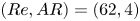$(Re,AR)=(62,4)$, mode $A$ is far above its threshold, which jeopardizes the use of the linear and weakly nonlinear stability tools. Further considerations about the effect of the second steady mode $C$ are provided in appendix B, while hereinafter we will focus on global modes $A$ and $B$ and their global interactions.

Figure 4. (a) Eigenvalues displayed in the $(\sigma ,\omega )$ plane for $Re=Re_{C_2}=22.65$ and $AR=AR_{C_2}=6.98$. A pair of complex eigenvalues, denoted by $B$ together with a pure real eigenvalue, $A$, are found to be simultaneously marginally stable for the present combination of parameters. Eigenvalues on the left side of the spectrum are not physical and correspond to spurious modes, whose presence is due to the influence of outlet boundary conditions. The position of eigenvalues $A$, $B$ and $C$ is not affected by $L_{out}$ in the range $L_{out}\in [30,100]$. (b) Marginal stability curves corresponding to the modes $A$ and $B$ and to a second steady mode $C$ as a function of $Re$ and $AR$. A codimension-2 point, $C_2$, is found for $Re=Re_{C_2}=22.65$ and $AR=AR_{C_2}=6.98$.

As a side remark to figure 4(b), an extrapolation of the marginal stability curve associated to mode $C$ suggests that it would cross the curve of mode $A$ for $Re>100$. Nevertheless, the eigenvalue calculation performed in the range $Re\in [100,230]$ (not visible in 4b) showed that, for $Re=230$ and $AR=1.75$, the stability boundary is still delimited by mode $A$ ($C$ does not cross $A$). Indeed the two curves for modes $A$ and $C$ seem to approach two asymptotes (as well as the curve for mode $B$), whose actual existence could be confirmed by higher Reynolds calculations, which are however beyond the scope of this work.

The symmetry properties which characterized the two global modes $A$ and $B$, reading

(4.12)\begin{gather} u_1^A(x,y)={-}u_1^A(x,-y)={-}u_1^A({-}x,y),\quad v_1^A(x,y)=v_1^A(x,-y)=v_1^A({-}x,y), \end{gather}

(4.13)\begin{gather}u_1^B(x,y)={-}u_1^B(x,-y)=u_1^B({-}x,y), \quad v_1^B(x,y)=v_1^B(x,-y)={-}v_1^B({-}x,y), \end{gather}

lead to the following axis boundary conditions:

(4.14)\begin{gather} u_1^{A}|_{\partial\varOmega_{h}}=0,\quad \left.\frac{\partial v_1^{A}}{\partial y}\right|_{\partial\varOmega_{h}}=0,\qquad u_1^{A}|_{\partial\varOmega_{v}}=0,\quad \left.\frac{\partial v_1^{A}}{\partial x}\right|_{\partial\varOmega_{v}}=0, \end{gather}

(4.15)\begin{gather}u_1^{B}|_{\partial\varOmega_{h}}=0,\quad \left.\frac{\partial v_1^{B}}{\partial y}\right|_{\partial\varOmega_{h}}=0,\qquad v_1^{B}|_{\partial\varOmega_{v}}=0,\quad \left.\frac{\partial u_1^{B}}{\partial x}\right|_{\partial\varOmega_{v}}=0. \end{gather}

For a given global mode, $\hat {\boldsymbol {q}}_1$, we also compute the corresponding adjoint global mode, $\hat {\boldsymbol {q}}_1^{{\dagger}ger }$, which will be used in § 5 and which satisfies the adjoint eigenvalue problem,

(4.16)\begin{equation} [(\sigma-\text{i}\omega)\mathcal{B}^{{{\dagger}ger}}+\mathcal{A}^{{{\dagger}ger}}] \hat{\boldsymbol{q}}_1^{{{\dagger}ger}}=\boldsymbol{0}, \end{equation}

where $\mathcal {A}^{{\dagger}ger }$ and $\mathcal {B}^{{\dagger}ger }$ are the adjoint operators of the linear operator $\mathcal {A}$ and the mass matrix $\mathcal {B}$, obtained by integrating by parts system (4.6) and expressed as

(4.17)\begin{equation} \mathcal{A}^{{{\dagger}ger}} = \begin{pmatrix} \mathcal{C}_{\textit{AR}}^{{{\dagger}ger}}(\boldsymbol{u}_0,\, \boldsymbol{\cdot} )-\dfrac{1}{Re}\varDelta_{\textit{AR}} & -\boldsymbol{\nabla}_{\textit{AR}}\\ \boldsymbol{\nabla}_{\textit{AR}}^{\textrm{T}} & 0 \end{pmatrix},\quad \mathcal{B}^{{{\dagger}ger}} = \begin{pmatrix} \mathcal{I} & 0 \\ 0 & 0 \end{pmatrix}. \end{equation}

Here $\mathcal {C}_{\textit {AR}}^{{\dagger}ger }(\boldsymbol {a},\boldsymbol {b})$ is the adjoint advection operator, which is not symmetric and which reads as $\mathcal {C}_{\textit {AR}}^{{\dagger}ger }(\boldsymbol {a},\boldsymbol {b})=-(\boldsymbol {a}\boldsymbol {\cdot }\boldsymbol {\nabla }_{\textit {AR}})^{\textrm {T}}\boldsymbol {b}+(\boldsymbol {b}\boldsymbol {\cdot }\boldsymbol {\nabla }_{\textit {AR}})\boldsymbol {a}$. The adjoint boundary conditions are defined so that all boundary terms arising from the integration by parts are nil. Thus, we obtain

(4.18)\begin{gather} \boldsymbol{u}_1^{{{\dagger}ger}}|_{\partial\varOmega_w}=\boldsymbol{0},\quad (\boldsymbol{u}_0\boldsymbol{\cdot}\boldsymbol{n})\hat{\boldsymbol{u}}_1^{{{\dagger}ger}} +\left.\left(p_1^{{{\dagger}ger}}\boldsymbol{I}+\frac{1}{Re}\nabla\boldsymbol{u}_1^{{{\dagger}ger}}\right) \boldsymbol{\cdot} \boldsymbol{n}\right|_{\partial\varOmega_o}=0,\quad \boldsymbol{u}_1^{{{\dagger}ger}}|_{\partial\varOmega_i}=\boldsymbol{0}, \end{gather}

(4.19)\begin{gather}u_1^{A{\dagger}ger}|_{\partial\varOmega_{h}}=0,\quad \left.\frac{\partial v_1^{A{\dagger}ger}}{\partial y}\right|_{\partial\varOmega_{h}}=0,\qquad u_1^{A{\dagger}ger}|_{\partial\varOmega_{v}}=0,\quad \left.\frac{\partial v_1^{A{\dagger}ger}}{\partial x}\right|_{\partial\varOmega_{v}}=0, \end{gather}

(4.20)\begin{gather}u_1^{B{\dagger}ger}|_{\partial\varOmega_{h}}=0,\quad \left.\frac{\partial v_1^{B{\dagger}ger}}{\partial y}\right|_{\partial\varOmega_{h}}=0,\qquad v_1^{B{\dagger}ger}|_{\partial\varOmega_{v}}=0,\quad \left.\frac{\partial u_1^{B{\dagger}ger}}{\partial x}\right|_{\partial\varOmega_{v}}=0. \end{gather}

We checked a posteriori that both direct and adjoint problems have an identical spectrum and the direct and adjoint modes satisfy the bi-orthogonality property (see Meliga et al. Reference Meliga, Chomaz and Sipp2009a).

Figures 5 and 6 show the spatial structure of the velocity fields along the $x$- and $y$-axis associated with the direct and adjoint global modes $A$ and $B$, respectively. While the direct modes are normalized using the value of the $y$-velocity field, $\hat {v}_1$, in a generic grid point, i.e. $(x,y)=(0.5,0)$, the adjoint modes are normalized such that $\langle \hat {\boldsymbol {q}}_1^{{\dagger}ger },\mathcal {B}\hat {\boldsymbol {q}}_1\rangle =1$, where $\langle \,,\rangle$ is the inner product defined by $\langle \boldsymbol {a},\boldsymbol {b}\rangle =\int _{\varOmega }\boldsymbol {a}^* \boldsymbol {\cdot }\boldsymbol {b}\,\textrm {d}\varOmega$, the star $^*$ denotes the complex conjugate and $\boldsymbol {\cdot }$ indicates the canonical Hermitian scalar product in $\mathbb {C}^n$. This normalization will simplify the expression of the various coefficients derived in § 5. In figure 5(b,d) the real part velocity components of the oscillating mode along the $x$- and $y$-axis are represented. Their spatial structure is qualitatively analogous to that recently presented in the 3-D study performed by Bertsch et al. (Reference Bertsch, Bongarzone, Duchamp, Renaud and Gallaire2020a), which confirms that this kind of instability arises in both 2-D and 3-D problems for proper combinations of control parameters, $Re$ and $AR$, and which suggests that the same physical mechanism is behind the origin of the self-sustained oscillations regime. As mentioned by Bertsch et al. (Reference Bertsch, Bongarzone, Duchamp, Renaud and Gallaire2020a), the structure of the perturbation velocity fields of mode $B$ in the left and right output channels and their well-defined wavelength is typical of sinuous shear instabilities, like the famous one characterizing the unsteady flow past a circular cylinder (Ding & Kawahara Reference Ding and Kawahara1999; Barkley Reference Barkley2006; Sipp & Lebedev Reference Sipp and Lebedev2007). From the analysis of the corresponding adjoint mode (see figure 6b,d), we see that the spatial structure of the adjoint is localized in the central region, near the two inlets. In classic shear instabilities of open flow, a downstream localization of the global mode and an upstream localization of the adjoint global mode resulting from the convective non-normality of the linearized Navier–Stokes operator (Chomaz Reference Chomaz2005) is observed. Identifying two downstream directions towards the outlets and two upstream directions corresponding to the inlets, a similar characteristic is found. This evidence motivates the detailed investigation, presented in § 7, of the nature of this instability, which, from the knowledge of the authors, remained undetermined so far.

Figure 5. Spatial structure of the $x$- and $y$-velocity components associated with the direct global modes $A$ and $B$ at the codimension-2 point, $C_2=(Re_{C_2},AR_{C_2})=(22.65,6.98)$. (a,c) Plots of the $x$- and $y$-velocity fields corresponding to the direct steady mode $A$. (b,d) Real part of the $x$- and $y$-velocity fields corresponding to the direct oscillating mode $B$.

Figure 6. Spatial structure of the $x$- and $y$-velocity components associated with the direct and adjoint global modes at the codimension-2 point, $C_2=(Re_{C_2},AR_{C_2})=(22.65,6.98)$. (a,c) Plots of the $x$- and $y$-velocity fields corresponding to the adjoint steady mode $A$. (b,d) Real part of the $x$- and $y$-velocity fields corresponding to the adjoint oscillating mode $B$.

Concerning the steady global mode $A$ (see figure 5a,c), it represents a steady symmetry-breaking condition with respect to the $x$-axis of symmetry. Given the symmetries of mode $A$, this steady instability corresponds to two possible new steady configurations (bi-stability), symmetric with respect to the $x$-axis. It leads to a positive off-set of the stagnation point above the $x$-axis (respectively a negative off-set below the $x$-axis) in the $y$-direction (at $x=0$); the two recirculation regions above (respectively below) the axis become smaller than the two below (respectively above) the axis. The corresponding adjoint mode (see figure 6a,c) maintains a structure similar to that of the direct mode.

The existence of a steady symmetry-breaking global mode and an oscillating global mode, which can be unstable in different regions of a stability map is also qualitatively consistent with the numerical analysis proposed by Pawlowski et al. (Reference Pawlowski, Salinger, Shadid and Mountziaris2006), who examined the same 2-D configuration with the only difference that a plug inlet profile was considered (see § 8 for further comments about the influence of a plug inlet velocity profile).

5.1. Presentation

Since a codimension-2 point, $C_2=(Re_{C_2},AR_{C_2})=(22.65,6.98)$, is found from the linear stability analysis, we present in this section a WNL in order to investigate the mode interaction between the steady mode $A$ and the oscillating mode $B$. In other words, we implement an asymptotic expansion where the two modes have the same order of magnitude. The departure from criticality, in terms of Reynolds number and aspect ratio, is assumed to be of order $\epsilon ^2$. Hence, we introduce the two order one parameters, $\delta =\epsilon ^2\tilde {\delta }$ and $\alpha =\epsilon ^2\tilde {\alpha }$, such that

(5.1)\begin{equation} \frac{1}{Re}=\frac{1}{Re_{C_2}}-\epsilon^2\tilde{\delta},\quad \frac{1}{AR}=\frac{1}{AR_{C_2}}+\epsilon^2\tilde{\alpha}. \end{equation}

In the spirit of the multiple scale technique, we introduce the slow time scale $T=\epsilon ^2 t$, with $t$ being the fast time scale defined in (2.1). Hence, the entire flow field is expanded as

(5.2)\begin{equation} \boldsymbol{q}=\{u,v,p\}^{\textrm{T}}=\boldsymbol{q}_0+\epsilon\boldsymbol{q}_1+\epsilon^2\boldsymbol{q}_2+\epsilon^3\boldsymbol{q}_3+\text{O}(\epsilon^4). \end{equation}

In order to easily write the equations at the various order in $\epsilon$ in a compact form, it is useful to introduce the following expansion for the nabla operator, $\boldsymbol {\nabla }$:

(5.3)\begin{align} \boldsymbol{\nabla}_{\textit{AR}}&=\left\{\frac{\partial}{\partial x},\frac{1}{AR}\frac{\partial}{\partial y}\right\}^{\textrm{T}}=\left\{\frac{\partial}{\partial x},\frac{1}{AR_{C_2}}\frac{\partial}{\partial y}\right\}^{\textrm{T}}+\epsilon^2\tilde{\alpha}\left\{0,\frac{\partial}{\partial y}\right\}^{\textrm{T}}\nonumber\\ &=\boldsymbol{\nabla}_{AR_{C_2}}+\epsilon^2\tilde{\alpha}\boldsymbol{\nabla}_{\alpha}+\text{O}(\epsilon^3). \end{align}

The definition of the Laplacian follows as

(5.4)\begin{align} \varDelta_{\textit{AR}}&=\boldsymbol{\nabla}_{\textit{AR}}^{\textrm{T}}\boldsymbol{\nabla}_{\textit{AR}}=(\boldsymbol{\nabla}_{AR_{C_2}}+\epsilon^2\tilde{\alpha}\boldsymbol{\nabla}_{\alpha})^{\textrm{T}}(\boldsymbol{\nabla}_{AR_{C_2}}+\epsilon^2\tilde{\alpha}\boldsymbol{\nabla}_{\alpha})\nonumber\\ &=\left(\frac{\partial^2}{\partial x^2}+\frac{1}{AR_{C_2}^2} \frac{\partial^2}{\partial y^2}\right)+\epsilon^2 \frac{2\tilde{\alpha}}{AR_{C_2}} \frac{\partial^2}{\partial y^2}=\varDelta_{AR_{C_2}}+\epsilon^2 2 \tilde{\alpha} \varDelta_{\alpha AR_{C_2}}+\text{O}(\epsilon^3). \end{align}

Substituting the expansions defined above in the governing equations (2.2) and (2.3) with their boundary conditions, a series of problems at the different orders in $\epsilon$ are obtained.

5.2. Order $\epsilon ^0$: steady base flow

At order $\epsilon ^0$ the system is represented by the nonlinear equations for the steady symmetric base flow (4.1) with boundary conditions (4.2)–(4.5). The solution, computed for $Re_{C_2}$ and $AR_{C_2}$ via iterative Newton's method, was described in § 4.1.

5.3. Order $\epsilon$: linear global stability

At leading order in $\epsilon$ the system is represented by the unsteady Navier–Stokes equations linearized around the base flow for $Re_{C_2}$ and $AR_{C_2}$, whose solution has been presented in § 4.2. In this framework, the solution of the leading order system is assumed to be composed of the sum of the two global modes, $A$ and $B$,

(5.5)\begin{equation} \boldsymbol{q}_1=A(T)\hat{\boldsymbol{q}}_1^A+(B(T)\hat{\boldsymbol{q}}_1^B\,\textrm{e}^{\text{i}\omega t}+\text{c.c.}), \end{equation}

that destabilized the steady state $\boldsymbol {q}_0$. In (5.5) the amplitude $A(T)$, which varies with the slow time scale $T$, and the associated normalized eigenfunction are purely real, while the amplitude $B(T)$ and eigenfunction for mode $B$ are complex. Introducing (5.5) in the $\epsilon$-order system, a generalized eigenvalue problem for mode $A$ and $B$, whose general form reads as $(\text {i}\omega \mathcal {B}+\mathcal {A})\hat {\boldsymbol {q}}_1=\boldsymbol {0}$, is retrieved. We remark that at the codimension-2 point both modes are marginally stable, therefore, their growth rates are nil, $\sigma _A=\sigma _B=0$ in $C_2$, while the oscillation frequency of mode $B$ is $\omega =0.10157$.

5.4. Order $\epsilon ^2$: base-flow modifications, mean-flow corrections, mode interaction and second-harmonic response

At order $\epsilon ^2$ we obtain the linearized Navier–Stokes equations applied to $\boldsymbol {q}_2=\{\boldsymbol {u}_2,p_2\}^{\textrm {T}}$,

(5.6)\begin{equation} (\mathcal{B}\partial_t+\mathcal{A})\boldsymbol{q}_2=\boldsymbol{\mathcal{F}}_2, \end{equation}

with the boundary conditions

(5.7)\begin{equation} \boldsymbol{u}_2|_{\partial\varOmega_w}=\boldsymbol{0},\ \ \left.\left({-}p_2\boldsymbol{I}+\frac{1}{Re_{C_2}}\boldsymbol{\nabla}_{AR_{C_2}}\boldsymbol{u}_2\right)\boldsymbol{\cdot}\boldsymbol{n}\right|_{\partial\varOmega_o}=0,\ \ \boldsymbol{u}_2|_{\partial\varOmega_i}=\boldsymbol{0}, \end{equation}

and forced by a term $\boldsymbol {\mathcal {F}}_2$ depending only on zero- and first-order solutions,

(5.8)\begin{align} \boldsymbol{\mathcal{F}}_2= \begin{pmatrix} -\tilde{\delta}\varDelta_{AR_{C_2}}\boldsymbol{u}_0+ \dfrac{2\tilde{\alpha}}{Re_{C_2}}\varDelta_{\alpha AR_{C_2}}\boldsymbol{u}_0-\tilde{\alpha}\boldsymbol{\nabla}_{\alpha}p_0- \dfrac{\tilde{\alpha}}{2}\mathcal{C}_{\alpha}(\boldsymbol{u}_0,\boldsymbol{u}_0) -\frac{1}{2}\mathcal{C}_{AR_{C_2}}(\boldsymbol{u}_1,\boldsymbol{u}_1)\\ -\tilde{\alpha}\boldsymbol{\nabla}_{\alpha}\cdot\boldsymbol{u}_0 \end{pmatrix}, \end{align}

where $\mathcal {C}_{\alpha }$ is the $\epsilon ^2$-order symmetric advection operator, $\mathcal {C}_{\alpha }(\boldsymbol {a},\boldsymbol {b})=(\boldsymbol {a}\boldsymbol {\cdot }\boldsymbol {\nabla }_{\alpha })\boldsymbol {b} +(\boldsymbol {b}\boldsymbol {\cdot }\boldsymbol {\nabla }_{\alpha })\boldsymbol {a}$, while $\mathcal {C}_{AR_{C_2}}(\boldsymbol {a},\boldsymbol {b})=(\boldsymbol {a}\boldsymbol {\cdot }\boldsymbol {\nabla }_{AR_{C_2}}) \boldsymbol {b}+(\boldsymbol {b}\boldsymbol {\cdot }\boldsymbol {\nabla }_{AR_{C_2}})\boldsymbol {a}$. Terms proportional to $\delta$ and $\alpha$ arise from the Reynolds number and aspect ratio variations with respect to the codimension-2 point definition and they act on the base flow. The last term in the $y$-component of (5.8) is due to the transport of the first-order solution $\boldsymbol {q}_1$ by itself. Introducing the first-order normal form (5.5) in the forcing term expressed in (5.8), the different contributions can be individualized to give

(5.9)\begin{equation} \boldsymbol{\mathcal{F}}_2=\underbrace{\tilde{\delta}\widehat{\boldsymbol{\mathcal{F}}}_2^{\delta} +\tilde{\alpha}\widehat{\boldsymbol{\mathcal{F}}}_2^{\alpha}+A^2\widehat{\boldsymbol{\mathcal{F}}}_2^{A^2} +|B|^2\widehat{\boldsymbol{\mathcal{F}}}_2^{|B|^2}}_{\boldsymbol{\mathcal{F}}_2^j =\{\mathcal{F}_{2x}^j,\mathcal{F}_{2y}^j\}^{\textrm{T}}}+(B^2\widehat{\boldsymbol{\mathcal{F}}}_2^{B^2}\,\textrm{e}^{\text{i}2\omega t}+AB\widehat{\boldsymbol{\mathcal{F}}}_2^{AB}\,\textrm{e}^{\text{i}\omega t}+\text{c.c.}). \end{equation}

Looking at (5.9), we recognize the second harmonic for mode $B$, which is pulsating at $2\omega \ne \omega$ and, thus, it does not resonate and does not need the imposition of any compatibility condition. In principle, all the other terms could be classified as resonating terms in mode $A$ or $B$ for which the forced problem results to be singular and, hence, it is necessary to verify the solvability condition or Fredholm alternative. However, we can make use of the symmetry properties of the various forcing terms, as recently proposed in Camarri & Mengali (Reference Camarri and Mengali2019), to show that some of these conditions are implicitly satisfied. Indeed, the first four forcing terms, having $\omega =0$, are characterized by the symmetries at the $x$- and $y$-axis, i.e.

(5.10)\begin{equation} \mathcal{F}_{2y}^{j}|_{\partial\varOmega_{h}}=0,\quad \left.\frac{\partial \mathcal{F}_{2x}^{j}}{\partial y}\right|_{\partial\varOmega_{h}}=0,\qquad \mathcal{F}_{2x}^{j}|_{\partial\varOmega_{v}}=0,\quad \left.\frac{\partial \mathcal{F}_{2y}^{j}}{\partial x}\right|_{\partial\varOmega_{v}}=0, \end{equation}

which does not coincide with the axis boundary conditions for mode $A$ given in (4.14). Consequently, the solvability condition for $A$ is naturally satisfied by symmetry properties. The same argument is applicable to the last terms oscillating in $\omega$, arising from direct competition between modes $A$ and $B$, which is characterized by the symmetries

(5.11)\begin{equation} \hat{\mathcal{F}}_{2y}^{AB}|_{\partial\varOmega_{h}}=0,\quad \left.\frac{\partial \hat{\mathcal{F}}_{2x}^{AB}}{\partial y}\right|_{\partial\varOmega_{h}}=0,\qquad \hat{\mathcal{F}}_{2y}^{AB}|_{\partial\varOmega_{v}}=0,\quad \left.\frac{\partial \hat{\mathcal{F}}_{2x}^{AB}}{\partial x}\right|_{\partial\varOmega_{v}}=0, \end{equation}

that differ from the boundary conditions for mode $B$ given in (4.15) and automatically satisfy the solvability condition. It follows that, using the mentioned symmetry considerations, no solvability condition needs to be imposed at the $\epsilon ^2$-order. We thus look for a second-order solution having the expression

(5.12)\begin{equation} \boldsymbol{q}_2=\tilde{\delta}\hat{\boldsymbol{q}}_2^{\delta}+\tilde{\alpha}\hat{\boldsymbol{q}}_2^{\alpha} +A^2\hat{\boldsymbol{q}}_2^{A^2}+|B|^2\hat{\boldsymbol{q}}_2^{|B|^2} +(B^2\hat{\boldsymbol{q}}_2^{B^2}\,\textrm{e}^{\text{i}2\omega t}+AB\hat{\boldsymbol{q}}_2^{AB}\,\textrm{e}^{\text{i}\omega t}+\text{c.c.}), \end{equation}

where each single response is evaluated by means of a global resolvent technique (Garnaud et al. Reference Garnaud, Lesshafft, Schmid and Huerre2013; Viola, Arratia & Gallaire Reference Viola, Arratia and Gallaire2016).

All the second-order responses are displayed in figure 7 in terms of their $x$-velocity component. As shown in figure 7(f), the second-harmonic response for the global mode $B$ is essentially periodic in space with a wavelength twice that of the direct mode (see figure 5b,d), while the interaction between $A$ and $B$ (see figure 7e) is nearly periodic in space with a wavelength close to that of the direct mode $B$ within a central region near the jets collision, where the direct mode $A$ mainly acts, and it vanishes far away as mode $A$ vanishes too (see figure 5a,c).

Figure 7. Second-order responses corresponding respectively to (a,b) base-flow modifications due to the Reynolds number and aspect ratio variations with respect to the codimension-2 point, $C_2$, (c,d) mean-flow correction associated to mode $A$ and $B$, respectively, (e,f) harmonic interaction between the steady mode $A$ and the oscillating mode $B$ and second harmonic for mode $B$.

5.5. Order $\epsilon ^3$: amplitude equations

At the $\epsilon ^3$-order we derive the system of amplitude equations which describe the weakly nonlinear global mode interaction of $A$ and $B$. The problem at order $\epsilon ^3$ is similar to the one obtained at order $\epsilon ^2$, as it indeed appears as a linear system forced by the previous order solutions, englobed in $\mathcal {F}_3$,

(5.13)\begin{equation} (\mathcal{B}\partial_t+\mathcal{A})\boldsymbol{q}_3=\boldsymbol{\mathcal{F}}_3, \end{equation}

and subjected to the boundary conditions,

(5.14)\begin{equation} \boldsymbol{u}_3|_{\partial\varOmega_w}=\boldsymbol{0},\quad \left.\left({-}p_3\boldsymbol{I}+\frac{1}{Re_{C_2}}\boldsymbol{\nabla}_{AR_{C_2}}\boldsymbol{u}_3\right) \boldsymbol{\cdot}\boldsymbol{n}\right|_{\partial\varOmega_o}=0,\quad \boldsymbol{u}_3|_{\partial\varOmega_i}=\boldsymbol{0}. \end{equation}

The $\epsilon ^3$-order forcing term, $\boldsymbol {\mathcal {F}}_3$, by substituting the first- and second-order solutions, reads as

(5.15) \begin{align} & \boldsymbol{\mathcal{F}}_3\notag\\ & \quad =\begin{pmatrix} -\partial_T\boldsymbol{u}_1-\tilde{\delta}\varDelta_{AR_{C_2}}\boldsymbol{u}_1 +\dfrac{2\tilde{\alpha}}{Re_{C_2}}\varDelta_{\alpha AR_{C_2}}\boldsymbol{u}_1-\tilde{\alpha}\boldsymbol{\nabla}_{\alpha}p_1- \tilde{\alpha}\mathcal{C}_{\alpha}(\boldsymbol{u}_0,\boldsymbol{u}_1) -\mathcal{C}_{AR_{C_2}}(\boldsymbol{u}_1,\boldsymbol{u}_2)\\ -\tilde{\alpha}\boldsymbol{\nabla}_{\alpha}\boldsymbol{u}_1 \end{pmatrix}\nonumber\\ & \quad ={-}\frac{\partial A}{\partial T}{\mathcal{B}} \hat{\boldsymbol{q}}_1^A+A(\tilde{\delta}\widehat{\boldsymbol{\mathcal{F}}}_3^{\delta A}+\tilde{\alpha}\widehat{\boldsymbol{\mathcal{F}}}_3^{\alpha A})+A^3\widehat{\boldsymbol{\mathcal{F}}}_3^{A^3}+A|B|^2\widehat{\boldsymbol{\mathcal{F}}}_3^{A|B|^2}\notag\\ & \qquad +\left\{\left[-\frac{\partial B}{\partial T}\mathcal{B}\hat{\boldsymbol{q}}_1^B+B(\tilde{\delta}\widehat{\boldsymbol{\mathcal{F}}}_3^{\delta B}+\tilde{\alpha}\widehat{\boldsymbol{\mathcal{F}}}_3^{\alpha B})+|B|^2B\widehat{\boldsymbol{\mathcal{F}}}_3^{|B|^2B}+A^2B\widehat{\boldsymbol{\mathcal{F}}}_3^{A^2B}\right]\textrm{e}^{\text{i}\omega t}+\text{c.c.}\right\}\nonumber\\ &\qquad +\text{N.R.T.}, \end{align}

where $\text {N.R.T.}$ gathers all the non-resonating terms, not relevant for the further analysis and omitted thereafter. The first term in the $y$-component of (5.15) corresponds to the slow time evolution of the amplitudes $A(T)$ and $B(T)$ with the slow time scale $T=\epsilon ^2t$. The last term is due to the advection of the leading order solution by the second-order solution and vice versa. All the other terms arise from the Reynolds number and aspect ratio variation acting on the $\epsilon$-order solution. As standard in multiple scale analysis, in order to avoid secular terms and solve the expansion procedure at the third order, a compatibility condition must be enforced through the Fredholm alternative (Friedrichs Reference Friedrichs2012).

The compatibility condition imposes the amplitudes $A(T)$ and $B(T)$ to obey the relations

(5.16)\begin{align} \frac{\textrm{d}A}{\textrm{d}t}=(\delta\zeta_A+\alpha\eta_A)A-\mu_AA^3-\chi_AA|B|^2, \end{align}

(5.17)\begin{align} \frac{\textrm{d}B}{\textrm{d}t}=(\delta\zeta_B+\alpha\eta_B)B-\mu_B|B|^2B-\chi_BBA^2, \end{align}

where the physical time scale $t$ has been reintroduced, $\delta =\epsilon ^2\tilde {\delta }=1/Re_{C_2}-1/Re$, $\alpha =\epsilon ^2\tilde {\alpha }=1/AR-1/AR_{C_2}$ and the various coefficients, whose values are reported in appendix A, are computed as scalar products between the adjoint global modes $\hat {\boldsymbol {q}}_1^{{\dagger}ger }$ and the resonant forcing terms $\widehat {\boldsymbol {\mathcal {F}}}_3^i$, i.e. for instance,

(5.18)\begin{equation} \zeta_A=\frac{\langle \hat{\boldsymbol{q}}_1^{A{\dagger}ger},\widehat{\boldsymbol{\mathcal{F}}}_3^{\delta A}\rangle}{\langle \hat{\boldsymbol{q}}_1^{A{\dagger}ger},\mathcal{B}\hat{\boldsymbol{q}}_1^{A}\rangle } =\langle \hat{\boldsymbol{q}}_1^{A{\dagger}ger},\widehat{\boldsymbol{\mathcal{F}}}_3^{\delta A}\rangle ,\quad \zeta_B=\frac{\langle \hat{\boldsymbol{q}}_1^{B{\dagger}ger},\widehat{\boldsymbol{\mathcal{F}}}_3^{\delta B}\rangle }{\langle \hat{\boldsymbol{q}}_1^{B{\dagger}ger},\mathcal{B}\hat{\boldsymbol{q}}_1^{B}\rangle } =\langle \hat{\boldsymbol{q}}_1^{B{\dagger}ger},\widehat{\boldsymbol{\mathcal{F}}}_3^{\delta B}\rangle , \end{equation}

since $\langle \hat {\boldsymbol {q}}_1^{A{\dagger}ger },\mathcal {B}\hat {\boldsymbol {q}}_1^{A}\rangle =\langle \hat {\boldsymbol {q}}_1^{B{\dagger}ger },\mathcal {B}\hat {\boldsymbol {q}}_1^{B}\rangle =1$ due to the normalization introduced in § 4.2. The detailed expression of each normal form coefficient is provided in appendix A. Equations (5.16) and (5.17) differ from the classic Stuart–Landau equations, describing the pitchfork and Hopf bifurcations of single modes, by the two coupling terms, $\chi _AA|B|^2$ and $\chi _BBA^2$, coming from third-order nonlinearities. The structure of system (5.16) and (5.17) is well known in literature and is analogous to that derived by Meliga et al. (Reference Meliga, Gallaire and Chomaz2012), where a formally equivalent analysis is performed to investigate weakly nonlinear interactions for mode selection in swirling jets.

5.5.1. Stability analysis of the amplitude equations

Here we perform the stability analysis of the amplitude (5.16) and (5.17). Recalling that the amplitude $A$ is purely real, as well as all the coefficients associated with its equation, while amplitude $B$ and the related amplitude equation coefficients are complex, so that we can turn to polar coordinates, i.e. $B=|B|\,\textrm {e}^{\text {i}\varPhi _B}$, and split the modulus and phase parts of (5.16) and (5.17),

(5.19)\begin{align} \frac{\textrm{d}A}{\textrm{d}t}=(\delta\zeta_A+\alpha\eta_A)A-\mu_AA^3-\chi_AA|B|^2, \end{align}

(5.20)\begin{align} \frac{\textrm{d}|B|}{\textrm{d}t}=(\delta\zeta_{Br}+\alpha\eta_{Br})|B|-\mu_{Br}|B|^3-\chi_{Br}|B|A^2, \end{align}

(5.21)\begin{align} \frac{\textrm{d}\varPhi_B}{\textrm{d}t}=(\delta\zeta_{Bi}+\alpha\eta_{Bi})-\mu_{Bi}|B|^2-\chi_{Bi}A^2. \end{align}

System (5.19) and (5.20) presents different possible equilibria (Kuznetsov Reference Kuznetsov2013). Below the threshold the system is stable and the trivial equilibrium with $A=|B|=0$ is retrieved. Two other possible equilibria correspond to $(A\ne 0,|B|=0)$ (pitchfork bifurcation for mode $A$) or $(A=0,|B|\ne 0)$ (Hopf bifurcation for mode $B$). The single mode pitchfork and Hopf bifurcations are easily found, removing the coupling terms by setting $\chi _A=\chi _B=0$ and looking for a stationary solution of (5.19) and (5.20), ${\textrm {d}A}/{\textrm {d}t}={\textrm {d}|B|}/{\textrm {d}t}=0$. This leads to the classic solutions

(5.22)\begin{equation} A^2=\frac{\delta\zeta_A+\alpha\eta_A}{\mu_A},\quad |B|^2=\frac{\delta\zeta_{Br}+\alpha\eta_{Br}}{\mu_{Br}}. \end{equation}

The non-trivial equilibrium with $(A\ne 0,|B|\ne 0)$ is obtained reintroducing the coupling terms and investigating the existence of a parameter region in which both modes coexist. Indeed, looking for a stationary solution ${\textrm {d}A}/{\textrm {d}t}={\textrm {d}|B|}/{\textrm {d}t}=0$, we obtain the system

(5.23)\begin{equation} \left[ \begin{matrix} \mu_A & \chi_A \\ \chi_{Br} & \mu_{Br} \end{matrix} \right] \left\{ \begin{matrix} A^2 \\ |B|^2 \end{matrix} \right\}= \left\{ \begin{matrix} \delta\zeta_{A}+\alpha\eta_{A} \\ \delta\zeta_{Br}+\alpha\eta_{Br} \end{matrix} \right\}, \end{equation}

which admits a physical solution only for $Re$ and $AR$ values for which $A^2>0$ and $|B|^2>0$. Solving (5.23), we obtain

(5.24)\begin{align} A^2&=\frac{(\delta\zeta_A+\alpha\eta_A)\mu_{B_r}-\chi_A(\delta\zeta_{B_r} +\alpha\eta_{B_r})}{\mu_A\mu_{B_r}-\chi_A\chi_{B_r}}, \end{align}

(5.25)\begin{align} |B|^2&=\frac{(\delta\zeta_{B_r}+\alpha\eta_{B_r})\mu_A-\chi_{B_r}(\delta\zeta_A+\alpha\eta_A)}{\mu_A\mu_{B_r}-\chi_A\chi_{B_r}}. \end{align}

The general relation for the phase of mode $B$ at large time, which varies linearly in time, reads as

(5.26)\begin{equation} \varPhi_B|_{t\rightarrow +\infty}=[(\delta\zeta_{Bi}+\alpha\eta_{Bi})-\mu_{Bi}|B|^2-\chi_{Bi}A^2]t, \end{equation}

meaning that the frequency at large time will saturate to the following prescribed valued, function of the Reynolds number and aspect ratio variation with respect to the codimension-2 point, $C_2$:

(5.27)\begin{equation} \omega|_{t\rightarrow +\infty}=\omega_{C_2}+[(\delta\zeta_{Bi}+\alpha\eta_{Bi})-\mu_{Bi}|B|^2-\chi_{Bi}A^2]. \end{equation}

Combining all these ingredients, the bifurcation diagram proposed in figure 8(a–c) presents a complex series of bifurcations. The stability of the various branches was numerically assessed by time marching (5.19) and (5.20) using the Matlab function ode23. As depicted in figure 8(b) for a fixed value of aspect ratio, $AR=6.5<AR_{C_2}$, the steady mode $A$ bifurcates first at 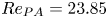$Re_{PA}=23.85$ (pitchfork bifurcation $\text {PA}$) breaking the symmetry of the base flow with respect to the $x$-axis, $\partial \varOmega _h$. The oscillating mode $B$ then bifurcates from the $x$-symmetry-breaking pitchfork bifurcation at 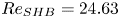$Re_{SHB}=24.63$ through a secondary Hopf bifurcation (SHB). Notwithstanding the subcritical nature of this bifurcation, which makes it unstable, such a bifurcated branch is fundamental for the emergence of the self-sustained oscillation regime, through a backward bifurcation of mode $A$ (BA) at 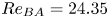$Re_{BA}=24.35$. The sub-criticality of the system in the range 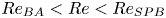$Re_{BA}<Re<Re_{SPB}$ leads to an hysteretic behaviour where either the steady mode $A$ or the oscillating mode $B$ can dominate, depending on the initial conditions to which the system is subjected. Figure 8(a) shows the full weakly nonlinear map predicted by the normal form (5.16) and (5.17) in the $(Re,AR)$-plane around the codimension-2 point. Lastly, as shown in figure 8(c), above $AR_{C_2}$ only the oscillating mode $B$, which settles into a limit cycle via classic Hopf bifurcation (HB), exists. In this range, the self-sustained oscillations regime is observed above a certain Reynolds number.

Figure 8. (a) Weakly nonlinear map predicted by the normal form (5.16) and (5.17) in the $(Re,AR)$-plane. Green and blue dotted lines indicate the linear marginal stability curves for mode $A$ and $B$, respectively, as presented in § 4.2. In the black region the steady mode $A$ prevails, while the oscillating mode $B$ dominates in the wide grey region. A region of hysteresis, highlighted in a light grey shade, is found for $AR$ smaller than $AR_{C_2}$. (b) Bifurcation diagram as a function of the Reynolds number for a fixed value of aspect ratio, $AR=6.5<AR_{C_2}$. Dashed and dot–dashed lines mean unstable branches, while solid lines denote stable branches. The vertical red dotted lines represent the thresholds for the pitchfork bifurcation of mode $A$ (PA), the backward bifurcation of mode $A$ (BA) and the secondary Hopf bifurcation of mode $B$ (SHB). The light grey shaded region corresponds to the hysteresis range of (a). (c) Bifurcation diagram as a function of the Reynolds number for a fixed value of aspect ratio, 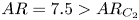$AR=7.5>AR_{C_2}$. The vertical red dotted lines represent the thresholds for the Hopf bifurcation for mode $B$.

6.1. Regime comparison

In figure 9 the nonlinear map of figure 8(a) for a specific value of aspect ratio in the region characterized by the hysteretic behaviour, i.e. $AR=6.5$, is recalled. Different DNS, covering the range of Reynolds numbers from the stable region (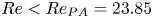$Re<Re_{PA}=23.85$) to the region dominated by the oscillating mode $B$ (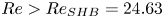$Re>Re_{SHB}=24.63$) were performed. The investigated cases are indicated in figure 9 with symbols. The results extracted from the DNS are presented in figures 10 and 11.

Figure 9. Nonlinear map of figure 8(a) for a specific value of aspect ratio in the region characterized by the hysteretic behaviour, i.e. $AR=6.5$. Cases investigated by performing DNS are indicated by symbols. The red diamond ($Re=24.55$) corresponds to a case in which the existence of the hysteresis region has been checked using the same control parameters, $AR$ and $Re$, but different initial conditions, given by the final steady state or limit cycle of the two closest simulations, whose Reynolds numbers have been increased or decreased, respectively, as sketched by the green arrows.

Figure 10. Snapshots of the flow patterns in terms of dye concentrations observed at large time, (a–d) once the steady state (stable base flow or symmetry breaking for mode $A$) is reached or, alternatively, (e,f) once the limit cycle for mode $B$ is fully established, for the various Reynolds numbers indicated by white squares in figure 9. The white dashed lines represent the axes of symmetry characterizing the steady base flow. The flow configuration for $Re=24.55$ is shown in figure 11.

Figure 11. Snapshots of the flow patterns in terms of dye concentrations observed at large time for $AR=6.5$ and the same Reynolds number, $Re=24.55$ (hysteresis region), but with different initial conditions: (a) the new steady state (symmetry-breaking condition) obtained for $Re=24.4$ is used as an initial condition; (b) a time instant of the unsteady solution corresponding to $Re=24.7$ (limit cycle for mode $B$) is imposed as an initial condition. Streamlines and arrows are used to visualize the velocity fields associated with the steady and oscillating configurations, respectively.

All the numerical simulations displayed in figure 10 were started from zero initial conditions. Figure 10(a) shows the steady state obtained for $Re=22$, which confirms that the steady base flow is stable for $Re<Re_{PA}=23.85$, indeed no symmetry breaking can be observed. For $Re=24$, $24.2$ and $24.4$ (which lies in the hysteresis range), we retrieved that the steady mode $A$ first bifurcates via a pitchfork bifurcation. The symmetry with respect to the $x$-axis is lost, the position of the stagnation point lies below the $x$-axis of symmetry and the size of the recirculation regions differs on either side of the $x$-axis of symmetry $\partial \varOmega _h$. For $Re>Re_{SHB}=24.63$, i.e. $Re=24.7$, $24.84$, $25$ and $27$, only the self-sustained oscillation regime is observed.

In order to confirm the existence of the hysteretic behaviour found in § 5.5.1, the solutions obtained at large time for $Re=24.4$ (asymmetric steady configuration) and $Re=24.7$ (limit cycle for the self-oscillations) are used as initial conditions for two more simulations, where the Reynolds number is fixed to $Re=24.55$ in both cases (filled red diamond and green arrows in figure 9). The results of this numerical procedure are given in figure 11. We clearly see in figure 11(a,b) that depending on the initial conditions imposed on the system, for this fixed value of $Re=24.55$ within the hysteresis region, both modes can emerge. Other simulations (not shown) performed in the upper region of figure 8(a), i.e. for $Re=25$ and $AR=7.5$ and $8$, confirm the supercritical nature of the Hopf bifurcation associated to mode $B$ (HB).

Next, global linear stability and WNL are both compared with the DNS in terms of the amplitude of modes $A$ and $B$ and oscillation frequency for the self-sustained oscillatory regime.

6.2. Frequency comparison

Figure 12(a) shows that, near the threshold, the linear global stability analysis (LGS), the WNL and DNS agree well and prescribe the correct oscillation frequency. However, if the LGS soon diverges from the DNS, as extensively described in the literature (Barkley Reference Barkley2006), the WNL theory, applied to the problem presented in this paper provides a wider range of Reynolds numbers in which the model follows the DNS trend with a satisfactory agreement, showing an error of $3\,\%$ for $Re=40$ against the $13.2\,\%$ of the LGS. Additionally, it needs to be underlined that the results shown in this section refer to an aspect ratio of $AR=6.5$, hence, a double off-set (in terms of $Re$ and $AR$) with respect to the codimension-2 point, $C_2$, is considered in the WNL curve of figure 12. Indeed, the precision of the asymptotic expansion prediction increases as $|Re-Re_{C_2}|$ and $|AR-AR_{C_2}|$ decrease.

Figure 12. (a) Oscillation frequency, extracted from the $y$-velocity component at $(x,y)=(0.5,0)$, versus Reynolds number for $AR=6.5$. The solid black line indicates the WNL. The dotted black line and plus signs represent the LGS. The dashed black line and circles are associated with the DNS performed. (b) Amplitude of modes $A$ and $B$ extracted from DNS and compared with the bifurcation diagram obtained from the WNL analysis for $AR=6.5$. Symbols and green arrows in (b) correspond to those introduced in figure 9 and are associated to the DNS presented above.

6.3. Amplitude comparison

In figure 12(b) we compare the amplitude of modes $A$ and $B$ extracted from the DNS with those prescribed by the WNL model. The total flow solutions in the steady and oscillatory regimes evaluated via weakly nonlinear formulation read as

(6.2)\begin{equation} \boldsymbol{u}^A_{WNL}=\boldsymbol{u}_0+A\boldsymbol{u}_1^A+\delta\boldsymbol{u}_2^{\delta} +\alpha\boldsymbol{u}_{2}^{\alpha}+A^2\boldsymbol{u}_{2}^{A^2}, \end{equation}

(6.3)\begin{equation}\boldsymbol{u}^B_{WNL}=\boldsymbol{u}_0+(B\boldsymbol{u}_1^B\,\textrm{e}^{\text{i}\omega t}+\textrm{c.c.})+\delta\boldsymbol{u}_2^{\delta}+\alpha\boldsymbol{u}_{2}^{\alpha} +|B|^2\boldsymbol{u}_{2}^{|B|^2}+(B^2\boldsymbol{u}_2^{B^2}\,\textrm{e}^{\text{i}2\omega t}+\textrm{c.c.}). \end{equation}

Specifying (6.2) and (6.3) for the $y$-velocity components, $v_{WNL}^{A,B}$, at the $x$-axis of symmetry ($y=0$), given the symmetries of the various terms, we have $v^A(x,0)_{WNL}=Av_1^A(x,0)$ and $v^B(x,0)_{WNL}=(Bv_1^B(x,0)\,\textrm {e}^{\text {i}\omega t}+\textrm {c.c.})$. Then selecting the point $x=0.5$, used to normalize the global modes ($v_1^A(0,5,0)=1$ and $v_1^B(0.5,0)=1$), we derive the simple expressions

(6.4)\begin{equation} v^A(0.5,0)_{WNL}=A, \end{equation}

(6.5)\begin{equation}v^B(0.5,0)_{WNL}=2|B|\cos(\omega t+\varPhi_B), \end{equation}

which allow us to easily compare the amplitudes $A$ and $|B|$ from the WNL model with those extracted from the DNS, $v(0.5,0)_{DNS}$. Figure 12(b) shows not only a qualitative but also a quantitative agreement between DNS and WNL, which captures well the hysteretic behaviour of the flow for $AR<AR_{C_2}$ (sufficiently close to $AR_{C_2}$).

6.4. Evolution of the oscillation frequency with the aspect ratio

A linear dependence of the self-oscillations on the inverse of the spacing between the jets, $s$, which highlights the importance of the distance $s$ in the oscillatory phenomenon, was observed in Bertsch et al. (Reference Bertsch, Bongarzone, Duchamp, Renaud and Gallaire2020a), who proposed the scaling law

(6.6)\begin{equation} f\sim \frac{U}{s}, \end{equation}

where the slope, derived by fitting the experimental data, was seen to be approximatively $1/6$, which is also consistent with the measurements made by Denshchikov et al. (Reference Denshchikov, Kondrat'ev and Romashov1978) on large-scale facing jets in turbulent flow conditions. Given the definition of the Strouhal number introduced in § 4.2, $St=fw/U$, and the aspect ratio $AR=s/w$, the non-dimensional form of the scaling law (6.6) reads as

(6.7)\begin{equation} St_B\sim \frac{1}{AR}, \end{equation}

where the subscript $_B$ is used to denote the frequency associated with the oscillating mode $B$. It follows that in our 2-D model, (6.6) translates in a linear dependence of the Strouhal number on $1/AR$. Moreover, according to such a law, the variation of $St$ with $Re$ is not predominant.

In order to verify whether the evolution of the oscillation frequency in our 2-D flow behaves similarly to that of the 3-D one studied in Bertsch et al. (Reference Bertsch, Bongarzone, Duchamp, Renaud and Gallaire2020a), we performed a series of DNS fixing $Re$, i.e. $Re=Re_{C_2}=22.65$, and varying $AR$ ($>AR_{C_2}$). A quantitative comparison of DNS and the WNL model is shown in figure 13.

Figure 13. Variation of the Strouhal number, $St_B=fw/U$, with the aspect ratio, $AR=s/w$, for a fixed Reynolds number, $Re=Re_{C_2}=22.65$. Black solid line: WNL. Black circles: DNS. Inset: variation of $St_B$ with $Re$ for different $AR$ according to the WNL model. For values of $Re$ smaller than the WNL stability boundary, the instability does not occur and no oscillations can be observed.

In this context, it is important to note that the parameter $1/AR$ in (6.7) naturally appears in the weakly nonlinear formulation, which, indeed, prescribes a linear variation of the dimensionless frequency with $1/AR$, as displayed in figure 13. Direct numerical simulation results agree well with the WNL model, that also provides a theoretical expression for the slope $m$ indicated in figure 13. In analogy with Bertsch et al. (Reference Bertsch, Bongarzone, Duchamp, Renaud and Gallaire2020a) and Denshchikov et al. (Reference Denshchikov, Kondrat'ev and Romashov1978), we retrieved a factor close to $1/6$.

Moreover, as shown in the inset of figure 13 (see also figure 12a), the dependence of the frequency on the Reynolds number is much weaker (at least in the first range of $Re$) than the dependence on $AR$, which is in agreement with the scaling law (6.7).

7.1. Core of the steady symmetry-breaking instability

As mentioned, the wavemaker region is defined by the overlapping region of the direct and adjoint global modes. Using the results from the global stability analysis presented in § 4.2, the direct and adjoint velocity fields for the steady mode $A$, here analysed and shown in figures 5 and 6, are used to build the wavemaker, defined as the product of the direct and adjoint velocity magnitudes $\|\hat {\boldsymbol {u}}^{A}_1\|\boldsymbol {\cdot }\|\hat {\boldsymbol {u}}^{A{\dagger}ger }_1\|$.

The resulting wavemaker region for $Re=22.65$ and $AR=6.98$, normalized by its maximum value, $\max {(\|\hat {\boldsymbol {u}}^{A}_1\|\boldsymbol {\cdot }\|\hat {\boldsymbol {u}}^{A{\dagger}ger }_1\|)}$, is displayed in figure 14, together with streamlines extracted by the steady base flow and the edge of the four symmetric recirculation bubbles. The stagnation point in $x=0$ and $y=0$ is clearly highlighted by the streamlines. The spatial distribution of the wavemaker is concentrated in the origin of the fluid domain, perfectly coincident with the stagnation point. As shown in § 6, such instability leads to an off-set of the stagnation point with respect to the $x$-axis of symmetry. While quite similar to symmetry-breaking bifurcations in expansion flows, the physical origin of the A-instability here therefore probably lies more in the structural instability of the stagnation point than in a Coandă effect where the side jets are attracted towards one wall. Broadly speaking, as one jet prevails over the other, the stagnation point is translated in either directions along the $y$-axis, the streamlines are bent with the dominated jet that has less space to curve towards the outlet channels. The size of the recirculation regions is readapted to maintain a steady configuration.

Figure 14. Structural sensitivity to a local feedback of the steady global mode $A$ for $Re=Re_{C_2}=22.65$ and $AR=AR_{C_2}=6.98$. Colour map: wavemaker region. Black lines: streamlines extracted from the steady base flow, $\boldsymbol {u}_0$. Red dashed lines: recirculation bubble edges.

Note that a buckling-like instability of the colliding symmetric jets, in analogy with the classic buckling typical of structural mechanics, would intuitively lead to a steady bending of the jets which would displace the stagnation point along the $y=0$ axis towards a positive or negative $x \neq 0$ off-set. Whether the second steady mode $C$ can be reasonably interpreted as such is discussed in appendix B.

7.2. Physical mechanism behind the origin of the self-sustained oscillatory mode $B$

7.2.1. Structural sensitivity: wavemaker region

Here we apply the same technique to the oscillatory instability. The wavemaker for mode $B$ is thus given by $\|\hat {\boldsymbol {u}}^{B}_1\|\boldsymbol {\cdot }\|\hat {\boldsymbol {u}}^{B{\dagger}ger }_1\|$. Figure 15(c) displays as a colour map the wavemaker region for $Re=22.65$ and $AR=6.98$, normalized by its maximum value. From the observation of the wavemaker region, it can be deduced that, as expected, the origin of the oscillations is located in the central portion of the domain, where the two facing jets strongly interact with each other. Moreover, the structure of the wavemaker associated with the oscillating global mode $B$ coincides for all the aspect ratio values which have been checked, i.e. $AR\in [6,20]$. Further progress in understanding the physical mechanism of this instability can be made analysing the vorticity field and the local maximum shear. The local $x$- and $y$-velocity profiles, independently considered as in the standard local and parallel linear theory and shown in figures 15(a) and 15(b), have been analysed and the corresponding loci of maximum shear, taken section by section, are plotted as red dashed lines in figure 15(c). It is seen that the local maximum shear related to the local $y$-velocity profiles follows surprisingly well the region of maximum values of the wavemaker. Additionally, the wavemaker presents four symmetric maximum intensity points (white circles in figure 15c) which approximately coincide with the intersections of the local maximum shear for the $y$- and $x$-velocity profiles.

Figure 15. Structural sensitivity to a local feedback of the oscillating global mode for $Re=Re_{C_2}=22.65$ and $AR=AR_{C_2}=6.98$. (a,b) Plots of the $y$- and $x$-base-flow velocity profiles, $v_0$ and $u_0$, independently considered as in the classic local parallel theory. (c) Colour map: wavemaker region. White circles: maximum value of the normalized wavemaker. Black contours: base-flow vorticity field. Dashed red line: maximum shear of the $y$- and $x$-base-flow velocity profiles, $v_0$ and $u_0$ displayed in (a) and (b), respectively.

As a final comment, we can thus argue that, while the non-parallelism of the flow in the central region precludes the use of the classic local and parallel analysis to compare the present study and to firmly confirm the Kelvin–Helmholtz mechanism as the origin of the oscillatory instability, figure 15 suggests that the regions of maximum shear and the interaction of various shear layers play an important role in the physical mechanism engineering the global self-sustained oscillation.

7.2.2. Sensitivity to base-flow modifications

Let us now consider the sensitivity analysis to arbitrary and small-amplitude base-flow modifications, $\delta \boldsymbol {u_0}$. In the linear global stability framework the parameter that defines if a mode is stable or unstable for a certain combination of control parameters, i.e. Reynolds number, is the growth rate, $\sigma$. We thus focus on the sensitivity of the growth rate associated with the global mode $B$, $\boldsymbol {\nabla }_{\boldsymbol {u_0}}\sigma _B$, which is a real quantity expressed as

(7.1)\begin{equation} \boldsymbol{\nabla}_{\boldsymbol{u}_{\boldsymbol{0}}}\sigma_B =\underbrace{-Re((\boldsymbol{\nabla}_{\boldsymbol{u}_0}\boldsymbol{\cdot} \hat{\boldsymbol{u}}^{B}_1)^H\cdot\hat{\boldsymbol{u}}^{B{\dagger}ger}_1)}_{\boldsymbol{\nabla}_{\boldsymbol{u}_{0,T}}\sigma_B} +\underbrace{Re(\boldsymbol{\nabla}_{\boldsymbol{u}_0}\hat{\boldsymbol{u}}^{B{\dagger}ger} \boldsymbol{\cdot}\boldsymbol{u}^{B*}_1)}_{\boldsymbol{\nabla}_{\boldsymbol{u}_{0,P}}\sigma_B}, \end{equation}

where $\Re$ stands for the real part of the complex vector field, $^H$ designates the transconjugate, while the star $^*$ denotes the complex conjugate. For a complete and detailed description of the method, see Bottaro, Corbett & Luchini (Reference Bottaro, Corbett and Luchini2003); Marquet et al. (Reference Marquet, Sipp and Jacquin2008). Two different physical interpretations are inherent in the two terms appearing on the right-hand side of (7.1) (Marquet et al. Reference Marquet, Sipp and Jacquin2008). The first term, denoted by $\boldsymbol {\nabla }_{\boldsymbol {u}_{0,T}}\sigma _B$, represents the sensitivity of the growth rate $\sigma _B$ to modifications of the transport, since it originates from the transport of the perturbations by the base flow, $\nabla \hat {\boldsymbol {u}}^B_1\cdot \boldsymbol {u}_0$. The second term, $\boldsymbol {\nabla }_{\boldsymbol {u}_{0,P}}\sigma _B$, expresses the sensitivity to production, as it comes from the production of the perturbation by the base flow, $\nabla \boldsymbol {u}_0\cdot \hat {\boldsymbol {u}}^{B}_1$ (see Marquet et al. Reference Marquet, Sipp and Jacquin2008 for further details). An expression analogous to (7.1) can be derived for the sensitivity of the oscillation frequency, where the imaginary part of the complex vector field is considered. Marquet et al. (Reference Marquet, Sipp and Jacquin2008) argued that this distinction between transport and production mechanism identified from the sensitivity analysis is directly connected to the concept of convective and absolute instability adopted in the local stability theory, where the competition of transport and production mechanism defines the global behaviour of the flow (Huerre & Monkewitz Reference Huerre and Monkewitz1990).

The sensitivity of the growth rate associated with the oscillating global mode $B$, $\sigma _B$, to modification of production and transport is shown in figures 16(a) and 16(b), respectively. The magnitude of the two different sensitivity fields is similar, meaning that the two mechanisms are equally important. However, an interesting aspect that can be clearly observed in figure 16 is the decoupling of the directions in which the two mechanisms mainly act. Indeed, the production mechanism is essentially located in the facing jets and in the $y$-flow direction (pointing towards the centre), while it vanishes moving away from the jets region. On the other hand, the transport mechanism, whose maximum intensity is also close to the jets region, mainly acts on the $x$-direction of the output channels. In other terms, if an increase of the base-flow velocity in the jets region and oriented in the $y$-direction is considered, this modification will contribute to a destabilization via the production mechanism (figure 16a), but it will involve the transport mechanism only weakly, since the two directions of action are almost decoupled. In the same way, considering the $x$-direction, if one considers a decrease of the base-flow velocity in the central region (or alternatively an increase in the size of the recirculation regions) then such a modification will destabilize the flow via the transport mechanism, but it will not play together with the production mechanism because of the mentioned decoupling.

Figure 16. Sensitivity of the growth rate $\sigma _B$ to base-flow modification for $Re=Re_{C_2}=22.65$ and $AR=AR_{C_2}=6.98$. (a) Sensitivity function to modification of the production, $\boldsymbol {\nabla }_{\boldsymbol {u}_{0,P}}\sigma _B$. (b) Sensitivity function to modification of the transport, $\boldsymbol {\nabla }_{\boldsymbol {u}_{0,T}}\sigma _B$. Filled contours: magnitude of the two real vector velocity field. Red arrows: vector fields orientation.