Introduction
Automatic mesh generation is an important yet not well-solved problem essential to numerical computation for CAD/CAE applications, including finite element analysis, computational fluid dynamics, and geometric modeling (Gordon and Hall, Reference Gordon and Hall1973; Roca and Loseille, Reference Roca and Loseille2019). For example, solving partial differential equations (PDE) using finite element methods requires target geometric regions or objects to be discretized into polygonal or polyhedral meshes first; topology optimization utilizes finite element analysis to study the behaviors of geometric objects (Zhang et al., Reference Zhang, Cheng and Xu2019). The mesh quality dramatically affects the accuracy, stability, and efficiency of those engineering applications. Quad meshes are particularly favored by many applications for modeling structure behaviors with less computational power and higher accuracy (Docampo-Sánchez and Haimes, Reference Docampo-Sánchez and Haimes2019). The quality of a finite element mesh is measured by metrics related to the mesh's geometrical and topological properties (Pébay et al., Reference Pébay, Thompson, Shepherd and Grosland2008; Verma and Suresh, Reference Verma and Suresh2017). Common metrics for a quad mesh include minimum and maximum angles, aspect ratio, stretch, taper, and singularity (Rushdi et al., Reference Rushdi, Mitchell, Mahmoud, Bajaj and Ebeida2017). In general, a mesh cannot achieve high scores on every metric because of the complexities of the boundary shapes and the need for a minimum number of elements in a mesh.
Motivation: why is it necessary to use the element extraction method?
Conventionally, according to the connectivity of quadrilateral elements in meshes, there are structured and unstructured meshes. All elements in structured meshes have the same valence in their vertices and are arranged in regular patterns (Thompson et al., Reference Thompson, Soni and Weatherill1998). Most real-world engineering problems have complex geometric boundaries, and structured meshes would have poor mesh quality near the domain boundaries; hence, unstructured meshes are preferred, which can adapt the mesh structure to complex boundary shapes (Owen, Reference Owen1998; Garimella et al., Reference Garimella, Shashkov and Knupp2004; Remacle et al., Reference Remacle, Lambrechts, Seny, Marchandise, Johnen and Geuzainet2012; Bommes et al., Reference Bommes, Lévy, Pietroni and Zorin2013).
Existing approaches for unstructured mesh generation can be classified into two categories: indirect and direct methods (Shewchuk, Reference Shewchuk2012). Indirect quad mesh generation methods usually start with a triangular mesh and then transform the triangular elements into quadrilateral elements (Garimella et al., Reference Garimella, Shashkov and Knupp2004). The classical transformation strategies may include optimization (Brewer et al., Reference Brewer, Diachin, Knupp, Leurent and Melander2003), refinement and coarsening (Garimella et al., Reference Garimella, Shashkov and Knupp2004), or simplification (Daniels et al., Reference Daniels, Silva, Shepherd and Cohen2008). Some indirect methods split the triangle mesh into three quadrilateral elements by adding a mid-point (Peters and Reif, Reference Peters and Reif1997; Prautzsch and Chen, Reference Prautzsch and Chen2011). Owen et al. (Reference Owen, Staten, Canann and Saigal1999) proposed Q-Morph that created an all-quadrilateral mesh by following a sequence of systematic triangle transformations. Q-Morph, however, required heuristic operations such as topological cleanup and smoothing to guarantee the quality of the final quad mesh. Ebeida et al. (Reference Ebeida, Karamete, Mestreau and Dey2010) provided an indirect method, named Q-Tran, which is of provably good quality and smoothing post-processing free in generating quadrilateral elements. Remacle et al. (Reference Remacle, Lambrechts, Seny, Marchandise, Johnen and Geuzainet2012) proposed a fast-indirect method, Blossom-Quad, to generate all-quadrilateral meshes by finding the best matching triangular pairs and combining them into quadrilaterals. The generated quad mesh's quality is unstable and limited by the initial triangulation. Remacle et al. (Reference Remacle, Henrotte, Carrier-Baudouin and Mouton2013) proposed an advanced method, DelQuad, to overcome the limitation of Blossom-Quad by generating triangular mesh suitable to be recombined into high-quality quad meshes. However, it is a challenge for all the triangles to form quadrilateral elements. The indirect methods often suffer from many irregular vertices, which is undesired in numerical simulations. Therefore, some methods provide post-processing to improve this irregular situation. For example, Verma and Suresh (Reference Verma and Suresh2017) proposed a robust approach to increase the topological quality of generated quad meshes by reducing the singularity for many existing approaches; Docampo-Sánchez and Haimes (Reference Docampo-Sánchez and Haimes2019) described a technique to recover the regularity by performing iterative topological changes, such as splitting, swapping, and collapsing, on the quad mesh generated by Catmull–Clark subdivision (Catmull and Clark, Reference Catmull and Clark1978).
The direct quadrilateral mesh generation methods construct quadrilateral elements without any intermediate triangular mesh. Zhu et al. (Reference Zhu, Zienkiewicz, Hinton and Wu1991) built a mesh generator for quadrilateral elements based on the advancing front technique. Some methods proposed a quad mesh generator by modifying the quadtree background grid to conform to the domain boundaries (Baehmann et al., Reference Baehmann, Wittchen, Shephard, Grice and Yerry1987; Liang et al., Reference Liang, Ebeida and Zhang2009; Liang and Zhang, Reference Liang and Zhang2012). Zeng and Cheng (Reference Zeng and Cheng1993) proposed FREEMESH, a knowledge-based method, to recursively generate quadrilateral elements along the domain boundary until quadrilateral elements fill the entire domain. Blacker and Stephenson (Reference Blacker and Stephenson1991) proposed an approach named Paving to generate quad meshes directly in an iterative way from the boundaries of the input domain towards the domain's interior. White and Kinney (Reference White and Kinney1997) improved the original Paving algorithm by changing the generation method from row-by-row to element-by-element. The Paving algorithm is currently implemented as part of the CUBIT software (Blacker et al., Reference Blacker, Owen, Staten and Morris2016). The challenge for those methods is to reduce the flat or inverted elements. Most of these methods require heuristic post-cleanup operations to improve mesh quality. Some methods use square packing (Shimada et al., Reference Shimada, Liao and Itoh1998) and circle packing (Bern and Eppstein, Reference Bern and Eppstein2000) to generate all quadrilaterals. Circle packing can only bound the maximum angle to 120°. Atalay et al. (Reference Atalay, Ramaswami and Xu2008) utilized a quadtree to construct quadrilateral mesh with a guaranteed minimum angle bound of 18.43°. Rushdi et al. (Reference Rushdi, Mitchell, Mahmoud, Bajaj and Ebeida2017) aimed to solve the angle and post-processing problem and developed an all-quadrilateral algorithm to achieve better quality angles, which falls in the range [45°, 135°], without any cleanup operations, including pillowing, swapping, or smoothing. Among the direct unstructured mesh generation methods, the element extraction is preferred for applications that need high quality boundary meshes (Park et al., Reference Park, Noh, Jang and Kang2007; Docampo-Sánchez and Haimes, Reference Docampo-Sánchez and Haimes2019).
The challenge of the element extraction method
Element extraction methods extract elements one by one along the domain boundary and update the boundary inwardly by cutting off the generated element. An updated boundary is also called a front (Owen, Reference Owen1998). The basic procedure is (1) choosing a vertex (called reference point in this paper) from the front; (2) constructing an element around the reference point; (3) removing the generated element, and; (4) updating the front. A few crucial questions must be answered during the procedure:( 1) how to choose the reference point in step 1? and (2) how to decide the other three points to form an element in step 2? The common challenge is that it is difficult to assure element quality as bad-quality elements occur when the front collides with itself (Shewchuk, Reference Shewchuk2012; Suresh and Verma, Reference Suresh and Verma2019). To properly answer the two mentioned questions will significantly affect whether this challenge can be solved and even whether the meshing task can be completed.
It is extremely difficult, expensive, and time-consuming for human algorithm designers to develop high-quality and robust element extraction rules for even two-dimensional domains. Despite its capability to generate high-quality meshes along a domain boundary, the element extraction method's applications have been largely limited. Therefore, researchers and developers have had to turn to alternative solutions that are easier to develop by compromising the qualities of the overall mesh (Sarrate Ramos et al., Reference Sarrate Ramos, Ruiz-Gironés and Roca Navarro2014).
Contribution
This paper proposes a self-learning system, FreeMesh-S, to generate quadrilateral elements by automatically acquiring robust and high-quality element extraction rules. The system takes two steps in obtaining the extraction rules. In the first step, three primitive extraction rules are proposed according to the boundary patterns, which follows a design methodology—Environment-Based Design (Zeng, Reference Zeng2004, Reference Zeng2015; Zeng and Yao, Reference Zeng and Yao2009). A novel self-learning schema is then formed to automatically define and refine the relationships between the parameters included in the element extraction rules by combining reinforcement learning and artificial neural networks. By applying the Advantage Actor-Critic (A2C) reinforcement learning networks, the system can generate high-quality quadrilateral elements while maintaining the remaining geometry's quality for the continuous generation of good quality elements. By taking the good quality elements generated from the A2C method as samples, a feedforward neural network (FNN) is trained for the fast generation of high-quality meshes. This proposed system answers the two previously mentioned questions automatically and relieves human algorithm designers from an inefficient and incomplete search of heuristic knowledge.
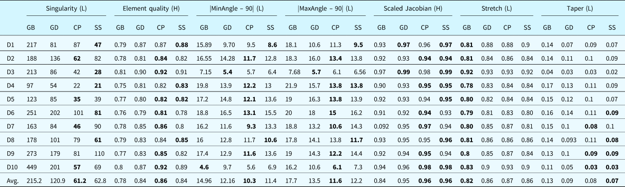
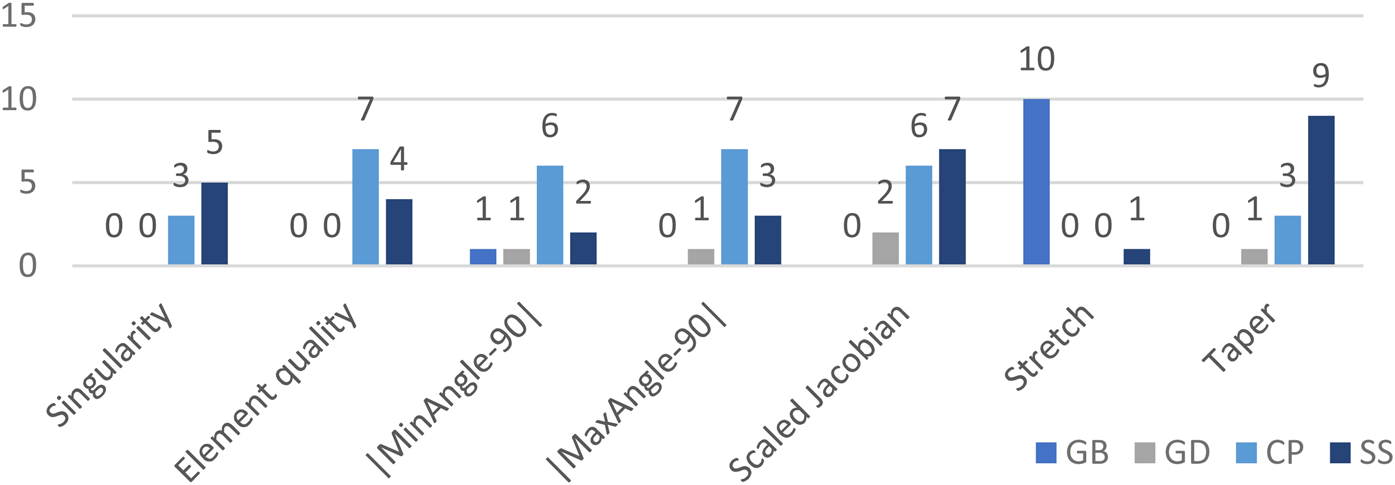
Comparing with three existing meshing approaches, the main contribution of this proposed system includes: (1) to construct element extraction rules by replacing the conventionally inefficient and incomplete search of heuristic knowledge with an automatic self-learning schema; (2) to achieve high performance in all the quality measurement indices with the highest score in the metrics of Taper and Scaled Jacobian; (3) to eliminate the need for in-depth knowledge in computational geometry, which makes it algorithm developer-friendly; and (4) to provide insights about smart designing of smart system.
The rest of this paper is organized as follows. Section “Smart designing of the smart element extraction system” discusses the smartness of the proposed element extraction system and the smart designing embedded in the system. The proposed system is presented in Section “A self-learning system for element extraction” using quad mesh generation. Section “Experiments” compares the proposed system's performances with the other three widely adopted methods. Section “Discussion” discusses the practical and theoretical benefits of this research. Finally, Section “Conclusions” concludes this paper.
Smart designing of the smart element extraction system
To address the challenge identified in Section “Introduction”, we adopt a concept of smart designing of smart systems. A smart system has two important properties: (1) making adaptive decisions corresponding to various environmental situations, and; (2) self-evolving to improve the system performance (Akhras, Reference Akhras2000). For a smart element extraction system, its extraction rules should be adaptive to various domain boundaries and can self-evolve to achieve the overall mesh quality. This section introduces the smart element extraction system's design process, which is linked with two machine learning methods: reinforcement learning and artificial neural network, for self-evolving the element extraction rules.
How is the element extraction method smart?
What is the element extraction method?
Mesh generation is considered a design problem and can be resolved recursively into the atomic design and a sub-design problem (Zeng and Cheng, Reference Zeng and Cheng1991; Zeng and Yao, Reference Zeng and Yao2009). The quad mesh design should satisfy the following conditions: (1) each element is a quadrilateral; (2) the inner corner of each element should be between 45° and 135°; (3) the aspect ratio (the ratio of opposite edges) and taper ratio (the ratio of neighboring edges) of each quadrilateral should be within a predefined range; (4) the transition from a dense mesh to a coarse mesh should be smooth (Zeng and Cheng, Reference Zeng and Cheng1991; Zeng and Yao, Reference Zeng and Yao2009). Zeng and Cheng (Reference Zeng and Cheng1993) proposed a knowledge-based method, FREEMESH, to recursively extract quadrilateral elements following a domain boundary until the remaining boundary becomes a quadrilateral element, based on the recursive logic of design (Zeng and Cheng, Reference Zeng and Cheng1991). In FREEMESH, the atomic design is to generate an element in a specified boundary region, while the corresponding sub-design problem is to generate a good quality mesh over the domain by cutting the generated element from the original domain (see Fig. 1).

Fig. 1. Quad mesh generation process (Yao et al., Reference Yao, Yan, Chen and Zeng2005).
In extracting elements one by one, three types of element extraction rules (i.e., adding one, two, and three edges) are defined to construct a good quality element (see Fig. 2). The challenge is for these rules to generate a good quality element around the current domain boundary while guaranteeing that these design rules are still applicable to the remaining domain for the subsequent construction of good elements.

Fig. 2. Three primitive generation rules (Zeng and Cheng, Reference Zeng and Cheng1993).
How is the element extraction method smart?
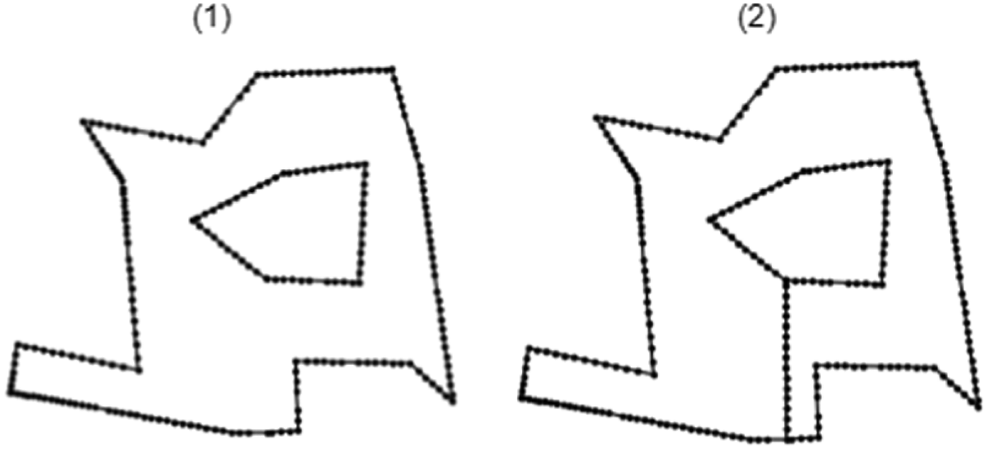
A smart system can make adaptive decisions corresponding to various environmental situations. For an element extraction method, the environment is domain boundaries, which keep changing throughout the entire mesh generation process. Even with a simple domain, the initial boundary can evolve into many complex intermediate boundary shapes. Following the process specified in Figures 1 and 3 shows an example element extraction process, where the initial boundary is shown in Figure 3 (1) and the final mesh is shown in Figure 3 (10). The intermediate boundaries could include various situations, which are not predictable.

Fig. 3. Changes of intermediate boundary shapes: all boundaries are represented in red lines from (2) to (9).
The smartness of element extraction systems lies in how various complex boundary shapes are processed by the three element-extraction rules shown in Figure 2. First, each edge in any boundary shape can be processed by one of those three extraction rules. The three rules define three kinds of patterns for a selected boundary edge V 1V 2 in a domain, as specified in solid lines in Figure 2a–c. The three rules are sufficient to process any environmental situation (boundary shapes). Secondly, among all the boundary edges, the system would be able to smartly pick up one edge and a corresponding rule to generate an element. In Figure 4, V 1, V 2, V 3 and V 4 are all the same for different environment situations while different rules are preferred if more conditions are considered from the environment. For instance, the boundary edge V 1V 2 is selected as the target edge in Figure 4a–f; the extraction rule in Figure 2c is applied in situations in Figure 4a,c,d; the extraction rule in Figure 2b is applied in situations in Figure 4b,e; and the last extraction rule in Figure 2a is applied in the situation in Figure 4f. This example demonstrates that it is challenging to select a proper rule even considering two more connected boundary points.

Fig. 4. Challenges in selecting a proper rule to extract an element for an edge V 1V 2.
Thirdly, when rules in Figure 2a or Figure 2b are selected for a boundary edge, the positioning of the newly added point(s) will be smartly determined according to its local surrounding environment situations so that a good element can be generated while the remaining boundary does not create an impossible situation for the three rules to process. For instance, Figure 5 shows the challenges in positioning the new point in extracting a new element for two base situations in Figure 4b,f. The red lines represent different remaining boundary shapes to form a complete domain boundary. Although Points B, B1, and B2 can form a better element in each situation, Points A, A1, and A2 are the optimal options due to the trade-off of quality of the element quality and the remaining boundary. The coordinates of newly added point(s) are adapted to various remaining boundary shapes.

In summary, the smart element extraction process is enabled by a knowledge-based reasoning process, where the three basic rules shown in Figure 2 can process complex 2D domain boundaries recursively. The method smartly extracts elements one by one adaptive to the situations implied in the current domain boundary.
How can the element extraction system be smartly evolving and designed?
As Figures 4 and 5 show, two major challenges exist to enable the smartness of an element extraction system, which are as follows:
(1) How to decide which of the three rules in Figure 2 should be applied for a selected edge (V 1V 2) from all kinds of geometric boundaries?
(2) For the first and second types of rules in Figure 2, how to determine relationships between the coordinates of the newly added points (V 3 and V 4; or V 3) and the geometric conditions surrounding the selected edge (V 1V 2)?
Conventionally, the questions above are answered manually by algorithm developers through a trial-and-error process. It is extremely difficult, costly, and time-consuming for human algorithm designers to develop such robust element extraction rules.
The element extraction rules can be smartly designed and evolving using machine learning algorithms, and many researchers attempted to combine machine learning algorithms with finite element methods. Those attempts include mesh density optimization with artificial neural networks (Chedid and Najjar, Reference Chedid and Najjar1996; Zhang et al., Reference Zhang, Wang, Jimack and Wang2020), node placement for existing quad elements by a self-organizing neural network (Manevitz et al., Reference Manevitz, Yousef and Givoli1997; Nechaeva, Reference Nechaeva2006), mesh design by an expert system (Dolšak, Reference Dolšak2002), remeshing structural elements by neural networks (Jadid and Fairbairn, Reference Jadid and Fairbairn1994), the relationship simulation between quad element state and forces (Capuano and Rimoli, Reference Capuano and Rimoli2019), triangular mesh simplification (Hanocka et al., Reference Hanocka, Hertz, Fish, Giryes, Fleishman and Cohen-Or2019), and mesh optimization to solve partial differential equation (Zhang et al., Reference Zhang, Cheng, Li and Liu2021). However, those methods do not directly focus on mesh generation and element extraction. There are a few works focusing on triangular mesh generation using neural networks (NNs). Pointer networks, (Vinyals et al., Reference Vinyals, Fortunato and Jaitly2015), are able to transform a sequence of points into a sequence of triangular mesh elements (three points). But it heavily relies the initial distribution of the points and cannot complete the meshing due to intersecting connections or low triangular element coverage. Papagiannopoulos et al. (Reference Papagiannopoulos, Clausen and Avellan2021) proposed a triangular mesh generation method with NNs using supervised learning. They trained three NNs based on the datasets of meshed domains by the Constrained Delaunay Triangulation algorithm (Chew, Reference Chew1989), to predict the number of candidate inner vertices (to form a triangular element), coordinates of those vertices, and their connection relations with existing segments on the boundary, respectively. The limitations of their method lie in that the overall mesh quality is doomed by the training data, and it cannot be applied to arbitrary and complex domain boundaries because of the fixing number of boundary vertices in the model input. They also cannot be applied to mesh generation or element extraction of quadrilaterals.
According to the nature of the problem, two machine learning algorithms can be exploited to enable the automatic evolution of element extraction rules. The first is Feedforward Neural Networks (FNNs), whereas the second is Reinforcement Learning (RL). The FNN can learn from given samples how to decide which rule should be applied and how to position the new point(s) for a new element when necessary. Yao et al. (Reference Yao, Yan, Chen and Zeng2005) improved the FREEMESH approach by introducing an artificial neural network (ANN) to learn the element extraction rules from a set of pre-selected samples of good quality quad meshes. The improved method eases the acquisition and application of these rules and could handle more complex domain boundaries. The trained model by ANN serves as the mapping function to transform the input (a specific boundary region) to output (rule type and a point), which is used to form an element following the FREEMESH construction process. This kind of system provides a smart designing mechanism that automatically generates smart rules to extract elements from any geometric domain.
With its abilities for trial-and-error learning, the RL models element extraction as a sequential decision-making problem. No samples are needed for the RL except that the mesh generation requirements need to be formulated into a reward feedback function. The RL will produce smart element extraction rules for generating high-quality quad meshes through self-learning and evolving. The system proposed in this paper combines these two different learning techniques: reinforcement learning and supervised learning (i.e., FNNs).
A self-learning system for element extraction
This section introduces a self-learning element extraction system, FreeMesh-S, which automatically generates mesh elements by self-learned extraction rules from a combination of an RL algorithm and an FNN. Quadrilateral element generation in single-connected 2D domains is used as an example to demonstrate this system. The subsequent subsection introduces how to formulate the element extraction into a reinforcement learning problem. Section “A2C RL network for element extraction based mesh generation” presents an RL algorithm, A2C, to learn to extract mesh elements by trial-and-error. Section “FNN as policy approximator for fast learning and meshing” elaborates how to utilize the FNN to accelerate learning extraction rules by supervised learning. Finally, Section “Summary” summarizes a general self-learning framework for element extraction.
Element extraction as a reinforcement learning problem
Architecture similarity between element extraction and reinforcement learning
The element extraction process in Figure 1 can be generalized into architecture, as shown in Figure 6. The mesh generator applies the extraction rules to a domain boundary and generates an element; the domain boundary will be updated by removing the extracted element, which is scored for its quality. This recursive process continues until mesh elements fill the domain. However, one must specify the mesh generator's extraction rules in advance. By formulating this process into an RL problem, the machine itself can automatically learn these extraction rules (i.e., the mesh generator).

Fig. 6. Element extraction architecture.
Reinforcement learning (RL) is a technique that enables an agent to learn from the interactions with its environment by trial-and-error via reward feedback from its actions and experiences (Kaelbling et al., Reference Kaelbling, Littman and Moore1996; Sutton and Barto, Reference Sutton and Barto2018). The hypothesis behind RL is that all the goals can be represented by the maximization of the expected cumulative reward. As is shown in Figure 7, the agent, at each time step t, observes a state S t from the environment, and conducts an action A t applied to the environment. The environment responds to the action and transits into a new state S t+1. It then reveals the new state and provides reward Rt to the agent. This process forms an iteration and repeats until a given condition is satisfied (i.e., the RL problem is solved).

Fig. 7. Architecture of reinforcement learning (Sutton and Barto, Reference Sutton and Barto2018).
It can be seen from Figures 6 and 7 that element extraction and reinforcement learning bear a similar framework of problem-solving. As illustrated in Figure 8, the mesh generation process shown in Figure 6 has the same architecture as the RL process does, and the mesh generation process can be seen as an instance of an RL process. In the context of element extraction, the agent is a mesh generator; the environment is a domain boundary to mesh; the state of the environment consists of a set of focused vertices and edges in the boundary; an action to take by the agent is to extract an element from an edge in the state; the reward is the combination of qualities of both the current extracted element and the remaining boundary; a policy of the agent guides the selection of a specific action; the agent's goal is to maximize the aggregated rewards – the total quality of all extracted elements and their corresponding boundaries.

Fig. 8. Element extraction process as reinforcement learning.
Formulation of the element extraction problem in the reinforcement learning framework
In RL, how the learning agent behaves (to select an action at each state) is described as the agent's policy. Mathematically, a policy is represented as a probability distribution over all possible actions at each state, denoted as π(a|s). A state's value is the expected future rewards starting at that state, which determines how beneficial for the agent to enter that state. A value function is designed to estimate the value for each state. The value function  $V^\pi ( s )$ of a state S t under a policy π is formally denoted as,
  $V^\pi ( s ) = E[ {G_t{\rm \vert }S_t = s, \;\;\pi }] , \;$ for any s ∈ S , where S is a set of environment states; and G t is a discounted sum of the sequence of rewards achieved over time, which is calculated by,
 $$G_t = \mathop \sum \limits_{k = t + 1}^T \gamma ^{k-t-1}R_k, \;$$
where 0 ≤ γ ≤ 1 is a discount rate, and T is a final time step. The value function of an action at a state under a policy can be expressed as  $Q^\pi ( {s, \;\;a} ) = E[ {G_t{\rm \vert }S_t = s, \;A_t = a, \;\;\pi }].$ These value functions can be estimated from experience with different methods. Policy and value functions are essential for almost every RL algorithms.
Mathematically, the RL is a sequential decision-making process, which can be formalized as a Markov Decision Process (MDP) consisting of a set of environment states S, a set of possible actions A(s) for a given state s, a set of rewards R, and a transition probability P(S t+1 = s', R t+1 = r|S t = s, A t = a) where s', s ∈ S, a ∈ A(s), r ∈ R, s' is the new state at t + 1 and r is the reward after action a at state s. The transition probability indicates that the current state is only dependent on the preceding state and action, the so-called Markov property, thereby defining the MDP dynamics. This requires that the state contain information about the past interactions that could distinguish the future and the present. The MDP and agent then produce a sequence [S 0, A 0, R 0, S 1, A 1, R 1, S 2, A 2, R 2, … ]. In general, the MDP framework can be applied to various problems in many ways because of its flexibility. Once a goal is represented as agents’ choices, the basis for choice from the environment, and a reward measurement of the goal, it can be formalized as an RL problem. Existing reinforcement learning algorithms can be categorized into three types: policy-based, value-based, and model-based methods (Kaelbling et al., Reference Kaelbling, Littman and Moore1996; Sutton and Barto, Reference Sutton and Barto2018), which learn policies, value functions, and models (Grondman et al., Reference Grondman, Busoniu, Lopes and Babuska2012). Deep reinforcement learning (DRL) intends to make behavioral decisions through learning from the experience of interacting with the environment and from the evaluative feedback (Littman, Reference Littman2015).
Mathematically, as RL does, the element extraction process can also be represented as an MDP, which consists of a set of boundary environment states S, a set of possible actions A(s) in state s to form an element for each boundary state, a set of rewards R, and a state transition probability P(s', r|s, a). The extraction process will produce a sequence [S 0, A 0, R 0, S 1, A 1, R 1, S 2, A 2, R 2, … ], where the notations are explained as follows:
-
t: denotes the index associated with the time step of element extraction;
-
S t: the partial boundary of the domain (at time t) from which the tth element will be extracted;
-
A t: the action to produce the tth extracted element, which consists of four vertices of the extracted element.
This process shows the natural alignment of the element extraction method with reinforcement learning.
Correspondingly, the three rules, which are used to extract elements in Figure 2, can be viewed as three actions: (a) to add two new vertices and three edges; (b) to add one new vertex and two edges; (c) to add just one edge. The determination of which rule to apply and especially where to position a candidate vertex to form a high-quality element is highly challenging because the position of a new vertex has substantial impacts on the quality of meshing in the future steps. These actions address the two questions raised in Section “How can the element extraction system be smartly evolving and designed?”.
In this work, we focus on using RL to select the optimal position of a candidate vertex, and the action is defined as locating a vertex position. In this way, the action space could be a two-dimensional continuous domain. The policy that needs to be learned with RL is the element extraction rule, which maps a state to an action (positioning the new vertex). The full state of the environment at time t would consist of all boundary vertices at the time. However, not all vertices are equally useful for extracting a new element. Zeng and Cheng (Reference Zeng and Cheng1993) identified a small set of vertices on the current boundary, which are highly relevant to constructing a new element. We select this partial boundary to represent the state, making computing much more efficient. This selected partial boundary denoted as S t, is composed of four parts (1) a reference point, P 0, which is a vertex selected from the current boundary and will be used as the relative origin for the new element to be constructed and extracted; (2) n neighboring vertices in the right side, where n = 2 in this paper; (3) n neighbor vertices in the left side, where n = 2; (4) three neighboring points  $P_{\theta _1}$,
  $P_{\theta _2}$, and
  $P_{\theta _3}$ in the fan-shaped area θ 1, θ 2, and θ 3 with radius d, as shown in Figure 9. This partial boundary is denoted as:
 $$S_t = \{ P_{l2}, \;\;P_{l1}, \;\;P_0, \;{\rm \;}P_{r1}, \;\;P_{r2}, \;\;P_{\theta _1}, \;P_{\theta _2}, \;P_{\theta _3}\} , \;$$
which is still a high dimensional continuous domain, but its dimension is significantly reduced from the full boundary. We treat this partial boundary as the state partially observed by the agent (Kaelbling et al., Reference Kaelbling, Littman and Moore1996).
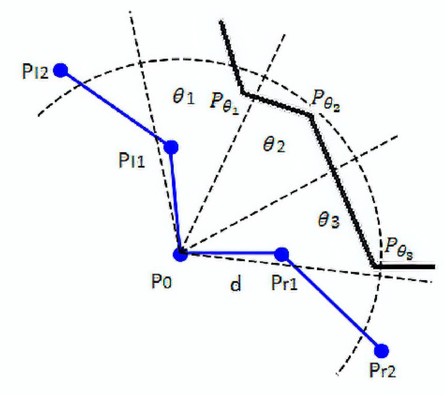
Fig. 9. Partial boundary.
Regarding reward, we define it as the combination of qualities of both the extracted element and the remaining boundary because their trade-off is essential to the overall quality of the final mesh. The reward details will be defined in Section “Reward function”.
Regarding the agent's policy and the value function of a state (or action under a state), as discussed earlier, the position of a new vertex for a new element has substantial impacts on the quality of meshing in the future steps; it is highly challenging to find an optimized policy to locate the vertex position and to find a reasonable estimation of that position. Both an optimal policy and the value function are unknown to the agent but can be approximated with a parameterized function by learning from experience. For this reason, the advantage actor-critic method is used in this paper.
A2C RL network for element extraction- based mesh generation
The overall architecture of the advantage actor-critic (A2C) is shown in Figure 10. The “actor” mimics the policy in the architecture, and the “critic” mimics state value functions. We use an A2C network-based agent to interact with the environment and gradually generate high-quality elements by trial-and-error learning. The following subsections will introduce the basics of the A2C method and explain how to generate mesh elements with the A2C method.

Fig. 10. A2C agent architecture for element extraction.
A2C
The RL problem is to learn how to select an action at each state over time to maximize the accumulated reward G t, which is a discounted sum of the sequence of rewards achieved over time, as shown in Eq. (1). Actor-critic is a subclass of policy-gradient methods, which learns approximations to both policy and value functions (Grondman et al., Reference Grondman, Busoniu, Lopes and Babuska2012; Sutton and Barto, Reference Sutton and Barto2018). Policy-gradient methods directly optimize an agent's actions without consulting a value function. Policy-gradient methods are via learning a parameterized policy  $\pi _\theta$, where θ is the policy's parameter vector. The probability that an action a has been taken in state s at time t with policy parameter θ is represented as π(a|s, θ) = Pr{A t = a|S t = s, θ t = θ}. The general idea is to increase the probability of actions being taken in each state when they have high optimality. The performance of the policy can be denoted as
  ${\cal J}( \theta ) = V^{\pi _\theta }( s )$, which is calculated by
 $$V^{\pi _\theta }( s ) = \mathop \sum \limits_{a\in A} \pi _\theta ( a\vert s) \mathop \sum \limits_{{s}^{\prime}\in {\boldsymbol S}} \Pr ( {{s}^{\prime}\vert s, \;\;a} ) \{ {r + {\rm \;}\gamma V^{\pi_\theta }( {{s}^{\prime}} ) }\} , \;$$
when every episode starts in state s. r is the reward after action a at state s. According to the policy gradient theorem, the gradient of this performance is denoted as,
 $$\nabla _\theta {\cal J}( \theta ) \propto \mathop \sum \limits_s d( s ) \mathop \sum \limits_a Q^\pi ( {s, \;\;a} ) \nabla _\theta \pi ( {a{\rm \vert }s, \;\theta } ) , \;$$
where d(s) is a state distribution under policy  $\pi , \;\;Q^\pi ( {s, \;\;a} )$ is state-action value function under policy π. The gradient-ascent algorithm improves the policy as
 $$\theta _{t + 1} = \theta _t + \alpha \nabla _\theta {\cal J}( \theta ) , \;$$
where α is a step size.
We can estimate the performance gradient using Monte Carlo sampling, which is proportional to the actual gradient. The gradient can then be represented as,
 $$\nabla _\theta {\cal J}( \theta ) \;\propto E\left[{\mathop \sum \limits_a Q^\pi ( {S_t, \;\;a} ) \nabla_\theta \pi ( {a{\rm \vert }S_t, \;\theta } ) } \right] = E[ {G_t\nabla_\theta {\rm ln}\pi ( {A_t{\rm \vert }S_t, \;\theta } ) }] , \;$$
where S t and A t are sampled state and action at time t, G t is the return after t, and; E[.] is the expected value of the expression with random variables S t and A t in the Monte Carlo sampling. The gradient-ascent algorithm could be,
 $$\theta _{t + 1} = \theta _t + \alpha G_t\nabla _\theta {\rm ln}\pi ( {A_t{\rm \vert }S_t, \;\theta } ).\;$$
 Because the variance of return is high in Monte Carlo policy gradient, the learned value function can reduce the gradient variance and provide an informative direction for policy optimization. The actor represents the learned policy, whereas the critic is the learned value function. The critic estimates the state-action value function as an approximator with parameters w, that is  $\hat{Q}^{\pi _\theta }( {s, \;\;a; \;w} ) \;\approx Q^{\pi _\theta }( {s, \;\;a} )$, where
  $Q^{\pi _\theta }( {s, \;a} )$ is the state-action value function using policy
  $\pi _\theta$. Correspondingly,
  $V^{\pi _\theta }( s )$ can be estimated as
  $\hat{V}^{\pi _\theta }( {s; \;w} ) = E_{a\sim \pi }[ {{\hat{Q}}^{\pi_\theta }( {s, \;\;a; \;w} ) }]$. By introducing an advantage function to the critic,
 $${\rm \;}A^{\pi _\theta }( {s, \;{\rm \;}a} ) = Q^{\pi _\theta }( {s, \;a} ) -V^{\pi _\theta }( s ) , \;$$
In this way, the policy optimization will be more directional. It leads to the advantage actor-critic (A2C) method. The gradient is changed to the following:
 $$\nabla _\theta {\cal J}( \theta ) \propto E\left[{\mathop \sum \limits_a {\rm }A^{\pi_\theta }( {s, {\rm \;}a} ) \nabla_\theta {\rm ln}\pi ( {a{\rm \vert }S_t, \;\theta } ) } \right].$$
The actor updates the policy parameters by
 $$\theta _{t + 1} = {\rm \;}\theta _t + \alpha A^{\pi _\theta }( {S_t, \;\;A_t} ) \nabla _\theta {\rm ln\;}\pi ( {A_t{\rm \vert }S_t, \;\theta } ).$$
The critic updates its weights by
 $$w_{t + 1} = {\rm \;}w_t + \beta A^{\pi _\theta }( {S_t, \;\;A_t} ) \nabla _w\hat{V}^{\pi _\theta }( {s; \;w} ).$$
 By the definition of the value function  $V^{\pi _\theta }( s ) , \;$ advantage function
  $A^{\pi _\theta }( {S_t, \;\;A_t} )$ can be estimated as
 $$\delta _t = R_{t + 1} + \gamma \hat{V}^{\pi _\theta }( {S_{t + 1}; \;w} ) -\hat{V}^{\pi _\theta }( {S_t; \;w} ) , \;$$
which is also called temporal difference (TD) error for state value at time t. For a more detailed description of the A2C model please refer to (Sutton and Barto, Reference Sutton and Barto2018). For the specific description of our A2C RL model for mesh, please refer to the next subsection. Advantage Actor-Critic (A2C) network is a class of A2C model, in which an artificial neural network is used as an approximator for the policy or the value function. We use this approach for mesh generation.
A2C RL network for element extraction
In the proposed self-learning element extraction system, the A2C network is responsible for the preliminary sampling of the element extraction rules (a set of three rules in Figure 2). Its network structure is shown in Figure 11. The actor and critic are the two heads of the network and share the same input and hidden layer. The input is the partial boundary S t. The value head of the critic is the estimation of the state-value function. The policy head of the actor will output two variables (i.e., two means) to form two normal distributions in which both the variances are set to 1, to sample the coordinates, x and y, of the candidate point, respectively. The training process of the A2C network is illustrated in Algorithm 1. For a given 2D domain environment, the A2C network updates the parameters of the actor and the critic during each episode using the temporal difference (TD) method [i.e., Eq. (12)]. Each episode terminates when the domain is full of quadrilateral elements or exceeds the maximum step. The episode number M indicates the maximum iteration. The maximum step in each episode is defined by T. Symbol λ is the discount factor during reward accumulation.
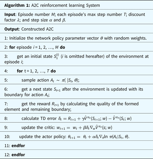

Fig. 11. A2C network structure. In general, the actor will simulate three primitive rules, as shown in Figure 2a–c. In the current implementation, the extraction rule in Figure 2a is not considered, and it will be implemented in the next version of the system.
State representation
The state is the actor's observation of the environment, which is defined as a partial boundary S t, expressed as Eq. (2). Two fundamental steps are needed to determine which part of the boundary is considered the state: (1) to identify the reference point P 0 from the existing boundary; and (2) to find the remaining points according to Eq. (2). A new element will be extracted around this formed partial boundary. First, the reference point is calculated by iterating all the points on the boundary, computing the angle of each point formed by its left and right connected points, and selecting the point having the least angle as the P 0. Then, the other points in S t will be determined by Eq. (2). The absolute coordinates of all points selected for representing a state will be transformed into a new coordinate system that assumes the reference point P 0 as the origin, and the vector from the reference point to the first neighboring point along the counter-clock direction as the unit vector, along the positive direction of the x-axis (Yao et al., Reference Yao, Yan, Chen and Zeng2005). The transformation (i.e., rotation, scaling, and transit) from the original coordinate system Oxy to the new one O'x'y' is shown in Figure 12, and can be represented as:
 $$\eqalign{\left({\matrix{ {{x}^{\prime}} \cr {\matrix{ {{y}^{\prime}} \cr 1 \cr } } \cr } } \right) &= \left[{\matrix{ {{\rm cos}\;\theta } & {{\rm sin}\;\theta } & 0 \cr {-{\rm sin}\;\theta } & {{\rm cos}\;\theta } & 0 \cr 0 & 0 & 1 \cr } } \right]\;\;\left[{\matrix{ {\displaystyle{1 \over d}} & 0 & 0 \cr 0 & {\displaystyle{1 \over d}} & 0 \cr 0 & 0 & 1 \cr } } \right]\;\;\left[{\matrix{ 1 & 0 & {-x_0} \cr 0 & 1 & {-y_0} \cr 0 & 0 & 1 \cr } } \right] \cr &\quad \times \left({\matrix{ x \cr {\matrix{ y \cr 1 \cr } } \cr } } \right),} \;$$
 $$d = \sqrt {{( {x_0-x_{r1}} ) }^2 + {( {y_0-y_{r1}} ) }^2}.$$
Fig. 12. Coordinate transformation.
Reward function
The actor will receive reward feedback from the environment to indicate how good the performed action is at the current state S t, which the environment in RL refers to as the mesh domain boundary. The reward function is defined as follows:
1) if the point (action) is outside the domain, the reward is set to be −0.1;
2) if the generated element has straddled segments with itself or other elements, as shown in Figure 13, the reward is set to be −0.1;
3) if the element has no situation with (1) and (2), the reward is the combination of current ith element quality
 $\eta _i^e$ and the quality of the remaining boundary $\eta _i^b$, which is calculated by $\sqrt {\eta _i^e \ast \eta _i^b }$. The element quality $\eta _i^e$ is measured by both its edge quality and angle quality, and calculated as follows, which are adapted from (Zeng and Yao, 2009),(14)$$\eta _i^e = \sqrt {q^e\ast q^a} , \;$$(15)$$q^e = \root 4 \of {\mathop \prod \limits_{\,j = 1}^4 {\left({\displaystyle{{l_j} \over {\sqrt {A_i} }}} \right)}^{{\rm sign}\left({\sqrt {A_i} -l_j} \right)}} , \;$$(16)$$q^a = \root 4 \of {\mathop \prod \limits_{\,j = 1}^4 \left({1-\displaystyle{{\vert {a_j-90} \vert } \over {90}}} \right)} , \;$$


where q e refers to the quality of edges of this element; l j is the length of the jth edge of the element; A i is the area of the ith element; q a refers to the quality of the angles of the element; and a j is the degree of jth inner angle of the element. The quality  $\eta _i^e$ will range from 0 to 1, which is better if greater. Examples of various element qualities are shown in Figure 14.

Fig. 13. Invalid situations of the element. P 0 is the reference point, and P is the newly generated point.

Fig. 14. Different quality of elements.
The quality of remaining boundary,  $\eta _i^b$, is calculated as follows,
 $$\eta _i^b = \sqrt {\mathop \prod \limits_{k = 1}^2 \left({\displaystyle{{{\rm Min}( {\theta_k, \;60} ) } \over {60}}} \right)} , \;$$
where θ k refers to the degree of the kth generated angle, as shown in Figure 15. The quality  $\eta _i^b$ also ranges from 0 to 1, which the higher value is, the better.

Fig. 15. New boundary angles.
Finally, we have the reward function as
 $$R_t = \left\{{\matrix{ {-0.1, \;\;{\rm if\;the\;generated\;point\;is\;outside\;the\;domain\;or}} \hfill \cr {\;{\rm the\;formed\;elements\;has\;straddled\;segments}; \;} \hfill \cr {\sqrt {\eta_i^e \ast \eta_i^b } , \;\;{\rm otherwise}.\;\;\;\;\;\;\;\;\;\;\;\;\;\;\;\;\;\;\;\;\;\;\;\;\;\;\;\;\;\;\;\;\;\;\;\;\;\;\;\;\;\;\;\;\;\;\;\;\;\;\;\;\;\;\;\;\;\;\;\;\;\;\;\;\;\;\;\;} \hfill \cr } } \right.$$
To have a negative reward prevents the actor from performing inappropriate actions and generating invalid elements. Once the actor generates a valid element, it will immediately receive a reward value to tell how good that action is. This is a stepwise reward signal, which smoothly guides the actor to achieve the final goal. The reason to consider both the quality of the current element and the remaining boundary is that the actor needs to learn the trade-off between them to achieve an overall good mesh quality and complete the meshing task.
Actor representation
In a fully observable MDP, the agent observes the true state of the environment at each time t and acts according to a parameterized policy  $\pi _\theta$. The actor constantly chooses actions and produces the best one for a given environmental state S t overtime. Typically for type (b) action shown in Figure 2, the selected action A t (line 5 of Algorithm 1) is to sample a point P t within a specified area with the reference point P 0 as the center. The selection is sampled from the parameterized policy,
  $A_t = P_t\sim \;\pi _\theta ( {s_t} )$. Finally, a new element is formed by four points, P t, P l1, P 0, and P r1, after the environment receives the point P i.
The actor will also update (line 10 of Algorithm 1) the policy distribution at each time step concerning the parameter vector θ by using the sampled policy gradient:
 $$\nabla _\theta {\cal J}( {\pi_\theta } ) = {\rm \;}\mathop \sum \limits_{s, {\rm \;}a} [ {\nabla_\theta {\rm ln}\pi_\theta ( {a{\rm \vert }s} ) A^{\pi_\theta }( {s, {\rm \;}a} ) }] , \;$$
in which the direction  $A^{\pi _\theta }( {s, \;{\rm \;}a} )$ is suggested by the critic (Section “Critic representation”).
Critic representation
The critic is used to observe the states and rewards from the environment and estimates the value function  $\hat{V}^{\pi _\theta }( {s; \;w} )$ accounting for both immediate and future reward to be received by the following policy
  $\pi _\theta$. The value function will determine whether the selected point's position can achieve the best performance in both the quality of the extracted element and the remaining boundary in the long run. The advantage function is adopted to reduce state value estimation variance and produce a positive direction for optimization, as shown in Eq. (8). Since the temporal-difference (TD) error, defined in Eq. (12), can be used as the unbiased estimation of the advantage function, it will guide the updating of parameter vector θ in the actor. The updating of the critic's parameters in Figure 10 is shown in Line 9 of Algorithm 1.
FNN as policy approximator for fast learning and meshing
A2C network can acquire new knowledge with a slow trial-and-error process; hence, it is practically infeasible to do element extraction directly using RL. To address this challenge, A2C is used to generate good meshes to extract successful (state, action) pairs as samples for training a multilayer FNN. The FNN can be seen as an RL policy approximator. The architecture of the integrated approach is shown in Figure 16.

Fig. 16. FNN agent architecture.
The architecture in Figure 16 provides a policy-only approach without consulting value functions. This entire process simulates the human learning process, which acquires successful samples from trial-and-error, extracts experience from those samples, and enhances the extracted experience's decision-making ability. It is a novel combination of two methods to form a human-like learning schema to solve the mesh generation problem. The learning process consists of experience extraction and FNN learning. Experience extraction is a prerequisite for the FNN component. When the learning finishes, the trained model applies to various domain boundaries for generating mesh elements.
FNN learning
The FNN module can learn from the acquired data from the experience extraction module to (1) decide which extraction rule should be applied and (2) determine the position of the newly generated point for a new element when necessary. Its network structure is shown in Figure 17 and mathematically described as follows (Yao et al., Reference Yao, Yan, Chen and Zeng2005):
 $$[ {{\rm typ}{\rm e}_i, \;\;P_i}] = f( [ P_{( {l, \;N} ) }, \;\;\ldots , \;P_{l2}, \;\;P_{l1}, \;\;P_0, \;\;P_{r1}, \;\ldots , \;\;P_{( {r, \;N} ) }, \;P_{\theta _1}, \;P_{\theta _2}, \;P_{\theta _3}]), \;$$
where typei is the output type, as shown in Figure 18, which equals to one of the three values (i.e., 0, 1, and 2); P i is the output point, consisting of (x i, y i); the input points are the state; and N equals 2 in this paper. The objective function used in FNN is denoted in the following formula:
 $${\rm MSE} = \displaystyle{1 \over n}\;\mathop \sum \limits_i^n [ {{( {x_i-\widetilde{{x_i}}} ) }^2 + {( {y_i-\widetilde{{y_i}}} ) }^2 + {( {{\rm typ}{\rm e}_i-\widetilde{{{\rm typ}{\rm e}_{\rm i}}}} ) }^2}] , \;$$
where  $\widetilde{{x_i}}, \;\;\widetilde{{y_i}}, \;\;\widetilde{{{\rm typ}{\rm e}_{\rm i}}}$ are the FNN model output for ith input and MSE is the sum of the mean squared errors of these three variables.

Fig. 17. FNN module structure.

Fig. 18. Three types of outputs.
Through supervised learning, these element extraction rules are quickly acquired. The trained model can easily distinguish which rule should be applied under a specific environment state (input) and can generate a point (output) to form a high-quality element correspondingly. In this way, the experience is transferred from the slow trial-and-error A2C process to the fast one-step FNN. This process also simulates the human decision process as specified by Kahneman (Reference Kahneman2011).
Experience extraction
The experience extraction (EE) module intends to extract samples from existing elements derived from the A2C model for the FNN model training. A sample here is an instance of extraction rules, which is represented by the mappings from a state (input) to the output type and point, as shown in Figure 17. For the meshing result generated in each episode by the A2C, EE will check if they are qualified to be extracted as samples. Two criteria are hence used to determine the quality of samples: (1) element quality  $\eta _i^e$ is used to filter out unqualified elements, and; (2) the number of total qualified elements in a meshing result of A2C should exceed a threshold η.
An example of the sample extraction process is shown in Figure 19. A trajectory stops when no valid elements are generated within the maximum step T. A trajectory from the A2C module is illustrated in Figure 19a, which meets the second criterion (e.g., η = 20) as previously mentioned. Each element has a property defined by a tuple <element id; element quality>, where Element id is defined as the order of the element extracted. Many mesh elements can be used for EE based on the first criterion (i.e.,  $\eta _i^e > 0.7$), such as elements 0, 1, 3, 7, 14, 15, 19 and 23 while some other elements will be excluded, such as 5, 12, 13, and 17. For example, element 15 with element quality 0.91 in Figure 19a is used to show the experience extraction process. Three types of extracted samples are shown in Figure 19b–d. Eight points are selected as the input for each rule type, where points P l2, P l1, P 0, P r1, and P r2 (in red), are points in the boundary from left to right with P 0 as the reference point, and points
  $P_{\theta _1}$,
  $P_{\theta _2}$, and
  $P_{\theta _3}$ (in blue) are collected from the fan-shaped area θ 1, θ 2 and θ 3 with radius d=3 with the unit length being P 0P r1, as shown in Figure 9; and the output point is chosen as P i (in black). It should be noted that the point P r2 is P i in Figure 19c and the point P l2 is P i in Figure 19d.
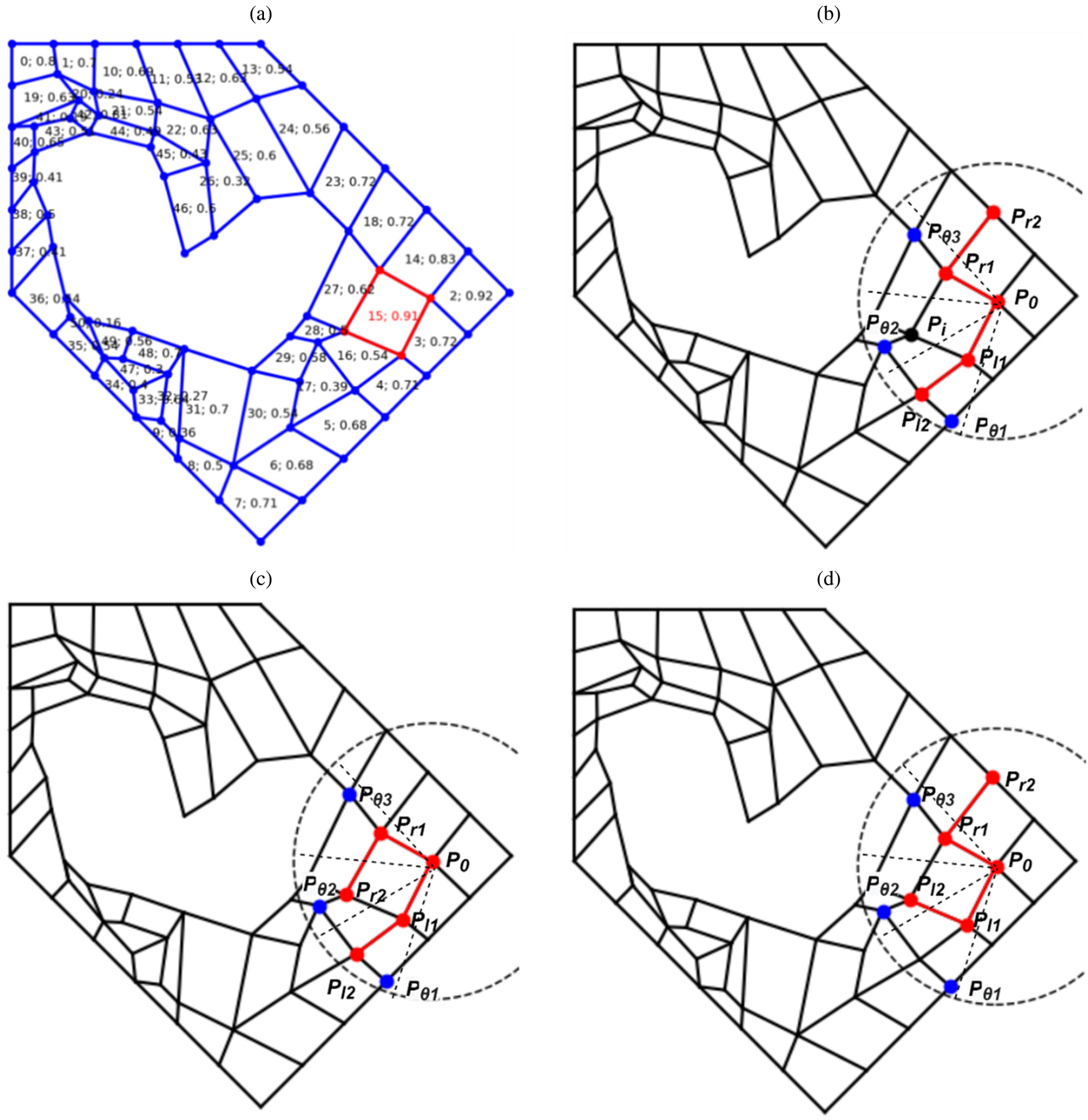
Fig. 19. Example of experience extraction of one element. In (a), each element has a tuple < element id; element quality > inside, where element id refers to the generation order of the element; and element quality is calculated by  $\eta _i^e$; (b)–(d) show three types of patterns collected for training samples: (b) type 0; (c) type 1; (d) type 2.
The input-output pair for each training sample will be arranged according to Eq. (20). Ten training samples with the same reference point and output point are shown in Table 1. Those input-output pairs will be normalized and transformed from the original coordinate system Oxy to the new one O'x'y' (see Fig. 12). The transformation results are shown in Table 2. Consequently, all the sampling points’ coordinates are constructed into the same scale, and their relationships remain unchanged.
Table 1. Examples of extracted samples for element 15: the reference point P 0(x 0, y 0) and output point P i(x i, y i) are the same across these samples, respectively

Table 2. Examples of extracted samples in Table 1 after coordinate transformation following Eq. (13)

The extraction process will be repeated for all the qualified elements in an existing mesh to gather training samples. In this way, a large number of training data can be easily extracted with a single mesh. Furthermore, the training data contains sufficiently diversified situations in meshing any complex geometric domain.
Summary
Using quadrilateral mesh generation as an example, the self-learning element extraction system, FreeMesh-S, demonstrates how the extraction rules are acquired by combining an A2C and an FNN. The general architecture is illustrated in Figure 20. Through considering the mesh generation as a design problem, three atomic design rules (i.e., three extraction rules) are proposed to recursively extract quadrilateral elements by Zeng and Cheng (Reference Zeng and Cheng1993), which are complete and sufficient to mesh various complex boundary shapes. Given these defined rules, the agent of RL (i.e., A2C here) learns their transition relationships through continuously self-evolving, known as the policy. The FNN serves as a policy-only approach to extract samples from those high-quality elements from the trial-and-error, enabling the agent to choose one of the three extraction rules to apply and position the coordinates of newly added points.

Fig. 20. Proposed self-learning system FreeMesh-S: architecture.
The generalized architecture is not only limited to quad mesh generation, but any problem that can be formulated into atomic design problems and sequential decision-making problems.
Experiments
To comprehensively evaluate the learned element extraction rules’ performance by the proposed self-learning system, FreeMesh-S, two experiments were conducted. Experiment 1 tests the training's performance and the impact of the training parameters on the quality of the generated mesh. Experiment 2 compares the quality of meshes by FreeMesh-S against three widely adopted meshing approaches over ten predefined 2D domain boundaries. The following subsections will discuss the experiment details and results.
Experiment settings
Experimental domain boundaries
To provide comprehensive and various challenging situations for meshing, testing domain boundaries are chosen based on whether a boundary includes sharp angles, bottleneck regions, unevenly distributed segments, and holes. Hence, ten domain boundaries are selected to test the proposed system's performance (see Fig. 21 and Table 3).

Fig. 21. 10 experimental domains.
Table 3. Description of 10 testing domains

Mesh performance evaluation metrics
The meshing performance is measured by seven mesh quality metrics, including six geometric metrics and one topological metric, as shown in Table 4.
Table 4. Mesh quality metrics

Seven quality metrics are:
• Singularity: the number of irregular nodes in the interior of a mesh. A node is considered irregular if it does not have four incident edges (Verma and Suresh, Reference Verma and Suresh2017);
• Element quality η e: an index defined by Eq. (14);
• |MinAngle-90|: the absolute differences between the smallest internal angle of an element and 90°; The smaller differences imply a better element;
• |MaxAngle-90|: the absolute differences between the largest internal angle of an element and 90°; The smaller differences imply a better element;
• Scaled Jacobian: the minimum Jacobian (Knupp, Reference Knupp2000) at each corner of an element divided by the lengths of the two edge vectors, which varies from minus one to plus one, where a higher value implies a better element; the negative value, typically, means the element is inverted;
• Stretch: an index referring to the ratio between the shortest element edge length and the longest diagonal length;
• Taper: the maximum absolute difference between the value one and the ratio of two triangles’ areas are separated by a diagonal within a quadrilateral element. The smaller value represents that the element becomes closer to a triangular shape.
All the metrics are averaged for all elements in the mesh, respectively. Some indices (e.g., scaled Jacobian, stretch, and taper) are calculated using Verdict software (Pébay et al., Reference Pébay, Thompson, Shepherd and Grosland2008).
Experiment 1: training effectiveness and efficiency
The proposed self-learning meshing system's training consists of two parts: A2C model training and FNN model training. For the A2C network, the actor and critic share the same hidden layer (128 nodes). Since the environment state consists of 8 2D points, the input layer has 16 nodes. For the action is the coordinates of the candidate point, which is continuous in a 2D space, the policy is represented by two normal distributions to estimate x, y coordinates, respectively. Two mean values of the normal distributions are the actor's outputs, and two variance values are set to 1. The final x, y coordinates are sampled from these two distributions according to the obtained mean and variance pairs. To accelerate the learning speed, the sampled x, y coordinates are clipped into [-1.5, 1.5]. The learning rate of 0.0001 is set for the network, and the reward discount rate is set as 0.99.
Self-sampling and evolving of A2C and FNN training
There are two steps to complete the FNN network's training, as is shown in Figure 22. In Step 1, the A2C module will generate a mesh, covering only a partial domain to mesh. The generated mesh is then used to produce initial training samples for FNN. In Step 2, the FNN will be trained, applied, and further evolved.

Fig. 22. Model training process.
In this presented research, an empty domain, such as shown in Figure 23a, is used to generate elements without any prior knowledge about the parameters in the extraction rules in Figure 2. The A2C network can generate high-quality elements in the domain after some rounds of trial and error. Those high-quality elements in each episode of training can be extracted as training samples for the FNN network, which can be reused for the boundary of different shapes. Figure 23d–f are episodes that include sufficient good samples to train the FNN. An episode can be selected as a source for element sampling if two criteria are met:  $\eta _i^e$ > 0.7 and η > 20, as introduced in Section “Experience extraction”.
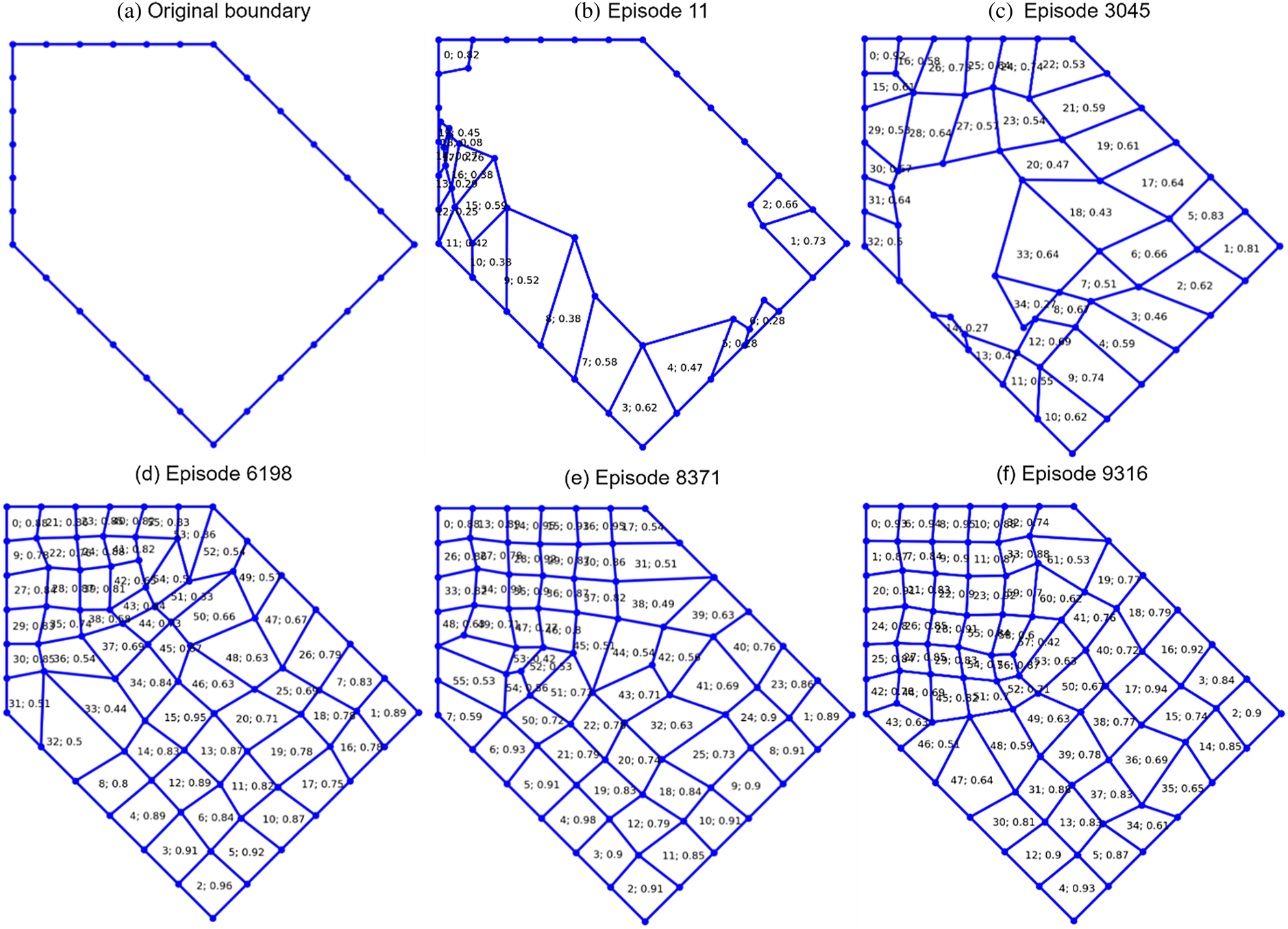
Fig. 23. Partial results of sampling.
Table 5 shows the total number of elements (#tE), number of valid elements (#vE), number of extracted samples (#eS), and the number of samples per valid element (#S2E) for each episode. The samples are extracted using the experience extraction (EE) module introduced in Section “FNN learning”. It can be seen from Table 5 that the episode in Figure 23d has 37 valid elements, which allows the extraction of 10,369 different samples (see the extraction process in Figure 19 ), where the number of samples per valid element has reached 280. Similar information can be observed in Figure 23e, f. This significant number of leverage over an element brings the EE module's tremendous efficiency and effectiveness in collecting samples. This effectiveness and efficiency in data collection ensure that the FNN model can be sufficiently trained.
Table 5. Extracted sample records from valid elements

#tE – total number of elements;
#vE – number of valid elements with quality η e > 0.7;
#eS – number of extracted samples;
#S2E – the number of samples per valid element
Then trained FNN model can be applied to another domain, such as domain D2, to do the meshing even though the extracted samples are from a different domain (see Fig. 23a). The meshing result of this FNN model is shown in Figure 24.

Fig. 24. The first meshing result of the FNN model.
The meshing, however, is not complete in this domain. In step 2 of the training process, as illustrated in Figure 22; therefore, there is a self-evolving process of the FNN model by learning from the meshing results generated by itself. While repeating step 2, the element extraction rules simulated by the model are gradually evolved and adapted to the characteristics of the boundary shape. For example, the training process of the subsequent four rounds of step 2 is shown in Table 6. In each round, the same FNN model will be trained using the extracted samples from the previous meshing result (i.e., sample source), and then the trained model is applied to generate a new mesh. Obviously, the meshing performance is getting improved and adapted to the boundary shape continuously while a significantly high number of valid samples can be extracted.
Table 6. Self-evolving process of FNN model

The hidden layer of this FNN model is [256, 256];
#tE: total number of elements;
#vE: number of valid elements with quality η e > 0.7;
#eS: number of extracted samples.
Efficiency of A2C training
The time cost for training the A2C network on the domain (see Fig. 23a) is shown in Figure 25. It shows the temporal changes in the average number of elements per continuous 100 episodes during the training process. The red line accounts for the total number of elements whose quality meets η e> 0. The black, green, and blue lines refer to η e > 0.3, η e > 0.5, and η e > 0.7, respectively. All the lines show an increasing trend over time, which means that the learning process is successful. The black and red lines are very close, which indicates that almost every element has a quality bigger than 0.3. The number of elements with quality η e > 0.7 accounts for around 30% of total number of elements when the training is converged. At the end of the training period, the domain has an average element number of about 75, and the average number of elements with η e > 0.7 is around 22.

Fig. 25. Temporal training cost of A2C network.
Impact of training parameters on mesh metrics
Element quality thresholds comparison
In the module of experience extraction, the quality threshold is used to control the selection of elements and determines whose experience is valuable for subsequent learning. To compare the different performances of the trained FNN model against the quality of selected samples, three different element selection thresholds (η e> 0.5, η e> 0.7, and η e> 0.8) are tested on the three experimental domains (D1, D2, and D3). The seven quality metrics measure the performance.
The comparison results are shown in Table 7. Taking the quality threshold η e> 0.7 achieves best performance in 4 metrics (i.e., Singularity, |MaxAngle - 90|, Scaled Jacobian, and Taper); taking the threshold η e> 0.8 has best results in Element quality, |MinAngle – 90|, and Scaled Jacobian; and the last threshold has the best performance only in Stretch. Understandably, the FNN model has better performance in most metrics when the experience of elements with higher quality is sampled. However, the FNN model with a higher element quality threshold may not produce sufficient training data because the number of extracted samples will decrease when the threshold is raised. The other metrics, such as Stretch, are not sensitive to whether the higher quality elements are chosen. Therefore, this paper chooses quality η e> 0.7 as the ideal and balanced threshold for experience extraction, which trains FNN models.
Table 7. Different element quality threshold comparison: L, H indicates if the lower value or higher value is preferred, respectively.

The hidden layer of this FNN model is [32, 64, 128, 64, 32, 16]. Each metric value is the average value of the three domains (D1, D2, and D3).
FNN structures comparison
To compare different performances of FNN models against the network structures, 4 different hidden layer structures ([64, 64], [256, 256], [64, 128, 64, 32, 16], and [32, 64, 128, 64, 32, 16]) are tested on three experimental domains. Four FNN models are trained using the four different structures according to the process introduced at the beginning of this section. The seven quality metrics measure the model performance. The comparison results are shown in Table 8, where each metric value is the average of values for three respective domains. The models have better performance in slender structures than the structures of [64, 64] and [256, 256]; and especially, the model having the structure of [64, 128, 64, 32, 16] achieves the best performance in the six metrics. This paper, therefore, chooses this structure as the optimal FNN network structure and uses this trained FNN model to compare the meshing performance with other meshing approaches.
Table 8. Comparison of FNN network structures: L, H indicate if the lower value or higher value is preferred, respectively.

Each metric value is the average value over the three domains (D1, D2, and D3).
Comparison of meshing speed for A2C and FNN
The mesh generation speed is essential to finite element analysis applications. In this paper, an extra indicator, elements per second, is adopted to measure the performance differences between the A2C and FNN models, both of which were developed by the same team under similar resources. Other methods are not compared since they are developed by different teams of various software development capabilities and with different programming languages, which will significantly impact the system's performance. These two models are tested on the ten domains given in Figure 21. The comparison result is shown in Table 9. The average speed for A2C over ten domains is 19.71 elements per second, while FNN equals 28.73. The FNN model excels A2C by almost nine elements per second. The performance difference is that FNN can directly predict the coordinate of the candidate point to form an element and the A2C model still needs two sampling operations from two normal distributions to get the x and y coordinates. Besides, the A2C model may not be adaptable to all domains and could require some trial-and-error to generate a valid element, which causes a significant drop in the speed. For example, the meshing speed of A2C is only 3.82 elements per second in domain D7. The standard deviations of A2C and FNN are high, and both the meshing speeds increase when the domain has fewer vertex numbers. This trend's probable reason is that the proposed method will update the boundary and find the following reference point every time after an element was extracted. Hence, the iteration number will be correspondingly greater for more boundary vertices.
Table 9. Meshing speed (elements per second) of A2C and FNN for all ten domains.

Avg. Indicates the average speed; STD indicates the standard deviation.
Experiment 2: comparisons of the proposed method with existing methods
The effectiveness comparison experiment is conducted with the other three approaches to examine the proposed FreeMesh-S system's performance.
Experimental comparison approaches
The meshing performance of the self-learning system will be compared with three popular quad meshing approaches, Blossom-Quad (Remacle et al., Reference Remacle, Lambrechts, Seny, Marchandise, Johnen and Geuzainet2012), Delquad (Remacle et al., Reference Remacle, Henrotte, Carrier-Baudouin and Mouton2013), and Paving algorithm (Blacker and Stephenson, Reference Blacker and Stephenson1991; White and Kinney, Reference White and Kinney1997). Blossom-Quad and DelQuad are two indirect algorithms to generate quad meshes in 2D domains. The former takes advantage of the blossom algorithm to find the perfect matching of a pair of triangles generated by the Delaunay triangulation algorithm and then combine matched pairs into quadrilateral elements. The latter improves the triangulation process of Blossom-Quad by building triangular elements that are more suitable to recombine into quadrilaterals. Paving and its redesigned version are direct methods to generate quadrilaterals from domain boundaries. They generate layered quadrilateral elements from the boundary toward the interior until only six boundary nodes are left, tackled following predefined patterns.
In the following, two widely used software systems, Gmsh (Geuzaine and Remacle, Reference Geuzaine and Remacle2009) (implements the Blossom-Quad and Delquad algorithms) and CUBIT (Blacker et al., Reference Blacker, Owen, Staten and Morris2016) (implements the Paving approach), are used as quad element generator to compare meshing performance with the proposed self-learning system FreeMesh-S. Gmsh and CUBIT are both prevalent meshing software and have been developed by researchers for many years since 1991. CUBIT is developed at Sandia National Laboratories and even has a commercial product (Csimsoft). The comparisons will be made only on the quality indices, while the computational time will not be considered since it depends on how the systems are designed and implemented and which programming language is used. The computational complexity of FreeMesh-S and Paving is O(n 2), which is calculated using their respective procedures, whereas that of Blossom-Quad and DelQuad is reported to be O(n 2) (Johnen Reference Johnen2016).
Model applicability validation
The ten experimental domains are tested to validate if the trained FNN model can be applied to arbitrary domain boundaries without any additional training. The meshing results of FreeMesh-S are shown in Figure 26. All the domains are discretized into high-quality quadrilateral elements successfully, and the transition of elements is smooth, which demonstrates the excellent applicability to various boundary shapes without additional A2C and FNN training.
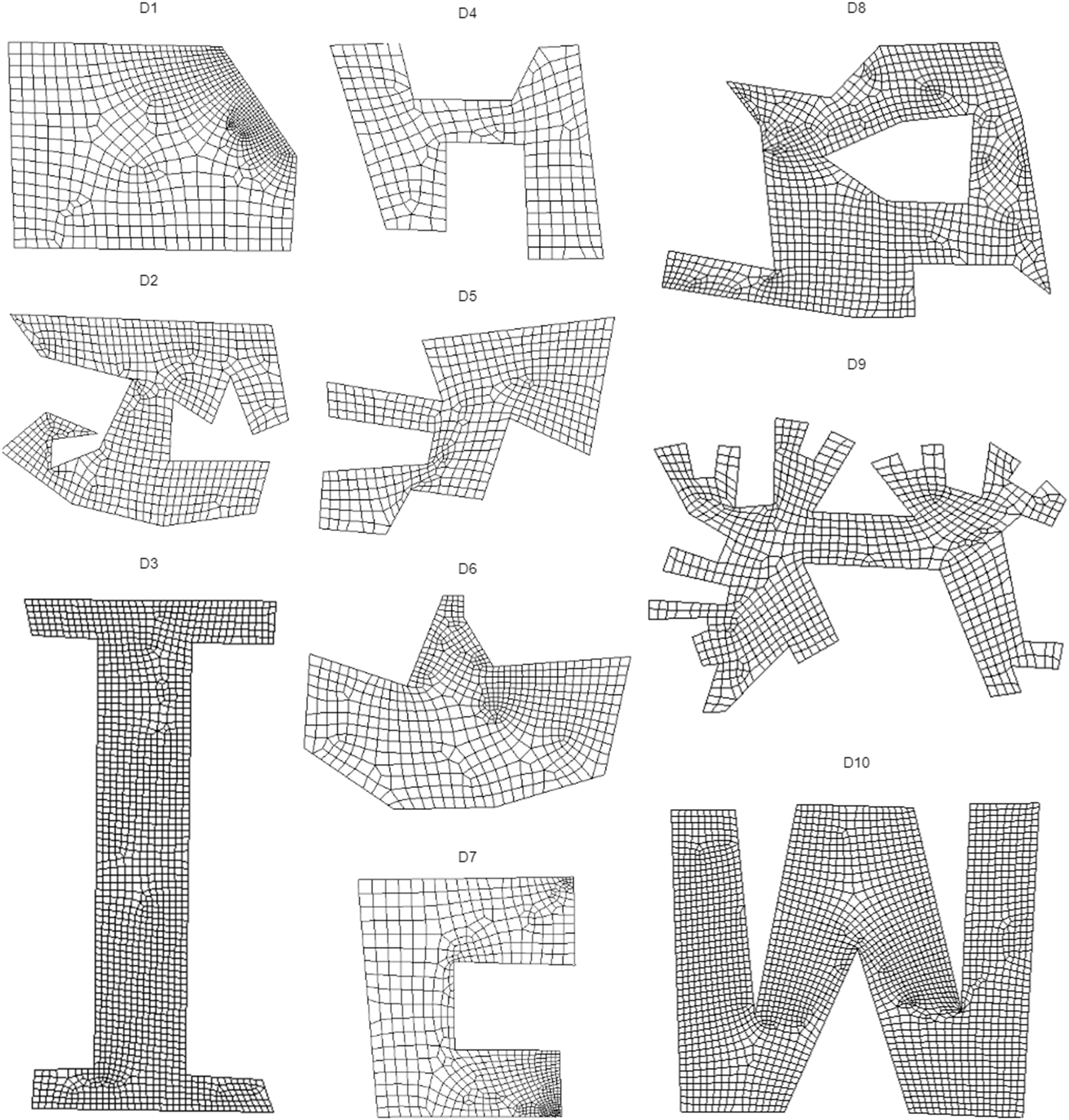
Fig. 26. All the meshing results of freeMesh-S.
Comparing results and analysis
All the meshing results of four methods, Gmsh-Blossom (GB), Gmsh-DelQuad (GD), and CUBIT-Pave (CP), and the proposed self-learning system FreeMesh-S (SS), on the ten experimental domains, are shown in Figures 27–29, and 21, respectively. All the domains have been successfully discretized into mesh elements, in which the methods CP and SS have more regular quadrilateral elements than GB and GD; and GD performs better than GB. The increase of meshes’ regularity can reduce computational consumption and improve the analysis results’ accuracy. GD and CP methods, however, cannot mesh all the domains into quadrilaterals. There are triangles in certain experimental domains, which require extra cleanup operations to eliminate them.
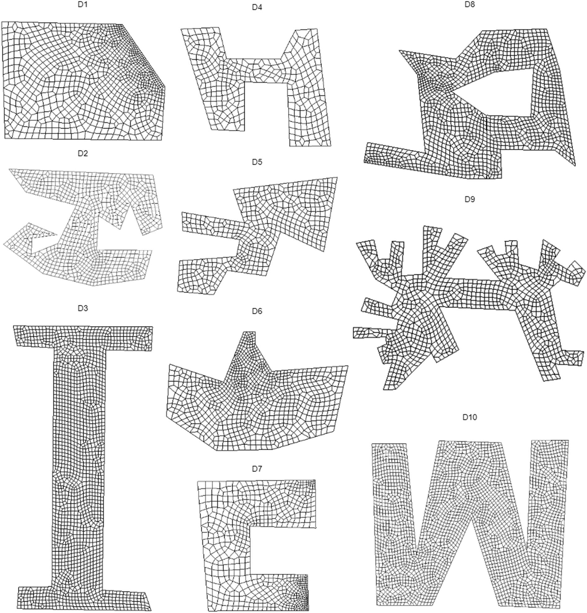
Fig. 27. Meshing results of GB method.
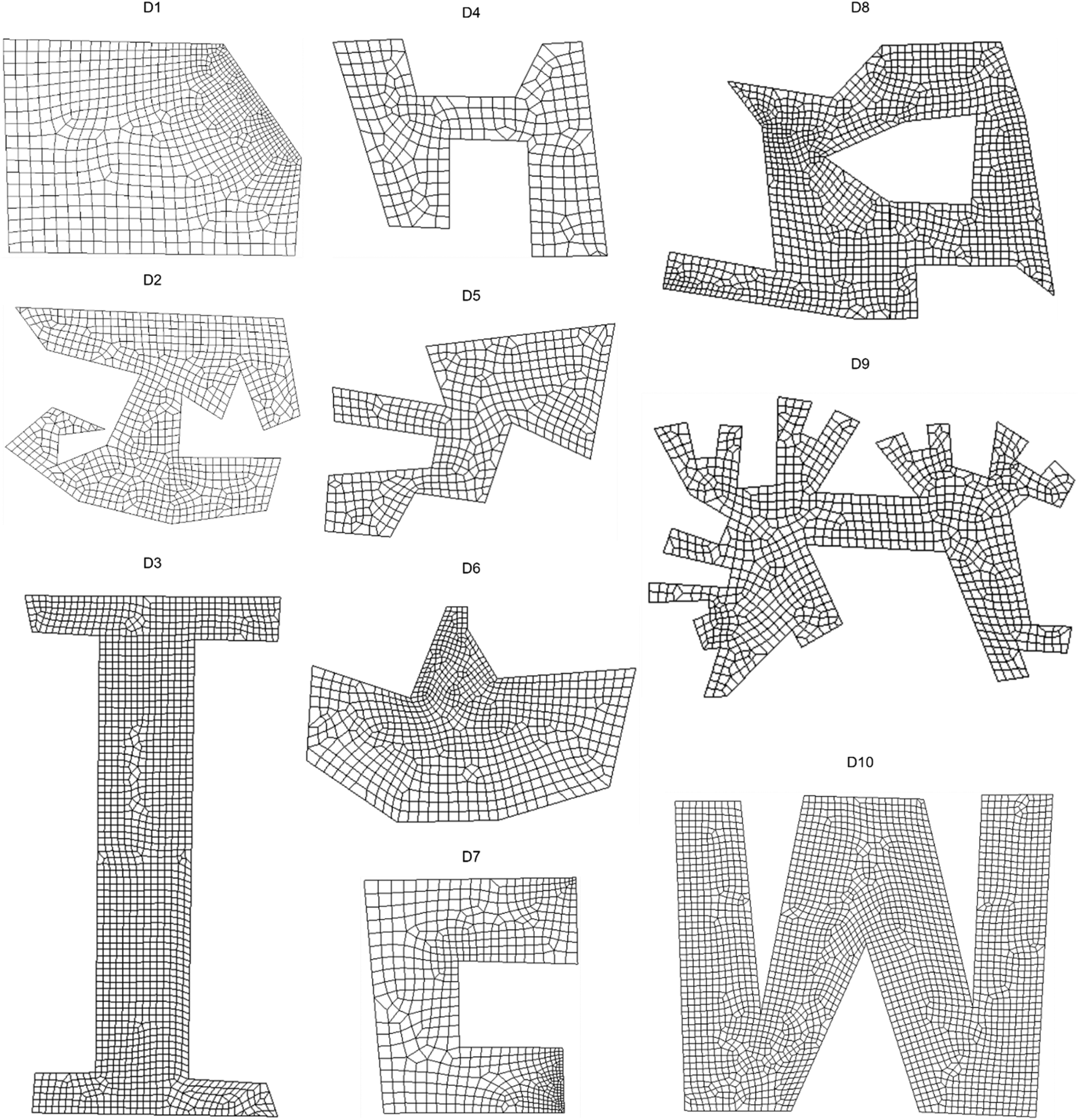
Fig. 28. Meshing results of GD method.
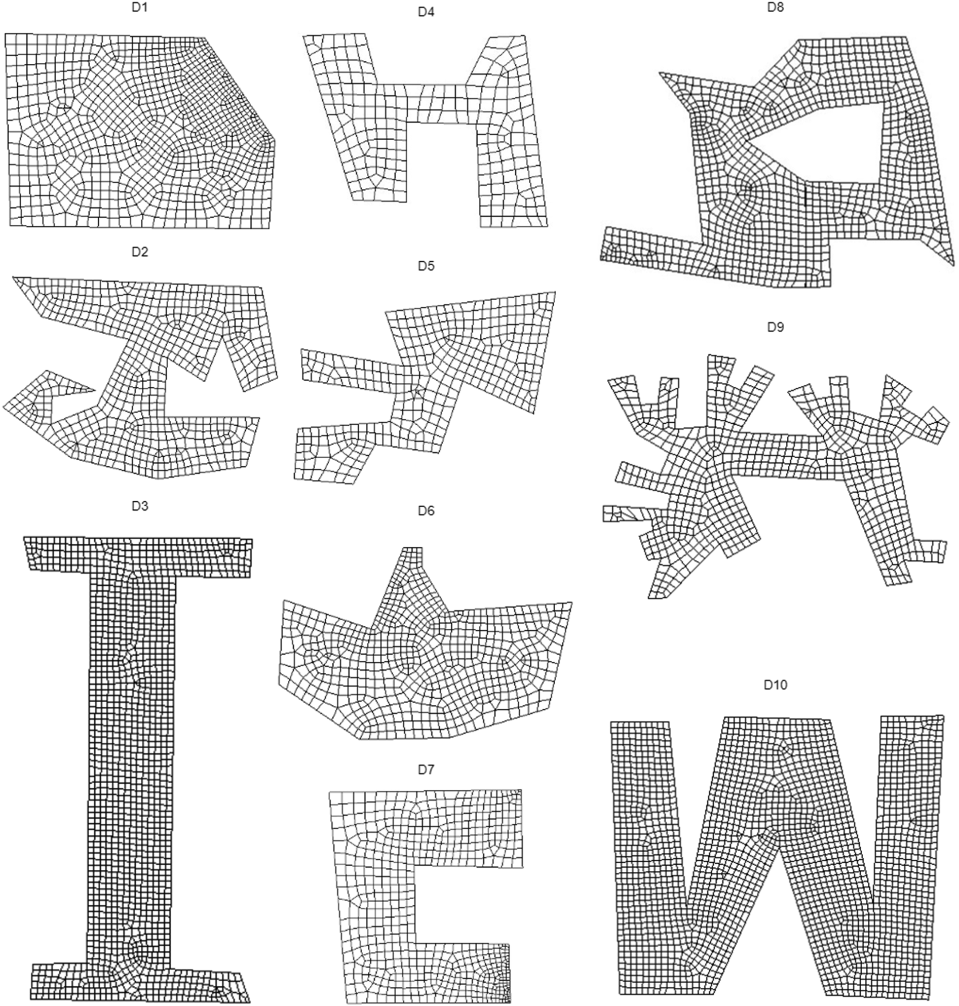
Fig. 29. Meshing results of CP method.
The statistics of the seven metrics are illustrated in Table 12 to measure the different performances of the four methods quantitatively. Each value in the table is the average over 10 domains (see detailed statistics in Table 10). The proposed SS method achieves the best performance in 2 quality metrics (Scaled Jacobian and Taper); CP method achieves the best performance in 5 quality metrics (Singularity, Element quality, Min angle, Max angle, and Scaled Jacobian); and GB is the best method from the aspect of Stretch. Moreover, the number of domains that each method achieves the best in each metric is shown in Figure 30. For each metric there are the following results.
• Singularity: Even though the CP method obtains the best-averaged performance against other methods, the self-learning system FreeMesh-S (SS) has very close results and excels in 2 domains when counting domains with best performances. GB and GD methods are less likely to handle the irregular vertices during meshing because of their dependence on triangulation. They cannot achieve good performance in all the domains. GD method, however, is better than GB because it conducts a pre-processing on the triangulation to make the triangular elements more suitable to be merged into quadrilaterals. Singularity impacts the numerical stability in CFD applications, wrinkles in subdivision surfaces, and breakdown of structured patterns on manifolds (Suresh and Verma, Reference Suresh and Verma2019).
• Element quality: FreeMesh-S (SS) resembles GD method and outperforms GB in this metric, while the CP method is the best one and excels in 7 domains. Nevertheless, SS is still comparable with other methods in the four domains. This measure is to identify how good a single element is, which can be calculated by Eq. (14).
• |Min/Max Angle - 90|: CP is better than the other three methods. FreeMesh-S (SS) has a similar performance with the GD method and outperforms GB. These two metrics show the difference between the minimal or maximum internal corners of an element and the degree of 90 because a square is considered the perfect element in quad meshing, that is, both of them are 90°.
• Scaled Jacobian: CP and SS have better results than the other two methods, while SS is slightly better than CP by excelling in 1 domain with the best performance. GB is the worst one. Scaled Jacobian relates to the interpolation error of finite element solution, for which the value of the best shape is 1.
• Stretch: GB is the best among the four methods and defeats all the methods in 10 domains. FreeMesh-S (SS) has a very similar performance with GD, while CP is slightly worse than the two methods by 0.01. Stretch is calculated by the ratio between the shortest edge and longest diagonal length, which indicates the degree of deformation.
• Taper: SS outperforms all the other methods and excels in 9 domains. Taper represents the ratio of the two triangles’ areas separated by a diagonal within a quadrilateral element, which indicates the balanced shape of an element.
Table 10. Mesh quality metrics of four methods on ten domains:L, H indicate if the lower value or higher value is preferred, respectively. The value in bold means the best among other approaches in a domain. GB refers to Gmsh-Blossom; GD indicates Gmsh-DelQuad; CP is CUBIT-Pave; and SS means the proposed self-learning system, FreeMesh-S


Fig. 30. Number of domains that each method achieves the best performance in each metrics.
In general, the proposed system, FreeMesh-S (SS), achieves high performance in all the metrics. All the values are within acceptable ranges as specified by the Verdict (Pébay et al., Reference Pébay, Thompson, Shepherd and Grosland2008) and outperform the other three approaches in Scaled Jacobian and Taper metrics. The CP approach has the best performance in Singularity, Element quality, |MinAngle - 90|, |MaxAngle - 90|, and Scaled Jacobian metrics. Even though almost losing all the competitions with other methods, the GB method has the best performance in the aspect of Stretch. The GD method exceeds the GB method in all the other metrics except the Stretch but is still poorer than SS and CP. GD is a quad-dominant method, which cannot discretize the whole domain into quadrilateral elements. Without extra cleanup operations (i.e., element deleting and insertion), CP and GD methods are challenging to generate a full-quad mesh. The proposed FreeMesh-S (SS) directly generates full-quadrilateral elements by the simulated extraction rules from A2C and FNN modules, which does not require any heuristic operations to handle exceptional triangle elements and inverted or flat quadrilateral elements.
Summary
The meshing performance of the proposed self-learning system is thoroughly evaluated by comparing it with the other three popular meshing approaches over ten complex domain boundaries. As been indicated in the introduction section, there is no single method that could perform the best in every measurement metric. This paper chooses seven commonly used indices to quantify meshing performance. The proposed FreeMesh-S achieves high in all of them and outperforms other methods in Scaled Jacobian and Taper metrics. FreeMesh-S also has a similar performance in Singularity with the best method – CP, which is suitable for applications needing regular meshes. Moreover, by analyzing the four methods’ computational efficiency, all of them have similar time complexity.
In the model training stage, the A2C shows that the agent can gradually generate good quality elements via trial-and-error learning, which is knowledge-free and needs no human intervention. The experience extraction module successfully extracts samples (i.e., input-output pairs) for the FNN training, which can turn several hundred elements into several hundred thousand samples. That is essential for the FNN model to get sufficient data and converge fast. The success of the combination of A2C and FNN demonstrates that the proposed self-learning schema is efficient in obtaining the extraction rules and sheds light on its applicability to other computational geometric problems.
Discussion
The proposed self-learning system, FreeMesh-S, has achieved high performance in meshing various complex domain boundaries compared to other meshing approaches, as illustrated in the previous experiment section. Furthermore, there are a few important implications of the proposed system from practical and theoretical system design perspectives.
Domain knowledge dependency
It requires researchers or developers to be equipped with equivalent knowledge for the selected method to develop an approach or mesh generation system. The mesh generation's lifecycle can be divided into four phases: pre-processing, element generation, quality measurement, and post-processing. The primary geometry knowledge required during the different development phases is shown in Table 11, respectively. For each stage, there are the following results:
• Pre-processing: Since the GB and GD are indirect methods to produce mesh elements, they need to generate triangulations in handling domains first. They need knowledge (e.g., Delaunay triangulation) to generate those triangles. GD intends to find ways to optimize the triangles to recombine them into high-quality quadrilateral elements. It requires, therefore, at least ten kinds of knowledge in the pre-processing phase; instead, the GB only needs Delaunay triangulation. CP and SS are direct quad meshing methods, which do not need any pre-processing operations.
• Element generation: GD and GB have a similar procedure to generate elements. The required knowledge for them is the same, including eight main categories. CP method requires less knowledge and needs four categories. SS needs the least knowledge to generate elements, which is also easy to understand.
• Quality measurement: All the approaches require two classes of knowledge. However, the required categories in SS, aspect, and taper ratio, are the simplest ones.
• Post-processing: GB and GD both need operations, including swapping the edges and removing the duplicated vertex in elements. GD also needs to smoothen the mesh using Lp Central Voronoi Tesselation (LPCVT) algorithm (Lévy and Liu, Reference Lévy and Liu2010). Moreover, GD is a quadrilateral-dominant method, which means that triangles may exist. CP method also requires geometrical operations, such as deleting and inserting elements and smoothing. SS does not involve any extra operations, and only needs smoothing, which is cleanup-free.
Table 11. Comparison of geometry knowledge required to develop and implement the algorithms and system

Table 12. Averaged mesh quality metrics of four methods on ten domains:L, H indicate if the lower value or higher value is preferred, respectively. The value in bold means the best among other approaches in a domain. GB refers to Gmsh-Blossom; GD indicates Gmsh-DelQuad; CP is CUBIT-Pave; and SS means the proposed self-learning system, FreeMesh-S

Generally, SS, being easy to understand, needs far less domain knowledge than others while maintaining promising meshing results. GD method has the most complicated geometry-related concepts to learn. GB is slightly less complex than GD in the pre-processing stage. Since CP and SS are direct meshing methods, they do not need any pre-processing knowledge. However, because CP relies on heuristic post-processing, it needs more knowledge in developing those cleanup operations. Therefore, SS is a development-friendly method for especially novice developers or researchers. This vital benefit makes it less knowledge-dependent in the method development and relieves humans from defining the input-output relations implied in the element extraction rules.
Designing a geometric algorithm is usually extremely difficult and time-consuming because the learning cost of geometric knowledge is high, especially for novel researchers. The self-learning and self-evolving FreeMesh-S system take two steps (i.e., defining the primitive rules and the self-learning process) in developing the algorithm, which smartly balances the human efforts and machine intelligence in the solution development.
The relation between smart design and smart system
The experiment found that the derived element extraction rules are applicable to 2D domains with almost any shape. The final obtained model can meshing domains with arbitrary boundaries without any additional training to fit their geometric specialty. Many existing meshing algorithms have difficulty in achieving high-quality elements in domains with sharp angles or restricted domains, such as one side of the geometric boundary (Rushdi et al., Reference Rushdi, Mitchell, Mahmoud, Bajaj and Ebeida2017). Even within a more regular geometric domain, they usually create flat or inverted elements that require heavy post-processing operations. It is challenging to guarantee that a method works on domains with arbitrary shapes while maintaining high quality. One of the most important properties of a smart system is that it can make adaptive decisions to maintain the system's overall performance. In the proposed FreeMesh-S system, the element extraction rules can be adaptive to various mesh boundaries. Three types of atomic rules were conceptually designed for the meshing problem through human intelligence, which is supported by a design methodology (Zeng and Cheng, Reference Zeng and Cheng1991; Zeng and Yao, Reference Zeng and Yao2009). This primitive property of the solution provides the foundation for smart applicability to arbitrary domains.
However, manually obtaining these rules is time-consuming and cannot meet the specified quality requirements. For example, human designers spend a lot of time observing various kinds of errors and come up with many heuristic operations such as element splitting, swapping, and collapsing to refine the overall mesh quality (Blacker and Stephenson, Reference Blacker and Stephenson1991; White and Kinney, Reference White and Kinney1997; Rushdi et al., Reference Rushdi, Mitchell, Mahmoud, Bajaj and Ebeida2017). Therefore, these rules should be smartly designed to be obtained automatically. It is also another important property of a smart system to self-evolve from trial-and-error. The proposed FreeMesh-S can automatically improve the extraction rules’ performance by integrating trial-and-error learning and supervised learning. The formed self-learning schema by A2C and FNN can quantitatively and automatically construct the atomic rules’ input-output relations without any human intervention.
In summary, the smart system can make adaptive decisions according to the external environment's changes and can be self-evolved from experiences. The smart design will greatly balance human efforts and machine intelligence and equip the system with these two properties. The FreeMesh-S has shed light on how to design such a smart system smartly and can be extended to other fields where the problem can be cast as recursive or atomic design problems.
Limitations
There are still a few limitations for the proposed self-learning system to resolve in the future. One challenge is that a domain with a very sharp angle is difficult to mesh. For example, a domain has a corner with a 1° angle. It is, however, a common problem for almost every meshing method (Shewchuk, Reference Shewchuk2012). The problem can be solved by cutting off the sharp corners or adding heuristic rules to form a quadrilateral element before applying the standard meshing method to the remaining boundary. The FreeMesh-S is also limited to mesh in single-connected domains. For a multi-connected domain (e.g., domain D9), the comprised solution taken by FreeMesh-S is to insert a cutting line to transform it into a single-connected domain, as shown in Figure 31. If there is more than one hole inside the domain, the same operation can be applied to each one of them.

Fig. 31. Multi-connected domain to single-connected domain. (1) multi-connected domain; (2) single-connected domain.
Conclusions
This paper aims to solve a challenging problem – learning from experience about the element extraction rules for achieving high-quality meshes in both the boundary and interior of complex geometric domains. Conventionally, to guarantee the overall mesh quality, element extraction methods rely heavily on heuristic operations, which is extremely difficult, expensive, and time-consuming for human algorithm designers. In this paper, a self-learning system FreeMesh-S is proposed to generate quadrilateral elements by automatically acquiring robust and high-quality element extraction rules. Firstly, according to the recursive logic, the extraction rules are categorized into three types (i.e., adding 1, 2, and 3 edges, respectively). A novel learning schema formed by A2C and FNN is then used to construct the input-output relations quantitatively and automatically. A2C simulates human trial-and-error learning to generate effective samples for training the three element-extraction rules using FNN. The experiment results demonstrate that derived element extraction rules can be adaptive to various boundary shapes and achieve high-performance quality metrics. Especially, the proposed method performs the best in Scaled Jacobian and Taper metrics, compared with the other three widely used meshing methods while requiring the minimal and most straightforward geometric knowledge.
Furthermore, this paper, for the first time, formulates the mesh generation problem as a Markov Decision Process (i.e., sequential decision making) problem. It closely bridges machine learning techniques with mesh generation and provides a smart way to balance the human efforts and machine intelligence in algorithm development, which could shed light on how to design a smart system smartly.
Acknowledgements
The support of the NSERC Discovery Grant is gratefully acknowledged.
Jie Pan is a PhD candidate at Concordia University. He received his B.S. from Southwest University of Science and Technology in 2013 and he received his M.E. in Huazhong University of Science and Technology in 2016. His research interests include mesh generation, reinforcement learning, learning system, and algorithm design. He specially focuses on building self-learning and self-evolving models for problems requiring sequential decision-making using reinforcement learning.
Jingwei Huang is a PhD in Information Engineering (University of Toronto, 2008), and an Associate Professor of Systems Engineering at Old Dominion University. He has extensive research experience applying artificial intelligence in systems engineering, cybersecurity and trust management. His previous work includes using logic-based AI approach for Knowledge Provenance ontologies, formal semantics of trust, trust calculus, trust mechanisms, trust models in PKIs, security policies integrating role-based and attribute-based access control models, and their applications in industry. Dr Huang's current research focuses on Digital Systems Engineering, to develop trustworthy AI/ML & Big Data solutions for Digital Engineering Transformation, and Data-Intensive Systems Modelling.
Yunli Wang is a Senior Research Officer at National Research Council Canada. She has proposed and developed machine learning algorithms to various problems in engineering, natural language processing, and bioinformatics. She received PhD from the Department of Precision Instrument, School of Mechanical Engineering of Tsinghua University in 2000 and Masters of Engineering from Northwestern Polytechnical University in 1997. She is an expert in the field of text mining and semi-supervised learning. She has published over 50 journal articles and peer-reviewed conference papers.
Gengdong Cheng is a professor in Department of Engineering Mechanics at Dalian University of Technology, Dalian, China. He is a Member of Chinese Academy of Sciences and a Foreign Member of Russian Academy of Sciences. He has authored or coauthored more than 200 articles in refereed journals, has translated two books, and has authored three books. His main research direction is computational mechanics, structural and multidisciplinary optimization.
Yong Zeng is a professor in Information Systems Engineering at Concordia University. He is the President of Society for Design and Process Science. He was NSERC Chair in aerospace design engineering (2015 - 2019) and Canada Research Chair in design science (2004 - 2014). Zeng researches into creative design by developing and employing mathematical and neurocognitive approaches. He has proposed Environment-Based Design (EBD) addressing the recursive nature of design and the role of mental stress in designer creativity. He applies the EBD to aerospace industry, medical device design, human resource management, municipality, teaching and learning design, and preventive medicine.