1. INTRODUCTION
Propagation of intense electromagnetic pulses in plasmas is a subject of current interest in a variety of areas that make use of the available modern laser technologies, among which we include particle and photon acceleration, nonlinear optics, laser fusion and other nonlinear processes. (Kozlov et al., Reference Kozlov, Litvak and Suvorov1979; Tajima & Dawson, Reference Tajima and Dawson1979; Mofiz & de Angelis, Reference Mofiz and de Angelis1985; Shukla et al., Reference Shukla, Rao, Yu and Tsintsadze1986; Esarey et al., Reference Esarey, Hafizi, Hubbard and Ting1998; Farina & Bulanov, Reference Farina and Bulanov2001; Mendonça, Reference Mendonça2001; Poornakala et al., Reference Poornakala, Das, Sen and Kaw2002; Bingham, Reference Bingham2003; Joshi & Katsouleas, Reference Joshi and Katsouleas2003).
Intense electromagnetic pulses displace plasma electrons and create a resulting ambipolar space-charge field with the associated density fluctuations. The ambipolar field here is known as the wakefield and can be used as an accelerating structure if stable and coherent enough that witnesses particles can absorb energy in a resonant fashion. Since the pulse couples with the wakefield, generation of the latter can affect the behavior of the former. Therefore, it is of interest to examine the coupled dynamics involving both fields.
This sort of investigation has been done in the literature. However, since focus has been mostly directed to fast pulses propagating nearly at the speed of light c, underdense plasma approximations are frequently used where the plasma frequency ωp is taken as small quantity. In this case, phase and group velocity are approximated by the speed of light (Duda & Mori, Reference Duda and Mori2000) and pulse distortions are either sometimes neglected, or treated under stationary wave assumptions (Bonatto et al., Reference Bonatto, Pakter and Rizzato2005).
A series of results of laser-plasma interactions are thus very specific to the underdense approximations, and our intention is therefore to examine how the system behaves when the approximation is relaxed. In particular, underdense approximations turn out to be too restrictive if one desires to follow the time dependent dynamics of laser pulses along the direction of modulation. In more specific terms, we shall investigate to what extent can an electromagnetic pulse retain its initial shape following its interaction with the wakefield, a relevant issue not only to accelerators but also to all sort of transmission of information using electromagnetic solitons (Gibbon, Reference Gibbon2007).
For a given pulse power, the dynamics is largely dictated by the pulse width. One of the findings here is that while wider pulses with widths sufficiently larger than the plasma wave length c/ωp may keep their shapes even in the presence of space-charge fields, narrow pulses with widths comparable to the plasma wavelength always tend to spread as time evolves. All depends ultimately on the pulse power and on relative roles played by relativistic and ponderomotive nonlinearities.
The paper is organized as follows. In Section 2, we define the relevant set of equations, in Section 3, we draw analytical estimates from approximate forms of the full theory identifying the regimes of interest, in Section 4, we compare estimates with full simulations, and in Section 5, we summarize and conclude the work.
2. THE MODEL
We initially follow previous works and the modulational formalism to reach the point we wish to discuss (Shukla et al., Reference Shukla, Rao, Yu and Tsintsadze1986; de Oliveira et al., Reference de Oliveira, Rizzato and Chian1995; Duda & Mori, Reference Duda and Mori2000).
Let us then consider our system as consisting of a mobile cold electronic fluid and a neutralizing fixed ionic background. We shall see that in terms of particle dynamics, even the smallest frequency scales analyzed in present model are on the order of the electron plasma frequency, which indeed allows to neglect ion motion.
All fields, radiation and wakes, propagate along the x axis of our coordinate system. The laser field is described by the associated vector potential A that takes the form
where A is the slowly varying complex amplitude of the field, with k0 and ω0, respectively, as the wavevector and frequency of the high-frequency carrier.
From the wave equation for the vector potential
and the equations of motion for the electron fluid that allows to write the current j in terms of the vector potential, one can write the governing equation for the weakly relativistic amplitude A (|qA/mc 2|≪1, with m and q as the electron mass and charge, respectively) in the form

where we have migrated to dimensionless quantities defined in the form ωpx/c → x, ωpt → t, qA/mc 2→A, and (n − n 0)/n 0 → n. n 0 is the equilibrium density, ωp = n 0q 2/ɛ0m denotes the plasma frequency, and μ0 and ɛ0 are the magnetic and electric vacuum permeabilities. We note that the frequency and wavevector of the carrier are normalized likewise.
On the right-hand-side of Eq. (3), one can devise the nonlinear features of the theory: the ponderomotive nonlinearity represented by the coupling involving density and vector potential, and the cubic relativistic nonlinearity which has its origins in the weakly relativistic expansion of the relativisitc factor γ.
Under the same set of approximations and normalizations, an equation for the slowly varying density fluctuations can be obtained in the form
where the term on the right-hand-side reflects the ponderomotive drive exciting the density wakefield.
We now proceed to reduce the equations into a simpler form, but taking care to avoid the occasional assumption used in underdense plasmas where the velocity of the laser pulse is approximated by the speed of light. We first of all note that in the slow modulational regime, it is convenient to introduce the wave frame coordinates τ = t and ξ = x − v gt where the group velocity of the radiation, v g, can be written as v g = k 0/ω0. If one moves to the new coordinates, and realizes that due to the slow modulations ∂/∂τ≪v g∂/∂ξ, and that without loss of generality the dimensionless dispersion relation ω02 = 1 + k 02 is obeyed, Eqs. (3) and (4) for laser and density fields take the form
Finally, we combine the nonlinear term |A|2/2 and the density field in Eqs. (5) and (6) into a new wakefield potential function φ ≡ v g2n − |A|2/2 (and define κ ≡ v g2 − 1) to write the final form of the dynamical equations

which is similar to derivations found in the literature (Shukla et al., Reference Shukla, Rao, Yu and Tsintsadze1986; Gibbon, 2007). We note that Eq. (8) governing the wakefield becomes time independent and no longer depends on derivatives of the laser pulse, which certainly helps to construct solutions for the problem. In addition, Eq. (7) now contains a cubic nonlinearity multiplied by the coefficient κ. In underdense approximations or in self-focusing studies, this term is occasionally neglected, but we shall see that its presence here is substantial to determine the dynamical regimes of the interaction.
All in all, the set (7) and (8) incarnates our basic model and shall now be the subject of our investigation.
3. INTEGRAL EXPRESSION FOR THE WAKEFIELD AND ANALYTICAL ESTIMATES
We first of all observe that since Eq. (8) is time independent, it can be integrated once the configuration of the laser pulse is given at any time, and proper boundary conditions are established. The proper boundary conditions results from the requirement that ahead of the pulse the wake is null, and the final expression for the wakefield can be written with help of Green's function as (Gibbon Reference Gibbon2007)
Eq. (9) shall be used in its full form in the coming simulations, but let us focus presently on two limits that can be examined.
3.1. Wide Pulses
The first case is the one where the width of the laser pulse — let us call it Δ — is much larger than the plasma wavelength c/ωp — in our dimensionless variables, Δ≪1. Under this condition the intensity |A(ξ)|2 varies slowly in Eq. (9) and integration by parts shows that φ → −|A|2/2 and n → 0, if one approximates ∂|A|2/∂ξ → 0. The wide pulse dynamics therefore turns out to be described by a nonlinear Schrödinger equation (NLS) of the form
Modeling the pulse as a Gaussian with time dependent amplitude and width, Lagrangian average methods (Duda & Mori, Reference Duda and Mori2000; Rizzato et al., Reference Rizzato, Oliveira and Chian2003; Nunes et al., Reference Nunes, Pakter, Rizzato, Endler and Souza2009) quickly reveal that under the present circumstances a stable pulse solution to Eq. (10) does exist, which can be found as the minimum of the effective potential U eff resulting from the method. The method generically allows to obtain an approximated dynamical equation for the pulse width Δ in the form
where in the wide pulse approximation U eff reads
W = ∫|A|2dx measuring the photon number within the pulse. κ < 0 and U effwide has exactly one minimum. One can write the equilibrium width Δw at the potential minimum of the stable pulse in the form
and the oscillatory frequency of slightly perturbed pulses around the minimum in the form
To illustrate for further purposes the general form of the wide pulse effective potential, the function U effwide is plotted in Figure 1 for v g2 = 0.99 and W = 0.01.

Fig. 1. U effwideversus Δ for v g2 = 0.99 and W = 0.01.
If Δw≫1 the stable solution is located in the wide pulse region and the wide pulse approximation should be expected to remain valid for all times if the initial condition lies sufficiently close to the stable solution and satisfies ![]() = 0. On the other hand, when Δw≲1, even if one starts with an initially wide pulse Δ (τ = 0) >1 the off-equilibrium pulse will drift toward the equilibrium Δw at the potential minimum. However, since the equilibrium now sits in a region where the wide pulse approximation does not hold, the fate of the pulse is uncertain and we shall resort to numerical simulations to investigate the dynamics there.
= 0. On the other hand, when Δw≲1, even if one starts with an initially wide pulse Δ (τ = 0) >1 the off-equilibrium pulse will drift toward the equilibrium Δw at the potential minimum. However, since the equilibrium now sits in a region where the wide pulse approximation does not hold, the fate of the pulse is uncertain and we shall resort to numerical simulations to investigate the dynamics there.
3.2. Narrow Pulses
Narrow pulses act like delta functions. Therefore φ ≈ 0 inside the pulse, although it can be large behind where it reads φ (ξ, τ) ≈ (1/2v g)W sin [(ξ − ξ0 (τ))/v g] with ξ0(τ) as the pulse position. Since φ → 0 inside the pulse, the full expression (7) can then be approximated by

Dispersive and nonlinear terms have opposite signs and the Lagrangian average method now reveals that regardless of the pulse power no static solution is to be found, with any pulse-like initial condition always spreading out as time evolves. The effective potential in this case reads

which indeed indicates that U effnarrow has no local minimum along the positive Δ axis. Since no fixed point is found here, the width grows until it reaches the transition region Δ ~ 1 where the approximation again fails and numerical work is once more required. U effwide is represented in Figure 2 for the same parameters of Figure 1.

Fig. 2. U effnarrowversus Δ for the same parameters of Figure 1.
To summarize, our estimates show the existence of a fixed point Δw only in the wide pulse approximation. If Δw≫1, the position of the fixed point is consistent with the approximation and any condition launched sufficiently close to the equilibrium will remain there. If Δw≲1 the fixed point is no longer consistent with the approximation. In this case, wide initial conditions will still drift toward Δw initially, but since the wide pulse approximation does not hold at Δ ~ Δw the pulse shall be accompanied numerically there.
On the other hand, the narrow pulse approximation does not offer any new fixed point. The respective effective potential clearly shows that any initial condition launched in the narrow pulse region always tends to move toward the wide region, across the transition region Δ ~ 1 where both approximations fail. Although the pulse initially behaves like a delta function, it is bound to reach the transition region where numerical analysis is again required.
4. COMPARING THE FULL SYSTEM AND ESTIMATES
With the previous estimates at our disposal, we now proceed to investigate the full system defined by Eqs. (7), and (8) or (9).
One particularly clear way to perform the analysis is through the construction of contour plots for the relevant fields. Let us do that for the laser intensity |A(ξ, τ)|2.
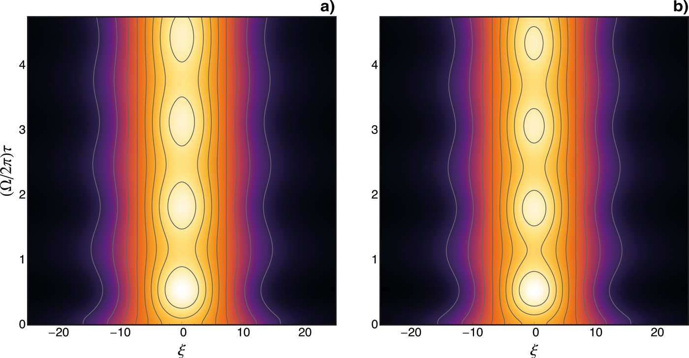
In Figure 3, we display the contour plots in the case where a fixed point can be found in the wide pulse region. Panel (a) depicts the approximation obtained from integration of the NLS equation, Eq. (10), and in panel (b) we plot the full solution to the set (7) and (9). We take the photon number as W = 0.01 with v g2 = 0.99. In that case, κ = 0.01 and Δw = 8, which indeed places the equilibrium solution in the wide pulse regime. As an initial condition, we launch a pulse with the shape of a hyperbolic secant of width Δ(τ = 0) = 10. It is important to note that in all cases numerically investigated in this paper, for each initial Δ, we start sitting precisely on top of the potential curves depicted either in Figure 1 or Figure 2; in this case, the initial momentum associated with the pulse expansion or contraction is null. Here one observes a nice agreement between the NLS approximation (10) and the full theory, with the pulse oscillating in a steady fashion around the equilibrium solution in both cases. The oscillatory frequency also agrees well with the value obtained from expression (14), at least for shorter times where radiation from the oscillating pulse is not yet significant.

Fig. 3. (Color online) Countour plots of |A(ξ, τ)|2 for W = 0.01, v g2 = 0.99 and Δ(0) = 10. In (a) the NLS wide approximation (10) and in (b) the full dynamics. The agreement is remarkable. In all countour plots, brighter shades correspond to higher amplitudes.
If we hold all the parameters unchanged, but now start from a narrow width Δ < 1, Δ(0) = 0.25, the case can be investigated with help of Figure 4. Comparision of the dynamics generated by the approximated NLS (15) as shown in panel (a), and by the full system (7) and (9) in panel (b), reveals that for short times the pulse starts opening up, as predicted by the narrow pulse approximation. For later times, panel (c) shows that the pulse crosses the transition region Δ ~ 1 mostly unhindered, and keeps opening up as it reaches and moves further into the wide region. The slight distortion of the full system, marginally seen in panel (c) as a leftward bending, takes place as the transition Δ ~ 1 is approached. It is actually a little surprising that the transition region should have only little effect on the pulse. But if one comes to think on the situation more carefully, as the pulse width reaches the transition, it is already opening up rapidly thanks to the fact that the initial condition sits on a much higher effective potential, as suggested by expression (16) for U effnarrow. As a consequence of the acquired “momentum,” or inertial dynamics, the pulse therefore gets across the transition essentially undeterred. As a rule that can be checked with further numerical discussion, the smaller the initial Δ, the smaller the pulse distortion as it crosses the transition; this agrees well with that view that smaller widths departs from higher effective potentials.
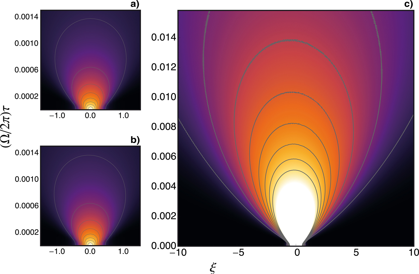
Fig. 4. (Color online) Contour plots of |A(ξ, τ)|2, again for W = 0.01 and v g2 = 0.99. All cases now depart from a narrow initial condition Δ(0) = 0.25. Panels (a) and (b) compare the NLS (10) and the full dynamics for short times. Panel (c) depicts the full dynamics for long times; notice the different time scale of (c) as compared to (a) and (b). Space on all horizontal axes, and time on vertical axes.
We next investigate the case where W = 0.1, keeping the previous value for v g. Now Δw ~ 0.8 < 1, which means that no stable solution exists in the wide region either. Pulses starting off wide configurations initially have their width reduced as commented earlier, but ultimately reach the transition region where are strongly affected by the wakefield as demonstrated in Figure 5. Panels (a) and (b) once again, respectively, refer to the NLS (10) and the full system for short times, while panel (c) depicts the full system for long enough times that allow the pulse reaches the transition region. In this case, the initial effective potential is not large enough to provide sufficient “momentum” with which the pulse could clear the transition region, and pulse distortion is thus appreciable.

Fig. 5. (Color online) Contour plots of |A(ξ, τ)|2 now for W = 0.1, keeping v g2 = 0.99. All cases depart from the wide initial condition Δ(0) = 10. As in the previous figure panels (a) and (b) compare the NLS (15) and the full dynamics for short times, and panel (c) depicts the full dynamics for long times.
Pulses starting off with a narrow configurations however have the same sort of behavior as in the previous case of a narrow initial condition. We start again from Δ(0) = 0.25 and the pulse simply keeps opening up, now with larger distortion as it traverses the transition region. The respective space-time history can be appreciated in the panels of Figure 6 — panel (a) now represents the short time, narrow pulse approximation provided by the NLS (15), panel (b) again represents the short time story of the full system, and panel (c) the long time story of the full system, where the pulse crosses the transition and submerge into the wide pulse region. For short times, full and approximated dynamics coincide, and at later times the more prominent distortion, as compared with that of Figure 4, results from the higher intensity wakefields generated here.

Fig. 6. (Color online) Contour plots of |A(ξ, τ)|2, again for W = 0.1 and v g2 = 0.99. All cases here depart from the narrow initial condition Δ(0) = 0.25. Once again panels (a) and (b) compare the NLS (15) and the full dynamics for short times, and panel (c) depicts the full dynamics for long times.
As a last view of the process, and to investigate issues related to pulse distortion in settings allowing all initial conditions to reach Δ ~ 1, in Figure 7, we display widths and spatial configuration of the laser squared amplitude |A|2 and wakefield φ at various instants of time, all for the case W = 0.1, v g2 = 0.99 when Δw lies within the transition region. In the upper row of panels, we represent full time evolution of the width Δ in (a), and a series of snapshots of the fields, (b) to (d), all for the initial condition Δ(0) = 10, away from the respective attracting transition region. In the lower row, we do the same for the narrow initial condition Δ(0) = 0.25 in (e) and (f) to (h), respectively.

Fig. 7. Widths and snapshots of field (| A(ξ, τ)|2 in solid lines, φ (ξ, τ) in dotted lines) evolution for W = 0.1, v g2 = 0.99. In the upper row of panels the initial condition reads Δ(0) = 10 (wide initial condition), and in the lower row, Δ(0) = 0.25 (narrow initial condition).
From the panels of Figure 7, once again one observes the asymmetry regarding the initial position at which the pulse is launched. Narrow pulses clear the transition and wider pulses are trapped and highly distorted there.
5. CONCLUSIONS
The present paper was devoted to the study of the coupled dynamics of laser pulses and wakefields in laser-plasmas systems.
Average Lagrangian methods have been employed to create estimates with which one can be guided in the investigation.
Briefly, restoring dimensions to the physical quantities, stable laser pulses were found in low power regimes where pulse width is much larger than the plasma wavelength, Δ≫c/ωp. In that case, estimates and full simulations of the coupled system agree to a large extent.
In cases of high power pulses, stable solutions are absent. Pulses initially launched from wide initial conditions shrink until it reach the transition region Δ ~ c/ωp where they are heavily distorted. On the other hand, pulses launched from narrow initial conditions Δ≪c/ωp traverse the transition region and keep spreading as they move deeper into the wide regimes. The asymmetry is credited to the fact that initially narrower pulses always depart from higher effective potentials, enabling the pulses to transverse the transition region Δ ~ c/ωp due to inertial effects.
If Δ ~ c/ωp, wakes are strongly excited. When narrow pulses traverse the transition region, wakes are briefly excited for as long as the pulse stays in the transition region. When the pulse comes from the wide pulse side and is allowed to reach the transition in higher power regimes such that Δw ~ c/ωp, it remains partially trapped there. Wakes are excited for longer stretches of time, albeit in an incoherent form.
We work with low power levels and neglect wavebreaking, which ought to be considered when |qA/mc 2| ~ 1. For such a large laser amplitude, fluid models must give way to PIC codes that deal directly with particle or kinetic models. The smaller amplitudes analyzed in this paper are however present in models and experiments (Gibbon, Reference Gibbon2007; Luttikhof et al., Reference Luttikhof, Khachatryan, van Goor, Boller and Mora2009), and the associated fluid models can certainly help to clarify the corresponding physics. Depending on pulse power and on how far from the transition region the initial conditions are launched, the modulational process described here may not be neglected. In the fastest cases considered in this work the time needed to produce appreciable distortion in the laser pulse ranges from 10–100 plasma periods, which indeed suggests an accurate description of the laser-wakefield self-consistent dynamics.
As a final comment on the subject of time scales, we note that our longest pulses satisfy (Δw/c)ωp = τpωp ~ 8 (τp = Δw/c is the pulse duration time) which is still short enough to preclude ion motion.
ACKNOWLEDGMENTS
We acknowledge support by CNPq, Brasil, and by the AFOSR, USA, grant FA9550-09-1-0283.