


1. INTRODUCTION
The “smart ship”, which can be defined as a vessel which can automatically collect data, assess its environment and make intelligent sailing decisions, is a future development trend in the shipping industry as it has the potential to lower risks to crew at sea, improve maritime traffic safety (Statheros et al., Reference Statheros, Howells and Maier2008; Wang, Reference Wang2010) and significantly reduce the costs to general manufacturing industry. Smart ships will be complicated and novel vessels which can detect their navigation surroundings autonomously and make sailing decisions without a human being's involvement (Burmeister et al., Reference Burmeister, Bruhn, Rødseth and Porathe2014; Statheros et al., Reference Statheros, Howells and Maier2008). Thus, it can be seen that the smart ship will remould the future operation modes of the shipping industry. Ship tracking is one of the critical technologies to facilatate the ability of smart ships to make sailing decisions and has attracted the attention of many researchers. Numerous studies have been completed which are relevant to the ship tracking topic, such as tracking and attacking intrusive ships (Gray et al., Reference Gray, Aouf, Richardson, Butters, Walmsley and Nicholls2011; Reference Gray, Aouf, Richardson, Butters and Walmsley2012; Han et al., Reference Han, Ra, Whang and Park2014), illegal fishing (Hu et al., Reference Hu, Yang and Huang2011), anti-piracy (Szpak and Tapamo, Reference Szpak and Tapamo2011) and so on. We do not list studies of ship tracking in darkness as our work does not cover this aspect.
Previous studies have shown that image processing-based methods can achieve satisfactory results in ship tracking. Ma et al. (Reference Ma, Shen and Wu2011) tried to find target ships in Vessel Traffic Services (VTS) videos with a Kalman filter algorithm. Considering ships recorded in videos with different viewpoints, Loomans et al. (Reference Loomans, de With and Wijnhoven2013) proposed an efficient object descriptor using a visual feature point tracker to carry out ship tracking tasks robustly. Teng et al. (Reference Teng, Liu, Gao and Zhu2013; Reference Teng, Liu and Zhu2014) and Teng and Liu (Reference Teng and Liu2014) conducted several studies to track ships sailing in inland waterways in real time. Some researchers have employed Automatic Identification System (AIS) and Synthetic Aperture Radar (SAR) technologies to track ships (Chaturvedi et al., Reference Chaturvedi, Yang, Ouchi and Shanmugam2012; Zhao et al., Reference Zhao, Ji, Xing, Zou and Zhou2014). From the perspective of traditional navigation, the above-mentioned ship tracking methods can sufficiently meet the ship-tracking demands of maritime safety administrations, ship owners, etc. In the smart ship era, crews will be smaller, resulting in challenges for the autonomous ship tracking task.
Firstly, the models used for ship tracking need to be very robust in varied environments, such as lighting variation, extreme weather, different viewpoints, etc. Conventional ship tracking methods may be ineffective in handling such challenges. For instance, SAR-based technologies have a degraded tracking performance under conditions of rain, snow and strong sea clutter. In addition, the disadvantage of AIS is that not all ships have been equipped with AIS, and ships at sea may deactivate their AIS transmitters (for example, warships, ships engaged in illegal activity, etc) (Xiao et al., Reference Xiao, Ligteringen, Van Gulijk and Ale2015; Zhang et al., Reference Zhang, Goerlandt, Montewka and Kujala2015; Reference Zhang, Goerlandt, Kujala and Wang2016; Reference Zhang, Kopca, Tang, Ma and Wang2017a). In such a situation, other techniques are required to help AIS-based methods track ships. Another ship tracking technique is Long Range Identification and Tracking (LRIT). Although the LRIT system provides accurate ship positions, it sends out ship information every six hours at best, far from all ships participate in LRIT, and LRIT data is seldom accessed by merchant ships but by shore authorities such as flag state, port or administration (Chen, Reference Chen2014). The data interval is too long for ship tracking in the smart ship era. Also, merchant ships may not be able to access LRIT data as the dataset is confidential (Lapinski et al., Reference Lapinski, Isenor and Webb2016; Vespe et al., Reference Vespe, Greidanus and Alvarez2015).
Secondly, ship video information (such as ship's imaging width and length) is crucial for a smart ship making sailing decisions. However, little attention has been paid to obtaining visual information in the existing ship tracking models. Thirdly, from the perspective of image processing, ship tracking in the smart ship era requires a higher accuracy compared to that in the traditional navigation era. Hence, efficient computer vision-based models are needed to assist in tackling the above-mentioned ship tracking challenges. We anticipate that a smart ship would employ both visual and non-visual tracking models to obtain a robust ship tracking performance.
Smart ships will require robust visual ship tracking methods to cope with different and challenging tracking situations. Several computer vision and machine learning methods have presented favourable results in the object tracking field (Joshi and Thakore, Reference Joshi and Thakore2012; Tang et al., Reference Tang, Liu, Zou, Zhang and Wang2017; Teng et al., Reference Teng, Liu, Gao and Zhu2013; Yan et al., Reference Yan, Zhang, Tang and Wang2017). Optical flow operators, Kalman trackers, Camshift and Meanshift descriptors are popular object tracking methods, which have shown their potential in ship tracking in smart ship applications (Allen et al., Reference Allen, Xu and Jin2004; Bardow et al., Reference Bardow, Davison and Leutenegger2016; Chauhan and Krishan, Reference Chauhan and Krishan2013; Tripathi et al., Reference Tripathi, Ghosh and Chandle2016). These methods track a target according to a target's single feature. The problem is that we cannot determine a universal single feature which can be applied in different tracking situations. Thus, these models may be inefficient in demanding ship-tracking situations (Tang et al., Reference Tang, Wang and Liu2013; Reference Tang, Zhang, Wang, Wang and Liu2015; Xu et al., Reference Xu, Tao and Xu2013; Zhang et al., Reference Zhang, Tang, Wang, Wang and An2017b).
Recently, multi-view learning-based methods have been proposed to solve the ineffectiveness of single-feature tracking methods. A bank of distinctive visual features, such as colour, intensity, edge and texture, are integrated into multi-view learning methods to achieve robust object tracking. Many studies have shown excellent tracking performance of multi-view methods (Delamarre and Faugeras, Reference Delamarre and Faugeras1999; Hong et al., Reference Hong, Mei, Prokhorov and Tao2013; Reference Hong, Chen, Wang, Mei, Prokhorov and Tao2015; Taj and Cavallaro, Reference Taj and Cavallaro2010). Impressed by the high performance of multi-view learning methods, a novel multi-view learning-based ship tracking framework is proposed in the context of smart ship applications. The proposed framework employs a multi-view learning method to explore intrinsic relationships between different unique ship-contour related features including Laplacian-of-Gaussian (LoG), Local Binary Patterns (LBP), Gabor, Histogram of Oriented Gradients (HOG) and Canny descriptors. A sparse representation method is then applied to represent mutual relations between the distinct features. Traditional powerful tracking methods, including Kalman and Meanshift trackers, have been implemented to verify the proposed methodology's efficiency and accuracy. Combining visual and traditional tracking methods can enhance maritime traffic safety considerably.
Our contributions can be summarised as follows. First, as there is no publicly accessible benchmark for evaluating ship trackers’ performance, we collected four typical video datasets for assessing different ship trackers’ performance. Second, we analysed bottlenecks existing in the visual ship tracking task. To solve this problem, we introduce a novel visual ship tracking framework based on a multi-view learning model and a sparse representation method. Third, the standard multi-view learning model employs appearance-based feature descriptors to obtain a robust tracking performance. Specifically, colour-related features play an important role in obtaining high tracking performance for conventional multi-view learning models. However, ships sailing in waterways often present similar or identical colours. Also, it is quite common for ships to have similar shapes. It is quite possible that a target ship has a similar appearance to its neighbours in tracking videos. Thus, the standard multi-view-based models, tracking through appearance-based feature sets, cannot deliver a satisfactory ship-tracking performance. However, it is worth noting that different ships possess unique textures and contours. Thus, we propose a novel ship tracking model based on a customised multi-view learning framework, which employs distinctive texture and contour-related features to complete the visual ship-tracking task.
2. METHODOLOGY FOR VISUAL SHIP TRACKING
2.1. Multi-view learning and sparse representation-based ship tracker
A ship tracking model needs to track ships in the Region Of Interest (ROI) with robust performance and low computational complexity. A Lasso regularisation (L1-norm)-based tracker, abbreviated as L1 tracker, is a popular object tracker, and it shows advantageous tracking accuracy with a short computation time (Friedman et al., Reference Friedman, Hastie and Tibshirani2008; Mei and Ling, Reference Mei and Ling2011). Hong et al. (Reference Hong, Mei, Prokhorov and Tao2013) pointed out that the L1 tracker may fail to track objects whose shape varies in tracking image sequences. Thus, a multi-view learning-based method was proposed to improve the L1 tracker's performance. Building on this work, we propose a novel ship tracking framework based on multi-view learning and a sparse representation method. The flowchart of our proposed ship tracker is shown in Figure 1.
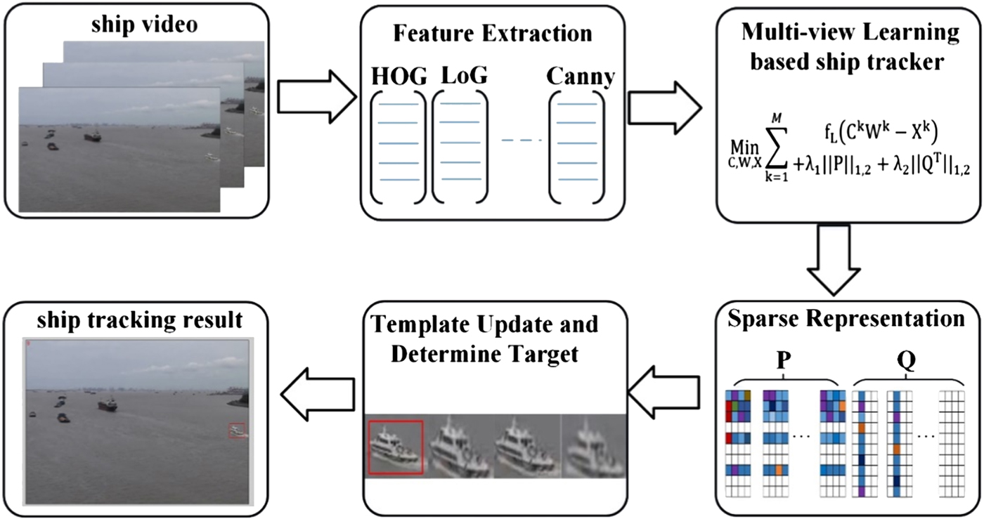
Figure 1. Workflow of the proposed ship tracker.
2.1.1. Feature extraction
Ships have clear contours and edges compared to water in videos. Hence, texture and structure-based feature descriptors are preferred for extracting ship features in the ROI. HOG and LoG descriptors are two useful texture descriptors which have shown success in many tracking tasks (Dalal and Triggs, Reference Dalal and Triggs2005; Gunn, Reference Gunn1999; Yang et al., Reference Yang, Liang and Jia2012). Details of obtaining a HOG descriptor can be found in Dalal and Triggs (Reference Dalal and Triggs2005) and Suard et al. (Reference Suard, Rakotomamonjy, Bensrhair and Broggi2006). The LoG descriptor is a popular blob-detector method (Silvas et al., Reference Silvas, Hereijgers, Peng, Hofman and Steinbuch2016), which suits well for visual ship tracking tasks. The LBP descriptor possesses features of rotation and brightness invariance. These two feature descriptors are scale-invariant and are very useful for tracking target ships that show a varied appearance in surveillance videos. The Gabor descriptor is insensitive to illumination variance, and we employ a Two-Dimensional (2D) Gabor filter as another distinct ship edge descriptor. More details can be found in Sun et al. (Reference Sun, Bebis and Miller2005). A Canny descriptor is a ladder-shaped edge detector which is sensitive in detecting ship edge variation (Canny, Reference Canny1986). The proposed ship tracker extracts these five distinct edge descriptors and integrates them into a coupled ship tracking descriptor. In the following section, we use symbol M, instead of five, to indicate the number of views in our proposed multi-view learning model.
2.1.2. Robust Ship Tracker based on Multi-view learning and Sparse representation (STMS)
2.1.2.1. Ship tracking model by multi-view learning and sparse representation
Hong et al. (Reference Hong, Mei, Prokhorov and Tao2013) and Mei et al. (Reference Mei, Hong, Prokhorov and Tao2015) proposed a generative multi-view learning-based tracker which showed impressive tracking performance. However the tracker proposed by Hong et al. (Reference Hong, Mei, Prokhorov and Tao2013) cannot be used to perform the visual ship tracking task directly. The reason is that the to-be-tracked features in the Hong-proposed tracker are of a colour and intensity which may be quite similar among different ships. Thus, the Hong-proposed tracker is prone to fail in the visual ship tracking task. To address this problem, we propose a robust multi-view learning and sparse representation-based ship tracker.
For a view k in the STMS model, we denote Ck as a complete ship dictionary, and Xk is the corresponding feature matrix. The representation matrix for Ck is demonstrated as Wk. Our tracker solves the ship tracking problem by finding the minimum value of Equation (1). The product of the complete dictionary and feature matrix of M views ( $\sum\nolimits_{{\rm k} = 1}^{\rm M} {{\rm C}^{\rm k}{\rm W}^{\rm k}} $ in Equation (1)) represents a potential ship target. fL(Ck Wk − Xk) (k = 1, 2, … M) is a cost function of evaluating the vessel reconstruction error between the ship candidate and ship template regarding the kth view. A smaller value of the cost function fL( Ck Wk − Xk) means better tracking performance. Hence, the optimal tracking performance of our tracker is obtained when we find the minimum value of Equation (1).
We introduce a sparse representation method to find a robust solution for Equation (1) more efficiently. We decompose the representation matrix Wk (k = 1, 2… M) as coefficient matrix Pk and Qk (see Equation (2)). Pk is the representation matrix for the kth view. Global representation matrix P (similar to Q) is acquired by padding Pk s (k = 1, 2… M) horizontally. The STMS model of Equation (1) is then rewritten as Equation (3). As the dictionary Ck is an over-complete dictionary in the kth view of Equation (3), more elements in Pk and Qk will better explore the intrinsic relationship between the M-views. Hence, the discrepancy between the ship candidate's feature Ck(Pk + Qk) and the extracted feature Xk will become smaller. A higher order of P and Q will lead to better tracking accuracy in terms of the cost function in Equation (3).
However, a higher order for the coefficient matrices P and Q results in higher complexity for our tracker. So, the method of group Least Absolute Shrinkage and Selection Operator (LASSO) penalty, denoted as ℓ1, 2, is introduced to reduce the tracker's complexity. Parameter ||P||1, 2 represents the independence of each view and is constrained via row sparse representation through the ℓ1, 2 method. The constraint of the row sparse representation for the matrix P helps our tracker explore latent relationships between different views, and a stronger relationship will lead to a lower order of P. Meanwhile, the lower order of P indicates that P is a lower-order sparsity matrix. Parameters λ1 in Equation (3) control the sparsity of the coefficient matrix of P. The term  $\lambda _1\left\| P \right\|_{1,2}$ reduces the order of P to a minimum level in the procedure of finding the optimal solution in Equation (3).
 $\left\| {{\rm Q}^{\rm T}} \right\|_{1,2}$ in Equation (3) represents the abnormal tracking results which are subjected to a group LASSO penalty, and λ2 is a sparse coefficient of Q. A smaller order for Q means that the tracking results have fewer outliers. Thus, fewer elements in the over-complete dictionary will be employed in the proposed ship tracker. In summary, lower orders for P and Q represent smaller values for the term of
  $\lambda _1\left\| {\rm P} \right\|_{1,2} + \lambda _2\left\| {{\rm Q}^{\rm T}} \right\|_{1,2}$, which leads to a better solution for Equation (3). Based on the above discussions about the constraints on the sparse matrices P and Q, we can conclude that our proposed ship tracker can find the optimal tracking result by solving Equation (3). Previous studies have shown that high performance is obtained by substituting the cost function in Equation (3) with the Frobenius norm (Mei et al., Reference Mei, Hong, Prokhorov and Tao2015). The Frobenius norm is denoted as
  $\left\| \bullet \right\|_F^2 $. Therefore, our tracker can be reformulated to Equation (4).
 $$\mathop {\hbox{Min}}\limits_{{\rm c},{\rm w},{\rm x}} \sum\limits_{{\rm k} = 1}^{\rm M} {\hbox{f}_{\rm L}} \lpar {\hbox{C}^{\rm k}\hbox{W}^{\rm k} - \hbox{X}^{\rm k}} \rpar $$
 $$\hbox{W}^{\rm k}=\hbox{P}^{\rm k}+\hbox{Q}^{\rm k}\quad k=1,2\ldots M$$
 $$\mathop {\hbox{Min}}\limits_{{\rm c},{\rm w},{\rm x}} \sum\limits_{{\rm k} = 1}^M {\hbox{f}_{\rm L}} \lpar {\hbox{C}^{\rm k}\hbox{W}^{\rm k} - \hbox{X}^{\rm k}} \rpar + \lambda _1{\rm \Vert }\hbox{P}{\rm \Vert }_{1,2} + \lambda _2{\rm \Vert }\hbox{Q}^{\rm T}{\rm \Vert }_{1,2}$$
 $$\mathop {\hbox{Min}}\limits_{{\rm c},{\rm w},{\rm x}} \sum\limits_{{\rm k} = 1}^{\rm M} {\displaystyle{1 \over 2}} {\rm \Vert }\hbox{C}^{\rm k}\hbox{W}^{\rm k} - \hbox{X}^{\rm k}{\rm \Vert }_{\rm F}^2 + \lambda _1{\rm \Vert }\hbox{P}{\rm \Vert }_{1,2} + \lambda _2{\rm \Vert }\hbox{Q}^{\rm T}{\rm \Vert }_{1,2}$$
2.1.2.2. Optimal solution for STMS model
The tracking performance of the STMS model largely depends on the solution of Equation (4). For the sake of simplicity, we rewrite Equation (4) into two parts as shown in Equations (5) and (6), respectively. So, solutions for Equations (5) and (6) represent the potential tracking target. The Accelerated Proximal Gradient (APG) method is efficient in solving Frobenius-norm based problems (Zhang et al., Reference Zhang, Ghanem, Liu and Ahuja2012). In fact, the APG method acquires  ${\rm O}\left( {{\textstyle{1 \over {{\rm m}^2}}}} \right)$ residual of the optimal solution at the mth iteration. Hence, we employ an APG algorithm to solve Equations (5) and (6). The APG algorithm finds an optimal solution for Equation (4) through two steps: composite gradient mapping and aggregation.
 $$\hbox{s}\lpar {\hbox{P},\hbox{Q}} \rpar = \sum\limits_{{\rm k} = 1}^{\rm M} {\displaystyle{1 \over 2}} {\rm \Vert }\hbox{C}^{\rm k}\hbox{W}^{\rm k} - \hbox{X}^{\rm k}{\rm \Vert }_{\rm F}^2$$
 $${\rm r(P},{\rm Q)} = \lambda _1\left\| {\rm P} \right\|_{1,2} + \lambda _2\left\| {{\rm Q}^{\rm T}} \right\|_{1,2}$$
Step 1: Composite Gradient Mapping. Inspired by Gong et al. (Reference Gong, Ye and Zhang2012) and Hong et al. (Reference Hong, Mei, Prokhorov and Tao2013), we apply a composite gradient mapping algorithm to address Equation (4). Thus, based on Equations (5) and (6), Equation (4) can be reformulated as Equation (7). In Equation (7), s(U, V) is the value of s(P, Q) at point (U, V) and s(U, V) is estimated by the first order of the corresponding Taylor expansion. Parameter r(P, Q) in Ω(P, Q; U, V) is a regularised factor. We employ the squared Euclidean distance between (P, Q) and (R, S) to represent the regularisation term.
 $$\eqalign{\Omega (\hbox{P},\hbox{Q};\hbox{U},\hbox{V}) =& \hbox{s}(\hbox{U},\hbox{V}) + \langle \nabla _{\rm U}\hbox{s}(\hbox{U},\hbox{V}),\hbox{P} - \hbox{U}\rangle + \langle \nabla _{\rm V}\hbox{s}(\hbox{U},\hbox{V}),\hbox{Q} - \hbox{V}\rangle \cr & + \displaystyle{\sigma \over 2}{\rm \Vert }\hbox{P} - \hbox{U}{\rm \Vert }_{\rm F}^2 + \displaystyle{\sigma \over 2}{\rm \Vert }\hbox{Q} - \hbox{V}{\rm \Vert }_{\rm F}^2 + \hbox{r}(\hbox{P},\hbox{Q})}$$
 where  $\nabla_{\rm U}\hbox{s}(\hbox{U},\hbox{V})$ and
  $\nabla_{\rm V}\hbox{s}(\hbox{U},\hbox{V})$ are partial derivatives of s(U, V) for U and V respectively. The term
  $\langle\nabla_{\rm U}\hbox{s}(\hbox{U},\hbox{V}),\hbox{P}-\hbox{U}\rangle$ is the inner product of
  $\nabla_{\rm U}\hbox{s}(\hbox{U},\hbox{V})$ and P− U. Also, parameter
  $\langle\nabla_{\rm U}\hbox{s}(\hbox{U},\hbox{V}),\hbox{Q}-\hbox{V}\rangle$ is the inner product of
  $\nabla_{\rm V}\hbox{s}(\hbox{U},\hbox{V})$ and Q− V. Parameter σ is a penalty parameter.
Step 2: Aggregation. For the mth APG iteration process, (Um+1, Vm+1) is obtained through a linear combination of (Pm, Qm) and (Pm−1, Qm−1). Thus, we can update (Um+1, Vm+1) with Equations (8) and (9) which is termed as the aggregation step. The parameter βm is obtained by Equation (10).
 $${\rm U}^{{\rm m} + 1} = {\rm P}^{\rm m} + {\rm \beta }_{\rm m}\left( {\displaystyle{1 \over {{\rm \beta }_{{\rm m} - 1}}} - 1} \right)({\rm P}^{\rm m} - {\rm P}^{{\rm m} - 1})$$
 $${\rm V}^{{\rm m} + 1} = {\rm Q}^{\rm m} + {\rm \beta }_{\rm m}\left( {\displaystyle{1 \over {{\rm \beta }_{{\rm m} - 1}}} - 1} \right)({\rm Q}^{\rm m} - {\rm Q}^{{\rm m} - 1})$$
 $${\rm \beta }_{\rm m} = \left\{ {\matrix{ {\displaystyle{2 \over {{\rm m} + 3}}} \hfill & {m > 0} \hfill \cr 1 \hfill & {{\rm m} = 0} \hfill \cr } } \right.$$
P0, Q0, U1, V1 are set to zero for initialisation.
Given an aggregation point (Um, Vm), the solution for the mth APG iteration process is obtained by solving Equation (11). The minimisation Equation (11) is reformulated as finding optimal solutions for Pm and Qm in Equations (12) and (13). According to Hong et al. (Reference Hong, Mei, Prokhorov and Tao2013) there is an efficient close-form solution for obtaining an optimal Pm and Qm. Equations (14) and (15) present final solutions for Pm and Qm, respectively. In Equation (14),  ${\rm P}_{{\rm i.,}}^{\rm m} $ is the ith row of Pm, and
  ${\rm Q}_{{\rm .,j}}^{\rm m} $ in Equation (15) is the jth column for Qm.
  ${\rm U}_{{\rm i,.}}^{\rm m} $ is the ith row of Um and
  ${\rm V}_{{\rm .,j}}^{\rm m} $ is the jth column of Vm. We obtain P and Q by computing Equations (14) and (15) iteratively. Our proposed ship tracker determines the final tracked ship based on the final solutions of Equations (14) and (15). The symbol
  $\left\| \bullet \right\|$ in Equation (14) and (15) represents the Euclidean distance.
 $$(\hbox{P}^{\rm m},\hbox{Q}^{\rm m})=\hbox{arg}_{\rm P,Q}\min \Omega (\hbox{P},\hbox{Q};\hbox{U}^{\rm m},\hbox{V}^{\rm m})$$
 $$\hbox{P}^{\rm m} = \hbox{arg}{\mkern 1mu} \mathop {\hbox{Min}}\limits_P \displaystyle{1 \over 2}{\rm \Vert }\hbox{P} - (\hbox{U}^{\rm m} - \displaystyle{1 \over \sigma }\nabla _{\rm U}\hbox{s}(\hbox{U}^{\rm m},\hbox{V}^{\rm m})){\rm \Vert }_{\rm F}^2 + \displaystyle{{\lambda _1} \over \sigma }{\rm \Vert }\hbox{P}{\rm \Vert }_{1,2}$$
 $${\rm Q}^{\rm m} = {\rm arg}\mathop {{\rm Min}}\limits_Q \displaystyle{1 \over 2}\left\| {{\rm Q} - \left( {{\rm V}^{\rm m} - \displaystyle{1 \over \sigma }\nabla _V{\rm s}({\rm U}^{\rm m},{\rm V}^{\rm m})} \right)_F^2 } \right\|_F^2 + \displaystyle{{\lambda _2} \over \sigma }{\rm \Vert }{\rm Q}^{\rm T}{\rm \Vert }_{1,2}$$
 $$\hbox{P}_{{\rm i},.}^{\rm m} = \max \left( {0,1 - \displaystyle{{\lambda_1} \over {{\rm \Vert }\sigma \hbox{U}_{{\rm i},.}^{\rm m} - \nabla_{\rm U}\hbox{s}(\hbox{U}_{{\rm i},.}^{\rm m} ,\hbox{V}^{\rm m}){\rm \Vert }}}} \right)\hbox{U}_{{\rm i},.}^{\rm m}$$
 $$\hbox{Q}_{.,{\rm j}}^{\rm m} = \max \left( {0,1 - \displaystyle{{\lambda_2} \over {{\rm \Vert }\sigma \hbox{V}_{.,{\rm i}}^{\rm m} - \nabla_{\rm V}\hbox{s}(\hbox{U}^{\rm m},\hbox{V}_{.,{\rm i}}^{\rm m} ){\rm \Vert }}}} \right)\hbox{V}_{.,{\rm j}}^{\rm m}$$
3. EXPERIMENTS AND RESULTS
3.1. Data
Currently, there are few ship video datasets available for evaluating visual ship trackers’ performance. Hence, it is necessary to establish a benchmark of ship videos. To this end, we have taken maritime surveillance videos of four common scenarios at Shanghai Port. The collected videos for the four scenarios are denoted as Case-1, Case-2, Case-3 and Case-4. It is known that ripples and wakes impose strong interference on ship tracking models, so Case-1 aims to test the ship tracker's robustness within the constraints.
Another challenge is ship-overlapping in the image sequences, and we collected two videos to evaluate the ship tracker's performance under such a situation. Specifically, Case-2 is a video in which a to-be-tracked ship shows a different appearance (that is, colour and shapes, etc.) from the neighbouring ships. In the other video (that is, Case-3), the to-be-tracked ship has a similar appearance to its neighbours. Case-4 is to assess a tracker's performance in a tracking situation where the to-be-tracked ship is in the distance. To visualise a ship tracker's performance, we have manually labelled the Target Region (TR), in the form of a rectangle, in each frame of the four datasets. The TR rectangle is stored with the information of x-coordinate and y-coordinate of its upper-left vertex, width and height. Ship videos and TR sequences of the above four cases are available from the correspondence e-mail address. As these four cases are common situations in ship tracking applications, they can assist in adequately assessing and evaluating a ship tracker's performance. Samples of the collected videos for each case are shown in Figure 2.

Figure 2. Samples of collected datasets for each case (the TR is encircled with red rectangle in each image).
3.2. Evaluation criteria
To evaluate our ship tracker's performance, we compared the tracking results with the manually labelled TR rectangles in the collected videos. Tracking results are stored in the same data format as TR rectangles. For simplicity, both the TR rectangle and the tracked ship rectangle are denoted by their centre point (that is, the Intersection Point (IP) of a rectangle's diagonals). Based on that, we compare the distance of centre points between the tracked and TR rectangles to quantify a ship tracker's performance.
Two statistical indicators are used to demonstrate a ship tracker's performance, which are Mean Square Error (MSE) and Mean Absolute Difference (MAD). For a given video with n-frames, we denote GIP(x, y) as the IP coordinate of a rectangle in the TR sequences. TIP(x, y) is the centre point of the tracked rectangle. Here, the square root is denoted by symbol  $\left\| \bullet \right\|^{{\textstyle{1 \over 2}}}$ and a quadratic operator is denoted by
  $\left\| \bullet \right\|^2$. So, the offset between the tracked ship-rectangle and the TR rectangle is measured by the distance between GIP(x, y) and TIP(x, y) (see Equation (16)). Parameter Dt(x) represents the squared distance, in the x-axis, between GIP(x, y) and TIP(x, y) of the tth frame. Similarly, Dt( y) represents the squared distance in the y-axis. Parameters Dt( x) and Dt( y) are obtained by Equations (17) and (18), respectively.
After obtaining the distance in Equation (16), a ship tracker's performance is measured by the statistical indicators MSE and MAD (see Equations (19) and (20)). Parameter  $\bar{D}$ in Equation (19) is the average Euclidean distance. Equation (21) presents the calculation process for
  $\bar{D}$. Smaller values of MSE and MAD show better tracking performance for the ship tracker.
 $$D_t({\rm G}_{IP}(x,y),{\rm T}_{IP}(x,y)) = {\rm \Vert }{\rm D}_t({\rm x}) + {\rm D}_t({\rm y}){\rm \Vert }^{{\textstyle{1 \over 2}}}$$
 $${\rm D}_t({\rm x}) = \left\| {G_{IP}^t (x) - T_{IP}^t (x)} \right\|^2$$
 $${\rm D}_t({\rm y}) = \left\| {G_{IP}^t (y) - T_{IP}^t (y)} \right\|^2$$
 $$MSE = \left\| {\displaystyle{{\sum\nolimits_{t = 1}^n {{\rm \Vert }D_t(G_{IP}(x,y),{\rm T}_{IP}(x,y)) - \bar D{\rm \Vert }^2} } \over n}} \right\|^{\displaystyle{1 \over 2}}$$
 $$MAD = \displaystyle{{\sum\nolimits_{t = 1}^n {|D_t({\rm G}_{IP}(x,y),{\rm T}_{IP}(x,y)) - \bar D|} } \over n}$$
 $$\bar D = \displaystyle{{\sum\nolimits_{t = 1}^n {D_t} ({\rm G}_{IP}(x,y),{\rm T}_{IP}(x,y))} \over n}$$
3.3. Experiment setup and results
To evaluate our tracker's performance, two classical tracking algorithms, a basic Kalman tracker (Welch and Bishop, Reference Welch and Bishop1995) and a Meanshift tracker (Comaniciu et al., Reference Comaniciu, Ramesh and Meer2000), were implemented on the collected datasets. All trackers were executed on the Windows 10 Operation System PC with 8GB RAM and a 3·4 GHz CPU. Meanwhile, these models were built through Matlab (R2011 version) and a c++ library. The TR locations of the first frame in the four datasets were used to initialise ROI for the three trackers.
3.3.1. Tracking results for Case-1
All three trackers have been tested on the Case-1 dataset to present their robustness against ripple interference. It is clearly shown in Table 1 that our proposed ship tracker was better than other trackers. Specifically, MSE for the Kalman tracker was six times larger than that of the Meanshift tracker. Meanwhile, the MSE obtained by the Meanshift tracker was almost eight times larger than the STMS model. In sum, the STMS model could track a ship successfully in terms of MSE, while the Kalman tracker was the worst tracker under Case-1. The minimum statistical tracking errors of MSE and MAD were 3·6 and 2·8 pixels, respectively. Both of these were obtained by the STMS model. Based on the tracking errors, denoted by MSE and MAD, it is reasonable to conclude that our proposed ship tracker is more robust to ripple interference when compared to the other two trackers.
Table 1. Statistical performance of different ship trackers for Case-1.

Figure 3(a) shows the distance between the Tracked IP and TR's IP (TTRIP). In order to better visualise the distance variation for Case-1, the maximum value of TTRIP was set to 200 pixels. The distance distribution showed that the Kalman tracker was vulnerable to ripple interference. It is observed that the TTRIP, obtained by the Kalman tracker, increased significantly with the increase of tracking sequences, arriving at the maximum value at the 80th frame for the first time. Although the TTRIP fluctuated significantly in the subsequent 30 frames, it stayed at a maximum value from the 110th frame.

Figure 3. Distance distribution of TTRIP for the three trackers in each case.
In contrast, both the Meanshift and STMS trackers obtained a smaller TTRIP than that of the Kalman tracker as shown in Figure 3(a). In the first 350 frames, the Meanshift and STMS models had similar tracking result as the TTRIPs were quite close to each other. However, the TTRIP of the Meanshift tracker increased dramatically in the last 130 frames while STMS maintained a small value. After carefully checking the initial tracking video, we found that the target ship became smaller in the later frames. So, some ripples were tracked by the Meanshift tracker. As ripples randomly changed in each frame, such variation resulted in a degraded performance of the Meanshift tracker. Figure 3(a) shows that the STMS tracker obtained smaller values than the other two trackers for TTRIP in Case-1.
Some typical tracking results of the three trackers for Case-1 are shown in Figure 4. At the beginning of tracking, all three trackers showed good tracking results (see frame # 40 of Figure 4). However, the Kalman and Meanshift trackers failed to track the ship in the latter two frames, as shown in frames # 372, and 450 in Figure 4. The main reason is that the two traditional ship trackers track shallow and single ship features (such as pixel areas moving at limited speed and minimal intensity variations) which are sensitive to interference (such as neighbouring ships’ movement, wakes, and own-ship's appearance and size variation in frames). The STMS tracker extracted a set of affine invariant ship features (LBP, HOG, Gabor, LoG and Canny descriptors), and assembled them into a robust distinctive ship feature. The interference feature (that is, wakes feature in the four frames of Figure 4) is completely different from the target ship and thus can be easily suppressed. Based on the aforementioned analysis, we can draw the conclusion that the STMS tracker is robust to wake interference.

Figure 4. Tracking results for different trackers of Case-1.
3.3.2. Tracking results for Case-2 and Case-3
Case-2 involved the image sequences where the target ship was dissimilar to the overlapping ship. Statistical indices listed in Table 2 show that the Kalman tracker achieved the worst tracking performance and the STMS model continued to achieve the best tracking performance. The minimum MSE, in Case-2, was 14·2 pixels, which was obtained by the STMS tracker. MSEs for the Kalman and Meanshift trackers were at least one-fold higher than that of the STMS model. The MAD indicator for Case-2 presented a similar variation trend as MSE. The minimum value for MAD was 12 pixels which was obtained by the STMS model. From the perspective of MSE and MAD, our proposed tracker achieved the best performance.
Table 2. Statistical performance of different ship trackers for Case-2.

Figure 3(b) shows TTRIP distributions for case-2. We found that tracking
accuracy for the Kalman model fluctuated significantly in the first 200 frames. After carefully checking the tracking results, we observed that the Kalman tracker tracked almost one-third of each frame's image patch. However, the TTRIP of the Kalman tracker showed a decreasing trend in the last 350 frames. The reason is that the target ship sailed towards the Kalman's tracked ROI in the last 350 image sequences. The Meanshift tracker lost the target in the 200th frame and then its tracking ROI located the overlapped ship, hence the corresponding TTRIP for the Meanshift tracker experienced an increasing tendency as shown in Figure 3(b).
The Kalman tracker considered the region with large and obvious displacement as the target ship. Thus, three moving ships and neighbouring wake pixels were wrongly tracked as the target ship as shown in frame # 74 of Figure 5. Due to the same reason, the Kalman tracker lost the target ship in frames # 462 and # 540 as shown in Figure 5. We also observed that the Meanshift tracker failed to track the target ship when the target ship was sheltered by its neighbour (that is, in frame # 462 and # 540 in the same figure). The reason is that only the tracked target feature in the previous frame was employed to help the Meanshift tracker determine the candidate ship area. The advantage of the STMS tracker is that it persistently updated its tracking template. Thus, although the STMS tracker lost the target when the target was sheltered by its neighbour (see frame # 462 in Figure 5), the STMS tracker could still determine the tracking ship correctly as long as the ship re-appeared in the frame (see frame # 540 in Figure 5).

Figure 5. Tracking results for different trackers for Case-2.
Case-3 tested the robustness of three trackers where the target ship's appearance was similar to its overlapping neighbour. Overall, tracking accuracy for the three trackers was better than Case-2 in terms of MSE and MAD. As shown in Table 3, the MSE obtained by the STMS tracker was 7·3 pixels which is less than a quarter of that of the Meanshift tracker. In addition, the MSE of the Kalman tracker was 52·9 pixels which was almost twice as high as the Meanshift tracker. The variation trend of MAD was consistent with MSE in Case-3. Distributions of statistical indicators showed that the STMS model obtained better tracking accuracy compared with the Kalman and Meanshift trackers.
Table 3. Statistical performance of different ship trackers for Case-3.

TTRIP, shown in Figure 3(c), showed that the magnitude of tracking errors for both Kalman and Meanshift trackers were lower in contrast to Case-2. In addition, there were some peaks observed in TTRIP of the STMS tracker. This phenomenon showed that the STMS model failed to distinguish the target ship and the overlapped ship when they encountered each other in the video. However, in contrast to the Kalman and Meanshift trackers, the STMS re-found the target ship in later frames.
Ship tracking in Case-3 was more difficult than in Case-2 in that the overlapping ship imposed additional interference to the different trackers. As ships in the bottom-left area (see frames #200, # 259, #348 in Figure 6) had less observable movements than other ships in Case-3, the Kalman tracker mistook the bottom-left area as the target ship region. At the beginning of overlap (see frame # 200 in Figure 6), a partial target ship was visible, and the Meanshift tracker could still track the target ship despite a large tracking error. When the target ship was completely sheltered by its neighbour, the Meanshift tracker failed to find the target ship's feature, and could only track its neighbour (see frames # 259 and # 348 in Figure 6). In contrast, the STMS tracker, with the ability of updating the tracking template automatically and extracting highly-coupled ship features, could track the target ship robustly when the target ship was visible ((see frames # 200, # 259, # 348 in the same figure). With the above analysis, we can say that the STMS tracker can track ships successfully under an overlapping situation.

Figure 6. Tracking results for different trackers for Case-3.
3.3.3. Tracking results for Case-4
The last video aims to test different trackers’ performance on tracking ships in the distance. As shown in Table 4, the MSE for the Kalman tracker was 70·9 pixels, which is larger than the MSE values of the Meanshift and STMS trackers. This shows that the Kalman tracker was not good at tracking ships in this situation. Compared to the Kalman tracker, the indicators in Table 4 show that the Meanshift tracker has a much closer tracking accuracy to the STMS tracker than the Kalman tracker. The MAD for the Kalman tracker was 33·6 pixels while its counterpart for the STMS tracker was 5·1 pixels. MAD for the Meanshift model was almost twice that of the STMS model. From the perspective of MSE and MAD, the STMS tracker performed better than the Kalman and Meanshift trackers in Case-4. The TTRIP distributions shown in Figure 3(d) proves our analysis.
Table 4. Statistical performance of different ship trackers for Case-4.

The main challenge of ship tracking in Case-4 is that the target ship's visual contours are blurred, and thus it is difficult to extract distinctive features for tracking ships. In this case, the Kalman tracker was interfered with by the bottom-right container ship in frames # 300, 434, and 578 in Figure 7. Meanwhile, the Meanshift tracker lost the target in the frame # 578 in Figure 7 as the tracked area (that is, the wrongly tracked ship) had more clear and distinctive colour information. The STMS tracker could extract the target ship's highly-coupled feature, and obtained robust tracking results (see frames # 300, 434, and 578 in Figure 7). Based on the above discussions, our proposed STMS ship tracker can obtain robust and reliable tracking results under different tracking scenarios.

Figure 7. Tracking results for different trackers for Case-4.
4. CONCLUSION
Visual ship tracking is a key technology to support the development of smart shipping, but to be successful, it must overcome many challenges and different situations. Here, we propose a robust visual ship tracking framework via a multi-view learning mechanism and a sparse representation method to solve the problem. The proposed ship tracker employs edge information-based features (HOG, LBP, Gabor filter, LoG and Canny descriptors) to find a target ship in tracking videos. We have assessed our trackers’ performance in four challenging tracking situations. Experimental results show that the proposed visual ship tracking model can achieve great success. From the perspective of MAD and MSE, our proposed tracker obtained better tracking performance compared to traditional object tracking models such as Kalman and Meanshift trackers. Specifically, the location of tracked ships obtained from the STMS tracker was very close to the manually labelled ROI in terms of TTRIP. The proposed visual ship tracking model offsets some of the disadvantages of AIS, SAR, LRIT and other traditional tracking technologies. Thus, the combination of the proposed visual tracking method and traditional tracking technologies could help a smart ship perceive the navigation environments in a more timely and efficient manner. This has the potential to assist in the improvement of maritime traffic safety in the smart ship era.
In future, we will focus on two aspects. First, the proposed method can obtain satisfactory tracking accuracy for single ship tracking tasks. Testing the proposed model's performance on tracking multiple ships is now required. Second, as some tracking outliers still exist in ship-intersection scenarios, we will employ more traditional ship tracking techniques (such as AIS, SAR, LRIT) to increase the tracking accuracy of the proposed visual tracking model.
ACKNOWLEDGEMENTS
This research is supported by Shanghai Shuguang Plan Project (No:15SG44), National Natural Science Foundation of China (No: 51379121, 51709167, 51579143, 61304230), China Postdoctoral Science Foundation (No: 2015M581585) and Shanghai Committee of Science and Technology, China (No: 18040501700).


