1 Introduction
Wavy leading edges (WLEs) are an effective means to reduce broadband noise caused by interaction of an aerofoil with upstream vortical disturbances. Here, the reduction of the noise is measured relative to the straight leading edge (SLE) case. The noise-reduction effect of WLEs has been demonstrated through mathematical (Lyu & Azarpeyvand Reference Lyu and Azarpeyvand2017; Ayton & Kim Reference Ayton and Kim2018; Mathews & Peake Reference Mathews and Peake2018), experimental (Hansen, Kelso & Doolan Reference Hansen, Kelso and Doolan2012; Chong et al.
Reference Chong, Vathylakis, McEwen, Kemsley, Muhammad and Siddiqi2015; Narayanan et al.
Reference Narayanan, Chaitanya, Haeri, Joseph, Kim and Polacsek2015; Roger & Moreau Reference Roger and Moreau2016; Biedermann et al.
Reference Biedermann, Chong, Kameier and Paschereit2017; Chaitanya et al.
Reference Chaitanya, Joseph, Narayanan, Vanderwel, Turner, Kim and Ganapathisubramani2017; Juknevicius & Chong Reference Juknevicius and Chong2018) and computational studies (Clair et al.
Reference Clair, Polacsek, Le Garrec, Reboul, Gruber and Joseph2013; Lau, Haeri & Kim Reference Lau, Haeri and Kim2013; Agrawal & Sharma Reference Agrawal and Sharma2016; Kim, Haeri & Joseph Reference Kim, Haeri and Joseph2016; Turner & Kim Reference Turner and Kim2017; Tong et al.
Reference Tong, Qiao, Xu, Wang, Chen and Wang2018). The previous studies reported that significant noise reduction (typically more than 3 dB) was available for Strouhal numbers
 $St_{LE}\geqslant 0.5$
(normalised by the peak-to-root distance of the WLE and the free-stream velocity). A high level of reduction exceeding 20 dB was often observed at the higher frequencies. Some parametric studies were also conducted with regard to the variation of geometry and flow conditions. However, despite the rapid progress obtained in the research community in recent years, there still are various gaps to fill in order to complete the understanding of the core mechanisms by which the noise reduction is achieved. In particular, there are two universal trends in the observed frequency spectra of the noise reduction in the previous studies: (i) no significant reduction at low frequencies (
$St_{LE}\geqslant 0.5$
(normalised by the peak-to-root distance of the WLE and the free-stream velocity). A high level of reduction exceeding 20 dB was often observed at the higher frequencies. Some parametric studies were also conducted with regard to the variation of geometry and flow conditions. However, despite the rapid progress obtained in the research community in recent years, there still are various gaps to fill in order to complete the understanding of the core mechanisms by which the noise reduction is achieved. In particular, there are two universal trends in the observed frequency spectra of the noise reduction in the previous studies: (i) no significant reduction at low frequencies (
 $St_{LE}<0.5$
) followed by (ii) a rapid and persistent growth of the reduction in the medium-to-high frequency range (
$St_{LE}<0.5$
) followed by (ii) a rapid and persistent growth of the reduction in the medium-to-high frequency range (
 $St_{LE}\geqslant 0.5$
). As far as the existing observations are concerned, these trends are insensitive to the aerofoil type and flow condition used, unless viscous effects give rise to self-noise overtaking the interaction noise after a certain frequency. In the meantime, there are two widely discussed explanations to the noise reduction offered by WLEs: (i) reduced source magnitude (perturbed surface pressure jump) at certain locations on the WLE; and, (ii) destructive phase interference in the source signals, both of which vary with frequency. There are a few theories without a conclusive evidence to date about both mechanisms with regard to their relative contributions towards constructing the universal trends in the noise-reduction spectra.
$St_{LE}\geqslant 0.5$
). As far as the existing observations are concerned, these trends are insensitive to the aerofoil type and flow condition used, unless viscous effects give rise to self-noise overtaking the interaction noise after a certain frequency. In the meantime, there are two widely discussed explanations to the noise reduction offered by WLEs: (i) reduced source magnitude (perturbed surface pressure jump) at certain locations on the WLE; and, (ii) destructive phase interference in the source signals, both of which vary with frequency. There are a few theories without a conclusive evidence to date about both mechanisms with regard to their relative contributions towards constructing the universal trends in the noise-reduction spectra.

Figure 1. (a) Schematic diagram of the current aerofoil–vortex interaction (AVI) problem. The centre of the prescribed spanwise vortex has zero offset from the aerofoil surface, and therefore the vortex is bisected by the aerofoil during the course of the interaction. (b) Grid meshes used on the aerofoil surface: planform views enlarged in the vicinity of LEs. The streamwise distance between the peak and the root is
 $2h_{LE}$
where
$2h_{LE}$
where
 $h_{LE}$
is the amplitude of the WLE sinusoid and
$h_{LE}$
is the amplitude of the WLE sinusoid and
 $\unicode[STIX]{x1D706}_{LE}$
is the wavelength.
$\unicode[STIX]{x1D706}_{LE}$
is the wavelength.
The fundamental noise-reduction mechanisms mentioned above were first hypothesized and discussed by Kim et al. (Reference Kim, Haeri and Joseph2016). It was demonstrated that the source magnitude is significantly reduced in the WLE’s hill region (see figure 1) at all frequencies, whereas the root and peak regions show a similar level of source magnitude to that of SLE. The reduced source magnitude at the hill region has also been observed by Clair et al. (Reference Clair, Polacsek, Le Garrec, Reboul, Gruber and Joseph2013) and Tong et al. (Reference Tong, Qiao, Xu, Wang, Chen and Wang2018). Additionally, an increasing level of destructive phase interference in the source signals along the WLE (compared to SLE) appeared in the early study of Kim et al. (Reference Kim, Haeri and Joseph2016). The noise-reduction mechanisms were investigated in more detail by Turner & Kim (Reference Turner and Kim2017), who revealed the formation of secondary horseshoe vortex structures playing an important role to create source distribution along the WLE. The work also prompted that the substantially reduced source magnitude at the hill region did not contribute to the noise reduction at low frequencies in the far field, which was suggested as a dilemma to solve.
Recently, mathematical work based on sawtooth LE serrations by Lyu & Azarpeyvand (Reference Lyu and Azarpeyvand2017) and Ayton & Kim (Reference Ayton and Kim2018) provided results that support the destructive phase interference as the primary mechanism of noise reduction. Lyu & Azarpeyvand (Reference Lyu and Azarpeyvand2017) demonstrated that the predicted scattered surface pressure along the sawtooth LE exhibits more rapid phase changes at a fixed frequency as the serration amplitude increases. Ayton & Kim (Reference Ayton and Kim2018) suggested that the LE serrations redistribute the acoustic energy from the lower (cut-on) modes to higher (cut-off) to result in significant far-field noise reduction, increasing with the peak-to-root distance. Interestingly, however, there is a disagreement between the mathematical solutions at low frequencies where Lyu & Azarpeyvand (Reference Lyu and Azarpeyvand2017) predicted noise increase (rather than decrease) but Ayton & Kim (Reference Ayton and Kim2018) provided the correct trend (almost no reduction at low frequencies). It should be noted that the mathematical solutions are based on the Helmholtz equation and harmonic gusts where nonlinear effects and/or secondary vortical structures are omitted.
In the meantime, Chaitanya et al. (Reference Chaitanya, Joseph, Narayanan, Vanderwel, Turner, Kim and Ganapathisubramani2017) proposed an approximate linear model of the noise-reduction spectra based on their experimental data that revealed a self-similarity between the spectra when the frequency is normalised by the peak-to-root distance of the WLE and the free-stream velocity. The simple linear model was derived by integrating the expected phase variation of the source signals (assuming a constant magnitude) across one WLE cycle. The derivation resulted in an oscillatory Bessel function, the local minima of which matched very well with the experimental data. This outcome initially implied that the noise reduction was determined primarily by destructive phase interference regardless of frequency. However, they also achieved the same linear model, not including the phase variation at all, but only assuming ‘effective source length’ to decrease as frequency increases. There is no clear evidence at present to judge which one of the theories is correct or more suitable.
Therefore, further work is required in order to resolve the conflicting theories and dilemmas currently existing in the study of WLEs. Upon a collective view on all these issues, it is noticeable that they are all closely related with either of the two universal trends in the noise-reduction spectra described above. Hence, it is critical to achieve a comprehensive understanding of the universal trends in the first place, and it is the aim of the paper. Before moving forward, the authors would like to point out that there exists one common assumption that has widely been used in the earlier discussions, i.e. highly focused source localisation along the LE (in both SLE and WLE cases) where the downstream sources are entirely neglected. It is revealed in this paper, however, that this assumption is not valid at high frequencies where the downstream sources are far from negligible. One of the most significant findings in this work is that the universal trends can be properly understood by taking the downstream sources into account. The current study is performed by using very-high-resolution numerical simulations of a prescribed divergence-free vortex impinging onto a semi-infinite flat-plate aerofoil in an inviscid base flow at zero incidence angle, extended from the authors’ earlier work (Turner & Kim Reference Turner and Kim2017). The extra high resolution is required in order to accurately capture the critical high-frequency events. The inviscid flow condition eliminates self-noise contributions due to boundary-layer turbulence which may dominate in the high frequency range if present. The current inviscid results will also be of interest to those who wish to improve the mathematical models.
The paper is organised as follows. Section 2 provides technical details of the computational set-up, including the WLE geometry and prescribed vortical disturbance used. In § 3, the well-known universal trends of the noise-reduction spectra are introduced and brief discussions are made on the LE-focused one-dimensional source analysis. Section 4 unveils the two-dimensional source distribution and the significance of the downstream sources which become the key to understanding of the universal trends. With the downstream sources included, § 5 provides comprehensive explanations as to how the universal trends are constructed. Some additional test cases with regard to the generality of the current findings are provided in the appendix A. Finally, concluding remarks and additional discussions are made in § 6.
2 Description of problem and computational set-up
A schematic illustration of the current aerofoil–vortex interaction (AVI) problem is shown in figure 1. In this paper, the authors focus on the primary inviscid mechanism of the vortex scattering at the LE and its downstream convection, but exclude the secondary mechanisms associated with viscous effects and/or the presence of a trailing edge (a finite-chord aerofoil). A study on the secondary mechanisms can be found in a separate publication by the authors (Turner & Kim Reference Turner and Kim2019). In addition, the authors consider spanwise coherent disturbances only in this paper. Some discussion on the incoherence of the impinging disturbances (in relation to the optimal WLE wavelength) can be found in Chaitanya et al. (Reference Chaitanya, Joseph, Narayanan, Vanderwel, Turner, Kim and Ganapathisubramani2017).
2.1 Computational domain and aerofoil geometry
The computational domain is a rectangular cuboid containing a semi-infinite flat-plate aerofoil. The mean (spanwise averaged) LE of the aerofoil is located at
 $x_{LE}=-L_{c}/2$
where
$x_{LE}=-L_{c}/2$
where
 $L_{c}$
is a reference length unit chosen in this work which was set to the finite chord of the aerofoil in the previous work (Kim et al.
Reference Kim, Haeri and Joseph2016). The zero-thickness aerofoil is modelled by using an H-topology multi-block grid system where the horizontal block interface (consisting of two cell nodes overlapped) downstream of the LE acts as a branch cut representing the aerofoil’s upper and lower surfaces with no gap between them. The longitudinal and vertical boundaries of the domain are surrounded by a sponge layer through which the flow is (gently) forced to maintain the potential mean flow condition. Acoustic waves are attenuated and absorbed in the sponge layer to suppress numerical reflections at the outer boundaries. The lateral (spanwise) boundaries of the domain are interconnected via a periodic boundary condition. The entire computational domain (
$L_{c}$
is a reference length unit chosen in this work which was set to the finite chord of the aerofoil in the previous work (Kim et al.
Reference Kim, Haeri and Joseph2016). The zero-thickness aerofoil is modelled by using an H-topology multi-block grid system where the horizontal block interface (consisting of two cell nodes overlapped) downstream of the LE acts as a branch cut representing the aerofoil’s upper and lower surfaces with no gap between them. The longitudinal and vertical boundaries of the domain are surrounded by a sponge layer through which the flow is (gently) forced to maintain the potential mean flow condition. Acoustic waves are attenuated and absorbed in the sponge layer to suppress numerical reflections at the outer boundaries. The lateral (spanwise) boundaries of the domain are interconnected via a periodic boundary condition. The entire computational domain (
 ${\mathcal{D}}_{\infty }$
) is subdivided into the physical zone (
${\mathcal{D}}_{\infty }$
) is subdivided into the physical zone (
 ${\mathcal{D}}_{physical}$
) and the sponge layer zone (
${\mathcal{D}}_{physical}$
) and the sponge layer zone (
 ${\mathcal{D}}_{sponge}$
) as
${\mathcal{D}}_{sponge}$
) as
 $$\begin{eqnarray}\displaystyle \left.\begin{array}{@{}c@{}}{\mathcal{D}}_{\infty }=\{\boldsymbol{x}\mid x/L_{c}\in [-7,11],y/L_{c}\in [-7,7],z/L_{z}\in [-{\textstyle \frac{1}{2}},{\textstyle \frac{1}{2}}]\}\\ {\mathcal{D}}_{physical}=\{\boldsymbol{x}\mid x/L_{c}\in [-5,5],y/L_{c}\in [-5,5],z/L_{z}\in [-{\textstyle \frac{1}{2}},{\textstyle \frac{1}{2}}]\}\\ {\mathcal{D}}_{sponge}={\mathcal{D}}_{\infty }-{\mathcal{D}}_{physical}\end{array}\right\}, & & \displaystyle\end{eqnarray}$$
where
 $L_{z}$
is the spanwise length of the domain set to cover one wavelength of the WLE profile given (
$L_{z}$
is the spanwise length of the domain set to cover one wavelength of the WLE profile given (
 $L_{z}=\unicode[STIX]{x1D706}_{LE}$
). In this work,
$L_{z}=\unicode[STIX]{x1D706}_{LE}$
). In this work,
 $L_{z}=\unicode[STIX]{x1D706}_{LE}=2L_{c}/15$
is chosen in accordance with Turner & Kim (Reference Turner and Kim2017).
$L_{z}=\unicode[STIX]{x1D706}_{LE}=2L_{c}/15$
is chosen in accordance with Turner & Kim (Reference Turner and Kim2017).
The aerofoil’s WLE profile is generated by using a sinusoidal function where the most protruded point is defined as ‘peak’, the most recessed point as ‘root’ and the steepest point as ‘hill’ as denoted in figure 1(b). The hill point coincides with the spanwise-averaged LE which is equal to the SLE. Herein,
 $h_{LE}$
is the WLE amplitude (
$h_{LE}$
is the WLE amplitude (
 $2h_{LE}$
being the peak-to-root distance) and
$2h_{LE}$
being the peak-to-root distance) and
 $\unicode[STIX]{x1D706}_{LE}$
is the WLE wavelength. The streamwise coordinate of the LE (
$\unicode[STIX]{x1D706}_{LE}$
is the WLE wavelength. The streamwise coordinate of the LE (
 $x_{LE}$
) as a function of the spanwise coordinate (
$x_{LE}$
) as a function of the spanwise coordinate (
 $z$
) in this study is given by
$z$
) in this study is given by
 $$\begin{eqnarray}\displaystyle x_{LE}(z)=-\frac{1}{2}L_{c}+h_{LE}\sin \left(\frac{2\unicode[STIX]{x03C0}z}{\unicode[STIX]{x1D706}_{LE}}\right),\quad z\in \left[-\frac{1}{2}\unicode[STIX]{x1D706}_{LE},\frac{1}{2}\unicode[STIX]{x1D706}_{LE}\right]. & & \displaystyle\end{eqnarray}$$
With
 $\unicode[STIX]{x1D706}_{LE}=2L_{c}/15$
fixed, various values of
$\unicode[STIX]{x1D706}_{LE}=2L_{c}/15$
fixed, various values of
 $h_{LE}$
are covered in this paper, where the default aspect ratio of the WLE geometry selected is
$h_{LE}$
are covered in this paper, where the default aspect ratio of the WLE geometry selected is
 $\text{AR}_{LE}=2h_{LE}/\unicode[STIX]{x1D706}_{LE}=1$
unless otherwise stated.
$\text{AR}_{LE}=2h_{LE}/\unicode[STIX]{x1D706}_{LE}=1$
unless otherwise stated.
2.2 Governing equations and numerical methods
Following up on the previous work (Kim & Haeri Reference Kim and Haeri2015; Kim et al. Reference Kim, Haeri and Joseph2016) the current work employs full three-dimensional compressible Euler equations (with a source term for the sponge layer mentioned earlier) in a conservative form transformed onto a generalised coordinate system. The governing equations are given as follows:
 $$\begin{eqnarray}\displaystyle \frac{\unicode[STIX]{x2202}}{\unicode[STIX]{x2202}t}\left(\frac{\boldsymbol{Q}}{J}\right)+\frac{\unicode[STIX]{x2202}}{\unicode[STIX]{x2202}\unicode[STIX]{x1D709}_{i}}\left(\frac{\boldsymbol{F}_{j}}{J}\frac{\unicode[STIX]{x2202}\unicode[STIX]{x1D709}_{i}}{\unicode[STIX]{x2202}x_{j}}\right)=-\frac{a_{\infty }}{L_{c}}\frac{\boldsymbol{S}}{J}, & & \displaystyle\end{eqnarray}$$
where the indices
 $i=1,2,3$
and
$i=1,2,3$
and
 $j=1,2,3$
denote the three-dimensional coordinates. The conservative variable and flux vectors are given by
$j=1,2,3$
denote the three-dimensional coordinates. The conservative variable and flux vectors are given by
 $$\begin{eqnarray}\displaystyle \left.\begin{array}{@{}c@{}}\boldsymbol{Q}=[\unicode[STIX]{x1D70C},\unicode[STIX]{x1D70C}u,\unicode[STIX]{x1D70C}v,\unicode[STIX]{x1D70C}w,\unicode[STIX]{x1D70C}e_{t}]^{T}\\ \boldsymbol{F}_{j}=[\unicode[STIX]{x1D70C}u_{j},(\unicode[STIX]{x1D70C}uu_{j}+\unicode[STIX]{x1D6FF}_{1j}p),(\unicode[STIX]{x1D70C}vu_{j}+\unicode[STIX]{x1D6FF}_{2j}p),(\unicode[STIX]{x1D70C}wu_{j}+\unicode[STIX]{x1D6FF}_{3j}p),(\unicode[STIX]{x1D70C}e_{t}+p)u_{j}]^{T}\end{array}\right\}, & & \displaystyle\end{eqnarray}$$
where
 $\unicode[STIX]{x1D709}_{i}=\{\unicode[STIX]{x1D709},\unicode[STIX]{x1D702},\unicode[STIX]{x1D701}\}$
are the generalised coordinates,
$\unicode[STIX]{x1D709}_{i}=\{\unicode[STIX]{x1D709},\unicode[STIX]{x1D702},\unicode[STIX]{x1D701}\}$
are the generalised coordinates,
 $x_{j}=\{x,y,z\}$
are the Cartesian coordinates,
$x_{j}=\{x,y,z\}$
are the Cartesian coordinates,
 $\unicode[STIX]{x1D6FF}_{ij}$
is the Kronecker delta,
$\unicode[STIX]{x1D6FF}_{ij}$
is the Kronecker delta,
 $u_{j}=\{u,v,w\}$
,
$u_{j}=\{u,v,w\}$
,
 $e_{t}=p/[(\unicode[STIX]{x1D6FE}-1)\unicode[STIX]{x1D70C}]+u_{j}u_{j}/2$
and
$e_{t}=p/[(\unicode[STIX]{x1D6FE}-1)\unicode[STIX]{x1D70C}]+u_{j}u_{j}/2$
and
 $\unicode[STIX]{x1D6FE}=1.4$
for air. The Jacobian determinant of the coordinate transformation (from Cartesian to the generalised) is given by
$\unicode[STIX]{x1D6FE}=1.4$
for air. The Jacobian determinant of the coordinate transformation (from Cartesian to the generalised) is given by
 $J^{-1}=|\unicode[STIX]{x2202}(x,y,z)/\unicode[STIX]{x2202}(\unicode[STIX]{x1D709},\unicode[STIX]{x1D702},\unicode[STIX]{x1D701})|$
(Kim & Morris Reference Kim and Morris2002). The extra source term
$J^{-1}=|\unicode[STIX]{x2202}(x,y,z)/\unicode[STIX]{x2202}(\unicode[STIX]{x1D709},\unicode[STIX]{x1D702},\unicode[STIX]{x1D701})|$
(Kim & Morris Reference Kim and Morris2002). The extra source term
 $\boldsymbol{S}$
on the right-hand side of (2.3) is non-zero within the sponge layer only, which is described in Kim, Lau & Sandham (Reference Kim, Lau and Sandham2010a
,Reference Kim, Lau and Sandham
b
).
$\boldsymbol{S}$
on the right-hand side of (2.3) is non-zero within the sponge layer only, which is described in Kim, Lau & Sandham (Reference Kim, Lau and Sandham2010a
,Reference Kim, Lau and Sandham
b
).
In this work, the governing equations are solved by using high-order accurate numerical schemes, which allows for directly capturing the radiated sound waves across a wide range of amplitudes and frequencies. The flux derivatives are calculated based on fourth-order pentadiagonal compact finite difference schemes with seven-point stencils (Kim Reference Kim2007). Explicit time advancing of the numerical solution is carried out by using the classical fourth-order Runge–Kutta scheme with a Courant-Friedrichs-Lewy (CFL) number of 0.95. Numerical stability is maintained by implementing sixth-order pentadiagonal compact filters for which the cutoff wavenumber (normalised by the grid spacing) is set to
 $0.85\unicode[STIX]{x03C0}$
(Kim Reference Kim2010). In addition to the sponge layers used, characteristics-based non-reflecting boundary conditions (Kim & Lee Reference Kim and Lee2000) are applied at the far boundaries in order to ensure that the level of numerical reflections is sufficiently low across all resolvable frequencies. Periodic conditions are used across the spanwise boundary planes as indicated earlier. Slip wall (no penetration) boundary conditions are implemented on the aerofoil surface (Kim & Lee Reference Kim and Lee2004), which is extended downstream (all the way down to the exit boundary) to account for the semi-infinite chord length.
$0.85\unicode[STIX]{x03C0}$
(Kim Reference Kim2010). In addition to the sponge layers used, characteristics-based non-reflecting boundary conditions (Kim & Lee Reference Kim and Lee2000) are applied at the far boundaries in order to ensure that the level of numerical reflections is sufficiently low across all resolvable frequencies. Periodic conditions are used across the spanwise boundary planes as indicated earlier. Slip wall (no penetration) boundary conditions are implemented on the aerofoil surface (Kim & Lee Reference Kim and Lee2004), which is extended downstream (all the way down to the exit boundary) to account for the semi-infinite chord length.
A structured grid fitted to the WLE profile is used in the current computation. The grid spacings are maintained fairly uniform within
 ${\mathcal{D}}_{physical}$
and then stretched outwards in
${\mathcal{D}}_{physical}$
and then stretched outwards in
 ${\mathcal{D}}_{sponge}$
. The total grid cell count is
${\mathcal{D}}_{sponge}$
. The total grid cell count is
 $N_{\unicode[STIX]{x1D709}}\times N_{\unicode[STIX]{x1D702}}\times N_{\unicode[STIX]{x1D701}}=2400\times 960\times 64=147\,456\,000$
where
$N_{\unicode[STIX]{x1D709}}\times N_{\unicode[STIX]{x1D702}}\times N_{\unicode[STIX]{x1D701}}=2400\times 960\times 64=147\,456\,000$
where
 $N_{\unicode[STIX]{x1D709}}$
,
$N_{\unicode[STIX]{x1D709}}$
,
 $N_{\unicode[STIX]{x1D702}}$
and
$N_{\unicode[STIX]{x1D702}}$
and
 $N_{\unicode[STIX]{x1D701}}$
are the number of cells in the streamwise, vertical and lateral/spanwise directions, respectively. The smallest cells are positioned along the LE line where
$N_{\unicode[STIX]{x1D701}}$
are the number of cells in the streamwise, vertical and lateral/spanwise directions, respectively. The smallest cells are positioned along the LE line where
 $\unicode[STIX]{x0394}x_{min}=\unicode[STIX]{x0394}y_{min}=0.002L_{c}$
and
$\unicode[STIX]{x0394}x_{min}=\unicode[STIX]{x0394}y_{min}=0.002L_{c}$
and
 $\unicode[STIX]{x0394}z_{min}=0.002083L_{c}$
. The current grid density is chosen so that it captures all the broadband frequency contents of the vortex scattering at the LE and the subsequent convection of the scattered vortical structures travelling far downstream of the LE. The same type of computational set-up has been used and validated against an analytical solution in Ayton & Kim (Reference Ayton and Kim2018).
$\unicode[STIX]{x0394}z_{min}=0.002083L_{c}$
. The current grid density is chosen so that it captures all the broadband frequency contents of the vortex scattering at the LE and the subsequent convection of the scattered vortical structures travelling far downstream of the LE. The same type of computational set-up has been used and validated against an analytical solution in Ayton & Kim (Reference Ayton and Kim2018).
The computation is distributed onto 1024 or 512 separate processor cores via domain decomposition and message passing interface (MPI) technique. The parallel implementation of the compact finite difference schemes and filters is achieved by using a quasi-disjoint matrix inversion technique developed by Kim (Reference Kim2013). This approach allows for artefact-free numerical solutions across subdomain boundaries, and offers super-linear scalability for a large number of processor cores used. The parallel computation has successfully been carried out in the UK national supercomputer ARCHER as well as in the local IRIDIS4 at the University of Southampton.
2.3 Prescribed spanwise vortex model
The current study employs a spanwise-uniform vortex model that contains broadband frequency contents, prescribed as an initial condition. The vortex model is based on a Gaussian shape function suggested by Yee, Sandham & Djomehri (Reference Yee, Sandham and Djomehri1999), which superimposes divergence-free velocity perturbations onto the uniform base flow as follows:
 $$\begin{eqnarray}\displaystyle \{u(\boldsymbol{x}),v(\boldsymbol{x}),w(\boldsymbol{x})\}=a_{\infty }\unicode[STIX]{x1D713}(\boldsymbol{x})\left\{M_{\infty }+\unicode[STIX]{x1D70E}\frac{y}{L_{c}},-\unicode[STIX]{x1D70E}\frac{x-x_{0}}{L_{c}},0\right\}, & & \displaystyle\end{eqnarray}$$
where
 $x_{0}$
is the initial streamwise location of the vortex centre.
$x_{0}$
is the initial streamwise location of the vortex centre.
 $M_{\infty }$
and
$M_{\infty }$
and
 $a_{\infty }$
are the free-stream Mach number and speed of sound, respectively. The Gaussian shape function is defined as
$a_{\infty }$
are the free-stream Mach number and speed of sound, respectively. The Gaussian shape function is defined as
 $$\begin{eqnarray}\displaystyle \unicode[STIX]{x1D713}(\boldsymbol{x})=\frac{\unicode[STIX]{x1D716}}{2\unicode[STIX]{x03C0}}\exp \left[\frac{1}{2}-\unicode[STIX]{x1D70E}^{2}\frac{(x-x_{0})^{2}+y^{2}}{2L_{c}^{2}}\right]. & & \displaystyle\end{eqnarray}$$
The pressure and density are determined by assuming an isentropic initial flow condition as
 $$\begin{eqnarray}\displaystyle \unicode[STIX]{x1D70C}(\boldsymbol{x})=\unicode[STIX]{x1D70C}_{\infty }\left[1-\frac{\unicode[STIX]{x1D6FE}-1}{2}\unicode[STIX]{x1D713}^{2}(\boldsymbol{x})\right]^{1/(\unicode[STIX]{x1D6FE}-1)},\quad p(\boldsymbol{x})=p_{\infty }\left(\frac{\unicode[STIX]{x1D70C}}{\unicode[STIX]{x1D70C}_{\infty }}\right)^{\unicode[STIX]{x1D6FE}}. & & \displaystyle\end{eqnarray}$$
The free parameters
 $\unicode[STIX]{x1D70E}$
and
$\unicode[STIX]{x1D70E}$
and
 $\unicode[STIX]{x1D716}$
in (2.6) determine the size and strength of the vortex. In the current work the default values are set to
$\unicode[STIX]{x1D716}$
in (2.6) determine the size and strength of the vortex. In the current work the default values are set to
 $\unicode[STIX]{x1D716}=0.0377$
and
$\unicode[STIX]{x1D716}=0.0377$
and
 $\unicode[STIX]{x1D70E}=44.25$
, based on which the largest vertical velocity perturbation reaches 2.5 % of the free-stream velocity, i.e.
$\unicode[STIX]{x1D70E}=44.25$
, based on which the largest vertical velocity perturbation reaches 2.5 % of the free-stream velocity, i.e.
 $|v|_{max}=0.025u_{\infty }$
. The size (diameter) of the vortex (
$|v|_{max}=0.025u_{\infty }$
. The size (diameter) of the vortex (
 $L_{V}$
) is approximately 1.2 times the WLE wavelength, i.e.
$L_{V}$
) is approximately 1.2 times the WLE wavelength, i.e.
 $L_{V}=1.2\unicode[STIX]{x1D706}_{LE}$
estimated from the locations at which the velocity perturbation drops down to 1 % of the maximum value, i.e.
$L_{V}=1.2\unicode[STIX]{x1D706}_{LE}$
estimated from the locations at which the velocity perturbation drops down to 1 % of the maximum value, i.e.
 $|v(x)|_{y=0}=0.01|v|_{max}$
. The size of the vortex is therefore of the same order of magnitude as
$|v(x)|_{y=0}=0.01|v|_{max}$
. The size of the vortex is therefore of the same order of magnitude as
 $\unicode[STIX]{x1D706}_{LE}$
and
$\unicode[STIX]{x1D706}_{LE}$
and
 $h_{LE}$
in this paper.
$h_{LE}$
in this paper.
The free-stream Mach number is set to
 $M_{\infty }=0.24$
as it was in the previous work (Turner & Kim Reference Turner and Kim2017). The initial vortex generates a clockwise circulation viewed from the
$M_{\infty }=0.24$
as it was in the previous work (Turner & Kim Reference Turner and Kim2017). The initial vortex generates a clockwise circulation viewed from the
 $xy$
-plane where the vortex travels from left to right. The aerofoil’s LE faces a downwash first followed by an upwash during the interaction with the vortex. Since the centre of the vortex has zero offset from the aerofoil surface, the vortex is bisected during the course of the interaction. The simulations are run for 15 non-dimensional time units (
$xy$
-plane where the vortex travels from left to right. The aerofoil’s LE faces a downwash first followed by an upwash during the interaction with the vortex. Since the centre of the vortex has zero offset from the aerofoil surface, the vortex is bisected during the course of the interaction. The simulations are run for 15 non-dimensional time units (
 $ta_{\infty }/L_{c}=15$
), by which time the bisected vortices arrive at a position more than
$ta_{\infty }/L_{c}=15$
), by which time the bisected vortices arrive at a position more than
 $3L_{c}$
downstream of the LE. Also, all of the acoustic waves generated from the interaction have travelled past the observer location that is fixed at
$3L_{c}$
downstream of the LE. Also, all of the acoustic waves generated from the interaction have travelled past the observer location that is fixed at
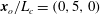
 $\boldsymbol{x}_{o}=(0,5L_{c},0)$
.
$\boldsymbol{x}_{o}=(0,5L_{c},0)$
.
2.4 Definition of variables for statistical analysis
Data processing and analysis are carried out upon the completion of each simulation. The main property required in this study is the power spectral density (PSD) function of the pressure fluctuations on the aerofoil surface and at the far-field observer location. The far-field (acoustic) pressure and the surface (wall) pressure jump are defined as:
 $$\begin{eqnarray}\displaystyle & \displaystyle p_{a}(\boldsymbol{x},t)=p(\boldsymbol{x},t)-p_{\infty }, & \displaystyle\end{eqnarray}$$
 $$\begin{eqnarray}\displaystyle & \displaystyle \unicode[STIX]{x0394}p_{w}(\boldsymbol{x},t)=\lim _{y\rightarrow 0^{+}}p(\boldsymbol{x},t)-\lim _{y\rightarrow 0^{-}}p(\boldsymbol{x},t), & \displaystyle\end{eqnarray}$$
where superscripts ‘
 $y\rightarrow 0^{+}$
’ and ‘
$y\rightarrow 0^{+}$
’ and ‘
 $y\rightarrow 0^{-}$
’ indicate the upper and lower surfaces of the zero-thickness aerofoil, respectively. Following the definitions used by Goldstein (Reference Goldstein1976), the PSD functions of the pressure fluctuations (based on frequency and one-sided) are then calculated as:
$y\rightarrow 0^{-}$
’ indicate the upper and lower surfaces of the zero-thickness aerofoil, respectively. Following the definitions used by Goldstein (Reference Goldstein1976), the PSD functions of the pressure fluctuations (based on frequency and one-sided) are then calculated as:
 $$\begin{eqnarray}\displaystyle & \displaystyle S_{ppa}(\boldsymbol{x},f)=\lim _{T\rightarrow \infty }\frac{P_{a}(\boldsymbol{x},f,T)P_{a}^{\ast }(\boldsymbol{x},f,T)}{T}, & \displaystyle\end{eqnarray}$$
 $$\begin{eqnarray}\displaystyle & \displaystyle S_{ppw}(\boldsymbol{x},f)=\lim _{T\rightarrow \infty }\frac{\unicode[STIX]{x0394}P_{w}(\boldsymbol{x},f,T)\unicode[STIX]{x0394}P_{w}^{\ast }(\boldsymbol{x},f,T)}{T}. & \displaystyle\end{eqnarray}$$
Here
 $P_{a}$
and
$P_{a}$
and
 $\unicode[STIX]{x0394}P_{w}$
are an approximate Fourier transform of
$\unicode[STIX]{x0394}P_{w}$
are an approximate Fourier transform of
 $p_{a}$
and
$p_{a}$
and
 $\unicode[STIX]{x0394}p_{w}$
, respectively, based on the following definition,
$\unicode[STIX]{x0394}p_{w}$
, respectively, based on the following definition,
 $$\begin{eqnarray}\displaystyle & \displaystyle P_{a}(\boldsymbol{x},f,T)=\int _{-T}^{T}p_{a}(\boldsymbol{x},t)\text{e}^{2\unicode[STIX]{x03C0}\text{i}ft}\,\text{d}t, & \displaystyle\end{eqnarray}$$
 $$\begin{eqnarray}\displaystyle & \displaystyle \unicode[STIX]{x0394}P_{w}(\boldsymbol{x},f,T)=\int _{-T}^{T}\unicode[STIX]{x0394}p_{w}(\boldsymbol{x},t)\text{e}^{2\unicode[STIX]{x03C0}\text{i}ft}\,\text{d}t. & \displaystyle\end{eqnarray}$$
In (2.10) and (2.11), ‘
 $\ast$
’ denotes a complex conjugate. The frequency-dependent noise reduction (NR) due to a WLE relative to the SLE case is then quantified by
$\ast$
’ denotes a complex conjugate. The frequency-dependent noise reduction (NR) due to a WLE relative to the SLE case is then quantified by
 $$\begin{eqnarray}\displaystyle \text{NR}(\boldsymbol{x},f)=\frac{S_{ppa}(\boldsymbol{x},f)|_{SLE}}{S_{ppa}(\boldsymbol{x},f)|_{WLE}}. & & \displaystyle\end{eqnarray}$$
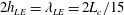
Also, we define a dimensionless frequency (Strouhal number) based on the peak-to-root amplitude of WLE (
 $2h_{LE}$
) and the free-stream velocity (
$2h_{LE}$
) and the free-stream velocity (
 $u_{\infty }$
), which is used for the majority of the current investigations, as
$u_{\infty }$
), which is used for the majority of the current investigations, as
 $$\begin{eqnarray}\displaystyle St_{LE}=\frac{2fh_{LE}}{u_{\infty }}. & & \displaystyle\end{eqnarray}$$
3 Universal trends and LE-focused one-dimensional analysis

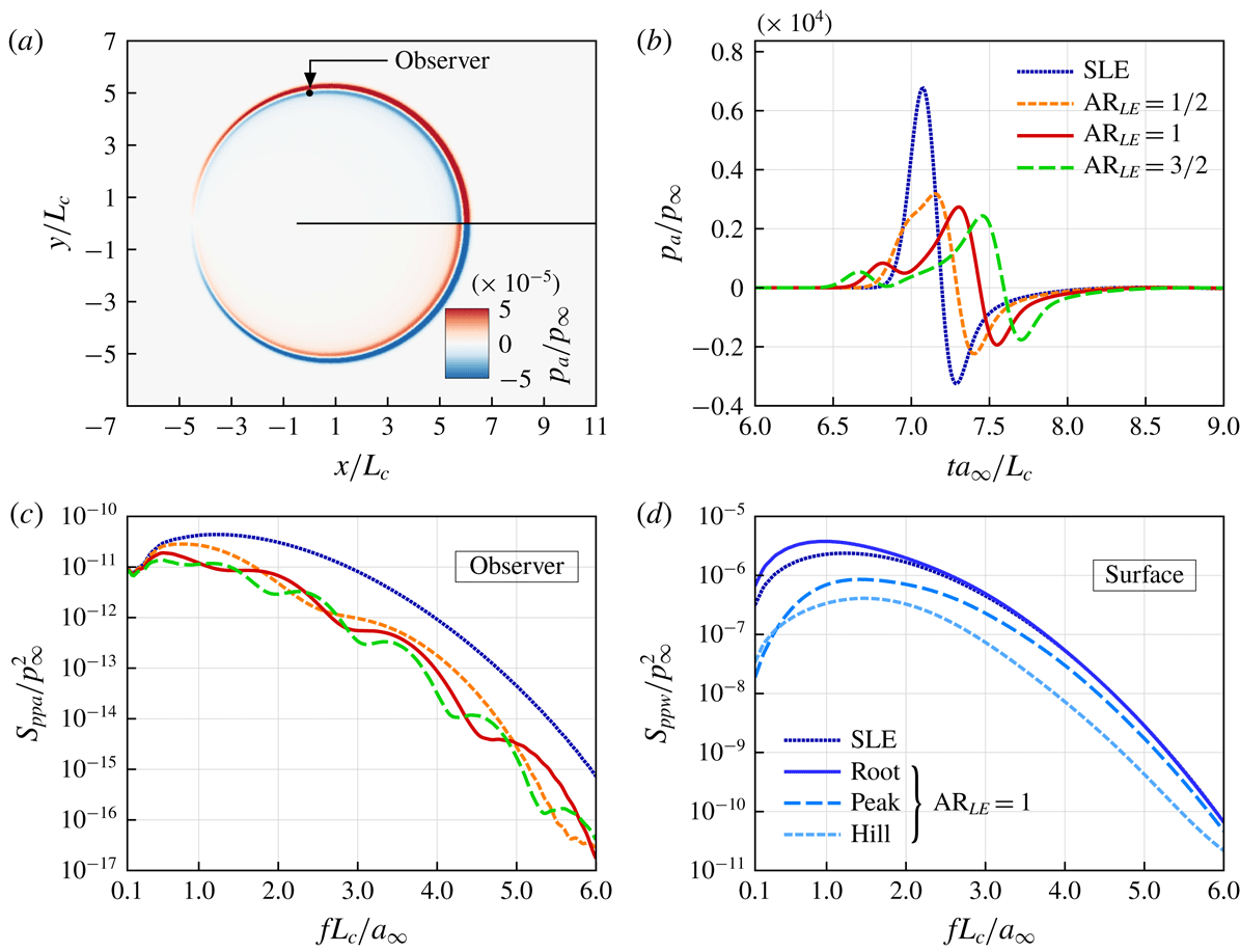
Figure 2. (a) An instantaneous contour plot of
 $p_{a}(\boldsymbol{x}_{o},ta_{\infty }/L_{c}=7.34)/p_{\infty }$
taken at mid-span (
$p_{a}(\boldsymbol{x}_{o},ta_{\infty }/L_{c}=7.34)/p_{\infty }$
taken at mid-span (
 $z=0$
) for the SLE case. (b) Time signals of acoustic pressure
$z=0$
) for the SLE case. (b) Time signals of acoustic pressure
 $p_{a}(\boldsymbol{x}_{o},t)/p_{\infty }$
obtained at an observer location
$p_{a}(\boldsymbol{x}_{o},t)/p_{\infty }$
obtained at an observer location
 $\boldsymbol{x}_{o}/L_{c}=(0,5,0)$
for SLE and three WLE geometries with differing aspect ratios (
$\boldsymbol{x}_{o}/L_{c}=(0,5,0)$
for SLE and three WLE geometries with differing aspect ratios (
 $\text{AR}_{LE}=2h_{LE}/\unicode[STIX]{x1D706}_{LE}$
). (c) The corresponding power spectra of the former. (d) The power spectra of wall pressure jump taken at the first grid cell aft of the LE, comparing SLE with WLE peak, hill and root, where the WLE aspect ratio is
$\text{AR}_{LE}=2h_{LE}/\unicode[STIX]{x1D706}_{LE}$
). (c) The corresponding power spectra of the former. (d) The power spectra of wall pressure jump taken at the first grid cell aft of the LE, comparing SLE with WLE peak, hill and root, where the WLE aspect ratio is
 $\text{AR}_{LE}=1$
.
$\text{AR}_{LE}=1$
.
Figure 2 shows some initial results of the current simulations comparing the SLE and WLE cases. In the figure, three different WLE aspect ratios are tested, i.e.
 $\text{AR}_{LE}=2h_{LE}/\unicode[STIX]{x1D706}_{LE}=1/2$
, 1 and
$\text{AR}_{LE}=2h_{LE}/\unicode[STIX]{x1D706}_{LE}=1/2$
, 1 and
 $3/2$
, where
$3/2$
, where
 $h_{LE}/L_{c}=1/30$
,
$h_{LE}/L_{c}=1/30$
,
 $1/15$
and
$1/15$
and
 $1/10$
(with
$1/10$
(with
 $\unicode[STIX]{x1D706}_{LE}/L_{c}=1/15$
fixed). An instantaneous snapshot of the radiating sound waves is captured in figure 2(a). The current result re-confirms the previous observations reported in the existing literature. The overall amplitude of the radiated sound pressure signal decreases when a larger WLE amplitude (
$\unicode[STIX]{x1D706}_{LE}/L_{c}=1/15$
fixed). An instantaneous snapshot of the radiating sound waves is captured in figure 2(a). The current result re-confirms the previous observations reported in the existing literature. The overall amplitude of the radiated sound pressure signal decreases when a larger WLE amplitude (
 $h_{LE}$
) is used (figure 2
b). The corresponding sound power spectra (figure 2
c) show that the difference between the SLE and WLE cases grows progressively with frequency whereas the difference vanishes at low frequencies. In the meantime, seemingly the reversed trends are observed in the source (wall pressure jump) power spectra obtained at some LE points (figure 2
d). The conflicting trends have also been reported in Turner & Kim (Reference Turner and Kim2017). It is shown later in this paper that the conflicting issues are resolved when the downstream sources are taken into account.
$h_{LE}$
) is used (figure 2
b). The corresponding sound power spectra (figure 2
c) show that the difference between the SLE and WLE cases grows progressively with frequency whereas the difference vanishes at low frequencies. In the meantime, seemingly the reversed trends are observed in the source (wall pressure jump) power spectra obtained at some LE points (figure 2
d). The conflicting trends have also been reported in Turner & Kim (Reference Turner and Kim2017). It is shown later in this paper that the conflicting issues are resolved when the downstream sources are taken into account.

Figure 3. (a) Noise-reduction spectra defined in (2.14) obtained at the observer position shown in figure 2(a), for three different WLE aspect ratios. (b) Re-plot of them by using a rescaled frequency (Strouhal number),
 $St_{LE}=2fh_{LE}/u_{\infty }$
, re-confirming the self-similarity trend reported by Chaitanya et al. (Reference Chaitanya, Joseph, Narayanan, Vanderwel, Turner, Kim and Ganapathisubramani2017):
$St_{LE}=2fh_{LE}/u_{\infty }$
, re-confirming the self-similarity trend reported by Chaitanya et al. (Reference Chaitanya, Joseph, Narayanan, Vanderwel, Turner, Kim and Ganapathisubramani2017):
 $\text{NR}=5St_{LE}$
.
$\text{NR}=5St_{LE}$
.
Figure 3 shows the relative NR (noise reduction) made by the WLEs as a function of frequency defined in (2.14). In particular, figure 3(b) reveals a self-similarity between the NR spectra which appears when the frequency is rescaled by using
 $2h_{LE}$
(peak-to-root distance) and
$2h_{LE}$
(peak-to-root distance) and
 $u_{\infty }$
(vortex convection speed) as suggested by Chaitanya et al. (Reference Chaitanya, Joseph, Narayanan, Vanderwel, Turner, Kim and Ganapathisubramani2017). As mentioned earlier in § 1, there are two universal trends in the NR spectra which have widely been observed in the previous literature. These are also captured in figure 3(b). Firstly, NR vanishes as the frequency approaches zero. Secondly, the level of NR grows consistently with frequency (apart from the oscillatory patterns), reaching 10 dB at about
$u_{\infty }$
(vortex convection speed) as suggested by Chaitanya et al. (Reference Chaitanya, Joseph, Narayanan, Vanderwel, Turner, Kim and Ganapathisubramani2017). As mentioned earlier in § 1, there are two universal trends in the NR spectra which have widely been observed in the previous literature. These are also captured in figure 3(b). Firstly, NR vanishes as the frequency approaches zero. Secondly, the level of NR grows consistently with frequency (apart from the oscillatory patterns), reaching 10 dB at about
 $St_{LE}\approx 1.5$
. However, accurate explanations as to how the universal trends are constructed have not been achieved although two possible scenarios were suggested by Chaitanya et al. (Reference Chaitanya, Joseph, Narayanan, Vanderwel, Turner, Kim and Ganapathisubramani2017). They demonstrated that a linearly growing trend of NR (i.e.
$St_{LE}\approx 1.5$
. However, accurate explanations as to how the universal trends are constructed have not been achieved although two possible scenarios were suggested by Chaitanya et al. (Reference Chaitanya, Joseph, Narayanan, Vanderwel, Turner, Kim and Ganapathisubramani2017). They demonstrated that a linearly growing trend of NR (i.e.
 $\text{NR}=5St_{LE}$
) could be obtained by considering either: (i) predicted phase variations of the source signal along the WLE but no change in the magnitude; or, (ii) no phase variation but the line-integrated source magnitude diminishing inversely with frequency (which is a hypothesis). Clarifications to these rather conflicting theories are provided later in this paper.
$\text{NR}=5St_{LE}$
) could be obtained by considering either: (i) predicted phase variations of the source signal along the WLE but no change in the magnitude; or, (ii) no phase variation but the line-integrated source magnitude diminishing inversely with frequency (which is a hypothesis). Clarifications to these rather conflicting theories are provided later in this paper.
It is worth noting that the oscillatory patterns in figure 3(b) may be linked with the source phase interference since the local maxima correspond to the case where the peak and the root emit sound waves
 $180^{\circ }$
out of phase (
$180^{\circ }$
out of phase (
 $St_{LE}=n\pm 1/2$
where
$St_{LE}=n\pm 1/2$
where
 $n$
is an integer) and the local minima correspond to the opposite case emitting in phase (
$n$
is an integer) and the local minima correspond to the opposite case emitting in phase (
 $St_{LE}=n$
), in other words
$St_{LE}=n$
), in other words
 $$\begin{eqnarray}\displaystyle 2\unicode[STIX]{x03C0}St_{LE}=\left\{\begin{array}{@{}l@{}}(2n\pm 1)\unicode[STIX]{x03C0}:180^{\circ }\text{ out of phase (destructive interference),}\\ 2n\unicode[STIX]{x03C0}:\text{in phase (constructive interference).}\end{array}\right. & & \displaystyle\end{eqnarray}$$
This phase relationship indicates that increasing
 $h_{LE}$
forces the destructive interference to appear at a lower frequency as shown in figure 3(a) (for
$h_{LE}$
forces the destructive interference to appear at a lower frequency as shown in figure 3(a) (for
 $fL_{c}/a_{\infty }<1$
). Therefore, the overall NR based on overall sound pressure level grows with
$fL_{c}/a_{\infty }<1$
). Therefore, the overall NR based on overall sound pressure level grows with
 $h_{LE}$
since most of the acoustic energy is contained in the low frequency range. Another observation to make in figure 3(b) is that the local maxima in the spectra decrease with increasing
$h_{LE}$
since most of the acoustic energy is contained in the low frequency range. Another observation to make in figure 3(b) is that the local maxima in the spectra decrease with increasing
 $h_{LE}$
. It is attributed to the fact that the peak and the root have different source magnitude (as shown in figure 2
d) and the difference becomes larger as
$h_{LE}$
. It is attributed to the fact that the peak and the root have different source magnitude (as shown in figure 2
d) and the difference becomes larger as
 $h_{LE}$
increases (Kim et al.
Reference Kim, Haeri and Joseph2016; Turner & Kim Reference Turner and Kim2017). The unequal source magnitude between the peak and the root means that their destructive interference becomes less efficient at the frequencies of
$h_{LE}$
increases (Kim et al.
Reference Kim, Haeri and Joseph2016; Turner & Kim Reference Turner and Kim2017). The unequal source magnitude between the peak and the root means that their destructive interference becomes less efficient at the frequencies of
 $St_{LE}=n\pm 1/2$
. Therefore the non-uniformity of source magnitude as well as the phase interference plays an important role in the NR spectra.
$St_{LE}=n\pm 1/2$
. Therefore the non-uniformity of source magnitude as well as the phase interference plays an important role in the NR spectra.
Having critically reviewed the latest progress made in the study of WLEs, however, we still have not reached conclusive answers to the two fundamental questions raised earlier: (i) why NR vanishes at low frequencies; and, (ii) what drives the consistent growth of NR at high frequencies. On a level below, what are the balances between the non-uniform distribution of the source magnitude and the constructive/destructive phase interference that we need to understand in order to answer the questions? There is a lack of information/data made available to properly answer these questions. It should be noted here that all of the previous studies are focused only on the LE source distribution neglecting the downstream sources (assuming the dominance of the LE source irrespective of frequency), which is a one-dimensional (1-D) approach. The authors have found that the LE-focused 1-D approach fails to deliver sufficient information and data that are necessary to answer the questions.
4 The significance of two-dimensional source distribution
In this section, the LE-focused 1-D source assumption is discarded and the investigation is expanded into two dimensions across the entire aerofoil surface to include the downstream sources that have been neglected in the past. It is discovered in this section that the source distribution becomes significantly two-dimensional (2-D) (highly non-uniform in the spanwise direction as well as streamwise) in the WLE case. It is also found that the downstream sources are far from negligible at high frequencies for both SLE and WLE. These new observations are leading to profound conclusions at the end of the paper.
4.1 Acoustic source map varying with frequency

Figure 4. Contour plots of the level of wall pressure jump (source magnitude) represented by
 $|\unicode[STIX]{x0394}P_{w}(x,z,f)|/p_{ref}$
in a logarithmic scale (
$|\unicode[STIX]{x0394}P_{w}(x,z,f)|/p_{ref}$
in a logarithmic scale (
 $p_{ref}=10^{-10}p_{\infty }$
), at two different frequencies (in the low range):
$p_{ref}=10^{-10}p_{\infty }$
), at two different frequencies (in the low range):
 $St_{LE}=0.1$
and 0.5, for the SLE and WLE cases, respectively. The length scales used are
$St_{LE}=0.1$
and 0.5, for the SLE and WLE cases, respectively. The length scales used are
 $2h_{LE}=\unicode[STIX]{x1D706}_{LE}=2L_{c}/15$
(
$2h_{LE}=\unicode[STIX]{x1D706}_{LE}=2L_{c}/15$
(
 $\text{AR}_{LE}=1$
). As indicated earlier,
$\text{AR}_{LE}=1$
). As indicated earlier,
 $\unicode[STIX]{x0394}P_{w}(\boldsymbol{x},f)$
is the Fourier transform of the wall pressure jump
$\unicode[STIX]{x0394}P_{w}(\boldsymbol{x},f)$
is the Fourier transform of the wall pressure jump
 $\unicode[STIX]{x0394}p_{w}(\boldsymbol{x},t)$
.
$\unicode[STIX]{x0394}p_{w}(\boldsymbol{x},t)$
.

Figure 5. Contour plots of the level of wall pressure jump (source magnitude) represented by
 $|\unicode[STIX]{x0394}P_{w}(x,z,f)|/p_{ref}$
in a logarithmic scale (
$|\unicode[STIX]{x0394}P_{w}(x,z,f)|/p_{ref}$
in a logarithmic scale (
 $p_{ref}=10^{-10}p_{\infty }$
), at four different frequencies (in the high range):
$p_{ref}=10^{-10}p_{\infty }$
), at four different frequencies (in the high range):
 $St_{LE}=2$
, 2.5, 3 and 3.5, for the SLE and WLE cases, respectively. As indicated earlier,
$St_{LE}=2$
, 2.5, 3 and 3.5, for the SLE and WLE cases, respectively. As indicated earlier,
 $\unicode[STIX]{x0394}P_{w}(\boldsymbol{x},f)$
is the Fourier transform of the wall pressure jump
$\unicode[STIX]{x0394}P_{w}(\boldsymbol{x},f)$
is the Fourier transform of the wall pressure jump
 $\unicode[STIX]{x0394}p_{w}(\boldsymbol{x},t)$
.
$\unicode[STIX]{x0394}p_{w}(\boldsymbol{x},t)$
.
Two-dimensional distributions of the noise source (wall pressure jump) magnitude on the aerofoil surface, represented by
 $|\unicode[STIX]{x0394}P_{w}(x,y=0,z,f)|$
, are plotted in figures 4 and 5 for various frequencies. At the low frequencies (figure 4) it is obvious that the source distribution is highly concentrated at the leading edge in both the SLE and WLE cases. Also, the distribution pattern (despite the level change) seems to remain almost unchanged in the low frequency range, although the WLE case exhibits a moderate change (growth) in the peak area as the frequency increases from
$|\unicode[STIX]{x0394}P_{w}(x,y=0,z,f)|$
, are plotted in figures 4 and 5 for various frequencies. At the low frequencies (figure 4) it is obvious that the source distribution is highly concentrated at the leading edge in both the SLE and WLE cases. Also, the distribution pattern (despite the level change) seems to remain almost unchanged in the low frequency range, although the WLE case exhibits a moderate change (growth) in the peak area as the frequency increases from
 $St_{LE}=0.1$
to 0.5. This suggests that the LE-focused 1-D source assumption is valid at least in the low frequency range. However, it is shown in figure 5 that the 1-D assumption is no longer valid at high frequencies. Firstly, in both the SLE and WLE cases, the source magnitude downstream of the LE increases significantly with frequency, and eventually it becomes comparable to that of the LE (within certain areas of the surface) at
$St_{LE}=0.1$
to 0.5. This suggests that the LE-focused 1-D source assumption is valid at least in the low frequency range. However, it is shown in figure 5 that the 1-D assumption is no longer valid at high frequencies. Firstly, in both the SLE and WLE cases, the source magnitude downstream of the LE increases significantly with frequency, and eventually it becomes comparable to that of the LE (within certain areas of the surface) at
 $St_{LE}>3$
as shown in figure 5(c,d). Secondly, the source distribution pattern becomes entirely two-dimensional (highly non-uniform in the spanwise direction as well as streamwise) in the WLE case.
$St_{LE}>3$
as shown in figure 5(c,d). Secondly, the source distribution pattern becomes entirely two-dimensional (highly non-uniform in the spanwise direction as well as streamwise) in the WLE case.

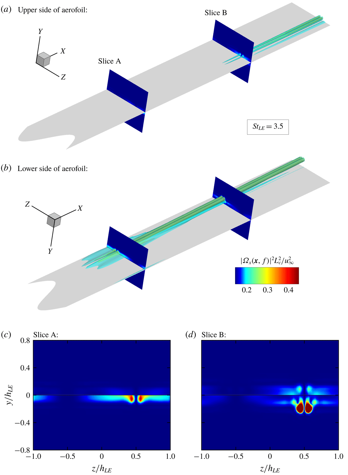
Figure 6. Iso-surfaces and contour plots of streamwise vorticity magnitude squared at the frequency of
 $St_{LE}=3.5$
, obtained via a Fourier transform of the vorticity time signals. The footprints of the strong streamwise vorticity downstream of the root correspond to the narrow strip of intensified source shown in figure 5(c,d).
$St_{LE}=3.5$
, obtained via a Fourier transform of the vorticity time signals. The footprints of the strong streamwise vorticity downstream of the root correspond to the narrow strip of intensified source shown in figure 5(c,d).
A unique feature appearing in the WLE case is that a narrow streamwise strip of strong source area is created downstream of the root at the high frequencies (figure 5
c,d). The authors suggest that it is mainly due to secondary vortical structures induced as part of the three-dimensional vortex dynamics taking place after the impinging vortex being bisected at the LE. In order to visualise this, a Fourier transform of the streamwise vorticity,
 $\unicode[STIX]{x1D6FA}_{x}(\boldsymbol{x},f)$
is calculated in the entire domain. Figure 6 shows the iso-surfaces and cross-sectional contour plots of
$\unicode[STIX]{x1D6FA}_{x}(\boldsymbol{x},f)$
is calculated in the entire domain. Figure 6 shows the iso-surfaces and cross-sectional contour plots of
 $|\unicode[STIX]{x1D6FA}_{x}(\boldsymbol{x},f)|^{2}$
at
$|\unicode[STIX]{x1D6FA}_{x}(\boldsymbol{x},f)|^{2}$
at
 $St_{LE}=3.5$
for the upper and lower parts of the aerofoil, respectively. The figure shows a clear footprint of streamwise vortices downstream of the root at the high frequency. More importantly, the streamwise vortices are stronger on the lower side of the aerofoil than that on the upper, and this asymmetry results in a pressure jump across the surface creating the narrow strip of strong source area.
$St_{LE}=3.5$
for the upper and lower parts of the aerofoil, respectively. The figure shows a clear footprint of streamwise vortices downstream of the root at the high frequency. More importantly, the streamwise vortices are stronger on the lower side of the aerofoil than that on the upper, and this asymmetry results in a pressure jump across the surface creating the narrow strip of strong source area.
In the meantime, it is worth noting that the frequency-dependent source map shown in figure 5 reveals that the source magnitude along the WLE frontline remains fairly uniform, i.e. insignificant differences between the peak, hill and root areas, for all frequencies. This outcome is in fact contradictory to one of the hypotheses made by Chaitanya et al. (Reference Chaitanya, Joseph, Narayanan, Vanderwel, Turner, Kim and Ganapathisubramani2017). They previously anticipated that the source distribution would be highly localised around the root and the effective area/length of the localised source should decrease inversely with increasing frequency to account for the growth of NR (noise reduction). However, the current simulation result indicates otherwise and therefore it is suggested again that a full 2-D source distribution should be investigated in order to properly address the NR at high frequencies.
4.2 The characteristics of downstream sources

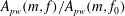
Figure 7. Normalised distributions of piecewise-integrated acoustic source magnitude,
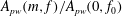 $A_{pw}(m,f)/A_{pw}(0,f_{0})$
defined in (4.1), where
$A_{pw}(m,f)/A_{pw}(0,f_{0})$
defined in (4.1), where
 $f_{0}$
is the lowest frequency considered here, i.e.
$f_{0}$
is the lowest frequency considered here, i.e.
 $2f_{0}h_{LE}/u_{\infty }=0.1$
. The figure highlights the elevated level of source magnitude downstream of the LE at high frequencies, comparing the SLE and WLE cases.
$2f_{0}h_{LE}/u_{\infty }=0.1$
. The figure highlights the elevated level of source magnitude downstream of the LE at high frequencies, comparing the SLE and WLE cases.
Based on the source distribution maps obtained above, the contribution of the downstream sources can be estimated from various streamwise locations. The estimation is made by using the following definition:
 $$\begin{eqnarray}\displaystyle A_{pw}(m,f)=\int _{-(1/2)\unicode[STIX]{x1D706}_{LE}}^{(1/2)\unicode[STIX]{x1D706}_{LE}}\int _{x_{LE}(z)+m\unicode[STIX]{x0394}x}^{x_{LE}(z)+(m+1)\unicode[STIX]{x0394}x}|\unicode[STIX]{x0394}P_{w}(x,z,f)|\,\text{d}x\,\text{d}z, & & \displaystyle\end{eqnarray}$$
which is a piecewise surface integration of the source magnitude within a small segment area of
 $x_{LE}+m\unicode[STIX]{x0394}x\leqslant x\leqslant x_{LE}+(m+1)\unicode[STIX]{x0394}x$
(where
$x_{LE}+m\unicode[STIX]{x0394}x\leqslant x\leqslant x_{LE}+(m+1)\unicode[STIX]{x0394}x$
(where
 $m$
is a positive integer indicating the
$m$
is a positive integer indicating the
 $m$
th segment). For convenience, we use
$m$
th segment). For convenience, we use
 $\unicode[STIX]{x0394}x=h_{LE}$
where
$\unicode[STIX]{x0394}x=h_{LE}$
where
 $h_{LE}=\unicode[STIX]{x1D706}_{LE}/2=L_{c}/15$
. Figure 7 shows the calculated values of
$h_{LE}=\unicode[STIX]{x1D706}_{LE}/2=L_{c}/15$
. Figure 7 shows the calculated values of
 $A_{pw}(m,f)$
as a function of
$A_{pw}(m,f)$
as a function of
 $m$
for various values of
$m$
for various values of
 $f$
, comparing the SLE and WLE cases. The curves are normalised by the value from the LE segment (
$f$
, comparing the SLE and WLE cases. The curves are normalised by the value from the LE segment (
 $m=0$
) at the lowest frequency selected (
$m=0$
) at the lowest frequency selected (
 $2f_{0}h_{LE}/u_{\infty }=0.1$
). It is clear from the figure that, at the low-to-medium frequencies (
$2f_{0}h_{LE}/u_{\infty }=0.1$
). It is clear from the figure that, at the low-to-medium frequencies (
 $0.1<St_{LE}<2.5$
), the source magnitude decays exponentially and continuously as the distance from the LE increases, in both the SLE and WLE cases. The curves also show a good level of self-similarity between them in the low-to-medium frequency range although the WLE case displays some more variations than the SLE case. However, at the high frequencies (
$0.1<St_{LE}<2.5$
), the source magnitude decays exponentially and continuously as the distance from the LE increases, in both the SLE and WLE cases. The curves also show a good level of self-similarity between them in the low-to-medium frequency range although the WLE case displays some more variations than the SLE case. However, at the high frequencies (
 $St_{LE}>2.5$
), the self-similarity breaks down and a significantly elevated level of source magnitude appears downstream of the LE, as hinted earlier in figure 5(c,d). The elevated high-frequency sources cover a large area and therefore their contribution to the far-field noise is expected to be significant for those frequencies. In addition, a striking feature found in figure 7 is that the source magnitude at the LE area is no longer the greatest when the frequency reaches
$St_{LE}>2.5$
), the self-similarity breaks down and a significantly elevated level of source magnitude appears downstream of the LE, as hinted earlier in figure 5(c,d). The elevated high-frequency sources cover a large area and therefore their contribution to the far-field noise is expected to be significant for those frequencies. In addition, a striking feature found in figure 7 is that the source magnitude at the LE area is no longer the greatest when the frequency reaches
 $St_{LE}=3.5$
in both the SLE and WLE cases. This is a compelling evidence that the LE-focused 1-D source assumption is invalid at high frequencies. The precision of the current result at the high frequencies has been double checked via a grid refinement test as shown in figure 8.
$St_{LE}=3.5$
in both the SLE and WLE cases. This is a compelling evidence that the LE-focused 1-D source assumption is invalid at high frequencies. The precision of the current result at the high frequencies has been double checked via a grid refinement test as shown in figure 8.

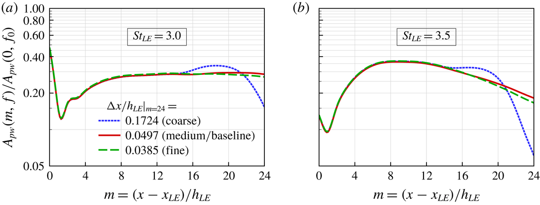
Figure 8. Validation of the grid resolution used in the current simulations, in order to ensure that a sufficient level of precision is presented in figure 7 at the highest frequencies (
 $St_{LE}=3.0$
and 3.5). Three different levels of grid resolution are tested for the WLE case, where the baseline and refined grids produce consistent results.
$St_{LE}=3.0$
and 3.5). Three different levels of grid resolution are tested for the WLE case, where the baseline and refined grids produce consistent results.

Figure 9. Normalised profiles of acoustic source magnitude as a function of frequency, integrated over each segment area described in (4.1),
 $A_{pw}(m,f)/A_{pw}(m,f_{0})$
where
$A_{pw}(m,f)/A_{pw}(m,f_{0})$
where
 $2f_{0}h_{LE}/u_{\infty }=0.1$
and
$2f_{0}h_{LE}/u_{\infty }=0.1$
and
 $m=(x-x_{LE})/h_{LE}$
. The figure re-confirms the trend of elevated source magnitude downstream of the LE at high frequencies shown in figure 7.
$m=(x-x_{LE})/h_{LE}$
. The figure re-confirms the trend of elevated source magnitude downstream of the LE at high frequencies shown in figure 7.
Having identified the significant variation of source magnitude downstream of the LE at high frequencies, particularly pronounced in the WLE case, it is worth checking the details of the frequency contents of the source contained within each segment area – defined in (4.1) – in order to see how they change as the distance from the LE increases. Figure 9 shows
 $A_{pw}(m,f)/A_{pw}(m,f_{0})$
(normalised by the values at the lowest frequency,
$A_{pw}(m,f)/A_{pw}(m,f_{0})$
(normalised by the values at the lowest frequency,
 $f_{0}$
, i.e.
$f_{0}$
, i.e.
 $2f_{0}h_{LE}/u_{\infty }=0.1$
) as a function of
$2f_{0}h_{LE}/u_{\infty }=0.1$
) as a function of
 $f$
for various values of
$f$
for various values of
 $m$
, comparing the SLE and WLE cases. In this figure, it is worth noting that the normalisation changes with
$m$
, comparing the SLE and WLE cases. In this figure, it is worth noting that the normalisation changes with
 $m$
, which is different from the normalisation used in the previous figure. The current figure reveals a few interesting outcomes. Firstly, there is a high level of self-similarity between the normalised frequency spectra (up to certain frequencies) in both the SLE and WLE cases. The self-similarity is particularly strong in the SLE case, hence almost irrespective of the downstream location of the source segment before diverging at the high frequencies. Secondly, in the WLE case, the self-similarity appears only amongst the downstream sources (
$m$
, which is different from the normalisation used in the previous figure. The current figure reveals a few interesting outcomes. Firstly, there is a high level of self-similarity between the normalised frequency spectra (up to certain frequencies) in both the SLE and WLE cases. The self-similarity is particularly strong in the SLE case, hence almost irrespective of the downstream location of the source segment before diverging at the high frequencies. Secondly, in the WLE case, the self-similarity appears only amongst the downstream sources (
 $m\geqslant 1$
), whereas the source right at the LE (
$m\geqslant 1$
), whereas the source right at the LE (
 $m=0$
) behaves very differently. The WLE source at
$m=0$
) behaves very differently. The WLE source at
 $m=0$
turns out very similar to the SLE sources. The distinctive difference between the LE and downstream sources in the WLE case is another evidence that the LE-focused 1-D analysis fails to work for WLE noise prediction. Thirdly, there exists an elevated level of source magnitude appearing at high frequencies downstream of the LE, commonly in both the SLE and WLE cases, indicating again the significance of the downstream source contribution.
$m=0$
turns out very similar to the SLE sources. The distinctive difference between the LE and downstream sources in the WLE case is another evidence that the LE-focused 1-D analysis fails to work for WLE noise prediction. Thirdly, there exists an elevated level of source magnitude appearing at high frequencies downstream of the LE, commonly in both the SLE and WLE cases, indicating again the significance of the downstream source contribution.
5 Towards understanding the universal trends
The next step of the investigation is to quantify the contribution of the downstream sources in terms of the estimated sound pressure level (SPL) and to compare the SLE and WLE cases. For this purpose, we consider a quantity defined by
 $$\begin{eqnarray}\displaystyle B_{pw}(m,f)=\left[\mathop{\sum }_{j=0}^{m}A_{pw}(j,f)\right]^{2}, & & \displaystyle\end{eqnarray}$$
which is a representative estimation of SPL at the source based on a surface integral that runs from the LE to a given downstream location
 $x=x_{LE}+(m+1)h_{LE}$
(up to the
$x=x_{LE}+(m+1)h_{LE}$
(up to the
 $m$
th segment area). It is purely based on the magnitude of the source with no phase variation included. The ratio of
$m$
th segment area). It is purely based on the magnitude of the source with no phase variation included. The ratio of
 $B_{pw}(m,f)$
between the SLE and WLE cases represent the level of source reduction (SR) based on the magnitude, defined as
$B_{pw}(m,f)$
between the SLE and WLE cases represent the level of source reduction (SR) based on the magnitude, defined as
 $$\begin{eqnarray}\displaystyle \text{SR}_{mag}(m,f)=\frac{B_{pw}(m,f)|_{SLE}}{B_{pw}(m,f)|_{WLE}}, & & \displaystyle\end{eqnarray}$$
which can be compared to the far-field noise reduction (NR) defined in (2.14).
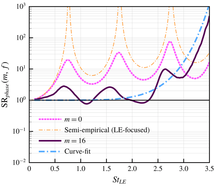
5.1 Invariant source magnitude at low frequencies
Figure 10 shows the magnitude-based SR (source reduction) spectrum for various values of
 $m$
. In figure 10(a), it is shown that the SR spectrum changes significantly due to the downstream contributions. As more downstream sources are included, SR increases in the medium frequency range whereas the opposite takes place in the low and high frequency ranges. The SR spectrum including the downstream contribution (
$m$
. In figure 10(a), it is shown that the SR spectrum changes significantly due to the downstream contributions. As more downstream sources are included, SR increases in the medium frequency range whereas the opposite takes place in the low and high frequency ranges. The SR spectrum including the downstream contribution (
 $m=16$
), compared to the LE-focused case (
$m=16$
), compared to the LE-focused case (
 $m=0$
), agrees very well with the far-field NR (noise reduction) spectrum for frequencies up to approximately
$m=0$
), agrees very well with the far-field NR (noise reduction) spectrum for frequencies up to approximately
 $St_{LE}\approx 2.5$
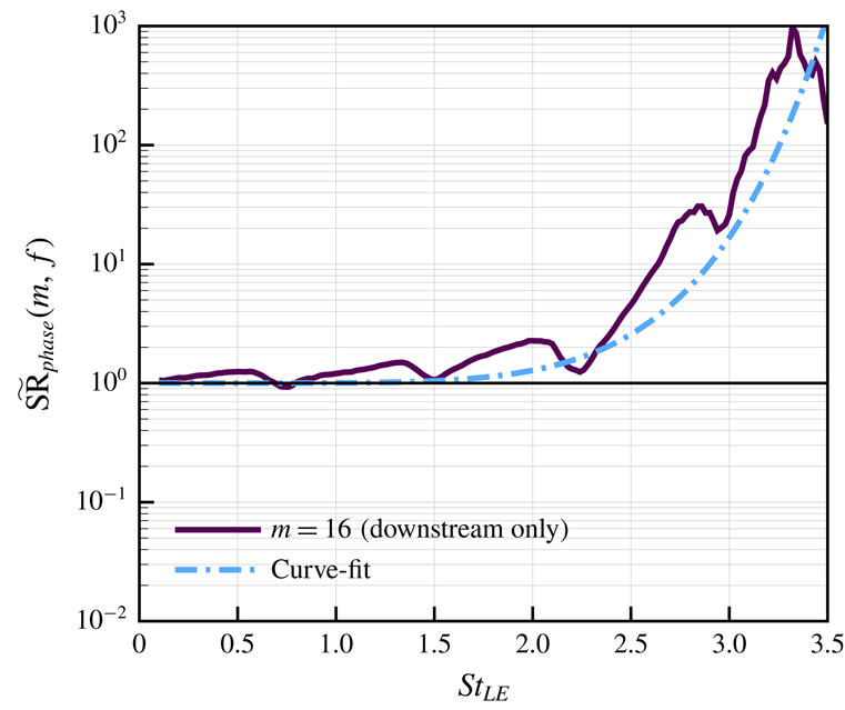
, as shown in figure 10(b). However, there is a sudden decay of SR at the higher frequencies, which is due to the elevated level of the downstream sources in the WLE case as observed in § 4. This means that the SR spectrum purely based on the magnitude fails to deliver a reasonable estimation of NR at the high frequencies. It is crucial to include phase variations in the SR spectrum in order to properly account for the high frequency range (to follow later in this section).
$St_{LE}\approx 2.5$
, as shown in figure 10(b). However, there is a sudden decay of SR at the higher frequencies, which is due to the elevated level of the downstream sources in the WLE case as observed in § 4. This means that the SR spectrum purely based on the magnitude fails to deliver a reasonable estimation of NR at the high frequencies. It is crucial to include phase variations in the SR spectrum in order to properly account for the high frequency range (to follow later in this section).

Figure 10. Magnitude-based SR (source reduction) spectra,
 $\text{SR}_{mag}(m,f)$
defined in (5.2), plotted for various values of
$\text{SR}_{mag}(m,f)$
defined in (5.2), plotted for various values of
 $m$
. The SR spectra are compared with the far-field NR (noise reduction) spectrum on the right.
$m$
. The SR spectra are compared with the far-field NR (noise reduction) spectrum on the right.
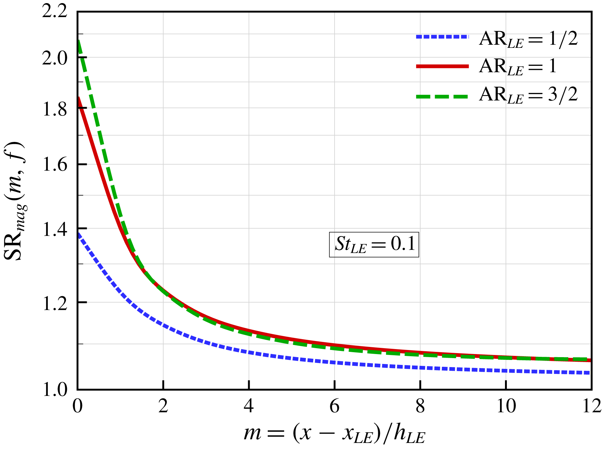
Figure 11. The convergence of source reduction,
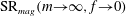 $\text{SR}_{mag}(m\rightarrow \infty ,f\rightarrow 0)$
 $\rightarrow 1.0$
, calculated at a low frequency (
$\rightarrow 1.0$
, calculated at a low frequency (
 $St_{LE}=0.1$
) for three different WLE profiles used. This figure suggests that the total source energy (integrated over a large surface area) at a low frequency remains unchanged irrespective of the LE geometry. This explains the universal trend of NR vanishing at low frequencies.
$St_{LE}=0.1$
) for three different WLE profiles used. This figure suggests that the total source energy (integrated over a large surface area) at a low frequency remains unchanged irrespective of the LE geometry. This explains the universal trend of NR vanishing at low frequencies.
In figure 10(b), it is remarkable that the SR spectrum with the downstream contributions included (
 $m=16$
) accurately reproduces the universal trend of NR vanishing at low frequencies. On the other hand, the LE-focused result (
$m=16$
) accurately reproduces the universal trend of NR vanishing at low frequencies. On the other hand, the LE-focused result (
 $m=0$
) falsely predicts a significant level of NR. More details of the low-frequency events are provided in figure 11. It is revealed in the figure that the value of SR converges to unity at a low frequency as more downstream sources are included, i.e.
$m=0$
) falsely predicts a significant level of NR. More details of the low-frequency events are provided in figure 11. It is revealed in the figure that the value of SR converges to unity at a low frequency as more downstream sources are included, i.e.
 $\text{SR}_{mag}(m\rightarrow \infty ,f\rightarrow 0)\rightarrow 1.0$
. This is consistently true for three different WLE profiles used. This outcome suggests that, at low frequencies, the total amount of source energy integrated over the entire surface remains preserved regardless of geometric changes at the LE. This forms a reasonable explanation to the universal trend of NR vanishing at low frequencies which has widely been observed to date.
$\text{SR}_{mag}(m\rightarrow \infty ,f\rightarrow 0)\rightarrow 1.0$
. This is consistently true for three different WLE profiles used. This outcome suggests that, at low frequencies, the total amount of source energy integrated over the entire surface remains preserved regardless of geometric changes at the LE. This forms a reasonable explanation to the universal trend of NR vanishing at low frequencies which has widely been observed to date.
5.2 Inclusion of phase variations

Figure 12. Magnitude-and-phase-based SR (source reduction) spectra,
 $\text{SR}_{mag\& phase}(m,f)$
defined in (5.5), plotted for various values of
$\text{SR}_{mag\& phase}(m,f)$
defined in (5.5), plotted for various values of
 $m$
. The SR spectra are compared with the far-field NR (noise reduction) spectrum on the right.
$m$
. The SR spectra are compared with the far-field NR (noise reduction) spectrum on the right.
In the meantime, the second universal trend of NR growing consistently with frequency (in the medium-to-high frequency range) is not captured in the magnitude-based SR spectrum. As hinted earlier, the source phase interference is of significant importance in order to address the high frequency range and therefore the following quantities are defined (similarly to those used earlier) in order to include the phase variations in the investigation,
 $$\begin{eqnarray}\displaystyle & \displaystyle C_{pw}(m,f)=\int _{-(1/2)\unicode[STIX]{x1D706}_{LE}}^{(1/2)\unicode[STIX]{x1D706}_{LE}}\int _{x_{LE}(z)+m\unicode[STIX]{x0394}x}^{x_{LE}(z)+(m+1)\unicode[STIX]{x0394}x}\unicode[STIX]{x0394}P_{w}(x,z,f)\,\text{d}x\,\text{d}z, & \displaystyle\end{eqnarray}$$
 $$\begin{eqnarray}\displaystyle & \displaystyle D_{pw}(m,f)=\left|\mathop{\sum }_{j=0}^{m}C_{pw}(j,f)\right|^{2}. & \displaystyle\end{eqnarray}$$
These are similar to
 $A_{pw}(m,f)$
and
$A_{pw}(m,f)$
and
 $B_{pw}(m,f)$
in (4.1) and (5.1), respectively, except that the real and imaginary parts of
$B_{pw}(m,f)$
in (4.1) and (5.1), respectively, except that the real and imaginary parts of
 $\unicode[STIX]{x0394}P_{w}(x,z,f)$
are maintained separately in the formula until the final value of
$\unicode[STIX]{x0394}P_{w}(x,z,f)$
are maintained separately in the formula until the final value of
 $D_{pw}(m,f)$
is determined. This allows for the phase interference taking place during the surface integration. This approach is actually equivalent to the Ffowcs Williams–Hawkings (FW-H) integration of sources (Ffowcs Williams & Hawkings Reference Ffowcs Williams and Hawkings1969) without considering an observer’s retarded time. Based on this approach, a new SR spectrum based on the magnitude and phase combined can be defined as
$D_{pw}(m,f)$
is determined. This allows for the phase interference taking place during the surface integration. This approach is actually equivalent to the Ffowcs Williams–Hawkings (FW-H) integration of sources (Ffowcs Williams & Hawkings Reference Ffowcs Williams and Hawkings1969) without considering an observer’s retarded time. Based on this approach, a new SR spectrum based on the magnitude and phase combined can be defined as
 $$\begin{eqnarray}\displaystyle \text{SR}_{mag\& phase}(m,f)=\frac{D_{pw}(m,f)|_{SLE}}{D_{pw}(m,f)|_{WLE}}. & & \displaystyle\end{eqnarray}$$
The magnitude-and-phase-based SR spectra are plotted in figure 12 for various values of
 $m$
. It is noticeable that the inclusion of the phase variations, compared to the magnitude-only case, gives rise to the oscillatory patterns in the spectra and also to the level of SR at the high frequencies. This result indicates that the high frequency range is substantially contributed by the source phase interference whereas the low frequency range is mainly governed by the source magnitude attenuation. In figure 12(a), it is demonstrated again that the inclusion of the downstream sources makes significant changes in estimating the level of SR. Figure 12(b) shows that the SR spectrum based on both the magnitude and the phase obtained from a sufficiently large area (
$m$
. It is noticeable that the inclusion of the phase variations, compared to the magnitude-only case, gives rise to the oscillatory patterns in the spectra and also to the level of SR at the high frequencies. This result indicates that the high frequency range is substantially contributed by the source phase interference whereas the low frequency range is mainly governed by the source magnitude attenuation. In figure 12(a), it is demonstrated again that the inclusion of the downstream sources makes significant changes in estimating the level of SR. Figure 12(b) shows that the SR spectrum based on both the magnitude and the phase obtained from a sufficiently large area (
 $m=16$
) almost accurately reproduces the far-field NR spectrum in the entire frequency range. However, the LE-focused estimation (
$m=16$
) almost accurately reproduces the far-field NR spectrum in the entire frequency range. However, the LE-focused estimation (
 $m=0$
) results in a large over-prediction of NR (by up to a 10 dB) across all frequencies with the local maxima and minima shifted to higher frequencies.
$m=0$
) results in a large over-prediction of NR (by up to a 10 dB) across all frequencies with the local maxima and minima shifted to higher frequencies.
5.3 Dominance of source phase interference at high frequencies

Figure 13. Estimated contribution of phase interference to SR (source reduction) spectra,
 $\text{SR}_{phase}(m,f)$
defined in (5.6), comparing the LE-focused (
$\text{SR}_{phase}(m,f)$
defined in (5.6), comparing the LE-focused (
 $m=0$
) and surface-integrated (
$m=0$
) and surface-integrated (
 $m=16$
) cases. The LE-focused semi-empirical model
$m=16$
) cases. The LE-focused semi-empirical model
 $\text{NR}=J_{0}^{-2}(\unicode[STIX]{x03C0}St_{LE})$
was proposed by Chaitanya et al. (Reference Chaitanya, Joseph, Narayanan, Vanderwel, Turner, Kim and Ganapathisubramani2017). This figure indicates that the surface-integrated source phase interference is insignificant at low-to-medium frequencies but increases rapidly at high frequencies contributed by the downstream sources.
$\text{NR}=J_{0}^{-2}(\unicode[STIX]{x03C0}St_{LE})$
was proposed by Chaitanya et al. (Reference Chaitanya, Joseph, Narayanan, Vanderwel, Turner, Kim and Ganapathisubramani2017). This figure indicates that the surface-integrated source phase interference is insignificant at low-to-medium frequencies but increases rapidly at high frequencies contributed by the downstream sources.
It is now possible to estimate the contribution of the source phase variation/interference to NR based on
 $\text{SR}_{mag\& phase}(m,f)$
and
$\text{SR}_{mag\& phase}(m,f)$
and
 $\text{SR}_{mag}(m,f)$
that are obtained above. Although the phase interference is strongly coupled with the source magnitude distribution, the following may be defined to indirectly estimate the contribution of the phase interference,
$\text{SR}_{mag}(m,f)$
that are obtained above. Although the phase interference is strongly coupled with the source magnitude distribution, the following may be defined to indirectly estimate the contribution of the phase interference,
 $$\begin{eqnarray}\displaystyle \text{SR}_{phase}(m,f)=\frac{\text{SR}_{mag\& phase}(m,f)}{\text{SR}_{mag}(m,f)}. & & \displaystyle\end{eqnarray}$$
Figure 13 shows the above defined phase-based SR spectrum comparing the LE-focused (
 $m=0$
) and surface-integrated (
$m=0$
) and surface-integrated (
 $m=16$
) cases. Firstly, it is indicated in the surface-integrated case that the level of source phase interference (contributing to NR) is insignificant in the low-to-medium frequency range although there are oscillatory patterns inherited from the LE source region. Secondly, there is a rapid growth in the destructive phase interference at high frequencies from about
$m=16$
) cases. Firstly, it is indicated in the surface-integrated case that the level of source phase interference (contributing to NR) is insignificant in the low-to-medium frequency range although there are oscillatory patterns inherited from the LE source region. Secondly, there is a rapid growth in the destructive phase interference at high frequencies from about
 $St_{LE}\approx 2.5$
where the magnitude-based SR begins to fall sharply (figure 10
b). However, the LE-focused estimation (
$St_{LE}\approx 2.5$
where the magnitude-based SR begins to fall sharply (figure 10
b). However, the LE-focused estimation (
 $m=0$
) results in an incorrectly high level of phase interference even at low frequencies. This false prediction naturally follows the LE-focused Bessel-function-based model,
$m=0$
) results in an incorrectly high level of phase interference even at low frequencies. This false prediction naturally follows the LE-focused Bessel-function-based model,
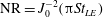 $\text{NR}=J_{0}^{-2}(\unicode[STIX]{x03C0}St_{LE})$
derived by Chaitanya et al. (Reference Chaitanya, Joseph, Narayanan, Vanderwel, Turner, Kim and Ganapathisubramani2017).
$\text{NR}=J_{0}^{-2}(\unicode[STIX]{x03C0}St_{LE})$
derived by Chaitanya et al. (Reference Chaitanya, Joseph, Narayanan, Vanderwel, Turner, Kim and Ganapathisubramani2017).
The above investigations lead to a detailed understanding of the second universal trend of NR growing consistently in the medium-to-high frequency range. The medium-frequency NR (
 $0.5<St_{LE}<2.5$
) is mainly driven by the reduced source magnitude from both the LE and downstream sources as indicated in figure 10(b). It appears that the source phase interference is relatively weaker in the medium frequency range as shown in figure 13 (for
$0.5<St_{LE}<2.5$
) is mainly driven by the reduced source magnitude from both the LE and downstream sources as indicated in figure 10(b). It appears that the source phase interference is relatively weaker in the medium frequency range as shown in figure 13 (for
 $m=16$
). However, as the frequency increases further (
$m=16$
). However, as the frequency increases further (
 $St_{LE}>2.5$
) there is a drastic changeover between the two contributors. The source magnitude contribution falls rapidly (due to the appearance of high-intensity source region downstream of the root in the WLE case as seen in figure 5
c,d), whereas the level of destructive phase interference rises at a faster rate as shown in figure 13 (depicted by the curve fit). This mechanism explains how the noise reduction keeps increasing at the high frequencies.
$St_{LE}>2.5$
) there is a drastic changeover between the two contributors. The source magnitude contribution falls rapidly (due to the appearance of high-intensity source region downstream of the root in the WLE case as seen in figure 5
c,d), whereas the level of destructive phase interference rises at a faster rate as shown in figure 13 (depicted by the curve fit). This mechanism explains how the noise reduction keeps increasing at the high frequencies.
In order to identify the origin of the high level of destructive phase interference appearing at the high frequencies, the real and imaginary parts of
 $\unicode[STIX]{x0394}P_{w}(\boldsymbol{x},f)$
are examined separately,
$\unicode[STIX]{x0394}P_{w}(\boldsymbol{x},f)$
are examined separately,
 $$\begin{eqnarray}\displaystyle \text{Re}(\unicode[STIX]{x0394}P_{w})=|\unicode[STIX]{x0394}P_{w}|\cos \unicode[STIX]{x1D719}\quad \text{and}\quad \text{Im}(\unicode[STIX]{x0394}P_{w})=|\unicode[STIX]{x0394}P_{w}|\sin \unicode[STIX]{x1D719}, & & \displaystyle\end{eqnarray}$$
where
 $$\begin{eqnarray}\displaystyle \unicode[STIX]{x1D719}=-\text{i}\ln \frac{\unicode[STIX]{x0394}P_{w}}{|\unicode[STIX]{x0394}P_{w}|}. & & \displaystyle\end{eqnarray}$$
If there are two different locations where their source magnitudes are equal, i.e.
 $|\unicode[STIX]{x0394}P_{w}|_{1}=|\unicode[STIX]{x0394}P_{w}|_{2}$
, but if they are 180
$|\unicode[STIX]{x0394}P_{w}|_{1}=|\unicode[STIX]{x0394}P_{w}|_{2}$
, but if they are 180
 $^{\circ }$
out of phase, i.e.
$^{\circ }$
out of phase, i.e.
 $\unicode[STIX]{x1D719}_{2}-\unicode[STIX]{x1D719}_{1}=(2n\pm 1)\unicode[STIX]{x03C0}$
, then the values of both
$\unicode[STIX]{x1D719}_{2}-\unicode[STIX]{x1D719}_{1}=(2n\pm 1)\unicode[STIX]{x03C0}$
, then the values of both
 $\text{Re}(\unicode[STIX]{x0394}P_{w})$
and
$\text{Re}(\unicode[STIX]{x0394}P_{w})$
and
 $\text{Im}(\unicode[STIX]{x0394}P_{w})$
at the two locations will have opposite signs. However, they will have the same sign and value if they are in phase, i.e.
$\text{Im}(\unicode[STIX]{x0394}P_{w})$
at the two locations will have opposite signs. However, they will have the same sign and value if they are in phase, i.e.
 $\unicode[STIX]{x1D719}_{2}-\unicode[STIX]{x1D719}_{1}=2n\unicode[STIX]{x03C0}$
. Figure 14 shows the surface contour plots of
$\unicode[STIX]{x1D719}_{2}-\unicode[STIX]{x1D719}_{1}=2n\unicode[STIX]{x03C0}$
. Figure 14 shows the surface contour plots of
 $\text{Re}(\unicode[STIX]{x0394}P_{w})$
and
$\text{Re}(\unicode[STIX]{x0394}P_{w})$
and
 $\text{Im}(\unicode[STIX]{x0394}P_{w})$
calculated at the frequency of
$\text{Im}(\unicode[STIX]{x0394}P_{w})$
calculated at the frequency of
 $St_{LE}=3.5$
, comparing the SLE and WLE cases. It is evident in the figure that the high-intensity sources downstream of the root (in the WLE case) are in fact self-destructive due to the almost perfect out-of-phase relationship taking place between them. A more reasonable measure of the destructive phase interference in the downstream sources may be obtained by calculating SR spectra without the LE sources included. Figure 15 shows the modified phase-based SR spectrum,
$St_{LE}=3.5$
, comparing the SLE and WLE cases. It is evident in the figure that the high-intensity sources downstream of the root (in the WLE case) are in fact self-destructive due to the almost perfect out-of-phase relationship taking place between them. A more reasonable measure of the destructive phase interference in the downstream sources may be obtained by calculating SR spectra without the LE sources included. Figure 15 shows the modified phase-based SR spectrum,
 $\widetilde{\text{SR}}_{phase}(m,f)$
, obtained by calculating contributions from the third segment onward (
$\widetilde{\text{SR}}_{phase}(m,f)$
, obtained by calculating contributions from the third segment onward (
 $j\geqslant 2$
) as follows:
$j\geqslant 2$
) as follows:
 $$\begin{eqnarray}\displaystyle \widetilde{B}_{pw}(m,f)=\left[\mathop{\sum }_{j=2}^{m}A_{pw}(j,f)\right]^{2}\quad \text{and}\quad \widetilde{D}_{pw}(m,f)=\left|\mathop{\sum }_{j=2}^{m}C_{pw}(j,f)\right|^{2}. & & \displaystyle\end{eqnarray}$$
Figure 15 proves that the rapid increase in the destructive phase interference at the high frequencies is generated almost entirely by the downstream sources. This self-destructive mechanism effectively nullifies the downstream source contributions to the far-field sound and therefore allows for maintaining the consistent NR at high frequencies.

Figure 14. Surface contour plots of the real and imaginary parts of
 $\unicode[STIX]{x0394}P_{w}$
at the frequency of
$\unicode[STIX]{x0394}P_{w}$
at the frequency of
 $St_{LE}=3.5$
, comparing the SLE and WLE cases. This figure indicates a high level of destructive phase interference taking place in the strong source region downstream of the root in the WLE case.
$St_{LE}=3.5$
, comparing the SLE and WLE cases. This figure indicates a high level of destructive phase interference taking place in the strong source region downstream of the root in the WLE case.

Figure 15. Phase-based SR (source reduction) spectrum obtained from downstream sources only – integrating from the third segment onward, i.e.
 $j\geqslant 2$
indicated in (5.9). The curve-fit function used is the same as that in figure 13. This figure confirms that the universal trend of NR growing consistently at high frequencies is mainly contributed by destructive phase interference in the downstream sources.
$j\geqslant 2$
indicated in (5.9). The curve-fit function used is the same as that in figure 13. This figure confirms that the universal trend of NR growing consistently at high frequencies is mainly contributed by destructive phase interference in the downstream sources.
6 Conclusion
An in-depth computational study is accomplished in this paper in order to achieve a comprehensive understanding of the noise reduction mechanisms created by WLEs in the event of AVI. One of the crucial findings in this study is that the noise source distribution on the aerofoil surface becomes entirely two dimensional (highly non-uniform in the spanwise direction as well as streamwise) at high frequencies when WLEs are used. Also, it is found that the source magnitude is no longer highest at the leading edge when the frequency reaches a certain point (
 $St_{LE}\approx 3.5$
). This means that the high-frequency noise generation/reduction mechanisms are governed by the downstream sources, which has not before been predicted by using the conventional LE-focused one-dimensional source theories. It is suggested that the strong high-frequency sources created downstream of the WLE are related to asymmetric development of vortical structures between the upper and lower sides of the aerofoil, resulting in a pressure jump across the wall. The full three-dimensional vortex dynamics involved in this process (bisected vortices and their time evolution) has not been detailed in this paper and will be a significant research subject even from purely fluid dynamic perspectives.
$St_{LE}\approx 3.5$
). This means that the high-frequency noise generation/reduction mechanisms are governed by the downstream sources, which has not before been predicted by using the conventional LE-focused one-dimensional source theories. It is suggested that the strong high-frequency sources created downstream of the WLE are related to asymmetric development of vortical structures between the upper and lower sides of the aerofoil, resulting in a pressure jump across the wall. The full three-dimensional vortex dynamics involved in this process (bisected vortices and their time evolution) has not been detailed in this paper and will be a significant research subject even from purely fluid dynamic perspectives.
The investigation of the two-dimensional source characteristics has led to a more complete and correct understanding of the universal trends existing in the frequency spectra of the noise reduction (NR) created by WLEs. Firstly, the negligible level of NR persisting at the low frequencies was in fact due to the conservation of total source energy integrated over the entire aerofoil surface. The surface-integrated source magnitude remained unchanged at the low frequencies regardless of the LE geometry, although locally the source magnitude around the WLE was lower compared to the SLE case. It was found that the surface integration should cover at least
 $4h_{LE}$
downstream of the LE in order to properly address the low-frequency events. Secondly, the rapid and consistent growth of NR at the medium-to-high frequencies was contributed by both the source magnitude reduction and the destructive phase interference but their contribution levels drastically changed with frequency. Again, the inclusion of the downstream sources was crucial for understanding the medium-to-high frequency NR trends. At the medium frequencies (
$4h_{LE}$
downstream of the LE in order to properly address the low-frequency events. Secondly, the rapid and consistent growth of NR at the medium-to-high frequencies was contributed by both the source magnitude reduction and the destructive phase interference but their contribution levels drastically changed with frequency. Again, the inclusion of the downstream sources was crucial for understanding the medium-to-high frequency NR trends. At the medium frequencies (
 $0.5<St_{LE}<2.5$
), the source magnitude reduction was the main driver for NR (with relatively weaker phase interference), contributed fairly equally from the LE and the downstream area. It was then followed by a rapid change of events at the higher frequencies (
$0.5<St_{LE}<2.5$
), the source magnitude reduction was the main driver for NR (with relatively weaker phase interference), contributed fairly equally from the LE and the downstream area. It was then followed by a rapid change of events at the higher frequencies (
 $St_{LE}>2.5$
). There was a strong growth of the source magnitude downstream of the WLE, which was contradictory to the NR trend at the high frequencies. This contradiction was resolved when the source phase interference was investigated. The strong sources generated downstream of the WLE displayed highly self-destructive phase relationships amongst them, resulting in very weak contributions to the radiated sound. This was the high-frequency mechanism that maintained the universal trend of noise reduction.
$St_{LE}>2.5$
). There was a strong growth of the source magnitude downstream of the WLE, which was contradictory to the NR trend at the high frequencies. This contradiction was resolved when the source phase interference was investigated. The strong sources generated downstream of the WLE displayed highly self-destructive phase relationships amongst them, resulting in very weak contributions to the radiated sound. This was the high-frequency mechanism that maintained the universal trend of noise reduction.
The current study was based on an idealised/simplified scenario, i.e. a zero-thickness flat-plate aerofoil, a spanwise-uniform vortex with zero offset from the aerofoil and an inviscid base flow with zero incidence angle. Therefore, there is a long list of variational studies from the current one which may be considered in the future (apart from those that have already been conducted in the existing literature). One of the immediate interests of the authors is to investigate the effect of viscosity on the downstream sources dominant at the high frequencies. One may imagine that there will be significant viscous dissipation (depending on the Reynolds number) on the downstream sources especially at the high frequencies. On the other hand, the highly sheared boundary-layer flow may develop additional vortical structures in the downstream region which might even amplify the downstream sources. These additional nonlinear effects may lead to different outcomes at the high frequencies. Currently, the existing experimental data (that contains viscous effects) are claimed valid up to about
 $St_{LE}\sim 2$
because of other types of noise sources (e.g. self-noise due to turbulent boundary layer scattered at the trailing edge) that might have dominated at the higher frequencies, without clear evidence to it. There is a scope of further work to clarify the high-frequency noise sources.
$St_{LE}\sim 2$
because of other types of noise sources (e.g. self-noise due to turbulent boundary layer scattered at the trailing edge) that might have dominated at the higher frequencies, without clear evidence to it. There is a scope of further work to clarify the high-frequency noise sources.
Acknowledgements
The authors gratefully acknowledge the support of EPSRC (Engineering and Physical Sciences Research Council) under the CDT (Centre for Doctoral Training) grant (EP/G03690X/1) and the ICSS (Institute for Complex Systems Simulation) at the University of Southampton. We would also like to acknowledge the high-performance computing facilities and services of the UK national supercomputer ARCHER via the support of UK Turbulence Consortium (EP/R029326/1), and the local IRDIS4 at the University of Southampton. All data supporting this study are openly available from the University of Southampton repository at doi:10.5258/SOTON/D0912.
Appendix A. Miscellaneous test cases

This appendix section provides additional parametric test cases to support the validity of the current findings, at the request of the reviewers. Firstly, a comparison between the current simulation result (the SLE case) and the classical analytic solution of Amiet (Reference Amiet1975) is provided in figure 16(a). For this purpose we use a two-dimensional version of the analytical solution derived by Blandeau et al. (Reference Blandeau, Joseph, Jenkins and Powles2011), written as
 $$\begin{eqnarray}\displaystyle S_{ppa\text{-}Amiet}(k_{x})=\frac{\unicode[STIX]{x03C0}k_{x}M_{\infty }\unicode[STIX]{x1D70C}_{\infty }^{2}u_{\infty }^{2}L_{c}^{2}\sin ^{2}\unicode[STIX]{x1D703}}{8r_{\!o}A^{3}(\unicode[STIX]{x1D703})}\unicode[STIX]{x1D6F7}_{vv}(k_{x})|{\mathcal{L}}(k_{x})|^{2}, & & \displaystyle\end{eqnarray}$$
where
 $k_{x}=2\unicode[STIX]{x03C0}f/u_{\infty }$
;
$k_{x}=2\unicode[STIX]{x03C0}f/u_{\infty }$
;
 $A(\unicode[STIX]{x1D703})=(1-M_{\infty }^{2}\sin ^{2}\unicode[STIX]{x1D703})^{1/2}$
;
$A(\unicode[STIX]{x1D703})=(1-M_{\infty }^{2}\sin ^{2}\unicode[STIX]{x1D703})^{1/2}$
;
 $r_{o}$
is the observer distance from the mid-chord of the aerofoil;
$r_{o}$
is the observer distance from the mid-chord of the aerofoil;
 $\unicode[STIX]{x1D6F7}_{vv}(k_{x})$
is the PSD of the vertical velocity fluctuations impinging on the LE of the aerofoil; and,
$\unicode[STIX]{x1D6F7}_{vv}(k_{x})$
is the PSD of the vertical velocity fluctuations impinging on the LE of the aerofoil; and,
 ${\mathcal{L}}(k_{x})$
describes the unsteady loading on the aerofoil – see Blandeau et al. (Reference Blandeau, Joseph, Jenkins and Powles2011) for full details. In this paper we apply a semi-infinite-chord approximation (
${\mathcal{L}}(k_{x})$
describes the unsteady loading on the aerofoil – see Blandeau et al. (Reference Blandeau, Joseph, Jenkins and Powles2011) for full details. In this paper we apply a semi-infinite-chord approximation (
 $L_{c}\rightarrow \infty$
) to (A 1) and remove the acoustic backscattering term in
$L_{c}\rightarrow \infty$
) to (A 1) and remove the acoustic backscattering term in
 ${\mathcal{L}}(k_{x})$
in order to obtain the pure LE noise solution (after some algebraic manipulations) as
${\mathcal{L}}(k_{x})$
in order to obtain the pure LE noise solution (after some algebraic manipulations) as
 $$\begin{eqnarray}\displaystyle S_{ppa\text{-}Amiet\text{-}LE}(k_{x})=\frac{\unicode[STIX]{x1D70C}_{\infty }^{2}u_{\infty }^{2}(1-M_{\infty })\sin ^{2}\unicode[STIX]{x1D703}}{2\unicode[STIX]{x03C0}r_{\!o}k_{x}A(\unicode[STIX]{x1D703})^{2}[A(\unicode[STIX]{x1D703})-\cos \unicode[STIX]{x1D703}]}\unicode[STIX]{x1D6F7}_{vv}(k_{x}). & & \displaystyle\end{eqnarray}$$
Figure 16(a) shows a good agreement between the numerical and analytical solutions across all frequencies. In addition, the numerical background noise level that is at least four orders of magnitude lower than the physical noise level at all frequencies is shown in figure 16(b). The background noise level is obtained when the aerofoil (wall boundary condition) is removed from the simulation.

Figure 17. Comparison of the solutions for two different strengths of the impinging vortex:
 $\unicode[STIX]{x1D716}=\unicode[STIX]{x1D716}_{0}$
and
$\unicode[STIX]{x1D716}=\unicode[STIX]{x1D716}_{0}$
and
 $\unicode[STIX]{x1D716}_{0}/2$
where
$\unicode[STIX]{x1D716}_{0}/2$
where
 $\unicode[STIX]{x1D716}_{0}=0.0377$
is the default value used (see § 2.3). (a) Time signals of the acoustic pressure obtained at the observer location specified in figure 2. (b) The corresponding PSD of the former. The pressure is normalised by
$\unicode[STIX]{x1D716}_{0}=0.0377$
is the default value used (see § 2.3). (a) Time signals of the acoustic pressure obtained at the observer location specified in figure 2. (b) The corresponding PSD of the former. The pressure is normalised by
 $\max |p_{a}|_{SLE}$
, i.e. the maximum amplitude of the sound signal from the SLE case.
$\max |p_{a}|_{SLE}$
, i.e. the maximum amplitude of the sound signal from the SLE case.
The second test case is on the effect of different vortex strengths used. Figure 17 shows a comparison of the simulation results obtained from two different vortex strengths, i.e.
 $\unicode[STIX]{x1D716}=0.0377$
(default) and 0.01885 (50 % of the default). The reduced vortex strength provides 50 % weaker induced velocity than the default, i.e.
$\unicode[STIX]{x1D716}=0.0377$
(default) and 0.01885 (50 % of the default). The reduced vortex strength provides 50 % weaker induced velocity than the default, i.e.
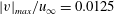 $|v|_{max}/u_{\infty }=0.0125$
(as opposed to 0.025). When the pressure values are normalised by
$|v|_{max}/u_{\infty }=0.0125$
(as opposed to 0.025). When the pressure values are normalised by
 $\max |p_{a}|_{SLE}$
(the maximum amplitude of the sound signal from the SLE case), the two results with different vortex strengths collapse onto each other almost perfectly as shown in figure 17. This indicates that the current findings are well within a linear regime.
$\max |p_{a}|_{SLE}$
(the maximum amplitude of the sound signal from the SLE case), the two results with different vortex strengths collapse onto each other almost perfectly as shown in figure 17. This indicates that the current findings are well within a linear regime.

Figure 18. Re-production of figure 9(b) for two additional cases with different vortex sizes,
 $L_{V}=2L_{V0}$
and
$L_{V}=2L_{V0}$
and
 $2L_{V0}/3$
where
$2L_{V0}/3$
where
 $L_{V0}=1.2\unicode[STIX]{x1D706}_{LE}$
is the default size used (see § 2.3). Here, the dimensionless frequency (Strouhal number) is re-scaled with
$L_{V0}=1.2\unicode[STIX]{x1D706}_{LE}$
is the default size used (see § 2.3). Here, the dimensionless frequency (Strouhal number) is re-scaled with
 $L_{V}/L_{V0}$
to compensate the frequency shift due to the different vortex sizes.
$L_{V}/L_{V0}$
to compensate the frequency shift due to the different vortex sizes.
The third test case is with regard to the effect of different vortex sizes used. Two additional vortex sizes are implemented here:
 $L_{V}/\unicode[STIX]{x1D706}_{LE}=2.4$
(larger) and 0.8 (smaller) where the default size is 1.2 as stated in § 2.3. Figure 18 shows the re-production of figure 9(b) comparing the results from the three different vortex sizes. It is evident from the figure that there is a high level of consistency in the source behaviours despite the significantly different vortex sizes used. Although the larger size case exhibits a slightly delayed appearance of the dominant downstream sources, the other two cases display almost identical results.
$L_{V}/\unicode[STIX]{x1D706}_{LE}=2.4$
(larger) and 0.8 (smaller) where the default size is 1.2 as stated in § 2.3. Figure 18 shows the re-production of figure 9(b) comparing the results from the three different vortex sizes. It is evident from the figure that there is a high level of consistency in the source behaviours despite the significantly different vortex sizes used. Although the larger size case exhibits a slightly delayed appearance of the dominant downstream sources, the other two cases display almost identical results.