


1. Introduction
The flow over an aerofoil undergoing unsteady motion is a difficult phenomenon to predict. Although inviscid models that capture the trailing wake physics of an unsteady aerofoil (Theodorsen Reference Theodorsen1935; Sears Reference Sears1938; Greenberg Reference Greenberg1947) have been developed, a low-order representation of viscous flow mechanisms, particularly the formation of large-scale vortical structures, remains elusive. The leading-edge vortex (LEV) is one such vortical structure that causes significant discrepancies in force production compared to conventional aerodynamic theories (Eldredge & Jones Reference Eldredge and Jones2019). The LEV has been investigated at length in a number of fundamental studies regarding surging, pitching and rotating flat plates (Ellington et al. Reference Ellington, van den Berg, Willmott and Thomas1996; Birch & Dickinson Reference Birch and Dickinson2001; Kriegseis, Kinzel & Rival Reference Kriegseis, Kinzel and Rival2013; Mancini et al. Reference Mancini, Manar, Granlund, Ol and Jones2015; Panah, Akkala & Buchholz Reference Panah, Akkala and Buchholz2015; Manar Reference Manar2018), and its growth has been successfully modelled for cases where the timing of vortex formation is known beforehand (Wang & Eldridge Reference Wang and Eldridge2013; Wong & Rival Reference Wong and Rival2015; Manar & Jones Reference Manar and Jones2019). In more realistic flows, however, the question of when flow separation occurs becomes a driving factor in understanding LEV formation. For an arbitrary unsteady motion, the rounded leading edge of an aerofoil supports a finite pressure gradient, and unlike the case of a flat plate, flow separation is not guaranteed at the leading edge of the wing throughout its motion. The current work seeks to understand the onset of LEV formation on an aerofoil with a rounded leading edge and focuses on a set of motion kinematics where the timing of flow separation is a significant unknown.
When approaching this topic, one must first recognize that an LEV forms on an aerofoil over a broad range of unique and complex flow environments. On a helicopter in forward flight, for instance, the blades of the main rotor are subject to a time-varying free-stream velocity, a time-varying pitch angle and a spanwise-varying flap velocity, all of which can contribute to the formation of an LEV. Many researchers have thus approached separated aerofoil flows by decomposing real-world environments into a series of simple unsteady motions. One particularly well-known motion is the case of an aerofoil undergoing pitch oscillations in a constant free stream, a configuration that has been studied extensively over the past several decades (Carr, McAlister & McCroskey Reference Carr, McAlister and McCroskey1977; Beddoes Reference Beddoes1979; McCroskey Reference McCroskey1982; Lorber & Carta Reference Lorber and Carta1988). Collectively, these works define the basic stages of LEV formation on a pitching aerofoil and address the sensitivity of the aerofoil's aerodynamic forces to variations in pitching kinematics. Their observations have also provided a physical basis for many predictions of aerofoil flow separation (McAlister, Lambert & Petot Reference McAlister, Lambert and Petot1984; Leishman & Beddoes Reference Leishman and Beddoes1989; Deparday & Mulleners Reference Deparday and Mulleners2019). It must be kept in mind, however, that the insights obtained from these works, and especially any empirical modelling techniques, are limited to the subset of aerofoil kinematics where the pitching motion is the dominant unsteady effect. In most practical applications, flow separation occurs in an environment where numerous other unsteady features significantly impact the timing of LEV formation, meaning methods for predicting the timing of flow separation on a pitching aerofoil are not strictly valid.
More recent efforts have sought to expand the understanding of separated aerofoil flows to cases where the free-stream velocity is time varying (Choi, Colonius & Williams Reference Choi, Colonius and Williams2015; Granlund, Ol & Jones Reference Granlund, Ol and Jones2016; Kocher et al. Reference Kocher, Cummings, Tran and Sahni2017; Kirk & Jones Reference Kirk and Jones2018). Of particular note, Dunne & McKeon (Reference Dunne and McKeon2015) considered the case of a NACA 0018 wing undergoing a simultaneous surging and pitching manoeuvre. Mirroring the periodic nature of a vertical-axis wind-turbine blade, the authors implemented the following oscillatory motion as a way of introducing the impact of free-stream variance on LEV formation
 \begin{equation} U(t) = U_0 \left( 1+\lambda \sin(\varOmega t) \right), \end{equation}
where  $\varOmega$ represents the frequency of the oscillation,
  $U_0$ represents a mean free-stream velocity and
  $\lambda$ represents the amplitude of the free-stream oscillation. The authors performed an extensive modal decomposition of the resulting flow field measurements and linked the time scales of flow separation to the frequency of the free-stream oscillation (Dunne, Schmid & McKeon Reference Dunne, Schmid and McKeon2016). A series of similar efforts have also been performed that characterize the force production and flow field evolution on a surging and pitching aerofoil under various surge amplitudes, frequencies and phase shifts relative to the pitching kinematics (Gharali & Johnson Reference Gharali and Johnson2013; Wang & Zhao Reference Wang and Zhao2016; Gharali et al. Reference Gharali, Gharaei, Soltani and Raahemifar2018; Medina et al. Reference Medina, Ol, Greenblatt, Muller-Vahl and Strangfeld2018). Although a promising step forward in understanding vortex formation on aerofoils in more realistic aerodynamic environments, each of these studies focuses on a set of aerofoil kinematics where the surge amplitude is less than
  $\lambda = 1$. The portion of the parameter space where
  $\lambda > 1$ is a unique flow regime, as the amplitude of the free-stream oscillation is large enough that the aerofoil passes through a free-stream velocity of
  $U(t) = 0$ during its deceleration, but it has yet to be studied in a fundamental context. This regime also represents a reasonable approximation of many real-world flow scenarios, including the inboard elements of a high-speed helicopter shown to exhibit flow separation during the deceleration (or ‘retreating’) portion of their oscillation cycle (Lind et al. Reference Lind, Trollinger, Manar, Chopra and Jones2018), and the blades of vertical-axis wind turbines when encountering low tip speed ratios (Parker & Leftwich Reference Parker and Leftwich2016).
The current work seeks to experimentally investigate the onset of LEV formation in this high-amplitude surge regime. The overall goal is to understand how the various mechanisms of flow separation, particularly unsteady effects, impact the timing of vortex formation on a high amplitude surging/pitching wing. The following sections will introduce the experimental methodology, provide a qualitative overview of LEV formation on a surging and pitching wing and investigate how a change in surge amplitude and frequency impacts the timing of LEV formation. A final section will demonstrate how these observations apply to the field of low-order aerodynamics modelling by explicitly predicting the timing of vortex formation on a surging and pitching wing with a mixture of potential flow and boundary layer theory.
2. Methodology
2.1. Theoretical approach
Before diving into the details of the current experimental set-up, it is first important to establish what specific physical mechanisms impact the timing of flow separation, and how the expected behaviour of these mechanisms informs our approach. Figure 1 provides a basic sketch of an aerofoil undergoing an arbitrary surging and pitching manoeuvre. Flow separation is triggered at the leading edge of this aerofoil when the pressure gradient (or surface acceleration) becomes excessively large and adverse. The factors that influence flow separation can thus be described based on how they impact the local pressure gradient and the fluid momentum in a region near the leading edge of the wing.

Figure 1. Problem statement: an aerofoil with a rounded leading edge is subject to an unsteady free-stream velocity ( $U(t$)) and incidence (
 $\alpha (t$)). The onset of flow separation is seen as a function of (1) the instantaneous wing kinematics, (2) the velocity induced by the trailing wake and (3) unsteady effects in the boundary layer.
The first mechanism in figure 1 is the steady contribution of the instantaneous incidence ( $\alpha (t$)) and free stream (
 $U(t$)). These instantaneous kinematics determine the manner in which the bulk flow is accelerated over the surface of the wing and account for a significant portion of the suction peak near the leading edge. In terms of flow separation, an increase in incidence (
 $\alpha (t$)) increases the velocity gradient near the leading edge, which leads to a larger adverse pressure gradient relative to the flow momentum. Likewise, an increase in free stream leads to an increase in the instantaneous Reynolds number, which is associated with a thinner boundary layer, a larger shear stress at the wing surface, and a delay in the onset of flow separation. The steady contribution can thus be seen as a function of the relative magnitude of the adverse pressure gradient (controlled by the instantaneous angle of attack) and the height of the boundary layer (controlled by the instantaneous Reynolds number).
The second mechanism sketched in figure 1 is the unsteady contribution of the aerofoil's trailing wake. When an aerofoil undergoes an unsteady manoeuvre, its bound circulation becomes a function of time, and the aerofoil must shed circulation into its wake to uphold Kelvin's theorem. As a result, the aerofoil is trailed throughout its motion by a rotational region of the flow field. This region induces a velocity back on the surface of the wing and can have a significant impact on the magnitude of the pressure gradient. In a general, an acceleration leads to a trailing wake that decreases the relative magnitude of the pressure gradient near the leading edge, delaying the onset of flow separation, while a deceleration results in an increased pressure gradient near the leading edge, promoting the onset of flow separation.
The final mechanism sketched in figure 1 is the presence of unsteady acceleration effects within the boundary layer. Although the wake contribution accounts for unsteadiness in the ‘external’ flow, fluid particles within the boundary layer experience an additional mechanism of separation because of their proximity to an accelerating wall. Stated another way, an accelerating boundary introduces the notion of a ‘Stokes layer’ into the overall boundary layer structure, and the need to maintain a finite acceleration at the wall can significantly impact the curvature of the resulting boundary layer profile. With this in mind, an acceleration of the wing will generally delay separation, simply by imparting a forward momentum to the fluid particles near the wall, while a deceleration will promote separation.
Altogether, figure 1 identifies three mechanisms that govern the timing of flow separation: (1) the instantaneous incidence and Reynolds number, (2) the velocity induced by the trailing wake and (3) unsteady effects in the boundary layer. The current work aims to understand the relative importance of each of these mechanisms in the process of flow separation on a surging and pitching aerofoil, with a specific focus on the more seldom-studied unsteady effects. To accomplish this task, flow field measurements were collected on a pitching aerofoil undergoing a series of free-stream oscillations, each with a different surge amplitude and reduced frequency. The pitching kinematics and mean Reynolds number were held constant in each case, with the intent of minimizing changes to the steady flow field contribution. The next section will describe how these flow field measurements were obtained, before beginning an intensive analysis of the flow fields themselves.
2.2. Experimental set-up
Flow field measurements were collected on a NACA0012 wing ( $c = 0.115\ \mathrm {m}$,
  $AR = 4$) in a
  $7\ \mathrm {m} \times 1.5\ \mathrm {m} \times 1 \ \mathrm {m}$ free-surface water-filled tow tank located at the University of Maryland. Figure 2 shows a photograph of the tow tank (a) and a simple sketch of the mounting apparatus used to position the aerofoil beneath the tank's free surface (b). This apparatus is connected via two control rods to a magnetic track and gantry. The presence of the mounting apparatus, together with the finite aspect ratio of the wing, means that the flow will not be entirely two dimensional; however, force and flow field measurements in the same test facility have compared well with strictly two-dimensional (2-D) models of attached (Kirk & Jones Reference Kirk and Jones2018) and separated flows (Manar & Jones Reference Manar and Jones2019). These past results suggest that three-dimensionality, while certainly present, is expected to have a small impact on the large-scale flow structures studied in the current experiments.

Figure 2. Photograph (a) and sketch (b) of the experimental set-up and water-filled tow tank facility.
During each experimental run, a double-pulsed, Nd:YLF laser (Litron LDY304, 30 mJ, 10 kHz max) illuminated a planar region located one chord from the centreline of the wing. Simultaneously, a high-speed camera (Phantom v641, 4 Mpx, 1450 f.p.s. max) was mounted to the gantry and captured a wing-fixed field of view. The laser and camera were operated such that a minimum of 800 images were collected over the deceleration portion of the wing's surge manoeuvre, equivalent to a sampling rate in the range of 250–500 Hz. The exact value of the sampling rate was dependent on the specific reduced frequency of the run, and it remained constant throughout the oscillation. Note that all flow field measurements were phase averaged over six successive runs of the experiment. The convergence properties of the phase-averaging process will be briefly addressed in later sections of this work.
Figure 3 provides a sample particle image (a) and processed vorticity field (b) to highlight the resolution of the resulting flow measurements. Each flow field image extends roughly 255 mm (or 2.2 chords) in the horizontal direction and 162 mm (or 1.4 chords) in the vertical direction. The images were cross-correlated with an interrogation window that achieved  $215\times 137$ vectors over our field of view, corresponding to roughly 97 vectors per chord length, while a portion of the flow below the wing was obscured by the presence of a laser shadow. A laser reflection, visible in the left-hand side of figure 3, further obscured a thin region on the upper surface of the aerofoil, but this reflection appears much smaller than the height of the aerofoil boundary layer, meaning it is unlikely to affect the flow field statistics introduced later in our analysis.

Figure 3. Sample particle image (a) and phase-averaged vorticity field (b) for the baseline surging and pitching condition of the aerofoil.
The surging kinematics used in this study take the same basic form as those in (1.1). A slightly modified, more illustrative version of this expression can be written as follows:
 \begin{equation} U(t) = U_0 \Big[1 + \lambda \sin \left(2kt^{*} \right) \Big],\end{equation}
where the new parameter  $k$ represents the reduced frequency of the surge oscillation (
 $k = \varOmega c / 2U_0$) and
  $t^{*}$ represents the convective time (
 $t^{*} = t U_0/c$). Equation (2.1) provides a simple way of visualizing the relationship between the instantaneous surge velocity and the non-dimensional properties of the oscillation. The surge amplitude
  $\lambda$ controls the maximum and minimum velocity achieved during the oscillation, the reduced frequency
  $k$ controls the amount of convective time required to complete the oscillation (but does not affect the range of velocities achieved), and the mean velocity
  $U_0$ sets an average Reynolds number (
 $Re_0 = U_0 c / \nu$) for the motion. All three parameters (
 $\lambda$,
  $k$, and
  $U_0$) directly scale the maximum acceleration experienced by the aerofoil during its oscillation. In the sections that follow, a parameter space encompassing the surge amplitude (
 $1.50 \leq \lambda \leq 2.25$) and the reduced frequency (
 $0.1 \leq k \leq 0.3$) will be explored in regard to the timing of flow separation, while the mean Reynolds number will be held constant at
  $Re_0 = 2 \times 10^{4}$.
A dynamic pitching motion was introduced at the same time as the surging oscillation for each run of the experimental set-up. The pitching kinematics were again oscillatory in nature and can be represented by the following simple relation:
 \begin{equation} \alpha(t) = \alpha_0 + \alpha_1 \sin \left(\frac{2kU_0}{c} t + \phi \right) \end{equation}
where  $\alpha _0$ represents a mean pitch angle,
  $\alpha _1$ represents a pitch amplitude and
  $\phi$ is a phase shift relative to the surging motion. Each of these three pitching parameters was held constant (
 $\alpha _0 = 15^{\circ }$,
  $\alpha _1 = 8^{\circ }$,
  $\phi = {\rm \pi}$) for all cases as a way of isolating the role of an unsteady free-stream velocity. The exact values of the mean pitch angle and amplitude were chosen to ensure that the flow remained attached over some portion of the wing's surging and pitching oscillation; that is, because the angle of attack varies over the range
  $7^{\circ } \leq \alpha \leq 23^{\circ }$, the flow can neither be assumed to be attached or separated throughout the entire oscillation. A constant phase shift of
  $\phi = {\rm \pi}$ was chosen to mirror the environment of a helicopter in forward flight, where rotor blades are typically pitched up during their deceleration as a way of maintaining a stable roll moment, and the wing pitching axis was set at the aerofoil quarter-chord (
 $c/4$), again inspired by a conventional helicopter blade in forward flight.
Figures 4, 5 and 6 summarize the surging and pitching kinematics that will be investigated in the following sections. In these figures, the motion kinematics of each test case are plotted against a non-dimensional cycle time, defined as  $\psi = \varOmega t$, which will be used to identity each phase of the pitching/surging cycle. Note that in figure 5, the four reduced frequency cases collapse to a single line when plotted with
  $\psi$, but each case is performed at an increasing large value of the dimensional frequency
  $\varOmega$.

Figure 4. Surging kinematics for each of the four surge amplitude cases.

Figure 5. Surging kinematics for each of the four reduced frequency cases.

Figure 6. Pitching kinematics for the current work.
3. Results
This section aims to assess the role of an unsteady free-stream velocity in the process of vortex formation on a combined surging and pitching wing. In §§ 3.1 and 3.2, the stages of vortex formation, and the relevant flow field statistics, are introduced for a baseline set of surging/pitching kinematics. In §§ 3.3 and 3.4, the baseline kinematics are perturbed, and the timing of LEV formation is investigated over a variety of reduced frequencies ( $0.1 \leq k \leq 0.3$) and surge amplitudes (
 $1.50 \leq \lambda \leq 2.25$). Section 3.5 introduces a novel, computationally quick method for predicting the onset of flow separation based on the physical conclusions gathered throughout this work.
3.1. Flow morphology
Figure 7 presents a series of flow field snapshots that illustrate the basic stages of vortex formation for the baseline surge ( $\lambda = 1.75$,
  $k = 0.165$) and pitch condition (
 $\alpha _0 = 15^{\circ }$,
  $\alpha _1 = 8^{\circ }$,
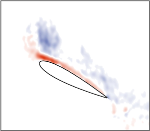
  $\phi = {\rm \pi}$) of the aerofoil. Each snapshot is overlain with contours of counter-clockwise vorticity (red) and clockwise vorticity (blue). The flow fields in figure 7 were measured over the range
  $160^{\circ } < \psi < 270^{\circ }$, which captures a significant portion of the wing's pitch-up motion, the period over which a vortex is expected to form at the blunt edge of the wing. Note that each snapshot only includes measurements of the wing's upper surface, while the underside is masked due to a laser shadow.

Figure 7. Basic stages of LEV formation for the baseline kinematics ( $\lambda = 1.75$,
  $k = 0.165$,
  $\alpha _0 = 15^{\circ }$,
  $\alpha _1 = 8^{\circ }$). The aerofoil exhibits stages of (1) attached flow, (2) separation near the leading edge, (3) vortex rollup and (4) vortex shedding.
Figure 7 identifies several unique stages of vortex formation on a surging and pitching wing. At flow snapshot (1), for instance, the instantaneous velocity and pitch angle are at their mean values, and no appreciable flow separation is observed on the surface of the wing. The height of the boundary layer appears quite large, but the vorticity within this region is all of the same sign and roughly follows the surface of the blade. Flow field snapshot (2) corresponds to  $\psi \approx 200^{\circ }$ and provides the first evidence of flow separation. A shear layer has emerged at the leading edge of the wing, and a region of counter-clockwise vorticity can be seen beneath the shear layer, indicating that the sign of the local shear stress has reversed. The shear layer feeds an LEV until shortly after the aerofoil passes through
  $U(t) = 0$, an event represented by snapshot (3), at which point the LEV appears to have been ‘pinched off’ from the surface of the wing. In flow field snapshot (4), the wing has transitioned fully into a period of free-stream reversal, and the LEV has begun to convect in the direction of the free stream.
3.2. Flow field statistics
In many ways, the flow evolution described in figure 7 is similar to the canonical stages of LEV formation found throughout the literature: flow separates near the leading edge, a shear layer forms and the LEV is fed by the shear layer until it is shed from the wing. The main differences are that (a) the flow in figure 7 remains mostly attached until nearly midway through its oscillation cycle and (b) the ‘pinch off’ of the LEV appears to coincide with the reversal of the free-stream velocity, rather than the LEV reaching some critical size. The overall goal of this work is to understand the physics of (a), or to arrive at a reasonable prediction of the time at which flow near the leading edge is no longer attached. This goal can be aided by a direct, quantitative estimation of when the LEV begins its formation, a measurement that takes advantage of the unique properties of the flow morphology outlined in figure 7.
To illustrate the calculation of LEV initiation, consider the following equation, which relates the growth rate of the LEV to its final strength
 \begin{equation} \varGamma_f = \int_{t_{i}}^{t_{f}} \left(\frac{\mathrm{d}\varGamma(t)}{\mathrm{d} t} \right) \mathrm{d}t, \end{equation}
where  $\varGamma _f$ is the final strength of the LEV after being shed from the wing;
  $t_{i}$ is the time at which vortex formation and growth begins;
  $t_{f}$ is the time at which vortex growth ends; and
  $\mathrm {d}\varGamma /\mathrm {d}t$ represents the time-resolved growth rate of the LEV. Equation (3.1) is useful in the sense that it can be manipulated to isolate the time at which vortex formation begins (
 $t_i$) and the remaining terms can be approximated by simple flow field statistics.
The growth rate of the LEV ( $\mathrm {d}\varGamma /\mathrm {d}t$), for instance, can be captured by considering the shear layer at the rounded edge. Figure 7 illustrated that the LEV is fed by this shear layer throughout its growth stage. The growth rate of the LEV can thus be determined by calculating the instantaneous flux of vorticity in the shear layer at each time step. The right-hand side of figure 8 shows a simple control volume used to accomplish this task. As the LEV forms, its growth rate is represented by the flux of clockwise (blue) vorticity out of this control volume, which is assumed to be equivalent to the flux of vorticity into the LEV. The left-hand side of figure 8 shows the result of this flux measurement for the wing at its baseline surging and pitching kinematics. Over the period of vortex formation, the growth rate of the LEV is found to be a monotonically decreasing function in time, reaching a value of zero shortly before the wing's passage through
  $U(t) = 0$. This figure also reveals that the measurement of vorticity flux, and thus the growth rate of the LEV, is well converged when 6 runs are included in the phase-averaging process.

Figure 8. The flux of clockwise (blue) vorticity measured at the leading edge of the wing throughout the baseline case. Note that this measurement is shown with an increasing number of runs included in the phase-averaging process.
The final strength of the LEV ( $\varGamma _f$) can be computed in a similar fashion. Figure 7 revealed that after the end of its growth stage, the LEV convects with the local flow velocity in the direction of the ‘reversed’ free stream, to the left of the wing's rounded edge. The right-hand side of figure 9 sketches a vertical flux plane located in the path of the LEV's convection. If one were to compute the flux of clockwise vorticity through this flux plane, the convection of the LEV would appear as a prolonged spike in the value of vorticity flux over time. The left-hand side of figure 9 provides an example of the LEV's signature on the vorticity flux, and illustrates how this measurement behaves over successive runs of the experimental set-up. The current work uses a temporal integration of this ‘spike’, the bounds of which are denoted as 10 % of the maximum flux, as a reasonable estimation of the total clockwise vorticity contained within the LEV. Again, the peak and bounds are this spike appear to be relatively invariant when four or more runs are included in the phase-averaging process, providing confidence that we are indeed measuring an LEV with repeatable strength and convection properties.

Figure 9. Illustration of the calculation of final vortex strength  $\varGamma _f$. A flux plane is drawn beyond the rounded edge of the wing, and the LEV strength is determined by integrating the flux of clockwise (blue) vorticity through this plane.
The only remaining terms in (3.1) are the bounds of the integration, or the time at which vortex growth begins ( $t_i$) and the time at which it ends (
 $t_f$). The flow morphology of figure 7 suggest that the end of LEV growth can be assumed to coincide the timing of free-stream reversal, as the reverse flow region was observed to ‘cut off’ the growth of the vortex. If
  $t_f$ is replaced by
  $t_{rev}$ in (3.1),
  $t_i$ becomes the sole unknown, and (3.1) can be rearranged to isolate the time at which vortex formation begins. This process, wherein the onset of vortex formation (
 $t_i$) is estimated based on the vortex growth rate (
 $\mathrm {d}\varGamma /\mathrm {d}t$) and final vortex strength (
 $\varGamma _f$), is employed in the following sections to determine the timing of vortex formation for each set of surging/pitching kinematics. Note that vorticity annihilation, which has been suggested as an important mechanism of LEV growth on rotating wings (Wojcik & Buchholz Reference Wojcik and Buchholz2014; Medina & Jones Reference Medina and Jones2016), was found to be insignificant in the measurements described above, likely because the LEV is only close to the aerofoil surface for a short period prior to free-stream reversal.
3.3. Variation in reduced frequency
Our analysis will begin by investigating how a change in the reduced frequency ( $k$) impacts the timing of vortex formation on a combined surging and pitching wing. From a physics standpoint, the reduced frequency is an intuitive place to begin, as a change in reduced frequency changes the wing acceleration while keeping the instantaneous velocity and pitching kinematics constant (see figure 5). A change in the reduced frequency is thus expected to manifest solely as a change in strength of the trailing wake and unsteadiness in the boundary layer. This section is intended to illuminate the role that these unsteady mechanisms play in triggering the onset of vortex formation.
Figure 10 plots the timing of vortex formation ( $\psi _{vor}$), computed using the methodology outlined in § 3.2, over a sweep of reduced frequencies (
 $0.1 \leq k \leq 0.3$). For each point in figure 10, the surge amplitude (
 $\lambda = 1.75$) and pitching kinematics (
 $\alpha _0 = 15^{\circ }$,
  $\alpha _1 = 8^{\circ }$,
  $\phi = {\rm \pi}$) were held constant, such that the steady contribution to the flow field was expected to be identical in each case. The acceleration of the wing, in contrast, triples over the range
  $0.1 \leq k \leq 0.3$, meaning the unsteady mechanisms of separation, namely the wake and unsteady boundary layer contributions, should see a significant change in magnitude.

Figure 10. The effect of reduced frequency ( $k$) on the timing of vortex formation (
 $\psi _{vor}$) for a constant surge amplitude (
 $\lambda = 1.75$) and set of pitching kinematics (
 $\alpha _0 = 15^{\circ }$,
  $\alpha _1 = 8^{\circ }$,
  $\phi = {\rm \pi}$).
Figure 10, however, reveals a rather unexpected result. Despite the large range of accelerations experienced over  $0.1 \leq k \leq 0.3$, the timing of vortex formation appears relatively insensitive to changes in the reduced frequency. The physical reason for this insensitivity is not immediately obvious; that is, it is unclear whether unsteady effects have a low overall magnitude, or whether they interact in such a way that their effects negate one another. The remainder of this section will explore the behaviour of the unsteady mechanisms of flow separation, specifically the velocity induced by the trailing wake and unsteady effects the boundary layer, in the hopes of explaining the trends observed in figure 10.
3.3.1. Trailing wake effects
The trailing wake is main feature of the ‘external’ flow field affected by change in oscillation frequency. For higher reduced frequencies, the wing completes its oscillation in less convective time, and the circulation in the trailing wake has less time to convect away from the surface of the wing. The trailing wake is thus expected to induce a larger velocity at the surface of the wing at higher values of the reduced frequency due to the closer proximity of trailing vorticity.
The velocity induced by the wake cannot be measured directly, but its magnitude can be seen as proportional to certain properties of the wake. Figure 11 provides a sketch of a rectangular control volume located a short distance ( $c/4$) from the wing's trailing edge. In the current work, this control volume is assumed to represent the bounds of the ‘near wake’, or the portion of the wake with the most significant impact on the velocity induced on the wing surface. The strength of the near wake, and thus the relative magnitude of the wake-induced velocity, can be estimated by performing a simple area integral of all clockwise (blue) and counter-clockwise (red) vorticity contained within the control volume and comparing the resulting strength among the various values of reduced frequency.

Figure 11. Illustration of the control volume used to estimate the strength of the near wake.
Figure 12 plots the strength of the near wake ( $\varGamma _w$) for each of the four reduced frequency cases, during the portion of the oscillation that immediately precedes the onset of flow separation. If the wake-induced velocity was in fact changing significantly with the reduced frequency, the strength of the near wake would be expected to undergo a similar change in its magnitude. Figure 12, however, reveals that the strength of the near wake, and in turn the velocity induced by the wake, is largely insensitive to changes in the reduced frequency. This does not mean that the velocity induced by the wake is small, but it does imply that an increase in reduced frequency from
  $k = 0.1$ to
  $k = 0.3$ is not enough to significantly impact the pressure gradient near the leading edge. We can conclude that a major reason for the insensitivity of
  $\psi _{vort}$ to reduced frequency is that the state of the trailing wake, and the velocity it induces near the leading edge, is only a weak function of the reduced frequency over the range
  $0.1 \leq k \leq 0.3$.

Figure 12. The effect of reduced frequency ( $k$) on the strength of the near wake (
 $c/4$ beyond the trailing edge) at constant surge amplitude (
 $\lambda = 1.75$).
3.3.2. Unsteady boundary layer effects
The presence of unsteadiness within the boundary layer, or unsteadiness due an accelerating wall, is an additional mechanism of separation whose magnitude is expected to have a strong link to the reduced frequency. Similar to the classical Stokes boundary layer, the acceleration of the wing imparts its own momentum on fluid particles close to the aerofoil boundary, and can play a significant role in separation if the acceleration magnitude is sufficiently high (Dwyer & McCroskey Reference Dwyer and McCroskey1971; Riley Reference Riley1975). The insensitivity of  $\psi _{vor}$ with reduced frequency, together with the invariance of the wake seen in figure 12, imply that acceleration effects in the boundary layer are negligible over the range
  $0.1 \leq k \leq 0.3$, but it is nonetheless important to establish an upper bound at which acceleration effects become significant in the surging/pitching wing problem, as this has important ramifications for the modelling efforts undertaken later in this work.
Such an upper bound can be established by leveraging figure 10 with the expected magnitude of unsteadiness in the boundary layer. Equation (3.2) provides a non-dimensional form of the incompressible boundary layer equation, which governs the magnitude of the various mechanisms at play near the aerofoil surface
 \begin{equation} \left(\frac{L}{T U}\right) \frac{\partial u^{*}}{\partial t^{*}} + u^{*} \frac{\partial u^{*}}{\partial x^{*}} + v^{*} \frac{\partial u^{*}}{\partial y^{*}} = -\frac{\partial p^{*}}{\partial x^{*}} + \frac{\partial^{2} u^{*}}{\partial (y^{*})^{2}}. \end{equation}
In (3.2),  $T$ is a characteristic time scale,
  $U$ is a characteristic velocity,
  $L$ is a characteristic velocity scale and the terms marked with a ‘
 $*$’ are all approximately of
  $O(1)$. ‘Internal’ unsteady effects are represented by the first term on the left hand side of (3.2), with a magnitude dependent on the flow's characteristic length, time and velocity.
A number of these characteristic scales can be quite easily related to kinematics of the surging and pitching wing problem. The velocity scale  $U$, for instance, is likely of the same order of magnitude as the aerofoil free-stream
  $U(t)$, while the time constant
  $T$ likely scales with the inverse of the oscillation frequency (
 $1/\varOmega$). Both of these selections are consistent with classical steady and unsteady boundary layer theory (Schlichting Reference Schlichting2017). The length scale
  $L$, in contrast, is less clearly defined. A typical selection for
  $L$ would be the airfoil chord, which leads to the unsteady term scaling with twice the reduced frequency
 \begin{equation} \frac{L}{T U}= \frac{\varOmega c}{U(t)} = 2k. \end{equation}
Although this leads to a simple relation between unsteady effects and the aerofoil kinematics, (3.3) suggests that unsteady effects are comparable in magnitude to the pressure gradient over the range  $0.1 \leq k \leq 0.3$, meaning that both mechanisms should play a significant role in the structure of the boundary layer. Such an observation is inconsistent with the insensitivity of
  $\psi _{vort}$ to reduced frequency observed in figure 10.
An alternate approach would be to set the characteristic length scale  $L$ equal to the distance of a given point from stagnation. This parameter, denoted here as
  $x$, is inherently related to the height of the boundary layer and appears in a number of fundamental analytical solutions to the boundary layer equations. This selection also means that the unsteady term is scaled according to a very intuitive non-dimensional parameter, defined as follows:
 \begin{equation} \frac{L}{T U} = \frac{\varOmega x}{U} = \left(\frac{\nu x}{U} \right) \left(\frac{\varOmega}{\nu} \right) = \left(\frac{\delta}{\delta_s}\right)^{2}.\end{equation}
 In (3.4),  $\delta$ is the order of the local boundary layer height (
 $\delta = (\nu x/U)^{1/2}$), while
  $\delta _s$ is the expected height of the Stokes layer (
 $\delta _s = (\nu / \varOmega )^{1/2}$). The Stokes layer effectively represents the height of the boundary layer if acceleration were the only mechanisms influencing the boundary layer structure, or if the problem were idealized to an accelerating infinite flat plate. The parameter in (3.4) can thus be seen as a measure of how far the current boundary layer flow deviates from the idealized case of an accelerating plate. If
  $\varOmega x/U$ is much less than
  $O(1)$, for instance, the Stokes layer is expected to be large compared to the actual boundary layer height, and unsteady effects are unlikely to be significant at the scales relevant to the boundary layer. In contrast, if
  $\varOmega x/U$ is
  $O(1)$ or greater, the Stokes layer is expected to be comparable to the actual height of the boundary layer, and unsteady effects become significant.
With this in mind, figure 13 plots the scaling parameter from (3.4) for our four reduced frequencies in the period immediately preceding the onset of flow separation. To generate each line, the parameter  $x$ was set to
  $0.1 c$, a conservative estimate of the distance between stagnation and the point of leading-edge separation. Figure 13 reveals that the behaviour of
  $\varOmega x/U$ is consistent with the relation between
  $\psi _{vor}$ and
  $k$; that is, this scaling law predicts a very low magnitude of acceleration effects in the boundary layer, even after the reduced frequency is tripled from its base value. It also allows us to establish an upper bound at which time-acceleration effects in the boundary layer are expected to become a significant factor in the onset of flow separation: based on the trends in figure 13, unsteady boundary layer effects appear likely to remain small as long as
  $k$ remains below
  $O(10)$. For reference, most practical applications, including helicopter and wind turbine aerodynamics, generally feature reduced frequencies of
  $O(1)$ or lower.

Figure 13. The expected magnitude of time-acceleration effects in the boundary layer relative to the contribution of viscosity and the pressure gradient (both of which are assumed to be  $O(1)$ in this figure) at constant surge amplitude (
 $\lambda = 1.75$).
As a brief summary, this section found that the timing of vortex formation has a weak dependence on the reduced frequency. Over the range  $0.1 \leq k \leq 0.3$, a change in the reduced frequency did not manifest as a significant change in the strength of the near wake, nor did it give any indication of significant unsteadiness in the boundary layer. Based on a simple scaling analysis, the preceding conclusion is expected to hold as long as the reduced frequency
  $k$ is of
  $O(1)$ or lower; higher reduced frequencies (i.e.
  $k > 1$) are expected to result in non-negligible unsteadiness within in the boundary layer.
3.4. Variation in surge amplitude
The next stage of this analysis will investigate how a change in the surge amplitude ( $\lambda$) impacts the timing of vortex formation on a surging and pitching wing. Similar to the reduced frequency, a change in the surge amplitude corresponds to a change in the acceleration of the aerofoil, and is thus expected to manifest as a change in the properties of the trailing wake and the boundary layer. The main difference is that a change in surge amplitude also impacts the range of instantaneous velocities experienced by the aerofoil during its oscillation; the ‘steady’ contribution to the flow field cannot be assumed constant across multiple surge amplitude. This section will explore the effects of surge amplitude in terms of the steady contribution, the unsteady contribution, and their mutual interaction, in the hopes of illuminating the main physical mechanisms linked to a change in amplitude.
To begin, figure 14 shows the onset of vortex formation ( $\psi _{vor}$) as it changes with surge amplitude (
 $\lambda$) for a constant reduced frequency (
 $k = 0.165$) and set of pitching kinematics (
 $\alpha _0 = 15^{\circ }$,
  $\alpha _1 = 8^{\circ }$,
  $\phi = {\rm \pi}$). This figure displays a very clear trend; the onset of vortex formation occurs at progressively earlier times in the oscillation cycle for increasing values of the surge amplitude. The intuition behind this assertion is straightforward (i.e. a more aggressive surge manoeuvre leads to earlier flow separation), but the physical mechanisms responsible for this trend are not immediately apparent. It is unclear whether figure 14 can be attributed to (i) a simple change in the instantaneous kinematics, (ii) unsteady acceleration effects in the boundary layer or (iii) changes in the structure of the trailing wake. The remainder of this section will walk through each mechanism individually and assess whether or not it can account for the trend in figure 14.

Figure 14. The effect of surge amplitude ( $\lambda$) on the timing of vortex formation (
 $\psi _{vor}$) at constant reduced frequency (
 $k = 0.165$) and pitching kinematics (
 $\alpha _0 = 15^{\circ }$,
  $\alpha _1 = 8^{\circ }$,
  $\phi = {\rm \pi}$).
3.4.1. Quasi-steady contribution
Let us begin with the steady effects brought about by changing the instantaneous kinematics in each surge amplitude case. Referring to the kinematics in figure 4, the higher surge amplitude cases reach a lower instantaneous free stream, and thus a lower instantaneous Reynolds number, at earlier times in the oscillation cycle compared to the lower surge amplitude cases. From a steady perspective, a lower instantaneous Reynolds number is associated with a thicker boundary layer, and a thicker boundary layer is more prone to an early flow separation. The ‘steady’ perspective would predict that the trends in figure 14 are simply due to the higher amplitudes reaching lower Reynolds numbers at earlier times.
It is unclear, however, whether this steady contribution alone is enough to account for the trends seen in figure 4. One way to quantify the relative impact of steady effects is to consider the height of the boundary layer near the leading edge in the moments leading up to the onset of flow separation. If steady effects are truly responsible for the change in  $\psi _{vort}$ with
  $\lambda$, the boundary layer height should increase significantly at higher values of the surge amplitude, as these cases reach lower Reynolds numbers at earlier times.
With this in mind, boundary layer measurements were computed for each surge amplitude case over the range  $170^{\circ } \leq \psi \leq 185^{\circ }$. The process consisted of identifying a point near the leading edge of the wing, drawing a line outward from the surface of the wing, and interpolating for the vorticity along that line. The ‘edge’ of the boundary layer was defined as the point at which the local vorticity decreased below a ‘threshold’ value of
  $\omega _0 = 2.5 U_0/c$. The current work performs this calculation at 4 different points over the range
  $0.1 \leq x/c \leq 0.15$, then averages the resulting heights at each time step, ultimately arriving at a smooth approximation of the leading edge boundary layer height over time. A sample vorticity distribution, corresponding to the
  $x/c = 0.12$ at
  $\psi = 182^{\circ }$, is provided in figure 15 for the baseline surging and pitching case.

Figure 15. The distribution of vorticity along a line normal to the  $c/10$ chordwise position on the aerofoil suction surface. The white dot represents the ‘edge’ of the boundary layer. Note that this profile is taken from the baseline case (
 $\lambda = 1.75$,
  $k = 0.165$) at
  $\psi = 182^{\circ }$.
Figure 16 presents measurements of the height of the boundary layer ( $\delta$) over the portion of the aerofoil motion that immediately precedes separation. Despite the different instantaneous Reynolds numbers experienced by each surge amplitude, the lines in figure 16 all behave in a similar fashion, with no clear trend in the boundary layer height. There are small variations among the cases, but the magnitude of these variations are within the spatial resolution of the flow field measurements (0.0103 chords), meaning they are likely a result of experimental noise. The main takeaway of figure 16 is thus that the height of the boundary layer is quite invariant with surge amplitude over the parameter space of interest.

Figure 16. The effect of surge amplitude ( $\lambda$) on the instantaneous height of the boundary layer at a position roughly
  $c/10$ from the leading edge of the wing.
We conclude that the steady contribution to separation, or the notion that lower instantaneous Reynolds numbers leads to an earlier separation, cannot completely account for the trends in figure 14. This conclusion makes intuitive sense; a meaningful change in the height of the boundary layer would likely only begin to be noticed once the instantaneous Reynolds number is reduced by a full order of magnitude, which for the current parameter space, occurs after the flow has already separated.
3.4.2. Unsteady boundary layer effects
Next, we will address the relation between the surge amplitude and unsteadiness within the boundary layer, or the effects of an accelerating wall. Since a change in the surge amplitude leads directly to a change in the aerofoil acceleration, the magnitude of time-acceleration effects in the boundary layer are expected to scale with the surge amplitude; however, much like the reduced frequency, it can be shown through a simple scaling analysis that unsteady boundary layer effects are negligible for realistic values of the surge amplitude. Figure 17 plots the expected magnitude of the unsteady term, formally introduced in § 3.3, for a variety of surge amplitudes in the moments that immediately precede flow separation. Each line retains a very small magnitude throughout the oscillation, even with a conservative estimate for the length scale ( $x = 0.1 c$), suggesting that time-acceleration effects are negligible in the overall structure of the boundary layer. We conclude, via a simple scaling law, that ‘internal’ unsteady effects in the boundary layer play a small role in the timing of flow separation (assuming that
  $\lambda$ and
  $k$ are both of
  $O(1)$ or less).

Figure 17. The expected magnitude of time-acceleration effects in the boundary layer relative to the contribution of viscosity and the pressure gradient (both of which are assumed to be  $O(1)$ in this figure) at constant reduced frequency (
 $k = 0.165$).
3.4.3. Trailing wake effects
At this stage, our analysis has concluded that neither quasi-steady effects (i.e. the change in instantaneous Reynolds number) nor unsteady boundary effects (i.e. changes in the boundary layer structure due to an accelerating wall) can sufficiently explain the inverse relationship between  $\lambda$ and
  $\psi _{vort}$ observed in figure 14. The remaining mechanism of the flow is the influence of the trailing wake. This section will outline why the velocity induced by the wake, and specifically its magnitude relative to the instantaneous velocity of the aerofoil, is the most likely explanation for the trends seen in figure 14.
To begin, figure 18 plots the strength of the near wake against non-dimensional time, again computed using the control volume approach of § 3.3. Despite the different accelerations imposed by each amplitude, figure 18 shows a weak relation between  $\lambda$ and the strength of the wake. This observation simply implies that the change in acceleration from
  $\lambda = 1.50$ to
  $\lambda = 2.25$ is not enough to significantly affect the circulation shed into the wake; however, it also implicitly points to a unique interaction between the wake and the instantaneous free stream.

Figure 18. The effect of surge amplitude ( $\lambda$) on the strength of the near wake (
 $\varGamma _w$) for four surge amplitudes at constant reduced frequency and pitching kinematics.
Consider, for example, two cases from figure 18, one case at the lowest surge amplitude ( $\lambda = 1.50$) and another case at a highest surge amplitude (
 $\lambda = 2.25$). The flow near the leading edge in both cases can be roughly broken down into a ‘quasi-steady’ component due to the instantaneous surge/pitch motion (
 $U_1$ and
  $U_2$) and an ‘unsteady’ component due to the trailing wake (
 $U_w$). In dimensional form, figure 18 suggests that
  $U_w$ is approximately the same for
  $\lambda = 1.50$ and
  $\lambda = 2.25$; the quasi-steady component, in contrast, is lower for
  $\lambda = 2.25$ when
  $\psi > 180^{\circ }$. The higher surge amplitude case is thus subject to a higher effective incidence, which then leads to an earlier onset of flow separation. This process, wherein a lower instantaneous free-stream velocity results in an earlier flow separation, is illustrated in figure 19 and is valid as long as flow separation occurs after the wing passes through
  $\psi = 180^{\circ }$.

Figure 19. Illustration of how the wake-induced velocity, which is reasonably constant across the four surge amplitudes, increases the effective incidence near the leading edge.
To summarize, this section found that an increase in the surge amplitude  $\lambda$ results in an earlier onset of vortex formation over the range
  $1.50 \leq \lambda \leq 2.25$. This phenomenon could not be attributed to ‘quasi-steady’ effects (i.e. the notion that higher surge amplitudes reach lower instantaneous Reynolds numbers at earlier times in the oscillation) nor ‘internal’ unsteady effects in the boundary layer (i.e. effects due the accelerating wall), leaving only the influence of the trailing wake. Through direct measurements of its strength, the trailing wake was shown to increase the effective incidence near the leading edge of the aerofoil at higher surge amplitudes, which the current work posits as the most reasonable explanation for the trends in vortex formation seen in figure 14.
3.5. Low-order prediction of vortex formation
Taken together, the preceding sections have uncovered a few important observations regarding the physics of flow separation on a surging and pitching aerofoil. The velocity induced by the trailing wake appears to drive an earlier flow separation at higher surge amplitudes, while unsteadiness within the boundary layer appears to be small for practical values of the reduced frequency and surge amplitude. These conclusions have important ramifications for the prediction of vortex formation on a surging and pitching wing. This section will revisit how vortex formation is typically predicted in popular low-order models, and will attempt to identify further reductions of order based on the conclusions noted above.
As a bit of background, low-order models of unsteady flows generally consist of two components. The first is a model of the inviscid flow outside the boundary layer, which range from conventional source/vortex panel methods (Hess Reference Hess1990; Katz & Plotkin Reference Katz and Plotkin2001) to those rooted in complex potential flow theory (Milne-Thompson Reference Milne-Thompson1938; Wang & Eldridge Reference Wang and Eldridge2013). The second is a viscous treatment of the rotational flow that occurs within the boundary layer, which is typically handled by an ‘integral’ method of solving the steady or unsteady boundary layer equations (Lock & Williams Reference Lock and Williams1987; Cebeci et al. Reference Cebeci, Platzer, Hang and Chen1993; Ramos-Garcia, Sorensen & Shen Reference Ramos-Garcia, Sorensen and Shen2014). Because of nonlinearities in the boundary layer equations, these integral methods are too computationally expensive for use in many design scenarios, especially those that deal with unsteady flows. It has thus become an important goal of the unsteady aerodynamics community to find an alternate boundary layer method that quickly and accurately computes the onset of vortex formation in an unsteady environment.
Perhaps the most popular of these low-order methods is the leading-edge suction parameter, or ‘LESP’ for short. The LESP is based on the hypothesis that a given airfoil can support a finite amount of suction before experiencing massive flow separation at its leading edge, and its validity has been explored over a range of airfoil geometries and unsteady motions (Ramesh et al. Reference Ramesh, Gopalarathnam, Granlund, Ol and Edwards2012, Reference Ramesh, Gopalarathnam, Granlund and Ol2014, Reference Ramesh, Granlund, Ol, Gopalarathnam and Edwards2017). In practice, the LESP is ideal for low-order predictions of vortex formation, as it manifests as a simple check for separation at the leading edge, but it remains somewhat limited in the types of flow it can accurately predict. The ‘critical’ value of the LESP, for instance, is believed to be different for each individual combination or aerofoil and Reynolds number, which makes it non-ideal for use in design scenarios where the aerofoil geometry undergoes multiple iterations.
The current work proposes an alternate criterion for vortex formation, one based on the observations of §§ 3.3 and 3.4, that improves upon some of the limitations of the LESP. Consider, as a starting point, the governing equations of the boundary layer for a 2-D surging and pitching aerofoil, stated formally as follows:
 \begin{equation} \frac{\partial u}{\partial t} + u\frac{\partial u}{\partial x} + v\frac{\partial u}{\partial y} = \left(\frac{\partial U_e}{\partial t} + U_e \frac{\partial U_e}{\partial x} \right) + \nu \frac{\partial^{2} u}{\partial y^{2}}. \end{equation}
In (3.5),  $u$ and
  $v$ are velocity components within the boundary layer,
  $U_e$ is the exterior velocity of the boundary layer (obtained from the inviscid outer flow) and
  $x$ and
  $y$ are the directions tangent and normal to the aerofoil surface.
As discussed above, the methods for directly solving (3.5) are still too computationally expensive for use in many applications. At this stage, we will make a few reasonable assumptions to simplify (3.5) into a more mathematically convenient form. First, the unsteady term (represented by  $\partial u/ \partial t$) can be removed from (3.5) since ‘internal’ time-acceleration effects were found to be negligible over the parameter space of interest. This assumption is expected to be valid as long as the reduced frequency
  $k$ is
  $O(1)$ or lower. Likewise, we will assume that the boundary layer at the leading edge is locally self-similar, meaning that the magnitude of the
  $u ({\partial u}/{\partial x})$ term near the surface is small compared to the pressure gradient. This is expected to be a reasonable assumption given the very large magnitude of the pressure gradient characteristic of flows with a leading-edge separation. Together, these two assumptions lead us to the well-known Falkner–Skan formulation of the boundary layer equations, stated as follows:
 \begin{equation} f_{\eta \eta \eta} + f f_{\eta \eta} + \beta \left(1-f_{\eta}^{2} \right) = 0. \end{equation}
In (3.6),  $f$ is a transformed version of the streamfunction in the boundary layer,
  $\eta$ is the scaled wing-normal direction and
  $\beta$ is non-dimensional representation of the local pressure gradient. This equation is a ‘single-parameter’ ordinary differential equation and is among the simplest iterations of the boundary layer equations. A solution for shear stress at the surface, and thus a prediction for the timing of flow separation, can be ascertained based only on the single parameter
  $\beta$, which is itself a function of the inviscid slip velocity at a certain point along the aerofoil surface (
 $\beta = ({1}/{U_e}) ({\partial U_e}/{\partial x}$)). Solutions to (3.6) have been documented for various values of the non-dimensional pressure gradient throughout the literature, and the value of
  $\beta \approx -0.1988$ has been analytically found to correspond to the onset of flow separation.
The Falkner–Skan equation represents a simple, first-order approximation of when the vortex formation process begins on an aerofoil in an unsteady flow, but it is important to recognize that such an approach is only strictly valid for a laminar boundary layer. The presence of turbulence, which becomes increasingly significant at higher Reynolds numbers, plays a major role in energizing the boundary layer and maintaining flow attachment. The current work, taking inspiration from the LESP, posits that the influence of turbulence manifests as a change in the ‘critical’ value of the Falkner–Skan parameter  $\beta$. That is, for a turbulent boundary layer, separation occurs at a magnitude higher (i.e. more negative) than
  $\beta = -0.1988$, and this specific value depends only on the mean Reynolds number of the aerofoil motion.
To illustrate this idea, figure 20 plots the maximum magnitude of  $\beta$, computed using an unsteady version of the Hess–Smith panel method for a NACA 0012 (Hess Reference Hess1990), for each of the four surge amplitude cases. The maximum adverse value of the Falkner–Skan parameter (
 $\beta _{max}$) is seen to monotonically increase for each case in figure 20, leading up to the experimentally measured timing of vortex formation (denoted with a blue dot). More importantly, figure 20 shows that
  $\beta _{max}$ is roughly constant at the onset of vortex formation, with
  $\psi _{vor}$ occurring at roughly
  $\beta _{max} = -2.1$ for each case. The onset of leading-edge separation thus appears to coincide with a critical value of the Falkner–Skan parameter, with the presence of turbulence increasing the magnitude of this critical value above the laminar point of laminar separation (
 $\beta _{max} = -0.1988$).

Figure 20. The value of the maximum non-dimensional pressure gradient ( $\beta _{max}$) computed in a region near the leading edge (
 $0 \leq x/c \leq 0.25$) for a NACA 0012 over various surge amplitudes.
In a similar vein, figure 21 applies this idea to the trends in vortex formation with surge amplitude (a) and reduced frequency (b). For each set of kinematics, the inviscid outer flow was predicted with a simple unsteady panel method, and the timing of flow separation was predicted based on the value of the Falkner–Skan parameter near the leading edge. The results of this prediction are plotted as solid black dots in figure 21, while the experimental measurements are plotted as blue dots. The critical value of the Falkner–Skan parameter was set to  $\beta _{max} = -2.1$ for each case, as there is no change in the mean Reynolds number of the aerofoil motion. The left-hand side of figure 21, which corresponds to the sweep in surge amplitude, shows very good agreement between the experimental measurement and the prediction of vortex formation, with both the magnitude and trends in
  $\psi _{vor}$ being well represented. The right-hand side shows that the method is also successful at capturing the insensitivity of
  $\psi _{vor}$ to changes in reduced frequency, although it has a slight error in magnitude.

Figure 21. The predicted timing of vortex formation ( $\psi _{vor}$) compared to experimental measurement for a sweep of surge amplitudes (
 $\lambda$, a) and reduced frequency (
 $k$, b).
As a final comment, we will also note that there is a strong resemblance between the method outlined above and the more well-known leading-edge suction parameter. In both methods, one computes the inviscid flow outside the boundary layer using an unsteady panel method, then checks some leading-edge flow property against a critical value that corresponds to flow separation. The main difference is that the critical value of the Falkner-Skan parameter, since it is based firmly in boundary layer theory, is not expected to vary with aerofoil geometry. The influence of geometry is largely captured by the inclusion of  $\partial U_e/ \partial x$, and by explicitly changing the aerofoil shape in the inviscid step. It is only the influence of turbulence that needs to be handled empirically. The critical value of the Falkner–Skan parameter should then only depend on the mean Reynolds number of the aerofoil motion, making it more versatile in the way it approaches vortex formation.
4. Conclusions
The formation of a leading-edge vortex on a conventional aerofoil is a difficult process to understand and predict. Although numerous works have addressed the growth and shedding stages of LEV development on flat plates, it remains unclear how to predict the transition from attached to separated flow on a wing with a rounded leading edge, a critical event in many external flow applications. In this work, a series of experimental flow field measurements were used to investigate the mechanisms responsible for flow separation on a simultaneously surging and pitching aerofoil at high surge amplitudes ( $\lambda$) and reduced frequencies (
 $k$). The exact surging and pitching kinematics were chosen to be perfectly out-of-phase with one another to mirror the unsteady free stream and pitch oscillations observed in rotary wing applications. Experiments focused on the impact of the free-stream oscillation and consisted of a sweep four surge amplitudes (
 $1.50 \leq \lambda \leq 2.25$) and four reduced frequencies (
 $0.1 \leq k \leq 0.3$). The following conclusions were reached:
(i) For a surging/pitching aerofoil with a phase difference of
 $\phi = {\rm \pi}$, leading-edge flow separation was consistently found to occur during the pitch-up/deceleration portion of the aerofoil's motion, leading to the formation of a strong vortex at the blunt leading edge.
(ii) When the surge amplitude exceeded
$\lambda = 1$, a period of free-stream reversal was present in the wing's surging kinematics and acted to ‘cut off’ the growth of the LEV. As a result, the LEV convected beyond the blunt edge of the aerofoil as the wing continued to surge in reverse flow.(iii) The onset of vortex formation was found to be insensitive to the reduced frequency over the range
$0.1 \leq k \leq 0.3$. The reason for this insensitivity was assessed in relation to trailing wake effects and ‘internal’ acceleration effects. A large change in reduced frequency had little effect on the strength of the near-wake over $0.1 \leq k \leq 0.3$, meaning the wake-induced velocity remained reasonably constant over a large range of reduced frequencies. Likewise, the magnitude of unsteadiness within the boundary layer was addressed through a scaling analysis and was found to be an order of magnitude smaller than the leading-edge pressure gradient. It was predicted that unsteady boundary layer effects would be negligible in the onset of vortex formation as long as $k$ is of $O(1)$ or lower, which was supported by the trend in the timing of vortex formation with reduced frequency.(iv) The onset of vortex formation was found to occur at earlier times in the oscillation cycle with increasing surge amplitude. This was attributed to an increase in the relative strength of the aerofoil's trailing wake at higher values of the surge amplitude. Again, unsteady effects in the boundary layer were determined to be quite small in this regime, with a low order of magnitude compared to the local pressure gradient at separation.
(v) The timing of flow separation in both the surge amplitude and reduced frequency sweeps was well predicted by a simple combination of an inviscid panel method and a quasi-steady treatment of the boundary layer equations. This reinforces the notion that unsteady boundary layer effects are negligible in the regime studied here. Likewise, by using the computationally inexpensive Falkner-Skan equation, a novel shedding criterion was proposed based on a ‘critical’ value of the Falkner–Skan parameter (
$\beta = ({1}/{U_e}) ({\partial U_e}/{\partial x}$)) in a region near the leading edge. The ‘critical’ value of this parameter is expected to be independent of aerofoil geometry, varying only with the degree of turbulence in the boundary layer, and provides a promising avenue for future efforts in modelling the onset of LEV formation.


Acknowledgements
This work was supported by the U.S. Army/Navy/NASA Vertical Lift Research Center of Excellence Cooperative Agreement with M. Bhagwat serving as Program Manager and Technical Agent, grant number W911W6-17-2-0004.
Declaration of Interests
The authors report no conflict of interest.


