


1. Introduction
In many porous rocks, large-scale heterogeneities lead to preferential flow paths which can have a dominant impact on the transport by flow through the porous layer. A variety of approaches have been used to describe the associated dispersion (Greenkorn & Kessler Reference Greenkorn and Kessler1969; Matheron & De Marsily Reference Matheron and De Marsily1980; Dagan Reference Dagan1982; Srzic et al. Reference Srzic, Cvetkovic, Andricevic and Gotovac2013; Kampman et al. Reference Kampman, Bickle, Maskell, Chapman, Evans, Purser, Zhou, Schaller, Gattacceca and Bertier2014). Many are based on the assumption that the heterogeneities become decorrelated over some length scale, beyond which the transport becomes Fickian, while at earlier times, the transport may be anomalous owing to correlations in the velocity field (Koch & Brady Reference Koch and Brady1988; Berkowitz, Scher & Silliman Reference Berkowitz, Scher and Silliman2000; Zavala-Sanchez, Dentz & Sanchez-Vila Reference Zavala-Sanchez, Dentz and Sanchez-Vila2009).
With heterogeneities of finite scale, in an unbounded zone the dispersion does eventually become Fickian. A simple approach to demonstrate this result was developed by Eames & Bush (Reference Eames and Bush1999) building on the work of Cala & Greenkorn (Reference Cala and Greenkorn1986), who followed the travel times on different streamlines passing through or around a localised zone of different permeability. Eames and Bush developed this approach for flow through an array of elliptical shaped zones of heterogeneity, and determined expressions for the effective Fickian dispersivity. The approach has since been generalised by Dagan & Lessoff (Reference Dagan and Lessoff2001), Lessoff & Dagan (Reference Lessoff and Dagan2001), Dagan & Fiori (Reference Dagan and Fiori2003) and Fiori, Janković & Dagan (Reference Fiori, Janković and Dagan2003) for a variety of structures of the heterogeneity, and the results have been tested with detailed numerical simulations (Janković, Fiori & Dagan Reference Janković, Fiori and Dagan2003). Curiously, in developing this work further, Darvini (Reference Darvini2016) and Rabinovich, Dagan & Miloh (Reference Rabinovich, Dagan and Miloh2012) found that if there is a random distribution of heterogeneities in a porous channel with impermeable boundaries, then as well as the Fickian dispersion, a shear develops in the average along-channel velocity near the boundary. Rabinovich et al. (Reference Rabinovich, Dagan and Miloh2012) developed expressions for the effective permeability near the boundary for both two- and three-dimensional flow.
Given that many natural rocks include such heterogeneities, in this paper we further explore the impact of this effective shear on the transport in a bounded heterogeneous porous layer. First, we present a simple model of the origin of the boundary shear in a channel, bounded above and below by impermeable rock, and which includes a series of long, thin rectangular shaped heterogeneities at random positions across the channel. We then develop a layer-averaged model for the dispersion of tracer in such a medium, including the effect of the shear and the Fickian dispersivity. We also develop some asymptotic solutions showing that, at long times, the shear leads to elongation of the tracer at a rate proportional to  $t$ rather than the earlier time Fickian spreading proportional to
  $t^{1/2}$. We then demonstrate similar results for the case of elliptically shaped zones of heterogeneity, building from the approach of Eames and Bush. We discuss the possible impact of these results for tracer tests in laterally extensive, vertically confined permeable layers as may be deployed in the assessment of reservoir connectivity for carbon capture and storage applications. We note that this shear is distinct from that described by Matheron & De Marsily (Reference Matheron and De Marsily1980), who showed that, with a series of parallel layers of different permeability, tracer spreads out proportional to time
  $t$; physically, that effect is related to the differing speed of the flow in the different layers.
2. Development of shear flow in a bounded domain
We consider an idealised pressure-driven flow through a layer of permeable rock of permeability  $k_1$ which contains a series of lenses of permeability
  $k_2$ located at different random positions across the channel. We assume that the lenses are long and thin, with length
  $l$ in the along-flow direction and height
  $h$ in the cross-flow direction, while the channel has width
  $H$ such that
  $l \gg H,h$. The lenses are placed in series so that the horizontal distance between the edges of successive lenses is much greater than the width of the channel,
  $(L-l) \gg H$.
It may be shown that for such a configuration, where there is a lens, the flow above and below the centre of the lens partitions into two parallel streams, with a fraction  $\mathcal {F} = k_2 h/(k_2 h + k_1 (H-h))$ in the lens, and a fraction
  $1-\mathcal {F}$ outside the lens (figure 1a,b; cf. Phillips Reference Phillips2009; Woods Reference Woods2015). For a random location of the centre of the lens, the probability
  $\mathcal {P}(z)$ that a streamline at height
  $z$ in a uniform part of the channel passes through the lens depends on whether
  $\mathcal {F}<1/2$ or
  $\mathcal {F}>1/2$, and is given by
 \begin{equation} \mathcal{P}(z) = \begin{cases} \displaystyle\frac{z}{1-\mathcal{F}} & \text{for} \ z \leq \mathcal{F},\\ \displaystyle\frac{\mathcal{F}}{1-\mathcal{F}} & \text{for} \ \mathcal{F} \leq z \leq 1-\mathcal{F},\\ \displaystyle\frac{1-z}{1-\mathcal{F}} & \text{for} \ z \geq 1-\mathcal{F}. \end{cases} \end{equation}
for  $\mathcal {F}<1/2$. Similarly, for
  $\mathcal {F}>1/2$,
  $\mathcal {P}(z)$ is given by
 \begin{equation} \mathcal{P}(z) = \begin{cases} \displaystyle\frac{z}{1-\mathcal{F}} & \text{for} \ z \leq 1-\mathcal{F},\\ 1 \quad & \text{for} \ 1-\mathcal{F}\leq z \leq \mathcal{F},\\ \displaystyle\frac{1-z}{1-\mathcal{F}} & \text{for} \ z \geq \mathcal{F}.\end{cases} \end{equation}
This is shown in figure 1(c). The probability varies across the channel since streamlines in the centre of the channel are more likely to be diverted into the lens, since they can move upwards or downwards, while those near the boundary are constrained by the boundary (figure 1a,b).

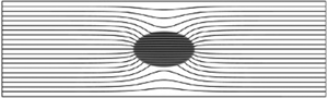
Figure 1. (a,b) The streamlines for the flow past a long and thin rectangular lens with permeability greater than the background permeability ( $k_2/k_1=10, l=15, h=0.05, H=1$), located with its centre at
  $z_c=0.25$ and
  $z_c=0.025$ respectively. In each case, the lens diverts approximately 7 of 21 streamlines across the channel, as indicated in blue. (c) For an assemblage of lenses in the channel, the probability,
  $\mathcal {P}(z)$, that a streamline at height
  $z$ goes through a lens is shown as a function of height
  $z$ for different values of the fractional flow,
  $\mathcal {F}$, through each lens. The three profiles shown in panel (c) correspond to
  $\mathcal {F}=0.4,0.5,0.6$ for the cases
  $\mathcal {F}<1/2$,
  $\mathcal {F}=1/2$ and
  $\mathcal {F}>1/2$ respectively.
If the centres of the lenses are a distance  $L$ apart, and the lenses have length
  $l(<L)$, then, if the flow speed is
  $u_{\infty }$ in a uniform part of the channel and
  $Q$ is the total flux of fluid moving through the channel, the travel time along a streamline in moving a distance
  $L$ between the mid-point of the gaps between successive lenses is
 \begin{equation} t_i = \frac{l\left( k_1 (H-h)+k_2h \right)}{k_iQ} + \frac{L-l}{u_{\infty}} \quad \text{for}\ i=1,2, \end{equation}
where  $i=2$ or
  $i=1$ depending on whether the streamline passes through the lens or is diverted around the lens (figure 1a,b). In this simple picture, we neglect the details of the involved in the adjustment of the flow between regions of uniform permeability and regions including lenses since
  $L-l, l \gg H$. In appendix B we show this is a good approximation, using a full two-dimensional simulation of the flow (appendix A).
If there are a series of lenses down the channel with their centres located at the points  $x_c(\,j)=(2j-1)L/2$ for
  $j=1,\ldots ,n$ (
 $L > l$), but at a series of random vertical positions across the channel, then in passing through
  $n$ lenses, there are
  $(n+1)$ possible travel times along a streamline originally at height
  $z$ in a uniform part of the channel, depending on the number of lenses that the streamline passes through. These travel times, given by
  $nt_2, ((n-1)t_2 + t_1), ((n-2)t_2 + 2t_1),\ldots ,nt_1$, have probabilities given by the terms in the binomial expansion of
  $( \mathcal {P}(z)+(1-\mathcal {P}(z)) )^n$.
In the limit of large  $n$ (appendix C) this binomial distribution of travel times converges to a normal distribution for
  $0 < \mathcal {P} < 1$, so that the travel time distribution is given by
 \begin{equation} \text{TTD}(x=nL,z,t) = \frac{1}{\sqrt{2{\rm \pi} n \sigma_t^2(z)}} \exp \left( \frac{(t-nt_m(z))^2}{2 n \sigma_t^2(z)} \right), \end{equation}
where the mean travel time,  $t_m(z)$, and the variance of travel time,
  $\sigma _t^2(z)$, are given by (cf. (2.3))
 \begin{equation} t_m(z) = t_2 \mathcal{P}(z) + t_1 (1-\mathcal{P}(z)), \quad \sigma_t^2(z) = (t_2 - t_1)^2\mathcal{P}(z)(1-\mathcal{P}(z)). \end{equation}
 Since  $\mathcal {P}$ varies across the channel, we see that the mean speed also varies across the channel, and this leads to the net shear in the flow associated with the boundaries. Following the work of Levenspiel & Smith (Reference Levenspiel and Smith1957), we expect that the tracer concentration can be expressed in terms of the along-channel-averaged conservation equation,
 \begin{equation} c_t + U(z) c_x = D(z) c_{xx}, \end{equation}
where the mean flow,  $U(z)$, and longitudinal dispersion coefficient,
  $D(z)$, are given by (cf. (2.5a,b))
 \begin{equation} U(z) = \frac{L}{t_m(z)} \quad \text{and} \quad D(z) = \frac{1}{2} L^2 \frac{\sigma_t ^2(z)}{t_m^3(z)}, \end{equation}
provided that  $x =nL \gg D/U$, which requires that
 \begin{equation} n \gg \frac{\sigma_t^2(z)}{2t_m^2(z)} \gg \frac{(t_2 - t_1)^2\mathcal{P}(z)(1-\mathcal{P}(z))}{2(t_2 \mathcal{P}(z) + t_1 (1-\mathcal{P}(z)))^2}. \end{equation}
 Figure 2 shows the profiles of mean speed,  $U(z)$, and longitudinal dispersion coefficient,
  $D(z)$ (2.7a,b), for a range of values of permeability ratio,
  $k_2/k_1$, and width ratio,
  $h/H$, of the lens to the channel. Note that
  $k_2/k_1<1$ represents lenses with permeability lower than the background permeability, which we refer to as low permeability lenses, and
  $k_2/k_1>1$ represents high permeability lenses. Figures 2(c)–2(\,f) illustrate that the shear becomes stronger as either (i) the magnitude of the permeability contrast between the lens and the background is increased, or (ii) as the cross-layer width of the lens relative to the channel increases, since this leads to a greater fractional flow through the lens. On the other hand, for a low permeability lens (
 $k_2/k_1<1$), the fractional flow through the lens is a small fraction of the net flow, and so the probability,
  $\mathcal {P}(z)$, is nearly constant across the channel except in a narrow region near the top and bottom boundaries, where there is a narrow region of shear (figure 2a,b).

Figure 2. Case  $l/H=10$,
  $L=2l=20$. The profiles of mean speed,
  $U(z)$, and dispersion coefficient,
  $D(z)$ (see (2.7a,b)), for a range of values of permeability ratio,
  $k_2/k_1$, and width ratio,
  $h/H$, of the lens to the channel. Panels (a,b) correspond to low permeability lenses with
  $h/H=0.1$. Panels (c,d) correspond to high permeability lenses with
  $h/H=0.05$. Panels (e,\,f) correspond to high permeability lenses with
  $k_2/k_1=10$ and varying width ratio
  $h/H$.
A pulse of tracer of unit volume injected instantaneously into the fluid at  $t=0$, (2.6) has a well-known solution
 \begin{equation} c(x,z,t) = \frac{c_o}{2 \sqrt{{\rm \pi} D(z) t}} \exp \left(- \frac{(x-U(z)t)^2}{4D(z)t}\right). \end{equation}
 Equations (2.9) and (2.4) are analogous once the flow has advanced sufficiently far so that  $x \gg D/U$ (see (2.8)). We therefore use profiles of mean speed,
  $U(z)$, and longitudinal dispersion coefficient,
  $D(z)$, to describe the transport of tracer as it passes through an assemblage of lenses. Although
  $c(x,z,t)$ strictly represents the probability distribution of the arrival of tracer at a particular point in space and time, we refer to
  $c(x,z,t)$ as the concentration of tracer. Figures 3(a)–3(d) show the predicted transport of a pulse of tracer along a channel after it has moved through
  $1, 10, 100$ and
  $1000$ lenses, respectively, according to (2.9).

Figure 3. Case  $k_2/k_1=10$,
  $h/H=0.05$,
  $l/H=10$. (a–d) The tracer concentration,
  $c(x,z,t=nL/\bar {U})$, is shown here at four times after its initial release at
  $x=0$,
  $t=0$, after it has passed through
  $n=1,10,100,1000$ lenses, respectively. The red dotted line shows the mean along-channel position of tracer, which is advection driven with speed
  $U(z)$. Panels (e–h) show the corresponding depth-averaged profiles,
  $\bar {c}(x,t=nL/\bar {U})$.
3. Layer-averaged model for tracer transport
We define the layer-averaged concentration,
 \begin{equation} \bar{c}(x,t) = \frac{1}{H}{\int_0^H c(x,z,t)\,\mathrm{d}z}. \end{equation}
 Figures 3(e)–3(h) show this layer-averaged concentration profile corresponding to the distribution of tracer shown in figures 3(a)–3(d). Based on these layer-averaged profiles, we have estimated the mean position of the centre of mass of tracer,  ${x}_m(t)$, and the variance of longitudinal extent of the tracer, relative to the mean,
  $\sigma ^2(t)$, as
 \begin{equation} {x}_m(t) = \frac{\displaystyle\int_{-\infty}^\infty \bar{c}(x,t) x \,\mathrm{d}x} {\displaystyle\int_{-\infty}^\infty \bar{c}(x,t) \,\mathrm{d}x}, \quad \sigma ^2(t) = \frac{\displaystyle\int_{-\infty}^\infty \bar{c}(x,t) (x-x_m(t))^2 \,\mathrm{d}x} {\displaystyle\int_{-\infty}^\infty \bar{c}(x,t)\,\mathrm{d}x}. \end{equation}
 Figure 4(a) illustrates the evolution of the standard deviation of the tracer,  $\sigma$, with time,
  $t$. At early times,
  $\sigma$ grows as
  $t^{1/2}$ but at late times, the spreading of tracer becomes controlled by the effective mean shear and grows linearly with time
  $t$. We define
  $\hat {D}$ by fitting the curve
  $\sigma \approx (2 \hat {D} t)^{1/2}$ to the numerical data at early times (dispersion-controlled regime), while at late times, we define
  $\hat {U}$ by fitting the curve
  $\sigma \approx \hat {U}t$ (shear-controlled regime) (figure 4a). We expect the transition from the early to the long time regime to be given by a transition time,
  $\tau$, which is found by matching the early time and late time solutions,
  $\tau = 2\hat {D}/{\hat {U}}^2$. Using the properties of the mean flow and dispersion at each height in the channel, we can define the following quantities
 \begin{equation} \Delta U ^2 = \frac{1}{H}{\int_0^H (U(z) - \bar{U})^2\,\mathrm{d}z}, \quad \bar{U} = \frac{1}{H}{\int_0^H U(z)\,\mathrm{d}z},\quad \bar{D} = \frac{1}{H}{\int_0^H D(z)\,\mathrm{d}z}. \end{equation}
Figure 4. In panels (a–c),  $k_2/k_1=2$ and
  $l/H=10$.
  $(a)$ The standard deviation,
  $\sigma$, as a function of time,
  $t$, for three different values of width ratio,
  $h/H$, showing the transition from Fickian to shear-driven spreading of tracer.
  $(b)$ The red circles represent the non-dimensional transition time,
  $\tau /(2\bar {D}/\Delta U^2)$, as a function of the width ratio,
  $h/H$. The transition time,
  $\tau$, is estimated numerically as the intersection between the two black curves in panel
  $(a)$. The black dotted line in panel
  $(b)$ represents
  $\tau = 2\bar {D}/\Delta U^2$.
  $(c)$ Variation of
  $\hat {D}/\bar {D}$ and
  $\hat {U}/\Delta U$ for a range of values of
  $h/H$ where
  $\sigma = (2 \hat {D} t)^{1/2}$ and
  $\sigma = \hat {U}t$ as represented by the black lines in panel
  $(a)$.
  $(d)$ The transition time,
  $\tau =2\bar {D}/\Delta U^2$, as a function of the permeability ratio,
  $k_2/k_1$, for width ratio of the lens to the channel
  $h/H=0.05$.
  $(e)$ The transition time,
  $\tau =2\bar {D}/\Delta U^2$, as a function of the width ratio,
  $h/H$, for permeability ratio
  $k_2/k_1=20$.
Figure 4(b) shows the non-dimensional transition time,  $\tau / (2\bar {D}/\Delta U^2)$, plotted for different values of the cross-layer scale of the lens relative to the channel width,
  $h/H$. We find that the difference between the black dotted line and the red curves is less than
  $0.1\,\%$ for
  $0.025 \leq h/H \leq 0.32$, suggesting that, to leading order, the transition time may indeed be described as
  $\tau \approx 2\bar {D}/\Delta U^2$. Consequently, the quantities defined in (3.3a–c) may be used to provide an estimate for
  $\hat {D}$ and
  $\hat {U}$ as obtained from the numerical results (figure 4a). Indeed, figure 4(c) shows
  $\hat {D}/\bar {D}$ and
  $\hat {U}/\Delta U$ as a function of
  $h/H$, illustrating that
  $\hat {D}$ and
  $\hat {U}$ are within 0.01
 $\%$ of
  $\bar {D}$ and
  $\Delta U$. Some of the high frequency fluctuations in figures 4(b) and 4(c) may be a result of the limits of our numerical calculation. Figures 4(d) and 4(e) show the transition time, estimated as
  $\tau = 2\bar {D}/\Delta U^2$, as a function of the permeability ratio,
  $k_2/k_1$, and the width ratio,
  $h/H$, of the lens to the formation, illustrating that the transition time from Fickian to shear-driven spreading occurs sooner if more flow is diverted through the lenses.
3.1. Asymptotic solutions for the depth-averaged concentration profile
The evolution of the depth-averaged concentration (e.g. figure 5a) can be determined asymptotically at long times. This is described in the following sections for the case  $\mathcal {F}<1/2$, but these results can be readily generalised to the case
  $\mathcal {F}>1/2$.

Figure 5. Case  $k_2/k_1=10$,
  $h/H=0.05$,
  $l/H=10$.
  $(a)$ Schematic of the depth-averaged concentration,
  $\bar {c}(x,t)$, showing the maximum concentration at the front,
  $c_f$, maximum concentration at the back,
  $c_b$, and the width of the pulse of tracer,
  $w$.
$w$.  $(b)$ The depth-averaged concentration of tracer,
  $\bar {c}(x,t)$, plotted at
  $t=10^5$ based on the depth-averaged concentration profile estimated using the analytical solution (orange curve) and the asymptotic solutions described in § 3.1 (black curves).
  $(c)$ The product of the depth-averaged concentration and
  $\sqrt {t}$, as a function of the normalised along-channel position,
  $(x-U_ot)/\sqrt {D_ot}$, at several times illustrating the convergence of the front profile to the asymptotic solution given by (3.5) at late times.
  $(d)$ The product of the depth-averaged concentration and time,
  $t$, as a function of the normalised along-channel position,
  $x/w$, at several times, illustrating the convergence of the profile to the asymptotic solution given by (3.8) at late times.
3.1.1. Regions with constant  $U(z)$ and $D(z)$


At the leading edge of the flow, the profiles of the mean speed and dispersion,  $U(z)$ and
  $D(z)$, are constant over a region
  $1-\mathcal {F} \leq (z/H) \leq \mathcal {F}$. In this region, the tracer advects with constant velocity,
  $U_o$, and spreads with a constant dispersion coefficient,
  $D_o$. The depth-averaged concentration is therefore given by (see (3.1))
 \begin{equation} \bar{c}(x,t) = \frac{1}{H}{\int_{\mathcal{F}H}^{(1-\mathcal{F})H} \frac{c_o}{2 \sqrt{{\rm \pi} D_o t}} \exp \left(- \frac{(x-U_ot)^2}{4D_ot}\right)\,\mathrm{d}z}, \end{equation}
where  $U_o = U(z/H=1/2) = U(\mathcal {F} \leq (z/H) \leq 1-\mathcal {F})$ and
  $D_o = D(z/H=1/2) = D(\mathcal {F} \leq (z/H) \leq 1-\mathcal {F})$. Equation (3.4) may be expressed in the simpler form
 \begin{equation} \bar{c}(x,t) = \frac{c_o (1-2\mathcal{F})}{2 \sqrt{{\rm \pi} D_o t}} \exp \left(- \frac{(x-U_ot)^2}{4D_ot}\right). \end{equation}
 Figure 5(c) shows the product of the depth-averaged concentration,  $\bar {c}(x,t)$, and
  $\sqrt {t}$ as a function of the normalised along-channel position, as calculated from a numerical solution of (2.6). This illustrates the convergence of the numerical solution at the leading edge to the asymptotic solution given by (3.5) at late times.
3.1.2. Regions with finite but smoothly varying $U(z)$ and $D(z)$


In the regions  $0 < (z/H) \leq \mathcal {F}$ and
  $1-\mathcal {F} \leq (z/H) < 1$, the profiles of
  $U(z)$ and
  $D(z)$ vary smoothly and so the tracer is sheared out. By symmetry, the depth-averaged concentration in this region is given by
 \begin{equation} \bar{c}(x,t) = \frac{2}{H}{\int_{0}^{\mathcal{F}H} \frac{c_o}{2 \sqrt{{\rm \pi} D(z) t}} \exp \left(- \frac{(x-U(z) t)^2}{4D(z)t}\right)\,\mathrm{d}z}. \end{equation}
 At long times, at distance  $x$ downstream, the concentration of the tracer pulse at a given depth
  $z_o$ decreases to zero at distances greater than a few multiples of the scale
  $\sqrt {D(z_o)t}$ where
  $z_o$ is defined by the relation
  $x=U(z_o)t$. If we move upwards or downwards a small distance
  $\delta z$, then, to leading order, the pulse of tracer will have mean along-channel position
  $(U(z_o) + \delta z U'(z_o)) t$. Therefore, at along-channel position
  $x=U(z_o)t$, the tracer concentration will fall to zero for distances greater than several multiples of the length scale
  $\delta z = \sqrt {D(z_o)t} / {U'(z_o)t}$ from the reference height
  $z_o$. At long times, the integral in (3.6) is dominated by the region
  $(z_o-n\delta z<z<z_o + n\delta z)$, where
  $n \delta z \ll H$ and
  $n\gg 1$, and has an approximate form
 \begin{equation} \bar{c}(x,t) \approx \frac{2}{H}{\int_{{-}n\delta z}^{n\delta z} \frac{c_o}{2 \sqrt{{\rm \pi} D(z_o) t}} \exp \left(- \frac{U'^2(z_o) t}{4D(z_o)} Z^2 \right)\,\mathrm{d}Z}, \end{equation}
where  $Z = (z-z_o)$. We approximate the integral by extending the limits to infinity, which leads to the long time asymptotic result
 \begin{equation} \bar{c}(x,t) \approx \frac{2c_o}{\vert U'(z_o) \vert t}, \end{equation}
since  $\int _{-\infty }^{\infty } \exp (-z^2) \,\mathrm {d}z = \sqrt {{\rm \pi} }$.
3.1.3. Regions with finite $U(z)$ and $D(z)=0$


At the boundaries of the domain,  $z/H=0$ and
  $z/H=1$, the dispersion coefficient
  $D(0)=0$ since the travel time variance,
  $\sigma _t^2$, is zero at the boundaries. By symmetry, at
  $z/H=0$ and
  $z/H=1$, the depth-averaged concentration is given by
 \begin{equation} \bar{c}(x,t) = \frac{2}{H}{\int_{0}^{H/2} \frac{c_o}{2 \sqrt{{\rm \pi} D(z) t}} \exp \left(- \frac{(x-U(z) t)^2}{4D(z)t}\right)\,\mathrm{d}z}. \end{equation}
 At large times, at along-channel position  $x=U(0)t$, the integrand in (3.9) is dominated by the region
  $0<z < n\delta z=n\sqrt {D'(0)t} / U'(0)t\ll H$, where
  $n \gg 1$. Now we can approximate the integral using a Taylor series expansion near
  $z=0$, leading to the asymptotic result
 \begin{equation} \bar{c}(x,t) \approx \frac{2}{H} {\int_{0}^{n\delta z} \frac{c_o}{2 \sqrt{{\rm \pi} D'(0) t}z} \exp \left(- \frac{U'^2(0) t}{4D'(0)} z \right)\,\mathrm{d}z}. \end{equation}
For large  $t$, this has the approximate solution
 \begin{equation} \bar{c}(x,t) \approx \frac{2c_o}{\vert U'(0) \vert t}, \end{equation}
since  $\int _{0}^{\infty } (1/\sqrt {z}) \exp (-z)\,\mathrm {d}z = \sqrt {{\rm \pi} }$. Figure 5(d) shows the product of the depth-averaged concentration,
  $\bar {c}(x,t)$, and time,
  $t$, as a function of the normalised along-channel position, highlighting the convergence of the depth-averaged concentration profile behind the leading edge at long times. Figure 5(b) shows a comparison of the depth-averaged concentration profile from the full numerical solution of the flow and using the solutions described above at a late time, illustrating the convergence to the asymptotic solutions described in this section.
4. Log-normal distribution of lenses
Geological formations are often composed of regions with different permeabilities. Observational data suggest that the distributions of permeability in geological formations follow a log-normal distribution (Law Reference Law1944). Assuming that the formation is composed of long lenses with a log-normal distribution of permeability, the probability,  $P_K(k)$, of a certain permeability,
  $k$, is given by a log-normal probability density function,
  $f_{K}(k)$. defined as
 \begin{equation} f_{K}(k) = \frac{1}{k \sigma_k \sqrt{2{\rm \pi}}} \exp \left(- \frac{(\ln k - \bar{k})^2}{2\sigma_k^2}\right) \implies P_K(a \leq k \leq b) = \int_a^b f_{K}(k)\,\mathrm{d}{k}. \end{equation}
 For an assemblage of lenses in a channel with a log-normal distribution of permeability the mean travel time from the centre of one lens to the centre of the next lens,  $T_m(z)$, and the variance relative to this mean,
  $\sigma _T^2$, are given by (cf. (2.5a,b))
 \begin{equation} T_m(z) = \int_{0}^{\infty} t_m(k;z) {f}_K(k)\,\mathrm{d}k, \quad \sigma_T^2(z) = \int_{0}^{\infty} t_m^2(k;z) {f}_K(k)\,\mathrm{d}k - T_m^2(z). \end{equation}
 The profiles of  $U(z)$ and
  $D(z)$ can then be obtained by substituting (4.2a,b) for the mean and variance of travel time in (2.7a,b). The resulting profiles of the mean flow speed,
  $U(z)$, and the longitudinal dispersion coefficient,
  $D(z)$, are shown in figure 6(a–\,f) for a range of values of
  $\bar {k}$ and
  $\sigma _k$. The profiles show that the shear and dispersion increase with increasing
  $\bar {k}$ or
  $\sigma _k$ since the formation includes more high permeability lenses which divert a large fraction of the flow (cf. figure 2). In figure 6(e), the profiles of the mean shear for different mean permeability,
  $\bar {k}$, further highlight that high permeability lenses lead to a larger shear. The transition time,
  $\tau$, from Fickian to shear-driven spreading, is shown in figure 6(g,h) in the case where the width of the lenses relative to the formation is
  $h/H=0.05$.

Figure 6. For a given log-normal distribution of permeability, panels (a,d) show the profiles of log-normal probability density function (4.1), panels (b,e) show the mean speed,  $U(z)$, and panels (c, f) show dispersion coefficient,
  $D(z)$ (see (2.7a,b)), for a range of values of standard deviation,
  $\sigma _k$, and mean permeability,
  $\bar {k}$, of the log-normal permeability distribution of the lenses, as indicated at the top of each column of panels. Panels (g,h) show the transition time from Fickian to shear-driven spreading,
  $\tau = 2\bar {D}/\Delta U^2$, as a function of the mean permeability,
  $\bar {k}$, and the variance,
  $\sigma _k$, of the log-normal permeability distribution of the lenses. Here, the width ratio of the lenses to the formation is
  $h/H=0.05$. In (g),
  $\sigma _k=1$, and in (h),
  $\bar {k}=0$. In all calculations shown here,
  $L=2l=20$.
4.1. Asymptotic solution for the depth-averaged concentration profile
With a log-normal distribution of lenses, the mean flow speed,  $U(z)$, varies gradually across the channel (see figure 6). At
  $z_o=0.5$ we find that
  $U'(z_o)=0$, and so the late-time depth-averaged concentration at along-channel position
  $x=U(0.5)t$ is dominated by the region a distance
  $n\delta z$ above and below
  $z_o=0.5$, where
  $\delta z = (16D(0.5)/U''^2(0.5)t)^{1/4}$, leading to the approximate expression for the depth-averaged concentration
 \begin{equation} \bar{c}(x,t) \sim \frac{c_o}{2 \sqrt{{\rm \pi} D(0.5) t}} {\int_{{-}n\delta z}^{n\delta z} \exp \left(- \frac{U''^2(0.5) t}{16D(0.5)} z^4 \right) \,\mathrm{d}z}, \end{equation}
where  $n\delta z \ll H$ and
  $n \gg 1$. In this limit, the integral is given in terms of the gamma function
 \begin{equation} \bar{c}(x=U(0.5)t,t) \sim \frac{c_o}{4 \sqrt{{\rm \pi} D(0.5)}} \left( \frac{16D(0.5)}{U''^2(0.5)t^3} \right)^{1/4} \varGamma\left(\frac{1}{4}\right) = \eta_o t^{{-}3/4}, \end{equation}
since  $\int _{-\infty }^{\infty } \exp (-az^4) \,\mathrm {d}z = \varGamma (1/4)/(2\sqrt [4]{a})$. Behind the leading edge, i.e. for
  $z\neq 0.5$ and at along-channel position
  $x=U(z_o)t$, the concentration follows the same solution as in § 3.1 given by (3.8).
Figure 7(a) shows the product of the depth-averaged concentration,  $\bar {c}(x,t)$, and time,
  $t$, as a function of the normalised along-channel position, illustrating the convergence of the depth-averaged profile behind the leading edge to the asymptotic solution given by (3.8) at long times. Figure 7(b) shows the convergence of the front concentration,
  $c_f$, to the asymptotic solution given by (4.4) at long times.

Figure 7. Calculations are shown here for a log-normal distribution of lenses with  $\bar {k}=0$,
  $\sigma _k=1$,
  $h/H=0.05$,
  $l/H=10$. The asymptotic solutions are described in § 4.1.
  $(a)$ The product of the depth-averaged concentration and time,
  $t$, as a function of the normalised along-channel position,
  $x/w$, at several times, illustrating the convergence of the profile to the asymptotic solution given by (3.8) at late times.
  $(b)$ The product of the maximum concentration at the leading edge,
  $c_f$, and
  $t^{3/4}$ as a function of time,
  $t$, showing convergence to (4.4) at long times. The black dotted line represents
  $c_ft^{3/4} = \eta _o$ (cf. (4.4)).
5. Flow through elliptic lenses
We now examine the flow through elliptical lenses of permeability  $k_2$ in a background of permeability
  $k_1=1$. Now there is a distribution of travel times for the streamlines passing one lens and so we use numerical simulations to estimate the travel times along individual streamlines (appendix A). Each elliptic region has length
  $l=1$ in the along-flow direction but variable thickness
  $h$ in the cross-flow direction, while the channel has fixed width
  $H=1$.
5.1. Travel times with a single lens in the channel
For a lens of given permeability and aspect ratio, the travel time of a streamline at height  $z$ in the uniform flow region,
  $t_a(z,z_c)$, depends on the vertical location,
  $z_c$, of lens in the channel. Figures 8(c) and 8(\,f) show the vertical distribution of arrival times for
  $9$ locations of the lens across the channel, given by
  $z_c=0,0.125,0.25,0.375,0.5,0.625,0.75,0.875,1$. For any
  $N$ discrete values of
  $z_c$ between
  $z=0$ and
  $z=1$, we can estimate a mean travel time,
  $t_m(z)$, and a variance of travel time,
  $\sigma _t^2(z)$, at each height,
  $z$ (cf. (2.5a,b)).
 \begin{equation} t_m(z) = \frac{1}{N} {\sum_{z_c=0}^{1} t_a(z,z_c)},\quad \sigma_t ^2(z) = \frac{1}{N}{\sum_{z_c=0}^{1}(t_a(z,z_c) - t_m(z))^2}. \end{equation}
Figure 8.  $(a)$ Streamlines showing the distortion of flow through a high permeability lens with
  $k_2/k_1=4$ and
  $h/H=0.4$.
  $(b)$ Tracer arrival times,
  $t_a(z,z_c)$, at
  $x=5$ for a pulse of passive tracer released instantaneously into the flow at
  $x=0$,
  $t=0$.
  $(c)$ Tracer arrival times,
  $t_a(z,z_c)$, as a function of the vertical location,
  $z$, in the channel. The different curves represent the arrival times for different vertical locations,
  $z_c$, of the lens in the channel, corresponding to a high permeability lens with
  $k_2/k_1=4$ and
  $h/H=0.4$. The black line represents the mean travel time,
  $t_m(z)$, obtained by averaging
  $N=81$ curves with different vertical locations of the lens in the channel. Panels (d–f) show the corresponding figures for a low permeability lens with
  $k_2/k_1=1/4$ and
  $h/H=0.4$.
Given the travel times along individual streamlines, we model the flow through an assemblage of lenses assuming that the lenses are randomly distributed in the cross-flow direction and that they are sufficiently far apart horizontally so that their flow fields are decorrelated. In all calculations in this section, we choose  $L=5l=5$ (see appendix B for details), and take
  $N=81$ uniformly distributed positions of the lens across the channel (the results are not sensitive to this precise value for
  $N \geq 81$).
5.2. Continuum model for an assemblage of lenses
The concentration of a passive tracer released into the flow can be described by the mean flow,  $U(z)$, and a longitudinal dispersion coefficient,
  $D(z)$ given by (2.7a,b) with the tracer concentration governed by (2.6). In appendix C, we demonstrate that this continuum model provides a good description of the flow once the tracer has passed through
  $n \geq 4$ lenses.
Figures 9(a)–9(\,f) show the profiles of mean speed,  $U(z)$, and longitudinal dispersion coefficient,
  $D(z)$, for a range of permeability ratios and aspect ratios of the lens relative to the formation. As in the previous sections, the cross-layer shear is maximal near the boundary, and extends a distance from the boundary which increases with the cross-layer scale of the heterogeneity.

Figure 9. The mean speed,  $U(z)$, and the longitudinal dispersion coefficient,
  $D(z)$, plotted for a range of values of the permeability ratio,
  $k_2/k_1$, and the width ratio,
  $h/H$, of the lens to the channel.
5.3. Transition from Fickian to shear-driven spreading of tracer
As the shear strength increases, the transition from dispersion to advection-driven spreading of the tracer occurs sooner, as seen in figure 10(a). Again the transition time from Fickian to shear-driven spreading is well approximated by  $\tau = 2\bar {D}/\Delta U^2$, where
  $\bar {D}$ and
  $\Delta U$ are given by (3.3a–c). If the tracer is initially localised in the centre of the layer, extending vertically by a width
  $d<H$, then as the tracer advances, it only experiences the relatively small shear in the centre of the channel. As a result, as
  $d/H$ decreases, the transition time from dispersive spreading to shear-controlled spreading increases (figure 10b). Indeed, figure 10(c) shows a steep increase in the transition time for
  $d/H<0.5$ or
  $h/H<0.1$.

Figure 10. Calculations are shown here for high permeability lenses with  $k_2/k_1=4$. In panels (a,b), the standard deviation,
  $\sigma$, is shown as a function of time,
  $t$, for different values of the ratio of the width of the lens to the channel width,
  $h/H$, and the ratio of the vertical width of the initial pulse of tracer to the channel width,
  $d/H$. In (a),
  $d/H=1$, and in (b),
  $h/H=0.4$. (c) The transition time,
  $\tau = 2\bar {D}/\Delta U^2$, as a function of
  $h/H$ (blue curve) and
  $d/H$ (black curve).
In practical situations in which tracer is injected into an aquifer from a well, then depending on the perforation distribution in the well, the tracer may initially span a significant width of the layer, so that if the size of heterogeneities is comparable the layer width, the transition to the regime of shear-driven longitudinal spreading may occur sooner than predicted by models based on the spread of very localised pulses of tracer.
5.4. Layer-averaged model for tracer transport
Since the profiles of  $U(z)$ and
  $D(z)$ vary smoothly across the channel, we expect that at late times the depth-averaged concentration is given by analogous asymptotic solutions to those described in §§ 3 and 4. Indeed on the centreline, along
  $x=U(0.5)t$, the solution is given by (4.4), and behind the leading edge, for
  $x=U(z_o)t$, the concentration follows the asymptotic solution given by (3.8). Figure 11(a) shows the convergence of the depth-averaged profile to these asymptotic solutions at long times, illustrating that the depth-averaged solutions described in the previous sections also apply to lenses of different aspect ratio and shape.

Figure 11. Case  $k_2/k_1=4$,
  $h/H=0.4$.
  $(a)$ The depth-averaged tracer concentration,
  $\bar {c}(x,t)$, plotted at
  $t=10^5$ estimated using the numerical solution (red curve) and the asymptotic solution given by (3.8) (black curve), illustrating the convergence to the asymptotic solution behind the leading edge.
  $(b)$ The product of the maximum concentration at the leading edge,
  $c_f$, and
  $t^{3/4}$ as a function of time,
  $t$, showing convergence to (4.4) at long times. The black dotted line represents
  $c_ft^{3/4} = \eta _o$ (cf. (4.4)).
6. Conclusion
In this work, we have analysed the dispersion of a passive tracer in a pressure-driven flow through a confined porous medium consisting of a random assemblage of lenses. Building on earlier work of Rabinovich et al. (Reference Rabinovich, Dagan and Miloh2012) and Darvini (Reference Darvini2016), we show that streamlines near the centre of the channel are more likely to divert into the zones of high permeability (§ 2), and therefore lead to higher mean speeds than streamlines near the boundaries, consistent with the numerical predictions of Darvini (Reference Darvini2016) and the analysis of Rabinovich et al. (Reference Rabinovich, Dagan and Miloh2012). We have established simple expressions for the transition time of the dispersal of a tracer from the early time Fickian regime to the late time shear-dominated regime, based on a measure of the shear,  $\Delta U$, and the dispersivity,
  $D$, associated with the heterogeneity. The long-time spreading of tracer injected into the flow has variance which increases with the distance downstream,
  $x$, according to
  $\sigma \approx {\Delta U x}/{\bar {U}} \sim {O}(0.01-0.1)x$. This is in contrast to the earlier phases of the spreading, which are controlled by Fickian dispersion associated with the heterogeneities (Eames & Bush Reference Eames and Bush1999; Dagan & Fiori Reference Dagan and Fiori2003), and which lead to a standard deviation which increases as
  $\sigma \approx \sqrt {{{2\bar {D}x}}/{\bar {U}}}$, where
  $\bar {D}$ is the mean dispersivity associated with the randomness of the heterogeneity.
In formations where the thickness of individual layers is typically 1–10 m, and in which the permeability is log-normally distributed, the distance for transition from Fickian to shear-driven spreading can vary from 100 to 10 000 m for lenses of thickness 0.1–1 m (figure 12). Although these are large distances, they are comparable to the scale of laterally extensive permeable aquifers of finite thickness as being considered for carbon sequestration projects (e.g. Bentham et al. Reference Bentham, Williams, Vosper, Chadwick, Williams and Kirk2017), and so these effects may be relevant in interpreting the results of tracer tests.

Figure 12. For a log-normal permeability distribution with  $\bar {k}=0$,
  $\sigma _k=1$, showing: (a) the transition distance
  $d_\tau = \tau \bar {U}$, (b) the dimensionless strength of shear,
  $\Delta U/\bar {U}$, and (c) the dimensionless mean dispersion coefficient,
  $\bar {D}/\bar {U}l$, as a function of the cross-layer width of the heterogeneity to the width of the layer,
  $h/H$. The colours represent the length of the heterogeneity,
  $l$, in metres. In all cases, the horizontal separation distance,
  $(L-l)$, between successive lenses is 10 m, and the width of the channel is
  $H=10\ \textrm {m}$.
In the present paper, we neglect effects of molecular diffusion on the transport of the tracer. In porous rocks, the molecular diffusion is of order  $D_m \sim 10^{-10}\ \textrm {m}^2\ \textrm {s}^{-1}$ (Phillips Reference Phillips2009). With a more permeable lens of thickness
  $h$, diffusion across the lens requires a time of order
  $h^2/D_m$, and so provided that this is much longer than the along layer travel time,
  $L/\bar {U}$, then molecular diffusion will be of secondary importance. However, if
  $h^2 \ll DL/\bar {U}$ then molecular diffusion will also become important, leading to suppression of the shear, and a very long time Taylor-dispersion regime (Taylor Reference Taylor1953). In an aquifer of thickness
  $H=10\ \textrm {m}$, then with a flow speed of
  $U = 10^{-5}\text {--}10^{-6}\ \textrm {m}\ \textrm {s}^{-1}$, the effects of cross-layer diffusion will become important for well–well distances
  $L$ in excess of approximately 100 km, while the transition from the Fickian diffusion to the shear regime occurs over a distance of order
  $(100\text {--}1000)H \sim 1\text {--}10\ \textrm {km}$.
In many applications the flow and the permeable formation are three-dimensional and similar effects will also arise in that case (Rabinovich et al. Reference Rabinovich, Dagan and Miloh2012). In some formations, some of the lenses of different permeability may be laterally extensive, depending on the geological process leading their formation. For example in shallow marine environments, sand bars may have very different scales along-shore and cross-shore. With horizontal injection wells of scale 1–2 km leading to a dominant flow direction, it may be that the shear associated with laterally extensive heterogeneities will primarily result from the upper and lower boundaries, as outlined the present work. However, for more localised zones of heterogeneity, there may also be cross-flow fluctuation within the plane of the flow which may enhance the Fickian dispersion; it would be interesting to extend the present analysis to consider such three dimensional effects (cf. Rabinovich et al. Reference Rabinovich, Dagan and Miloh2012).
In closing we note that in some cases, pulses of chemicals are added to the flow to change the properties of the formation or the injected fluid; the development of shear could have an important impact on the effectiveness of such systems and we plan to explore this in a continuation of this work.
Declaration of interests
The authors report no conflict of interest.
Appendix A
We model flow through a domain spanning  $(0,D)$ in the
  $x$ direction and
  $(0,H)$ in the
  $z$ direction with
  $D \gg H$, which is driven by a pressure gradient in the
  $x$ direction.
The flow field  $\boldsymbol {u} =(u,w)$ is given by the continuity equation and Darcy's law for an isotropic medium, leading to an equation for the pressure field
  $p(x,z)$,
 \begin{equation} \boldsymbol{\nabla} \boldsymbol{\cdot} \boldsymbol{u} = 0, \quad \boldsymbol{u} ={-}\frac{k}{\mu} \boldsymbol{\nabla} p \quad \implies \quad \boldsymbol{\nabla} \boldsymbol{\cdot} (k \boldsymbol{\nabla} p) = 0, \end{equation}
where  $\mu$ is the dynamic viscosity of the fluid, and
  $k(x,z)$ is the permeability of the porous medium. We impose pressure boundary conditions
 \begin{equation} p =1 \quad \text{at} \ x=0, \quad p = 0 \quad \text{at} \ x=D, \end{equation}
while the no-flux condition through the top and bottom boundaries may be expressed in terms of  $\boldsymbol {n}$, the normal to the top (
 $z=H$) and bottom (
 $z=0$) boundaries,
 \begin{equation} \boldsymbol{u} \boldsymbol{\cdot} \boldsymbol{n} = 0 \implies w = 0 \implies p_z = 0 \quad \text{at} \ z=0,H. \end{equation}
 In order to solve for pressure, we require that the permeability field,  $k(x,z)$, is continuous and differentiable (cf. (A 1)). Equation (A 1) is solved using a pseudo-spectral code in Dedalus (Burns et al. Reference Burns, Vasil, Oishi, Lecoanet and Brown2019). We use Fourier modes in the
  $x$ direction and Chebyshev modes in the
  $z$ direction. We use an artificial time-marching scheme to converge to a fixed point for the pressure. For time stepping, we use a one-stage first-order Runge–Kutta method with a uniform time step. We run with a resolution of
  $(N_x,N_z)$ spectral modes to resolve the permeability field and ensure stability of the time-stepping method (see table 1). Using the computed pressure field, we estimate the flow field using Darcy's (A 1). To estimate the travel times along individual streamlines over a region of length
  $L \geq l$ containing the lens, we integrate along each streamline at height
  $z$ as
 \begin{equation} t_s = \int_0^L \frac{\mathrm{d}x}{u_s(x,z)} , \quad U = \frac{L}{t_s}, \end{equation}
where  $u_s$ is the horizontal speed along streamline
  $s$ and
  $U$ is the mean flow speed along individual streamlines which varies with the vertical location
  $z$ of the streamline in the channel. Across all simulations, we keep the channel width constant as we do in the analytic results (
 $H = 1$).
Table 1. The permeability fields,  $k(x,z)$, the domain length,
  $D$, and the spectral resolution, (
 $N_x,N_z$), used in different simulations as described in each section.

Furthermore, to illustrate the evolution of tracer concentration in the domain, a pulse of inert tracer is injected instantaneously with the flow at  $t=0$. The concentration of this tracer
  $c(x,z,t)$ follows the conservation equation
 \begin{equation} c_t + \boldsymbol{u} \boldsymbol{\cdot} \boldsymbol{\nabla} c = \kappa \nabla^2 c, \end{equation}
where  $\kappa$ the coefficient of molecular diffusion. The value of
  $\kappa$ in our numerical simulations is chosen to be
  $10^{-4}$. We choose a small enough value of
  $\kappa$ so that the time scale for transverse pore-scale diffusion is negligible compared with the time scales of shear due to the lens,
  $h^2/\kappa \gg l/u_l$, where
  $u_l$ is the velocity within the lens
  $u_l$ (Phillips Reference Phillips2009; Woods Reference Woods2015). For the parameter values in our calculations, this is consistent with the requirement that
  $\kappa \ll {O}(1-10)$. We solve (A 5) using a third-order four-stage Runge–Kutta method with a uniform time step.
In the simulations described in § 2, we define the permeability using a rectangular Gaussian function,  $\beta _r(x,z)$, and the simulations described in § 5, we define the permeability using an elliptic Gaussian function,
  $\beta _e(x,z)$, where the elliptical region containing the lens is (see table 1)
 \begin{equation} \frac{(x-x_c)^2}{(l/2)^2} + \frac{(z-z_c)^2}{(h/2)^2} \leq {1}. \end{equation}
In both sets of simulations, we choose a value of  $\gamma$ to ensure that the permeability varies smoothly from
  $k_2$ to
  $k_1$ over a distance
  $\ll l,h$. We choose a value of
  $\gamma =20$ and find that our results are not sensitive to the value of
  $\gamma$. Table 1 summarises the parameters in each set of simulations.
Appendix B
Given the travel time along individual streamlines (2.3), the mean flow speed along each streamline is thereby given by
 \begin{equation} U = \frac{L}{t_i} \quad \text{for}\ i=1,2. \end{equation}
 In order to quantify the accuracy of this asymptotic solution for the mean flow speed, we compare this with the profiles of the mean flow speed obtained from the numerical simulations described in appendix A (figure 13). As an example, figure 13(a) shows the streamlines for the flow past a single lens of length  $l=4H$ placed in the centre of the channel. Figure 13(b) shows the mean flow speed
  $U(z)$ as a function of the vertical location
  $z$ in the channel. The different curves in figure 13(b) show the numerical calculations for several values of the length of the lens
  $l$, where the channel width is kept constant (
 $H=1$). In each case, the mean flow speed is calculated over the region
  $0\leq x\leq L=2l$, where the centre of the lens is at
  $(x_c = l,z_c=0.5)$ (see appendix A). In figure 13(b), the black curve represents the analytic solution for the mean flow speed obtained from (B 1). The figure shows that results from our numerical simulations converge to the analytic solution given by (B 1) as the length of the lens relative to the channel width is increased.

Figure 13.  $(a)$ Streamlines for the flow past a rectangular lens with
  $l=4H=4$,
  $h=0.1$ and
  $k_2/k_1=10$.
  $(b)$ The mean flow speed,
  $U(z)$, as estimated from (B 1) (black profile), and from numerical simulations for different values of the length of the lens
  $l$. In each case the mean speed is estimated in the region
  $0\leq x\leq 2l$, with the lens centred at
  $x=l$, so that the analytical solution is the same.
In the case of long and thin lenses, on entering or leaving the lens, the flow adjusts rapidly over a short distance compared with the length of the lens. For lenses of length comparable to the width of the domain, the lateral extent over which the flow is influenced by the lens may be several multiples of the lens dimension. Figures 8(a) and 8(d) show that as the flow approaches and then passes through a lens, the streamlines become distorted as fluid is diverted into the lens, and downstream of the lens the flow then gradually returns to a uniform flow. We define the zone of influence of the lens,  $L_{cr}$, to be the horizontal distance such that for
  $x_c-L_{cr}/2 < x < x_c+L_{cr}/2$, the horizontal velocity,
  $u(x,z)$, across the channel deviates by more than
  $0.001\,\%$ of the uniform far-field flow.
Figure 14 shows the variation of  $\alpha _{cr} = l/L_{cr}$ with the width ratio,
  $h/H$, and the permeability ratio,
  $k_2/k_1$. As seen from figure 14(a), the vertical extent of the lens,
  $h$, has a significant effect on the value of
  $L_{cr}$ since the domain is bounded in the cross-flow direction. The coefficient,
  $\alpha _{cr}=l/L_{cr}$, provides an approximation for the horizontal distance between successive lenses in a channel so that the flow fields associated with individual lenses can be assumed to be independent.

Figure 14. Value of  $\alpha _{cr}=l/L_{cr}$ as a function of
  $(a)$ the ratio of the permeability of the lens to the background permeability,
  $k_2/k_1$, and
  $(b)$ the ratio of the width of the lens to the channel width,
  $h/H$. In
  $(a)$,
  $h/H=0.4$, and in
  $(b)$,
  $k_2/k_1=8$.
Based on figure 14, we choose a dilution coefficient  $\alpha = l/L \approx 0.2< \alpha _{cr}$ so that lenses are in the dilute limit (
 $L=5l=5$).
Appendix C
We find that the continuum model given by (2.6) provides a good approximation for the expected mean and variance of tracer once the tracer has passed through  $n \geq 4$ lenses. This is demonstrated in terms of the difference between the model prediction (2.6) and the probability distribution of arrival times of tracer at locations
  $x=nL$ and at a series of vertical heights within the layer. Using the
  $N$ travel times,
  $t_a(z,z_c)$, for each lens,
  $i$, placed at
  $N$ possible vertical locations,
  $z_c(i)$, in the channel, we obtain a range of
  $N^n$ arrival times at each vertical location,
  $z$, once the tracer has passed through an assemblage of
  $n$ lenses. We use these
  $N^n$ travel times to plot a travel time distribution for the tracer at different vertical locations once the tracer has passed through
  $n$ lenses. This is shown by the histograms in figure 15. The number of bins,
  $N_{bins}$, to plot the histograms using the
  $N^n$ travel times is estimated using Sturges’ formula (Sturges Reference Sturges1926),
 \begin{equation} N_{bins} = \lceil \log _ 2 (N^n) \rceil + 1. \end{equation}
Figure 15. Travel time distributions (TTD) at three different vertical locations in the channel and for a pulse of tracer released instantaneously into the flow at  $x=0$,
  $t=0$. The arrival times are estimated at the downstream location
  $x=nL$ once the tracer has passed through
  $n=1,2,3,4$ lenses respectively and are shown here at three vertical locations,
  $z=0.15,0.25,0.5$. The histograms are binned using Sturges’ formula which uses
  $\lceil \log _ 2 (N^n) \rceil + 1$ bins. The red curve is obtained using the continuum model for the flow given by (2.9). The permeability ratio of the lenses is
  $k_2/k_1=16$ and the width ratio is
  $h/H=0.4$.
Figure 15 shows the normalised model prediction given by (2.9) at three different vertical heights in the layer,  $z=0.15,0.25,0.5$, once the tracer has passed through
  $n=1,2,3,4$ lenses respectively. We define a root mean squared difference,
  $\epsilon (z)$, between the normalised model prediction (red curves) and the probability distribution given by the histograms at each height,
  $z$, in the layer. We define the vertical average of the root mean squared difference,
  $\bar {\epsilon }$, and find that
  $\bar {\epsilon } < 0.1$ once the tracer has passed through
  $n \geq 4$ lenses. This result is independent of the specific discretisation method with which we determine the probability distribution of arrival times (Sturges Reference Sturges1926; Scott Reference Scott1979; Freedman & Diaconis Reference Freedman and Diaconis1981).


