


1. Introduction
The interaction of large-scale ocean circulation patterns with topography has been a subject of persistent oceanographic interest for at least seventy years (Munk & Palmén Reference Munk and Palmén1951; McWilliams Reference McWilliams1974; Holloway Reference Holloway1987, Reference Holloway1992; Tréguier & McWilliams Reference Tréguier and McWilliams1990; Sengupta, Piterbarg & Reznik Reference Sengupta, Piterbarg and Reznik1992; Dewar Reference Dewar1998; Olbers et al. Reference Olbers, Borowski, Völker and Wolff2004; Radko & Kamenkovich Reference Radko and Kamenkovich2017; Arbic et al. Reference Arbic, Fringer, Klymak, Mayer, Trossman and Zhu2019). However, despite the emerging consensus regarding its general significance, specific mechanisms of topographic control are still uncertain and much debated. Perhaps our incomplete understanding of the role of bathymetry – and related difficulties in representing its subgrid effects in global simulations – can be ascribed to the breadth of the problem. Topography affects large-scale patterns through a variety of processes operating on a wide range of scales. Much attention has been given to the analyses of bottom pressure torque (Hughes & de Cuevas Reference Hughes and De Cuevas2001; Jackson, Hughes & Williams Reference Jackson, Hughes and Williams2006; Stewart, McWilliams & Solodoch Reference Stewart, McWilliams and Solodoch2021), with particular emphasis on lee-wave-induced drag (Naveira Garabato et al. Reference Naveira Garabato, Nurser, Scott and Goff2013; Eden, Olbers & Eriksen Reference Eden, Olbers and Eriksen2021; Klymak et al. Reference Klymak, Balwada, Garabato and Abernathey2021). Bathymetry can also control large-scale flows by affecting their stability and associated mixing characteristics (e.g. Chen, Kamenkovich & Berloff Reference Chen, Kamenkovich and Berloff2015; Brown, Gulliver & Radko Reference Brown, Gulliver and Radko2019; LaCasce et al. Reference LaCasce, Escartin, Chassignet and Xu2019; Radko Reference Radko2020). The topographically induced energy transfer from balanced flows to unbalanced phenomena could represent a critical link between the large-scale forcing of the ocean at the sea surface and irreversible mixing in its interior (Dewar & Hogg Reference Dewar and Hogg2010; Dewar, Berloff & Hogg Reference Dewar, Berloff and Hogg2011). Topographic steering is yet another commonly invoked mechanism for the regulation of large-scale currents (Marshall Reference Marshall1995; Wåhlin Reference Wåhlin2002).
Our study is focused on less explored, and more difficult to quantify, indirect effects of topography. We are interested in the tendency of rough topography to interact with large-scale currents by generating small-scale eddies associated with considerable Reynolds stresses that, in turn, influence the evolution of primary flows (Radko Reference Radko2020; Gulliver & Radko Reference Gulliver and Radko2022). The present investigation builds on the previously reported barotropic model of topographic control (Radko Reference Radko2022), which contains further background information. The latter study examined the interaction of broad currents with irregular seafloor utilizing techniques of multiscale mechanics (Gama, Vergassola & Frisch Reference Gama, Vergassola and Frisch1994; Novikov & Papanicolau Reference Novikov and Papanicolau2001; Mei & Vernescu Reference Mei and Vernescu2010) and has been dubbed the sandpaper model. The chosen moniker underscores the cumulative impact of a multitude of small-scale topographic features by invoking the association with fine abrasive particles of sandpaper. The model of Radko (Reference Radko2022) was couched in terms of a quasi-geostrophic framework, which made it possible to exclude wave-induced drag and focus the analysis exclusively on eddy stresses. Unlike earlier multiscale theories of topographic control (Benilov Reference Benilov2000, Reference Benilov2001; Vanneste Reference Vanneste2000, Reference Vanneste2003; Goldsmith & Esler Reference Goldsmith and Esler2021), the sandpaper model determines the topographic forcing from the prescribed statistical spectrum of small-scale bathymetry. This, in turn, makes the problem of bathymetric control analytically tractable and, ultimately, leads to a rigorous asymptotics-based parameterization of the flow forcing by the seafloor roughness.
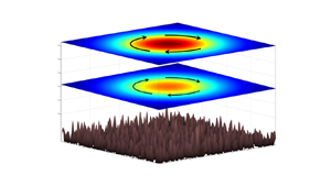
The present model extends the multiscale theory of Radko (Reference Radko2022) to baroclinic flows, layered and continuously stratified. We develop an explicit closure for the topographically induced eddy stresses and validate it by comparing topography-resolving simulations with their parametric counterparts. The sandpaper theory is used to investigate the spin-down of large-scale baroclinic vortices (figure 1). We discover that the influence of topography on such structures is twofold. Topography-induced stresses adversely affect the circulation in regions close to the seafloor. As a result, large-scale flows eventually become equivalent-barotropic, with swift currents constrained to the upper regions and the abyssal zone becoming largely quiescent – patterns that are representative of coherent oceanic eddies (Olson Reference Olson1991). It is also shown that topography stabilizes vortices by suppressing baroclinic instability. This form of instability is caused by the interaction of perturbations at different levels (Phillips Reference Phillips1951) and, therefore, the topographic arrest of abyssal motions dramatically reduces its intensity. We hypothesize that topographic stabilization, illustrated by the sandpaper model, contributes to the surprising sensitivity of oceanic flows to seafloor roughness (LaCasce et al. Reference LaCasce, Escartin, Chassignet and Xu2019; Radko Reference Radko2020; Gulliver & Radko Reference Gulliver and Radko2022).

Figure 1. Schematic diagram illustrating the set-up of the stratified sandpaper model. A large-scale vortex is spinning above the irregular seafloor and its intensity varies with depth.
The paper is organized as follows. Section 2 presents the set-up and governing equations. The multiscale theory for layered flows is developed in § 3 and the resulting parameterization is used to investigate the spin-down and stability of large-scale vortices (§ 4). Section 5 describes the continuously stratified version of the sandpaper model. The results are summarized, and conclusions are drawn, in § 6.
2. Formulation: the layered model
The interaction of large-scale flows with topography is studied using the multilayer framework, which is commonly referred to in the oceanographic literature as the isopycnal model. In the quasi-geostrophic approximation (e.g. Pedlosky Reference Pedlosky1987), the governing equations are
 \begin{align}\left.
{\begin{array}{@{}ll} {\dfrac{{\partial q_1^\ast
}}{{\partial {t^\ast }}} + J(\psi_1^\ast ,q_1^\ast ) +
{\beta^\ast }\dfrac{{\partial \psi_1^\ast }}{{\partial
{x^\ast }}} = {\nu^\ast }{\nabla^4}\psi_1^\ast
,}&{q_1^\ast = {\nabla^2}\psi_1^\ast + \dfrac{{f{{_0^\ast
}^2}}}{{{{g^{\prime}}^\ast }H_1^\ast }}(\psi_2^\ast -
\psi_1^\ast ),}\\ {\dfrac{{\partial q_i^\ast }}{{\partial
{t^\ast }}} + J(\psi_i^\ast ,q_i^\ast ) + {\beta^\ast
}\dfrac{{\partial \psi_i^\ast }}{{\partial {x^\ast }}} =
{\nu^\ast }{\nabla^4}\psi_i^\ast ,\quad i = 2, \ldots ,(n -
1),}&{q_i^\ast = {\nabla^2}\psi_i^\ast +
\dfrac{{f{{_0^\ast }^2}}}{{{{g^{\prime}}^\ast }H_i^\ast
}}(\psi_{i - 1}^\ast + \psi_{i + 1}^\ast - 2\psi_i^\ast
),}\\ {\dfrac{{\partial q_n^\ast }}{{\partial {t^\ast }}} +
J(\psi_n^\ast ,q_n^\ast ) + {\beta^\ast }\dfrac{{\partial
\psi_n^\ast }}{{\partial {x^\ast }}} = {\nu^\ast
}{\nabla^4}\psi_n^\ast - {\gamma^\ast
}{\nabla^2}\psi_n^\ast ,}&{q_n^\ast =
{\nabla^2}\psi_n^\ast + \dfrac{{f{{_0^\ast
}^2}}}{{{{g^{\prime}}^\ast }H_n^\ast }}(\psi_{n -
1}^\ast - \psi_n^\ast ) + f_0^\ast \dfrac{{{\eta^\ast
}}}{{H_n^\ast }},} \end{array}}
\right\}\end{align}
\begin{align}\left.
{\begin{array}{@{}ll} {\dfrac{{\partial q_1^\ast
}}{{\partial {t^\ast }}} + J(\psi_1^\ast ,q_1^\ast ) +
{\beta^\ast }\dfrac{{\partial \psi_1^\ast }}{{\partial
{x^\ast }}} = {\nu^\ast }{\nabla^4}\psi_1^\ast
,}&{q_1^\ast = {\nabla^2}\psi_1^\ast + \dfrac{{f{{_0^\ast
}^2}}}{{{{g^{\prime}}^\ast }H_1^\ast }}(\psi_2^\ast -
\psi_1^\ast ),}\\ {\dfrac{{\partial q_i^\ast }}{{\partial
{t^\ast }}} + J(\psi_i^\ast ,q_i^\ast ) + {\beta^\ast
}\dfrac{{\partial \psi_i^\ast }}{{\partial {x^\ast }}} =
{\nu^\ast }{\nabla^4}\psi_i^\ast ,\quad i = 2, \ldots ,(n -
1),}&{q_i^\ast = {\nabla^2}\psi_i^\ast +
\dfrac{{f{{_0^\ast }^2}}}{{{{g^{\prime}}^\ast }H_i^\ast
}}(\psi_{i - 1}^\ast + \psi_{i + 1}^\ast - 2\psi_i^\ast
),}\\ {\dfrac{{\partial q_n^\ast }}{{\partial {t^\ast }}} +
J(\psi_n^\ast ,q_n^\ast ) + {\beta^\ast }\dfrac{{\partial
\psi_n^\ast }}{{\partial {x^\ast }}} = {\nu^\ast
}{\nabla^4}\psi_n^\ast - {\gamma^\ast
}{\nabla^2}\psi_n^\ast ,}&{q_n^\ast =
{\nabla^2}\psi_n^\ast + \dfrac{{f{{_0^\ast
}^2}}}{{{{g^{\prime}}^\ast }H_n^\ast }}(\psi_{n -
1}^\ast - \psi_n^\ast ) + f_0^\ast \dfrac{{{\eta^\ast
}}}{{H_n^\ast }},} \end{array}}
\right\}\end{align}
where  $\psi _i^\ast $ is the streamfunction in layer i associated with the velocity field
  $(u_i^\ast ,v_i^\ast ) = ( - \partial \psi _i^\ast{/}\partial {y^\ast },\partial \psi _i^\ast{/}\partial {x^\ast })$,
  $H_i^\ast $ is the reference layer thickness,
  ${\eta ^\ast }$ is the topographic height and J is the Jacobian. The asterisks represent dimensional quantities. The lateral viscosity is denoted by
  ${\nu ^\ast }$ and
  ${\gamma ^\ast } = (1/H_n^\ast )\sqrt {\nu _E^\ast f_0^\ast{/}2} $ is the Ekman drag coefficient, where
  $\nu _E^\ast $ is the vertical eddy viscosity in the bottom boundary layer. In the context of the mesoscale spin-down problem,
  ${\nu ^\ast }$ and
  ${\gamma ^\ast }$ represent dissipation induced by small-scale turbulent mixing, rather than molecular friction. Theoretical development is simplified by assuming identical density differences between adjacent layers
  $\Delta {\rho ^\ast } = \rho _i^\ast - \rho _{i - 1}^\ast \,,$ although the generalization to variable
  $\Delta {\rho ^\ast }$ is straightforward. The reduced gravity in (2.1) is denoted by
  ${g^{\prime\ast}} = {g^\ast }(\Delta {\rho ^\ast }/\rho _0^\ast )$, where
  ${g^\ast } \approx 9.8\;\textrm{m}\;{\textrm{s}^{ - 2}}$, and
  ${\beta ^\ast } \equiv \partial {f^\ast }/\partial {y^\ast }$ is the meridional gradient of planetary vorticity. Parameters
  $H_0^\ast $,
  $\rho _0^\ast $ and
  $f_0^\ast $ are the reference values of the ocean depth, density and Coriolis parameter, respectively.
This study explores the interaction of large-scale flow patterns of the lateral extent  $O({L^\ast })$ with much smaller scales
  $O(L_S^\ast )$ that are present in topography. We assume that these small scales are limited to a finite interval
 \begin{equation}L_{min}^\ast < L_S^\ast < L_C^\ast .\end{equation}
The range of small scales is constrained from below to ensure that the Rossby numbers are uniformly low:
 \begin{equation}Ro = \mathop {\max }\limits_{x,y,t,i} \left( {\frac{{|{{\nabla^2}\psi_i^\ast } |}}{{f_0^\ast }}} \right) \ll 1,\end{equation}
as demanded by the quasi-geostrophic approximation. The representative large-scale velocity in the upper (usually most active) layer is denoted by  ${U^\ast }$, and the number of controlling parameters is reduced by non-dimensionalizing
  $\psi _i^\ast $,
  ${x^\ast }$,
  ${y^\ast }$ and
  ${t^\ast }$ as follows:
 \begin{equation}\psi _i^\ast = {U^\ast }{L^\ast }{\psi _i},\quad {x^\ast } = {L^\ast }x,\quad {y^\ast } = {L^\ast }y,\quad {t^\ast } = \frac{{{L^\ast }}}{{{U^\ast }}}t.\end{equation}
For convenience, the depth variation is non-dimensionalized in a different manner:
 \begin{equation}{\eta ^\ast } = \frac{{{U^\ast }H_n^\ast }}{{f_0^\ast {L^\ast }}}\eta .\end{equation}
To be specific, we consider scales that reflect typical sizes and intensities of oceanic mesoscale eddies:
 \begin{equation}{U^\ast } = 0.1\;\textrm{m}\;{\textrm{s}^{ - 1}},\quad {L^\ast } = {10^5}\;\textrm{m},\quad H_0^\ast = 4000\;\textrm{m},\quad f_0^\ast = {10^{ - 4}}\;\textrm{s}{}^{ - 1}.\end{equation}
The non-dimensionalization in (2.4) and (2.5) reduces the governing equations (2.1) to
 \begin{align}\left.
{\begin{array}{@{}ll} {\dfrac{{\partial
{q_1}}}{{\partial t}} + J({\psi_1},{q_1}) + \beta
\dfrac{{\partial {\psi_1}}}{{\partial x}} = \nu
{\nabla^4}{\psi_1},}&{{q_1} = {\nabla^2}{\psi_1} +
{F_1}({\psi_2} - {\psi_1}),}\\ {\dfrac{{\partial
{q_i}}}{{\partial t}} + J({\psi_i},{q_i}) + \beta
\dfrac{{\partial {\psi_i}}}{{\partial x}} = \nu
{\nabla^4}{\psi_i},\quad i = 2, \ldots ,(n - 1),}&{{q_i} =
{\nabla^2}{\psi_i} + {F_i}({\psi_{i - 1}} + {\psi_{i + 1}}
- 2{\psi_i}),}\\ {\dfrac{{\partial {q_n}}}{{\partial t}} +
J({\psi_n},{q_n}) + \beta \dfrac{{\partial
{\psi_n}}}{{\partial x}} = \nu {\nabla^4}{\psi_n} - \gamma
{\nabla^2}{\psi_n},}&{{q_n} = {\nabla^2}{\psi_n} +
{F_n}({\psi_{n - 1}} - {\psi_n}) + \eta ,} \end{array}}
\right\}\end{align}
\begin{align}\left.
{\begin{array}{@{}ll} {\dfrac{{\partial
{q_1}}}{{\partial t}} + J({\psi_1},{q_1}) + \beta
\dfrac{{\partial {\psi_1}}}{{\partial x}} = \nu
{\nabla^4}{\psi_1},}&{{q_1} = {\nabla^2}{\psi_1} +
{F_1}({\psi_2} - {\psi_1}),}\\ {\dfrac{{\partial
{q_i}}}{{\partial t}} + J({\psi_i},{q_i}) + \beta
\dfrac{{\partial {\psi_i}}}{{\partial x}} = \nu
{\nabla^4}{\psi_i},\quad i = 2, \ldots ,(n - 1),}&{{q_i} =
{\nabla^2}{\psi_i} + {F_i}({\psi_{i - 1}} + {\psi_{i + 1}}
- 2{\psi_i}),}\\ {\dfrac{{\partial {q_n}}}{{\partial t}} +
J({\psi_n},{q_n}) + \beta \dfrac{{\partial
{\psi_n}}}{{\partial x}} = \nu {\nabla^4}{\psi_n} - \gamma
{\nabla^2}{\psi_n},}&{{q_n} = {\nabla^2}{\psi_n} +
{F_n}({\psi_{n - 1}} - {\psi_n}) + \eta ,} \end{array}}
\right\}\end{align}
where
 \begin{equation}{F_i} = \frac{{{L^{{\ast} 2}}f{{_0^\ast }^2}}}{{{{g^{\prime}}^\ast }H_i^\ast }},\quad \beta = \frac{{{L^\ast }^2}}{{{U^\ast }}}{\beta ^\ast },\quad \nu = \frac{{{\nu ^\ast }}}{{{U^\ast }{L^\ast }}},\quad \gamma = \frac{{{L^\ast }}}{{{U^\ast }}}{\gamma ^\ast }.\end{equation}
To explore the interaction between flow components of large and small lateral extent, we introduce the scale-separation parameter
 \begin{equation}\varepsilon = \frac{{L_C^\ast }}{{{L^\ast }}} \ll 1.\end{equation}
This parameter is used to define the new set of spatial and temporal scales  $({x_S},{y_S})$ that describe the dynamics of small-scale processes. These variables are related to the original ones through
 \begin{equation}({x_S},{y_S}) = {\varepsilon ^{ - 1}}(x,y),\end{equation}
and the spatial derivatives in the governing system (2.7) are replaced accordingly:
 \begin{equation}\frac{\partial }{{\partial x}} \to \frac{\partial }{{\partial x}} + {\varepsilon ^{ - 1}}\frac{\partial }{{\partial {x_S}}},\quad \frac{\partial }{{\partial y}} \to \frac{\partial }{{\partial y}} + {\varepsilon ^{ - 1}}\frac{\partial }{{\partial {y_S}}}.\end{equation}
We assume that  ${F_i}$,
  $\beta $ and
  $\gamma $ are O(1) quantities, whilst the lateral viscosity (
 $\nu $) is small and therefore rescaled in terms of
  $\varepsilon $:
 \begin{equation}\nu = {\varepsilon ^2}{\nu _0}.\end{equation}
Equation (2.12) implies that friction could be significant on small scales but its direct impact on the large-scale dynamics is weak.
Topographic patterns considered in the following model vary on both large and small scales:
 \begin{equation}\eta = {\eta _L}(x,y) + {\eta _S}({x_S},{y_S}).\end{equation}
The most natural way to separate bathymetry into small-scale and large-scale components – and the one used in our numerical simulations – is based on the Fourier transform:
 \begin{align}
\eta & =\underbrace{{\dfrac{1}{{\sqrt {\Delta k\Delta
l} }}\iint_{\kappa < 2{\rm \pi} /{L_C}} {\tilde{\eta
}(k,l)\,\textrm{exp}(\textrm{i}kx +
{\rm i}ly)\,\textrm{d}k\,\textrm{d}l} }}_{{{\eta _L}}}\nonumber\\ & \quad+
\underbrace{{\dfrac{1}{{\sqrt {\Delta k\Delta l}
}}\iint_{\kappa > 2{\rm \pi} /{L_C}} {\tilde{\eta
}(k,l)\,\textrm{exp}(\textrm{i}kx +
\textrm{i}ly)\,\textrm{d}k\,\textrm{d}l} }}_{{{\eta _S}}},
\end{align}
\begin{align}
\eta & =\underbrace{{\dfrac{1}{{\sqrt {\Delta k\Delta
l} }}\iint_{\kappa < 2{\rm \pi} /{L_C}} {\tilde{\eta
}(k,l)\,\textrm{exp}(\textrm{i}kx +
{\rm i}ly)\,\textrm{d}k\,\textrm{d}l} }}_{{{\eta _L}}}\nonumber\\ & \quad+
\underbrace{{\dfrac{1}{{\sqrt {\Delta k\Delta l}
}}\iint_{\kappa > 2{\rm \pi} /{L_C}} {\tilde{\eta
}(k,l)\,\textrm{exp}(\textrm{i}kx +
\textrm{i}ly)\,\textrm{d}k\,\textrm{d}l} }}_{{{\eta _S}}},
\end{align}
where  $(k,l)$ are the wavenumbers in x and y, tildes denote Fourier images,
  $\kappa \equiv \sqrt {{k^2} + {l^2}} $,
  $(\Delta k,\Delta l) = (2{\rm \pi} L_x^{ - 1},2{\rm \pi} L_y^{ - 1})$ and
  $({L_x},{L_y})$ is the domain size. The component
  ${\eta _L}$ of decomposition (2.14) gently varies on relatively large scales and
  ${\eta _S}$ represents small-scale variability.
For representative magnitudes of depth variation  ${\eta ^\ast }\sim 300\;\textrm{m}$ (Goff & Jordan Reference Goff and Jordan1988; Goff Reference Goff2020), their non-dimensional counterparts significantly exceed unity:
  $\eta \sim 10$. This variability is mostly associated with relatively small lateral scales (~10 km). Therefore, the small-scale depth variation is rescaled as
 \begin{equation}{\eta _S} = {\varepsilon ^{ - 1}}{\eta _0}. \end{equation}
3. Multiscale model
We now proceed to develop a baroclinic version of the sandpaper theory. Our approach is analogous to the barotropic model of Radko (Reference Radko2022) and only an abbreviated description is offered here. To capture the interaction of large-scale patterns with small-scale topography, the solution for  ${\psi _i}$ is sought in terms of power series in
  $\varepsilon \ll 1$:
 \begin{equation}{\psi _i} = \psi _i^{(0)}(x,y,t) + \varepsilon \psi _i^{(1)}(x,y,{x_S},{y_S},t) + {\varepsilon ^2}\psi _i^{(2)}(x,y,{x_S},{y_S},t) + \cdots .\end{equation}
 The expansion opens with a large-scale pattern  $\psi _i^{(0)}$ that does not vary on small scales. We modify the governing equations (2.7) using (2.11)–(2.15) and substitute series (3.1) in the resulting expressions, combining terms of the same order in
  $\varepsilon $. The leading-order
  $O({\varepsilon ^{ - 2}})$ balance in all layers except for the bottom one is trivially solved by
 \begin{equation}\psi _i^{(1)} = 0,\quad i = 1, \ldots ,(n - 1),\end{equation}
whereas for the lowest layer we use the steady small-scale pattern  $\psi _n^{(1)} = \psi _n^{(1)}({x_S},{y_S})$ that satisfies
 \begin{equation}\nabla _S^2\psi _n^{(1)} + {\eta _0}({x_S},{y_S}) = 0,\end{equation}
where  $\nabla _S^2 \equiv {\partial ^2}/\partial x_S^2 + {\partial ^2}/\partial y_S^2$. This balance represents the tendency for expulsion of small-scale potential vorticity (PV) in the lowest layer (Radko Reference Radko2022).
The  $O({\varepsilon ^{ - 1}})$ balances in the upper layers are satisfied by
 \begin{equation}\psi _i^{(2)} = 0,\quad i = 1, \ldots ,(n - 1),\end{equation}
and the corresponding balance for the bottom layer amounts to
 \begin{equation}\left( {\frac{{\partial \psi_n^{(0)}}}{{\partial x}} + \frac{{\partial \psi_n^{(1)}}}{{\partial {x_S}}}} \right)\frac{{\partial \varsigma _n^{(2)}}}{{\partial {y_S}}} - \left( {\frac{{\partial \psi_n^{(0)}}}{{\partial y}} + \frac{{\partial \psi_n^{(1)}}}{{\partial {y_S}}}} \right)\frac{{\partial \varsigma _n^{(2)}}}{{\partial {x_S}}} = {\nu _0}\nabla _S^4\psi _n^{(1)} - \gamma \nabla _S^2\psi _n^{(1)},\end{equation}
where  $\varsigma _n^{(2)} \equiv \nabla _S^2\psi _n^{(2)}$. The physical interpretation of (3.5) is straightforward. The advection of the small-scale PV field – represented by
  $\varsigma _n^{(2)}$ at the leading order – by the primary large-scale flow is balanced by explicit dissipation. While
  $\psi _n^{(1)}$ is rigidly controlled by topography and therefore is steady, the second-order correction
  $\psi _n^{(2)}$ is time-dependent and sensitive to the changes in the large-scale flow (
 $\psi _n^{(0)}$). It is also interesting to note that while the lateral friction (
 $\nu $) is weak and does not affect the large-scale flow directly, its indirect influence can be substantial. Friction affects the small-scale pattern through the advective–diffusive balance (3.5). The small-scale eddies, in turn, can influence large-scale flows by generating substantial Reynolds stresses.
The evolutionary equations are obtained from the  $O(1)$ balances by averaging them in small-scale variables, which yields
 \begin{align}\left.
{\begin{array}{@{}ll} {\dfrac{{\partial
q_1^{(0)}}}{{\partial t}} + J(\psi_1^{(0)},q_1^{(0)}) +
\beta \dfrac{{\partial \psi_1^{(0)}}}{{\partial x}} =
0,}&{q_1^{(0)} = {\nabla^2}\psi_1^{(0)} +
{F_1}(\psi_2^{(0)} - \psi_1^{(0)}),}\\ {\dfrac{{\partial
q_i^{(0)}}}{{\partial t}} + J(\psi_i^{(0)},q_i^{(0)}) +
\beta \dfrac{{\partial \psi_i^{(0)}}}{{\partial x}} =
0,\quad i = 2, \ldots ,(n - 1),}&{q_i^{(0)} =
{\nabla^2}\psi_i^{(0)} + {F_i}(\psi_{i - 1}^{(0)} + \psi_{i
+ 1}^{(0)} - 2\psi_i^{(0)}),}\\ {\dfrac{{\partial
q_n^{(0)}}}{{\partial t}} + J(\psi_n^{(0)},q_n^{(0)}) +
\beta \dfrac{{\partial \psi_n^{(0)}}}{{\partial x}} + D +
\gamma {\nabla^2}\psi_n^{(0)} = 0,}&{q_n^{(0)} =
{\nabla^2}\psi_n^{(0)} + {F_n}(\psi_{n - 1}^{(0)} -
\psi_n^{(0)}) + {\eta_L},} \end{array}}
\right\}\end{align}
\begin{align}\left.
{\begin{array}{@{}ll} {\dfrac{{\partial
q_1^{(0)}}}{{\partial t}} + J(\psi_1^{(0)},q_1^{(0)}) +
\beta \dfrac{{\partial \psi_1^{(0)}}}{{\partial x}} =
0,}&{q_1^{(0)} = {\nabla^2}\psi_1^{(0)} +
{F_1}(\psi_2^{(0)} - \psi_1^{(0)}),}\\ {\dfrac{{\partial
q_i^{(0)}}}{{\partial t}} + J(\psi_i^{(0)},q_i^{(0)}) +
\beta \dfrac{{\partial \psi_i^{(0)}}}{{\partial x}} =
0,\quad i = 2, \ldots ,(n - 1),}&{q_i^{(0)} =
{\nabla^2}\psi_i^{(0)} + {F_i}(\psi_{i - 1}^{(0)} + \psi_{i
+ 1}^{(0)} - 2\psi_i^{(0)}),}\\ {\dfrac{{\partial
q_n^{(0)}}}{{\partial t}} + J(\psi_n^{(0)},q_n^{(0)}) +
\beta \dfrac{{\partial \psi_n^{(0)}}}{{\partial x}} + D +
\gamma {\nabla^2}\psi_n^{(0)} = 0,}&{q_n^{(0)} =
{\nabla^2}\psi_n^{(0)} + {F_n}(\psi_{n - 1}^{(0)} -
\psi_n^{(0)}) + {\eta_L},} \end{array}}
\right\}\end{align}
where
 \begin{equation}D = {\left\langle {\frac{{\partial \psi_n^{(1)}}}{{\partial {x_S}}}\frac{{\partial \varsigma_n^{(2)}}}{{\partial y}} - \frac{{\partial \psi_n^{(1)}}}{{\partial {y_S}}}\frac{{\partial \varsigma_n^{(2)}}}{{\partial x}}} \right\rangle _{{x_S},{y_S}}}.\end{equation}
Angle brackets represent mean values, with the averaging variables listed in the subscript.
In (3.6), we readily recognize the original governing equations that are modified in two ways. They no longer contain explicit lateral friction, which is not surprising since viscosity is treated as a weak higher-order correction. More significant, however, is the appearance of term D in the equation for the bottom layer, which represents the topographic forcing of large-scale flows by small-scale bottom roughness. It should be emphasized that topographic forcing ( $D$) originates from the averaged nonlinear advective term
  $J({\psi ^{\prime}_n},{\nabla ^2}{\psi ^{\prime}_n})$ in (2.7), where
  ${\psi ^{\prime}_n} = {\psi _n} - \psi _n^{(0)}$, and represents the eddy-induced mixing of momentum. This finding brings precious insight into the physics of topographic control. It implies that the primary role of topography in the sandpaper model is the generation of small-scale eddies that affect large-scale flows through the associated Reynolds stresses. In contrast, the topographic “form drag” acting directly on the large-scale current, which is represented by term
  $J(\psi _n^{(0)},{\eta _S})$, does not affect the large-scale circulation at the leading order.
At this point, it becomes necessary to express the topographic forcing (3.7) in terms of zero-order flow components. This challenge is met by recognizing that  $\psi _n^{(1)}$ can be computed for any given pattern of small-scale topography using (3.3) and
  $\varsigma _n^{(2)}$ can be obtained from (3.5). The analytical steps used to eliminate
  $\varsigma _n^{(2)}$ between (3.5) and (3.7) are essentially identical to those taken in the barotropic model (Radko Reference Radko2022) but, for convenience, they are reproduced in Appendix A. The result of these developments is the explicit expression for D in terms of large-scale velocities:
 \begin{equation}D = G\left( {\frac{\partial }{{\partial x}}\left( {\frac{{{v_n}}}{{u_n^2 + v_n^2}}} \right) - \frac{\partial }{{\partial y}}\left( {\frac{{{u_n}}}{{u_n^2 + v_n^2}}} \right)} \right)\,,\quad G = 2{\rm \pi} \int {{{|{{{\tilde{\eta }}_S}} |}^2}\left( {\frac{\gamma }{\kappa } + \nu \kappa } \right)\textrm{d}\kappa } ,\end{equation}
where  $(k,l)$ are the wavenumbers,
  $\kappa = \sqrt {{k^2} + {l^2}}$,
  $({u_n},{v_n}) = ( - \partial {\psi _n}/\partial y,\partial {\psi _n}/\partial x)$ and
  ${\tilde{\eta }_S}$ represents the Fourier image of the small-scale component of topography. To lighten up notation, we omit superscripts ‘(0)’ in leading-order flow components since the subsequent discussion is focused exclusively on their dynamics. Note that the coefficient G in the topographic forcing term (3.8) is uniquely determined by the bathymetric spectrum and the explicit dissipation parameters
  $(\gamma ,\nu )$. Therefore, (3.8) can be viewed as a rigorous parameterization of the topographic forcing of large-scale flows. It should be emphasized, however, that the performance of this closure is contingent on the effective homogenization of small-scale PV, as demanded by (3.3). The extent to which the homogenization is realized in nature may be configuration-dependent.
To help in implementing the sandpaper theory in more utilitarian applications, we also include the dimensional expression of the topographic forcing:
 \begin{align}{D^\ast } = {G^\ast }\left( {\frac{\partial }{{\partial {x^\ast }}}\left( {\frac{{v_n^\ast }}{{u_n^{{\ast} 2} + v_n^{{\ast} 2}}}} \right) - \frac{\partial }{{\partial {y^\ast }}}\left( {\frac{{u_n^\ast }}{{u_n^{{\ast} 2} + v_n^{{\ast} 2}}}} \right)} \right),\quad {G^\ast } = \frac{{2{\rm \pi} f_0^{{\ast} 2}}}{{H_n^{{\ast} 2}}}\int {{{|{\tilde{\eta }_S^\ast } |}^2}\left( {\frac{{{\gamma^\ast }}}{{{\kappa^\ast }}} + {\nu^\ast }{\kappa^\ast }} \right)\textrm{d}{\kappa ^\ast }} .\end{align}
The topographic forcing term  ${D^\ast }$ can be introduced in the dimensional quasi-geostrophic equation for the bottom layer (2.1) to represent the effects of unresolved bathymetry. We also note that adding topographic forcing (3.9) in the PV equation is equivalent to modifying the horizontal momentum equations as follows:
 \begin{equation}\left.
{\begin{array}{c@{}} {\dfrac{{\partial u_n^\ast
}}{{\partial {t^\ast }}} + u_n^\ast \dfrac{{\partial
u_n^\ast }}{{\partial {x^\ast }}} + v_n^\ast
\dfrac{{\partial u_n^\ast }}{{\partial {y^\ast }}} -
{f^\ast }v_n^\ast = - \dfrac{1}{{\rho_n^\ast
}}\dfrac{{\partial p_n^\ast }}{{\partial {x^\ast }}} -
\dfrac{{{G^\ast }u_n^\ast }}{{u_n^{{\ast} \,2} +
v_n^{{\ast} \,2}}} + {\nu^\ast }{\nabla^2}u_n^\ast ,}\\
{\dfrac{{\partial v_n^\ast }}{{\partial {t^\ast }}} +
u_n^\ast \dfrac{{\partial v_n^\ast }}{{\partial {x^\ast }}}
+ v_n^\ast \dfrac{{\partial v_n^\ast }}{{\partial {y^\ast
}}} + {f^\ast }u_n^\ast = - \dfrac{1}{{\rho_n^\ast
}}\dfrac{{\partial p_n^\ast }}{{\partial {y^\ast }}} -
\dfrac{{{G^\ast }v_n^\ast }}{{u_n^{{\ast} \,2} +
v_n^{{\ast} \,2}}} + {\nu^\ast }{\nabla^2}v_n^\ast ,}
\end{array}} \right\}\end{equation}
\begin{equation}\left.
{\begin{array}{c@{}} {\dfrac{{\partial u_n^\ast
}}{{\partial {t^\ast }}} + u_n^\ast \dfrac{{\partial
u_n^\ast }}{{\partial {x^\ast }}} + v_n^\ast
\dfrac{{\partial u_n^\ast }}{{\partial {y^\ast }}} -
{f^\ast }v_n^\ast = - \dfrac{1}{{\rho_n^\ast
}}\dfrac{{\partial p_n^\ast }}{{\partial {x^\ast }}} -
\dfrac{{{G^\ast }u_n^\ast }}{{u_n^{{\ast} \,2} +
v_n^{{\ast} \,2}}} + {\nu^\ast }{\nabla^2}u_n^\ast ,}\\
{\dfrac{{\partial v_n^\ast }}{{\partial {t^\ast }}} +
u_n^\ast \dfrac{{\partial v_n^\ast }}{{\partial {x^\ast }}}
+ v_n^\ast \dfrac{{\partial v_n^\ast }}{{\partial {y^\ast
}}} + {f^\ast }u_n^\ast = - \dfrac{1}{{\rho_n^\ast
}}\dfrac{{\partial p_n^\ast }}{{\partial {y^\ast }}} -
\dfrac{{{G^\ast }v_n^\ast }}{{u_n^{{\ast} \,2} +
v_n^{{\ast} \,2}}} + {\nu^\ast }{\nabla^2}v_n^\ast ,}
\end{array}} \right\}\end{equation}
where  $p_n^\ast $ is the pressure field in the bottom layer. Formulation (3.10) permits the implementation of the proposed parameterization in isopycnal general circulation models (e.g. Bleck Reference Bleck2002), commonly used for large-scale ocean simulations.
4. Spin-down of a baroclinic vortex
The objective of the following simulations is twofold. We examine the mechanics of topographic spin-down of circular vortices and concurrently assess the performance characteristics of the parametric model (3.8). The latter goal is achieved by comparing topography-resolving simulations with their parametric counterparts. The configuration of the spin-down experiments is illustrated in figure 1.
The bottom topography is represented by the observationally derived spectrum of Goff & Jordan (Reference Goff and Jordan1988):
 \begin{equation}P_\eta ^\ast = \frac{{h_{}^{{\ast} \,2}(\mu - 2)}}{{{{(2{\rm \pi} )}^3}k_0^\ast l_0^\ast }}{\left( {1 + {{\left( {\frac{{{k^\ast }}}{{2{\rm \pi} k_0^\ast }}} \right)}^2} + {{\left( {\frac{{{l^\ast }}}{{2{\rm \pi} l_0^\ast }}} \right)}^2}} \right)^{ - \mu /2}}.\end{equation}
Following Nikurashin et al. (Reference Nikurashin, Ferrari, Grisouard and Polzin2014), we assume
 \begin{equation}\mu = 3.5,\quad k_0^\ast = 1.8 \times {10^{ - 4}}\;{\textrm{m}^{ - 1}},\quad l_0^\ast = 1.8 \times {10^{ - 4}}\;{\textrm{m}^{ - 1}},\quad {h^\ast } = 305\;\textrm{m}.\end{equation}
After non-dimensionalization, (4.1) reduces to
 \begin{equation}{P_\eta } = C{\left( {1 + {{\left( {\frac{\kappa }{{2{\rm \pi} {L^\ast }k_0^\ast }}} \right)}^2}} \right)^{ - \mu /2}},\quad C = \frac{{\mu - 2}}{{{{(2{\rm \pi} )}^3}}}{\left( {\frac{{f_0^\ast {h^\ast }}}{{{U^\ast }H_n^\ast k_0^\ast }}} \right)^2}.\end{equation}
For topography-resolving simulations, we reconstruct bottom topography as a sum of Fourier modes with random phases and spectral amplitudes conforming to (4.3). The range of small-scale variability (2.2) is specified by assigning  ${L_{min}} = 0.03$ and
  ${L_C} = 0.3\,,$which is dimensionally equivalent to
  $L_{min}^\ast = 3\;\textrm{km}$ and
  $L_C^\ast = 30\;\textrm{km}$. The components of topography with wavelengths outside of this interval (
 $2{\rm \pi} {\kappa ^{ - 1}} > {L_C}$ and
  $2{\rm \pi} {\kappa ^{ - 1}} < {L_{min}}$) are excluded from the bathymetric spectrum.
All experiments, parametric and topography-resolving, are performed with the two-layer  $(n = 2)$ model. The simulations are initiated with the Gaussian streamfunctions for both layers:
 \begin{equation}\left. \begin{array}{@{}l} \psi_1^G = {\rm exp} ( - {r^2})\\ \psi_2^G = A\,\textrm{exp}( - {r^2}) \end{array} \quad r = \sqrt {{x^2} + {y^2}}. \right\}\end{equation}
Without loss of generality, the effective non-dimensional radius and the amplitude of the upper layer flow are set to unity. The second-layer amplitude  $(A)$ determines the initial baroclinicity of the vortex (4.4). The governing equations are integrated using the de-aliased pseudo-spectral model employed in our previous works (e.g. Radko & Kamenkovich Reference Radko and Kamenkovich2017; Radko, McWilliams & Sutyrin Reference Radko, McWilliams and Sutyrin2022). A relatively wide computational domain of size
  $({L_x},{L_y}) = (8,8)$ is used to limit the influence of boundary conditions. The topography-resolving simulations employ a fine mesh with
  $({N_x},{N_y}) = (2048,2048)$ grid points. The parametric simulations, which do not require the resolution of small-scale bathymetry, are performed on a much coarser grid with
  $({N_x},{N_y}) = (256,256)$. For our baseline configuration, we assume
  ${F_1} = 10$ and
  ${F_2} = {\textstyle{{10} \over 3}},$ which corresponds to
  ${g^{\prime\ast}} = 0.01\;\textrm{m}\,{\textrm{s}^{ - 1}}$,
  $H_1^\ast = 1\;\textrm{km}$ and
  $H_2^\ast = 3\;\textrm{km}$. The lateral viscosity is
  $\nu = {10^{ - 4}}$ and
  $\gamma = \beta = 0$.
While topography-resolving simulations are readily performed using (2.7), numerical treatments of the parametric system demand the modification of (3.6). One of the complications is caused by the singularity of the topographic forcing term (3.8) in locations where the absolute velocity in the bottom layer  $V = \sqrt {u_n^2 + v_n^2} $ is zero. Following Radko (Reference Radko2022), this problem is mitigated by introducing the modified velocity
 \begin{equation}{V_m} = \frac{V}{{{{\tanh }^2}(\delta V)}},\end{equation}
where  $\delta \gg 1$. In all simulations reported here, we use
  $\delta = 25$. While
  ${V_m} \approx V$ for most of the vortex area, (4.5) guarantees that the modified velocity is non-zero at any given point. The expression for D is adjusted accordingly:
 \begin{equation}{D_m} = G\left( {\frac{\partial }{{\partial x}}\left( {\frac{{{v_n}}}{{V{V_m}}}} \right) - \frac{\partial }{{\partial y}}\left( {\frac{{{u_n}}}{{V{V_m}}}} \right)} \right).\end{equation}
Another technical complication is caused by the lack of explicit lateral dissipation in (3.6), which is scaled as  $O({\varepsilon ^2})$ in the asymptotic theory. Since lateral viscosity is required to control the numerical stability of nonlinear simulations, it is reintroduced in the parametric model as follows:
 \begin{align}\left.
{\begin{array}{@{}ll} {\dfrac{{\partial
{q_1}}}{{\partial t}} + J({\psi_1},{q_1}) + \beta
\dfrac{{\partial {\psi_1}}}{{\partial x}} = \nu
{\nabla^4}{\psi_1},}&{{q_1} = {\nabla^2}{\psi_1} +
{F_1}({\psi_2} - {\psi_1}),}\\ {\dfrac{{\partial
{q_i}}}{{\partial t}} + J({\psi_i},{q_i}) + \beta
\dfrac{{\partial {\psi_i}}}{{\partial x}} = \nu
{\nabla^4}{\psi_i},\quad i = 2, \ldots (n - 1),}&{{q_i} =
{\nabla^2}{\psi_i} + {F_i}({\psi_{i - 1}} + {\psi_{i + 1}}
- 2{\psi_i}),}\\ {\dfrac{{\partial {q_n}}}{{\partial t}} +
J({\psi_n},{q_n}) + \beta \dfrac{{\partial
{\psi_n}}}{{\partial x}} + {D_m} + \gamma
{\nabla^2}{\psi_n} = \nu {\nabla^4}{\psi_n},}&{{q_n} =
{\nabla^2}{\psi_n} + {F_n}({\psi_{n - 1}} - {\psi_n}) +
{\eta_L}.} \end{array}}
\right\}\end{align}
\begin{align}\left.
{\begin{array}{@{}ll} {\dfrac{{\partial
{q_1}}}{{\partial t}} + J({\psi_1},{q_1}) + \beta
\dfrac{{\partial {\psi_1}}}{{\partial x}} = \nu
{\nabla^4}{\psi_1},}&{{q_1} = {\nabla^2}{\psi_1} +
{F_1}({\psi_2} - {\psi_1}),}\\ {\dfrac{{\partial
{q_i}}}{{\partial t}} + J({\psi_i},{q_i}) + \beta
\dfrac{{\partial {\psi_i}}}{{\partial x}} = \nu
{\nabla^4}{\psi_i},\quad i = 2, \ldots (n - 1),}&{{q_i} =
{\nabla^2}{\psi_i} + {F_i}({\psi_{i - 1}} + {\psi_{i + 1}}
- 2{\psi_i}),}\\ {\dfrac{{\partial {q_n}}}{{\partial t}} +
J({\psi_n},{q_n}) + \beta \dfrac{{\partial
{\psi_n}}}{{\partial x}} + {D_m} + \gamma
{\nabla^2}{\psi_n} = \nu {\nabla^4}{\psi_n},}&{{q_n} =
{\nabla^2}{\psi_n} + {F_n}({\psi_{n - 1}} - {\psi_n}) +
{\eta_L}.} \end{array}}
\right\}\end{align}
Our first comparison of the topography-resolving and parametric models is based on the vortex spin-down experiment performed with  $A = 0.5$ (figure 2). The instantaneous
  $(t = 10)$ streamfunction patterns
  ${\psi _1}$ and
  ${\psi _2}$ in the topography-resolving simulation are shown in figure 2(a,b), and their parametric counterparts in figure 2(c,d). Topography-resolving and parametric simulations are generally consistent with each other. They reveal a major reduction in the streamfunction amplitudes, from (1, 0.5) in the upper and lower layers initially to (0.69, 0.13) in the topography-resolving run and to (0.71, 0.15) in the parametric simulation. Such agreement instils confidence in the ability of the sandpaper model to capture the essential physics of the flow–topography interaction. This belief is reinforced by comparing the lower-layer vorticity and topography in figure 3, which presents a magnified view of a small region in the vortex interior:
 \begin{equation}\varOmega = \{ 0.4 < x < 0.6,\;0.4 < y < 0.6\} .\end{equation}
Figure 2. Streamfunction patterns in the topography-resolving (t-r) experiment at  $t = 10$ in the (a) upper and (b) lower layers. (c,d) The corresponding patterns in parametric simulations (par).

Figure 3. Magnified views of the (a) lower-layer vorticity and (b) depth perturbation in the small area (4.8).
According to (3.3), the vorticity and topographic patterns represent mirror images of each other,  ${\varsigma _2} \approx - {\eta _S}$, and even the visual inspection of figure 3 readily confirms this proposition. For a more quantitative assessment, we compute the correlation coefficient of
  ${\varsigma _2}$ and
  ${\eta _S}$:
 \begin{equation}c = \frac{{{{\langle {\varsigma _2}{\eta _S}\rangle }_\varOmega }}}{{\sqrt {{{\langle \varsigma _2^2\rangle }_\varOmega }{{\langle \eta _S^2\rangle }_\varOmega }} }} = - 0.98.\end{equation}
Such anticorrelation is the spectacular manifestation of the small-scale PV homogenization – the cornerstone of the sandpaper theory.
To further explore the spin-down dynamics, we turn to the temporal record of kinetic energy  ${E_i} = {\textstyle{1 \over 2}}{\langle {|{\boldsymbol{\nabla }{\psi_i}} |^2}\rangle _{x,y}}$, where
  $i = 1,2$. Once again, the topography-resolving and parametric simulations (figure 4) are generally in agreement. Qualitative differences in the energy patterns are observed only at the initial stage of the simulation (
 $t < 1$), when
  ${E_1}$ in the topography-resolving experiment decreases much more rapidly than its parametric counterpart. Afterwards (
 $t > 1$), the spin-down rates become much closer. The transient initial response reflects the adjustment of the flow field in the topography-resolving simulation to the balanced state characterized by the small-scale PV homogenization. Particularly telling in this regard is the record of the correlation coefficient (4.9), which changes over the adjustment period
  $0 < t < 1$ from
  $c = - 0.03$ to
  $c = - 0.92$. While the energy substantially decreases in both layers, the spin-down of the lower one is more dramatic. By
  $t = 20$, the system transitions to a nearly steady equivalent-barotropic state in which the abyssal region is effectively quiescent and circulation is limited to the upper layer. For reference, figure 4 also includes the energy record from the corresponding flat-bottom experiment. The vortex barely changes throughout this simulation
  $(0 < t < 30)$, and its upper (lower) layer energy reduces by less than 2 % (3 %).

Figure 4. Time series of mean kinetic energy in the upper (a) and lower (b) layers for the experiment with  $A = 0.5$. The topography-resolving, parametric and flat-bottom simulations are indicated by solid, dashed and dotted curves, respectively.
In the next example, we reverse the sense of rotation in the lower layer by assigning  $A = - 0.5$. The time series of energy in this case (figure 5) reveal a considerably different evolutionary pattern (cf. figure 4). While the abyssal flow still rapidly slows down, the upper layer accelerates, almost doubling its energy. This spin-up is attributed to the release of the potential energy associated with the sloping interface between the upper and lower layers. As the abyssal circulation weakens, the interface flattens due to the Margules effect (von Helmholtz Reference von Helmholtz1888; Margules Reference Margules1906). The associated reduction of the available potential energy of the system prompts its partial transfer into the kinetic energy of the upper layer. However, by
  $t \approx 20$, the system evolves to an equivalent-barotropic state. As in the previous example (figure 4), the topography-resolving and parametric simulations are generally consistent. The only significant differences in the corresponding energy patterns occur during the brief initial adjustment period
  $(t < 1)$.

Figure 5. Same as in figure 4, but for the experiment with  $A = - 0.5$.
An interesting aspect of the evolution of a vortex with counter-rotating circulations at different levels is its stability. In such structures, the sign of radial PV gradients changes with depth, and therefore these vortices meet the linear instability criterion (Dritschel Reference Dritschel1988). To further explore this issue, the topography-resolving and flat-bottom simulations in figure 5 were extended in time to  $t = 100$. The results (figure 6) reveal the profound influence of the seafloor roughness on vortex stability. The vortex in the flat-bottom experiment gradually loses its axial symmetry and eventually splits into two smaller eddies. In contrast, the vortex above irregular topography remains coherent and nearly steady throughout the entire simulation. This topographic stabilization is consistent with our earlier findings (Gulliver & Radko Reference Gulliver and Radko2022) and calls for a more systematic analysis.

Figure 6. Snapshots of  ${\psi _1}$ at (a,b) t = 70, (c,d) t = 75 and (e, f) t = 80 in the topography-resolving (a,c,e) and flat-bottom ( f-b) (b,d, f) simulations.
To this end, we take advantage of the dramatic reduction in the computational cost of simulations brought by the parametric model, which makes it feasible to explore the relevant parameter space in detail. Of particular interest is the analysis of the maximal growth rate of unstable perturbations ( $\lambda $). This quantity is computed by linearizing the parametric equations (4.7) with respect to the basic state (4.4). Since all simulations with irregular seafloor are characterized by the suppression of the abyssal circulation (figures 4 and 5), we focus on the equivalent-barotropic vortices with
  $A = 0$. The linearized equations are integrated in time, starting from the random distribution of perturbations
  $({\varphi _1},{\varphi _2}) = ({\psi _1} - \psi _1^G,{\psi _2})$. We employ the spectral algorithm analogous to the one used for the nonlinear simulations. Since linearized simulations do not require explicit dissipation, the lateral friction terms (
 $\nu {\nabla ^2}{\psi _i}$) are not included. The linear system eventually becomes dominated by the most rapidly amplifying mode, which makes it possible to determine the maximal growth rate.
The procedure used to compute  $\lambda $ is illustrated in figure 7. Figure 7(a) presents the temporal records of
  ${\textstyle{1 \over 2}}\,\textrm{ln}({E^{\prime}_1})$, where
  ${E^{\prime}_1}(t) = {\textstyle{1 \over 2}}{|{\boldsymbol{\nabla }{\varphi_1}} |^2}$ is the perturbation energy in the upper layer. As previously, we assume
  ${F_1} = 10$ and
  ${F_2} = {\textstyle{{10} \over 3}}$. The calculations were performed for various values of the coefficient G in the topographic forcing term (4.6), a subset of which is shown in figure 7(a). In each case, after a brief period of adjustment, the perturbation starts growing/decaying exponentially. The maximal growth rates are evaluated from the best linear fit to
  ${\textstyle{1 \over 2}}\,\textrm{ln}({E_1})$ over the second half of each simulation
  $(250 < t < 500)$ and plotted as a function of G in figure 7(b). These diagnostics reveal that the growth rates rapidly decrease with increasing G. For sufficiently high values of G, the vortex becomes linearly stable.

Figure 7. (a) Temporal records of  ${\textstyle{1 \over 2}}\,\textrm{ln}({E^{\prime}_1})$ for various values of G. The maximal growth rates are determined from the best linear fits to these records over the second half of the integration interval. (b) Growth rates obtained in this manner are plotted as a function of G.
To offer a more systematic analysis of the growth rates and their dependencies on governing parameters, we independently vary G and  ${F_1}$ (the inverse Burger number), whilst maintaining the original layer depth ratio of
  $R = {H_2}/{H_1} = {F_1}/{F_2} = 3$. The resulting growth rate pattern
  $\lambda ({F_1},G)$ in figure 8(a) reveals higher susceptibility of relatively large-scale (high-
 ${F_1}$) vortices to baroclinic instability. In figure 8(b), we assume
  ${F_1} = 10$ and examine the dependence of growth rates on G and R. As expected,
  $\lambda $ decreases with increasing R, which implies that relatively shallow vortices that are confined to subsurface regions tend to be more stable than their deeper counterparts.

Figure 8. Growth rate ( $\lambda $) is plotted as (a) a function of G and
  ${F_1}$ and (b) a function of G and R.
However, the most significant revelation in figure 8 is the remarkable sensitivity of vortices to even the smallest values of topographic forcing. For  $G > {G_{cr}} \approx {10^{ - 3}}$, the Gaussian upper-layer vortex becomes stable for all relevant values of
  ${F_1}$ and
  ${F_2}$. For a representative topography spectrum (4.2), this critical value (
 ${G_{cr}}$) can be achieved either with
  ${\nu _{cr}} = 1.5 \times 10{}^{ - 5}$ (
 $\nu _{cr}^\ast = 0.15\;{\textrm{m}^2}\;{\textrm{s}^{ - 1}}$) or with
  ${\gamma _{cr}} = 0.065$
  $(\gamma _{cr}^\ast = 6.5 \times {10^{ - 8}}\;{\textrm{s}^{ - 1}})$. Note that the explicit dissipation coefficients in this study represent eddy-induced (rather than molecular) processes. Although the estimates of submesoscale mixing are poorly constrained by observations and models, it is very likely that
  $(\nu ,\gamma )$ in the ocean commonly exceed these instability thresholds
  $({\nu _{cr}},{\gamma _{cr}})$. For instance, the analysis of several observational datasets consolidated by Li et al. (Reference Li, Sun and Xu2018) suggests that the effective lateral viscosities are scale-dependent and can be described (in MKS units) by an empirical relation
  ${\nu ^\ast } = {10^{ - 6}}{a^{1.8}}$, where a is the scale of a phenomenon of interest. For the range of topographic scales considered in this study
  $(3 \times {10^3}\;\textrm{m} < L_S^\ast < 3 \times {10^4}\,\textrm{m})$, this estimate yields
  $1\;{\textrm{m}^2}\;{\textrm{s}^{ - 1}}\begin{array}{*{20}{c}} < \\ \sim \end{array}{\nu ^\ast }\begin{array}{*{20}{c}} < \\ \sim \end{array}100\;{\textrm{m}^2}\;{\textrm{s}^{ - 1}}$ exceeding
  $\nu _{cr}^\ast $ by at least an order of magnitude. The broadly representative Ekman friction coefficient in the oceanic bottom boundary layer is
  ${\gamma ^\ast }\sim {10^{ - 7}}\;{\textrm{s}^{ - 1}}$ (e.g. Arbic & Flierl Reference Arbic and Flierl2004). This value also exceeds the critical threshold (
 $\gamma _{cr}^\ast $) and therefore the Reynolds stresses attributed to the Ekman friction are by themselves sufficient to stabilize coherent vortices. Furthermore, we should keep in mind that the foregoing analysis is based on the quasi-geostrophic model, which a priori excludes internal gravity waves and the associated wave-induced topographic drag. The wave drag can be substantial (e.g. Arbic et al. Reference Arbic, Fringer, Klymak, Mayer, Trossman and Zhu2019) and acts in the same sense as the Reynolds stresses in the sandpaper model, which is expected to stabilize vortices even more. Thus, it appears that bottom roughness may be the answer to the long-standing mystery of the remarkable longevity and stability of the ocean rings (e.g. Dewar & Killworth Reference Dewar and Killworth1995, Reference Dewar and Killworth1999; Dewar et al. 1999).
5. Continuously stratified model
While the foregoing theory and associated simulations were based on a multilayer model, some reflection suggests that they can be generalized for continuously stratified flows. To that end, we consider the continuously stratified quasi-geostrophic framework (e.g. Pedlosky Reference Pedlosky1987):
 \begin{equation}\frac{{\partial {q^\ast }}}{{\partial {t^\ast }}} + J({\psi ^\ast },{q^\ast }) + {\beta ^\ast }\frac{{\partial {\psi ^\ast }}}{{\partial {x^\ast }}} = {\nu ^\ast }{\nabla ^2}{\psi ^\ast },\quad {q^\ast } = {\nabla ^2}{\psi ^\ast } + \frac{\partial }{{\partial {z^\ast }}}\left( {\frac{{f_0^{{\ast} 2}}}{{N{}^{{\ast} 2}}}\frac{{\partial {\psi^\ast }}}{{\partial {z^\ast }}}} \right),\end{equation}
where  ${N^\ast }(z) = \sqrt { - ({g^\ast }/\rho _0^\ast )(\partial {{\bar{\rho }}^\ast }/\partial {z^\ast })} $ is the background pattern of the Brunt–Väisälä frequency. The boundary conditions at the sea surface and bottom are as follows:
 \begin{align}\left.\begin{array}{@{}l}
\dfrac{\partial }{{\partial {t^\ast }}}\left(
{\dfrac{{\partial {\psi^\ast }}}{{\partial {z^\ast }}}}
\right) + J\left( {{\psi^\ast },\dfrac{{\partial {\psi^\ast
}}}{{\partial {z^\ast }}}} \right) = 0\quad
\textrm{at}\;{z^\ast } = {H^\ast },\\ \dfrac{\partial
}{{\partial {t^\ast }}}\left( {f_0^\ast \dfrac{{\partial
{\psi^\ast }}}{{\partial {z^\ast }}}} \right) + J\left(
{{\psi^\ast },f_0^\ast \dfrac{{\partial {\psi^\ast
}}}{{\partial {z^\ast }}} + N_0^{{\ast} 2}{\eta^\ast }}
\right) + {r^\ast }N_0^{{\ast} 2}{\nabla^2}{\psi^\ast } =
0\quad \textrm{at}\;{z^\ast } = 0, \end{array}
\right\}\end{align}
\begin{align}\left.\begin{array}{@{}l}
\dfrac{\partial }{{\partial {t^\ast }}}\left(
{\dfrac{{\partial {\psi^\ast }}}{{\partial {z^\ast }}}}
\right) + J\left( {{\psi^\ast },\dfrac{{\partial {\psi^\ast
}}}{{\partial {z^\ast }}}} \right) = 0\quad
\textrm{at}\;{z^\ast } = {H^\ast },\\ \dfrac{\partial
}{{\partial {t^\ast }}}\left( {f_0^\ast \dfrac{{\partial
{\psi^\ast }}}{{\partial {z^\ast }}}} \right) + J\left(
{{\psi^\ast },f_0^\ast \dfrac{{\partial {\psi^\ast
}}}{{\partial {z^\ast }}} + N_0^{{\ast} 2}{\eta^\ast }}
\right) + {r^\ast }N_0^{{\ast} 2}{\nabla^2}{\psi^\ast } =
0\quad \textrm{at}\;{z^\ast } = 0, \end{array}
\right\}\end{align}
where  ${r^\ast } = \sqrt {\nu _E^\ast{/}2f_0^\ast } $ and
  $N_0^\ast = { {{N^\ast }} |_{{z^\ast } = \;0}}$. The governing equations are non-dimensionalized as follows:
 \begin{equation}{\psi ^\ast } = {U^\ast
}{L^\ast }\psi ,\quad ({x^\ast },{y^\ast }) = {L^\ast
}(x,y),\quad {z^\ast } = {H^\ast }z,\quad {t^\ast } =
\frac{{{L^\ast }}}{{{U^\ast }}}t,\quad ({\eta ^\ast
},{r^\ast }) = \frac{{{U^\ast }{L^\ast }f_0^\ast
}}{{{H^\ast }N_0^{{\ast} 2}}}(\eta ,r),\end{equation}
\begin{equation}{\psi ^\ast } = {U^\ast
}{L^\ast }\psi ,\quad ({x^\ast },{y^\ast }) = {L^\ast
}(x,y),\quad {z^\ast } = {H^\ast }z,\quad {t^\ast } =
\frac{{{L^\ast }}}{{{U^\ast }}}t,\quad ({\eta ^\ast
},{r^\ast }) = \frac{{{U^\ast }{L^\ast }f_0^\ast
}}{{{H^\ast }N_0^{{\ast} 2}}}(\eta ,r),\end{equation}
which reduces (5.1) to
 \begin{equation}\frac{{\partial q}}{{\partial t}} + J(\psi ,q) + \beta \frac{{\partial \psi }}{{\partial x}} = \nu {\nabla ^2}\psi ,\quad q = {\nabla ^2}\psi + \frac{\partial }{{\partial z}}\left( {{S^{ - 1}}\frac{{\partial \psi }}{{\partial z}}} \right),\end{equation}
where  $S = {({H^\ast }{N^\ast }/{L^\ast }f_0^\ast )^2}$. The non-dimensional boundary conditions take the form
 \begin{equation}\frac{\partial }{{\partial t}}\left( {\frac{{\partial \psi }}{{\partial z}}} \right) + J\left( {\psi ,\frac{{\partial \psi }}{{\partial z}}} \right) = 0\quad \textrm{at}\;z = 1\end{equation}
and
 \begin{equation}\frac{\partial }{{\partial t}}\left( {\frac{{\partial \psi }}{{\partial z}}} \right) + J\left( {\psi ,\frac{{\partial \psi }}{{\partial z}} + \eta } \right) + r{\nabla ^2}\psi = 0\quad \textrm{at}\;z = 0.\end{equation}
We retain most assumptions of the sandpaper theory (2.9)–(2.13). However, in the continuously stratified model, it is more convenient to treat small-scale topographic variability  ${\eta _S}$ as an order-one quantity and rescale the large-scale component as
  ${\eta _L} = \varepsilon {\eta _{L0}}$. The bottom drag is assumed to be weak and is rescaled as
 \begin{equation}r = \varepsilon {r_0}.\end{equation}
In addition, we introduce the small-scale vertical coordinate  ${z_S} = {\varepsilon ^{ - 1}}z$ and replace z derivatives in governing equations (5.4) and (5.6) by
 \begin{equation}\frac{\partial }{{\partial z}} \to \frac{\partial }{{\partial z}} + {\varepsilon ^{ - 1}}\frac{\partial }{{\partial {z_S}}}.\end{equation}
To represent relatively slow topographic spin-down, we also introduce two sets of temporal variables  ${t_1} = \varepsilon t$ and
  $t = {t_0}$, replacing temporal derivatives by
 \begin{equation}\frac{\partial }{{\partial t}} \to \frac{\partial }{{\partial {t_0}}} + \varepsilon \frac{\partial }{{\partial {t_1}}}.\end{equation}
 Following the layered model, we seek the solution for  $\psi $ in terms of power series in
  $\varepsilon $:
 \begin{align}
\psi & ={\psi ^{(0)}}(x,y,{t_0},{t_1}) + \varepsilon {\psi
^{(1)}}(x,y,z,{x_S},{y_S},{z_S},{t_0},{t_1})\nonumber\\ & \quad+
{\varepsilon ^2}{\psi
^{(2)}}(x,y,z,{x_S},{y_S},{z_S},{t_0},{t_1}) + \cdots .
\end{align}
\begin{align}
\psi & ={\psi ^{(0)}}(x,y,{t_0},{t_1}) + \varepsilon {\psi
^{(1)}}(x,y,z,{x_S},{y_S},{z_S},{t_0},{t_1})\nonumber\\ & \quad+
{\varepsilon ^2}{\psi
^{(2)}}(x,y,z,{x_S},{y_S},{z_S},{t_0},{t_1}) + \cdots .
\end{align}
The leading-order  $O({\varepsilon ^{ - 2}})$ interior balance is solved by assuming the small-scale pattern
  ${\psi ^{(1)}}$ that satisfies
 \begin{equation}\nabla _S^2{\psi ^{(1)}} + \frac{1}{S}\frac{{{\partial ^2}{\psi ^{(1)}}}}{{\partial z_S^2}} = 0.\end{equation}
This statement represents the small-scale PV homogenization tendency – the counterpart of (3.3) in the layered model. The boundary conditions at this order are trivially satisfied.
To solve (5.11), we apply the Fourier transform in  $({x_S},{y_S})$:
 \begin{equation} - \kappa _S^2{\tilde{\psi }^{(1)}} + \frac{1}{S}\frac{{{\partial ^2}{{\tilde{\psi }}^{(1)}}}}{{\partial z_S^2}} = 0 \to {\tilde{\psi }^{(1)}} = {C_1}\,\textrm{exp}( - \sqrt S {\kappa _S}{z_S}) + {C_2}\,\textrm{exp}(\sqrt S {\kappa _S}{z_S}).\end{equation}
The relevant solution for  ${\tilde{\psi }^{(1)}}$ is represented by the first (decaying upward) component of (5.12). This root is also consistent with the layered version of the sandpaper model (§ 3), in which the direct effects of topography are localized to regions immediately above the seafloor.
At  $O({\varepsilon ^{ - 1}})\,,$ the solution with
  ${\tilde{\psi }^{(1)}} = {C_1}\,\textrm{exp}( - \sqrt S {\kappa _S}{z_S})$ unconditionally satisfies the boundary condition at the sea surface, whereas the boundary condition at
  ${z_S} = z = 0$ is satisfied if
 \begin{equation}{\eta _S} + \frac{{\partial {\psi ^{(1)}}}}{{\partial {z_S}}} = 0.\end{equation}
The constant  ${C_1}$ in (5.12) is readily determined from (5.13), leading to
 \begin{equation}{\tilde{\psi }^{(1)}} = \frac{{{{\tilde{\eta }}_S}}}{{\sqrt {{S_0}} {\kappa _S}}}\,{\rm exp} ( - \sqrt {{S_0}} {\kappa _S}{z_S}),\end{equation}
where  ${S_0} = {({H^\ast }N_0^\ast{/}{L^\ast }f_0^\ast )^2}$. Equation (5.14) implies that the vertical extent of the region of direct topographic forcing is set by the abyssal stratification and the effective horizontal wavenumber of rough topography.
The large-scale evolutionary interior equation is obtained by averaging the  $O(1)$ balance in
  $({x_S},{y_S})$, which yields
 \begin{equation}\frac{{\partial {q^{(0)}}}}{{\partial {t_0}}} + J(\psi {}^{(0)},{q^{(0)}}) + \beta \frac{{\partial {\psi ^{(0)}}}}{{\partial x}} = 0,\quad \frac{{\partial {q^{(0)}}}}{{\partial {t_1}}} = 0,\end{equation}
where  ${q^{(0)}} \equiv {\nabla ^2}{\psi ^{(0)}} + (\partial /\partial z)((1/S)(\partial {\psi ^{(0)}}/\partial z))$.
This finding implies that the effects of bathymetry do not explicitly appear in the interior equation. The bottom boundary condition, on the other hand, offers a direct link to topographic forcing. Its  $O(1)$ component takes the form
 \begin{align} &
\dfrac{\partial }{{\partial {t_0}}}\left( {\dfrac{{\partial
{\psi^{(0)}}}}{{\partial z}}} \right) + J\left(
{{\psi^{(0)}},\dfrac{{\partial {\psi^{(0)}}}}{{\partial
z}}} \right) + \dfrac{{\partial {\psi ^{(0)}}}}{{\partial
x}}\dfrac{{{\partial ^2}{\psi ^{(2)}}}}{{\partial
{y_S}\partial {z_S}}} - \dfrac{{\partial {\psi
^{(0)}}}}{{\partial y}}\dfrac{{{\partial ^2}{\psi
^{(2)}}}}{{\partial {x_S}\partial {z_S}}}\nonumber\\ & \quad +
\dfrac{{\partial {\psi ^{(1)}}}}{{\partial
{x_S}}}\dfrac{{{\partial ^2}{\psi ^{(2)}}}}{{\partial
{y_S}\partial {z_S}}} - \dfrac{{\partial {\psi
^{(1)}}}}{{\partial {y_S}}}\dfrac{{{\partial ^2}{\psi
^{(2)}}}}{{\partial {x_S}\partial {z_S}}} + {r_0}\nabla
_S^2{\psi ^{(1)}} = 0.
\end{align}
\begin{align} &
\dfrac{\partial }{{\partial {t_0}}}\left( {\dfrac{{\partial
{\psi^{(0)}}}}{{\partial z}}} \right) + J\left(
{{\psi^{(0)}},\dfrac{{\partial {\psi^{(0)}}}}{{\partial
z}}} \right) + \dfrac{{\partial {\psi ^{(0)}}}}{{\partial
x}}\dfrac{{{\partial ^2}{\psi ^{(2)}}}}{{\partial
{y_S}\partial {z_S}}} - \dfrac{{\partial {\psi
^{(0)}}}}{{\partial y}}\dfrac{{{\partial ^2}{\psi
^{(2)}}}}{{\partial {x_S}\partial {z_S}}}\nonumber\\ & \quad +
\dfrac{{\partial {\psi ^{(1)}}}}{{\partial
{x_S}}}\dfrac{{{\partial ^2}{\psi ^{(2)}}}}{{\partial
{y_S}\partial {z_S}}} - \dfrac{{\partial {\psi
^{(1)}}}}{{\partial {y_S}}}\dfrac{{{\partial ^2}{\psi
^{(2)}}}}{{\partial {x_S}\partial {z_S}}} + {r_0}\nabla
_S^2{\psi ^{(1)}} = 0.
\end{align}
When (5.16) is averaged in  $({x_S},{y_S})$, we arrive at
 \begin{equation}\frac{\partial }{{\partial {t_0}}}\left( {\frac{{\partial {\psi^{(0)}}}}{{\partial z}}} \right) + J\left( {{\psi^{(0)}},\frac{{\partial {\psi^{(0)}}}}{{\partial z}}} \right) = 0\quad \textrm{at}\;z = 0,\end{equation}
and subtracting (5.17) from (5.16) yields
 \begin{align}\frac{{\partial {\psi ^{(0)}}}}{{\partial x}}\frac{{{\partial ^2}{\psi ^{(2)}}}}{{\partial {y_S}\partial {z_S}}} - \frac{{\partial {\psi ^{(0)}}}}{{\partial y}}\frac{{{\partial ^2}{\psi ^{(2)}}}}{{\partial {x_S}\partial {z_S}}} + \frac{{\partial {\psi ^{(1)}}}}{{\partial {x_S}}}\frac{{{\partial ^2}{\psi ^{(2)}}}}{{\partial {y_S}\partial {z_S}}} - \frac{{\partial {\psi ^{(1)}}}}{{\partial {y_S}}}\frac{{{\partial ^2}{\psi ^{(2)}}}}{{\partial {x_S}\partial {z_S}}} + {r_0}\nabla _S^2{\psi ^{(1)}} = 0.\end{align}
 The effects of topography are brought to the fore by averaging the  $O(\varepsilon )$ balance of the bottom boundary condition in
  $({x_S},{y_S})$, which results in
 \begin{equation}\frac{\partial }{{\partial {t_1}}}\left( {\frac{{\partial {\psi^{(0)}}}}{{\partial z}}} \right) + J({\psi ^{(0)}},{\eta _{L0}}) + {D_S} + {r_0}{\nabla ^2}{\psi ^{(0)}} = 0\quad \textrm{at}\;z = 0,\end{equation}
where
 \begin{equation}{D_S} = {\left\langle {\frac{{\partial {\psi^{(1)}}}}{{\partial {x_S}}}\frac{{{\partial^2}{\psi^{(2)}}}}{{\partial y\partial {z_S}}} - \frac{{\partial {\psi^{(1)}}}}{{\partial {y_S}}}\frac{{{\partial^2}{\psi^{(2)}}}}{{\partial x\partial {z_S}}}} \right\rangle _{{x_S},{y_S}}}.\end{equation}
This term represents the forcing of large-scale flow by small-scale topography. To express  ${D_S}$ in terms of large-scale velocities, we eliminate
  ${\psi ^{(2)}}$ between (5.18) and (5.20). This procedure is described in Appendix B and the sought-after expression is given in (B10).
At this point, the multiscale analysis is completed, and we can cast the results in terms of original variables. For the bottom boundary condition, this is accomplished using (5.17) and (5.19) to evaluate  $(\partial /\partial {t_0})(\partial {\psi ^{(0)}}/\partial z)$ and
  $(\partial /\partial {t_1})(\partial {\psi ^{(0)}}/\partial z)$, respectively, and (5.9) to compute the net temporal variation:
 \begin{equation}\frac{\partial }{{\partial t}}\left( {\frac{{\partial \psi }}{{\partial z}}} \right) + J\left( {\psi ,\frac{{\partial \psi }}{{\partial z}} + {\eta_L}} \right) + {D_{bc}} + r{\nabla ^2}\psi = 0\quad \textrm{at}\;z = 0,\end{equation}
where we omitted the superscripts ‘(0)’ in describing the leading-order components. The topographic forcing function  ${D_{bc}}$ in (5.21) takes the form
 \begin{equation}{D_{bc}} = \varepsilon {D_S} = {G_{bc}}\left( {\frac{\partial }{{\partial x}}\left( {\frac{{{v_0}}}{{u_0^2 + v_0^2}}} \right) - \frac{\partial }{{\partial y}}\left( {\frac{{{u_0}}}{{u_0^2 + v_0^2}}} \right)} \right),\end{equation}
where  $({u_0},{v_0})$ are the large-scale velocities at
  $z = 0$ and
 \begin{equation}{G_{bc}} = \varepsilon {G_S} = \frac{{2{\rm \pi} r}}{{{S_0}}}\int {{{|{{{\tilde{\eta }}_S}} |}^{\,2}}\kappa \,\textrm{d}\kappa } .\end{equation}
The interior equation is reconstructed using (5.9) and (5.15), which shows that it is not affected directly by the bottom topography. Likewise, the upper boundary condition (5.5) retains its original form. Thus, the combination of (5.4), (5.5) and (5.21) represents the asymptotics-based parameterization of rough bathymetry in the continuously stratified quasi-geostrophic model.
6. Discussion
Topography can profoundly influence ocean circulation and its transport characteristics. Yet, our understanding of the specific mechanisms of topographic control remains limited, and so is our ability to concisely represent the effects associated with the variability of the seafloor depth. To address these challenges, we develop the stratified version of the sandpaper model (Radko Reference Radko2022) designed to capture the interaction between small-scale bathymetry and baroclinic large-scale flows. The model utilizes techniques of multiscale mechanics and leads to a closed set of large-scale equations.
The dynamic transparency of the asymptotic multiscale model makes it possible to physically interpret the chain of events involved in the topographic regulation of large-scale currents. The principal feature of the flow field predicted by the model is the homogenization of the PV in the immediate proximity of rough topography. This tendency leads to the formation of stationary small-scale flows in the abyssal ocean that are rigidly controlled by bathymetry. They interact with the original current, producing secondary small-scale but time-dependent structures that are modulated on large scales. The nonlinear interaction between the primary and secondary small-scale patterns, in turn, produces the Reynolds stresses that adversely affect large-scale circulation. In contrast, the topographic form drag acting directly on the large-scale flow is shown to be inconsequential in the proposed theory.
To validate the theoretical model, we consider the vortex spin-down problem. Specific calculations are performed using the empirical spectrum of topography (Goff & Jordan Reference Goff and Jordan1988) derived by sampling the ocean depth with echo-sounding systems. We compare topography-resolving simulations of baroclinic axisymmetric vortices with their parametric counterparts, confirming the ability of the asymptotic sandpaper model to capture key physical mechanisms at play. In both types of simulations, the flow evolution is characterized by the inexorable weakening of the abyssal circulation. Eventually, the vortex attains the equivalent-barotropic form with a largely quiescent bottom layer. It is interesting that the topographically induced weakening of abyssal flows has also been reported for models with uniform bottom slope (Thierry & Morel Reference Thierry and Morel1999). However, the physical mechanism of equivalent-barotropization in the latter configuration is fundamentally different.
Another robust tendency revealed by this analysis is the topographic stabilization of axisymmetric vortices. While this effect has already been observed in topography-resolving simulations of Gulliver and Radko (Reference Gulliver and Radko2022), the more efficient parametric model permits its systematic exploration over a wide range of governing parameters. We argue that the conditions for topographic stabilization are unrestrictive and commonly met in nature, which could explain the abundance of long-lived mesoscale eddies in all ocean basins (e.g. Chelton, Schlax & Samelson Reference Chelton, Schlax and Samelson2011).
The present study can be further advanced in several directions. It would be highly desirable to continue the development of the multiscale sandpaper model. While technically challenging, attempts to move beyond the quasi-geostrophic approximation to more general shallow-water or Navier–Stokes systems can produce new physical insights into the flow–topography interaction. One of the principal limitations of the quasi-geostrophic approximation is its inability to represent internal waves and the associated topographic form drag, which is thought to play a significant role in regulating oceanic circulation (Eden et al. Reference Eden, Olbers and Eriksen2021; Klymak et al. Reference Klymak, Balwada, Garabato and Abernathey2021). Capturing topographically induced Reynolds stresses and the lee-wave drag in a single framework may help to quantify their relative contributions in various regions of the parameter space. An interesting theoretical problem is posed by the singularity of the topographic forcing (3.8) in the limit of a weak abyssal flow. This complication was met by introducing a simple ad hoc regularization, which served well for the present purpose. However, the full understanding of topographic control calls for in-depth analysis of the weak flow limit and, perhaps, the development of an alternative asymptotic model for slow currents.
Another distinct avenue of investigation involves broadening the spectrum of applications. The dramatic impact of the irregular small-scale topography on the vortex dynamics and stability serves as an important proof of concept. It suggests that numerous other oceanic phenomena – including subtropical gyres, large-scale waves, interior jets and boundary currents – could also be affected by rough topography and their dynamics can be efficiently explored using the sandpaper model.
Acknowledgements
The author thanks N. Balmforth and the anonymous reviewers for helpful comments.
Funding
Support of the National Science Foundation (grant OCE 1828843) is gratefully acknowledged.
Declaration of interests
The author reports no conflict of interest.
Appendix A. Auxiliary steps in the development of the isopycnal model
Our objective here is to express the topographic forcing function (3.7) for the layered model in terms of large-scale flow properties. The starting point is the transition to the flow-following small-scale coordinate system
 \begin{equation}\left.
{\begin{array}{l@{}} {{{x^{\prime}}_S} = {x_S}\cos
\theta + {y_S}\sin \theta ,}\\ {{{y^{\prime}}_S} = -
{x_S}\sin \theta + {y_S}\cos \theta .} \end{array}}
\right\}\end{equation}
\begin{equation}\left.
{\begin{array}{l@{}} {{{x^{\prime}}_S} = {x_S}\cos
\theta + {y_S}\sin \theta ,}\\ {{{y^{\prime}}_S} = -
{x_S}\sin \theta + {y_S}\cos \theta .} \end{array}}
\right\}\end{equation}
The flow-orientation variable  $\theta $ in (A1) is defined by
 \begin{equation}\cos (\theta ) = \frac{{{u_n}}}{V},\quad \sin (\theta ) = \frac{{{v_n}}}{V},\end{equation}
where  $({u_n},{v_n}) \equiv ( - \partial \psi _n^{(0)}/\partial y,\partial \psi _n^{(0)}/\partial x)$ and
  $V = \sqrt {u_n^2 + v_n^2}$. Note that components of (3.5) and (3.7) are invariant with respect to the transition to the flow-following frame of reference. Therefore, in the new coordinate system, (3.5) takes the form
 \begin{equation}V\frac{{\partial
\varsigma _n^{(2)}}}{{\partial {{x^{\prime}}_S}}} +
{J_{{{x^{\prime}}_S},{{y^{\prime}}_S}}}(\psi
_n^{(1)},\varsigma _n^{(2)}) = {\nu _0}\nabla_S^{\prime4}\psi _n^{(1)} - \gamma \nabla_S^{\prime2}\psi_n^{(1)}\end{equation}
\begin{equation}V\frac{{\partial
\varsigma _n^{(2)}}}{{\partial {{x^{\prime}}_S}}} +
{J_{{{x^{\prime}}_S},{{y^{\prime}}_S}}}(\psi
_n^{(1)},\varsigma _n^{(2)}) = {\nu _0}\nabla_S^{\prime4}\psi _n^{(1)} - \gamma \nabla_S^{\prime2}\psi_n^{(1)}\end{equation}
and (3.7) is written as
 \begin{equation}{D_S} = \frac{\partial }{{\partial y}}({D_V}\cos \theta - {D_U}\sin \theta ) - \frac{\partial }{{\partial x}}({D_V}\sin \theta + {D_U}\cos \theta ),\end{equation}
where
 \begin{equation}{D_V} = {\left\langle {\frac{{\partial {\psi^{(1)}}}}{{\partial {{x^{\prime}}_S}}}\varsigma_n^{(2)}} \right\rangle _{{{x^{\prime}}_S},{{y^{\prime}}_S}}},\quad {D_U} = {\left\langle {\frac{{\partial {\psi_1}}}{{\partial {{y^{\prime}}_S}}}\varsigma_n^{(2)}} \right\rangle _{{{x^{\prime}}_S},{{y^{\prime}}_S}}}.\end{equation}
Term  ${D_U}$ represents eddy-induced mixing of vorticity in the direction of large-scale flow. This component is inconsequential in the statistical sense, which can be demonstrated as follows. Reversing the x′ orientation of small-scale bathymetry
  ${\eta _S} \to {\eta _S}( - {x^{\prime}_S},{y^{\prime}_S})$ reverses the vorticity sign
  $\varsigma _n^{(2)} \to \varsigma _n^{(2)}( - {x^{\prime}_S},{y^{\prime}_S})$, which, in turn, reverses the sign of
  ${D_U}$. Thus, any statistical averaging that assigns equal weights to a given pattern of
  ${\eta _S}$ and its mirror image will result in the cancellation of the net contribution of individual realizations to
  ${D_U}$.
To obtain an explicit expression for  ${D_V}$, we integrate (A5) by parts:
  ${D_V} = - {\langle \psi _n^{(1)}(\partial \varsigma _n^{(2)}/\partial {x^{\prime}_S})\rangle _{{{x^{\prime}}_S},{{y^{\prime}}_S}}}$ and eliminate
  $\partial \varsigma _n^{(2)}/\partial {x^{\prime}_S}$ using (A3), which yields
 \begin{align}{D_V} &=
\underbrace{{{V^{ - 1}}{{\langle \psi
_n^{(1)}{J_{{{x^{\prime}}_S},{{y^{\prime}}_S}}}(\psi
_n^{(1)},\varsigma _n^{(2)})\rangle
}_{{{x^{\prime}}_S},{{y^{\prime}}_S}}}}}_{{{D_J}}}\nonumber\\ &\quad-
\underbrace{{{V^{ - 1}}{\nu _0}{{\langle \psi
_n^{(1)}\nabla_S^{\prime4}\psi _n^{(1)}\rangle
}_{{{x^{\prime}}_S},{{y^{\prime}}_S}}}}}_{{{D_\nu }}} +
\underbrace{{{V^{ - 1}}\gamma {{\langle \psi _n^{(1)}\nabla_S^{\prime2}\psi _n^{(1)}\rangle
}_{{{x^{\prime}}_S},{{y^{\prime}}_S}}}}}_{{{D_\gamma }}}.\end{align}
\begin{align}{D_V} &=
\underbrace{{{V^{ - 1}}{{\langle \psi
_n^{(1)}{J_{{{x^{\prime}}_S},{{y^{\prime}}_S}}}(\psi
_n^{(1)},\varsigma _n^{(2)})\rangle
}_{{{x^{\prime}}_S},{{y^{\prime}}_S}}}}}_{{{D_J}}}\nonumber\\ &\quad-
\underbrace{{{V^{ - 1}}{\nu _0}{{\langle \psi
_n^{(1)}\nabla_S^{\prime4}\psi _n^{(1)}\rangle
}_{{{x^{\prime}}_S},{{y^{\prime}}_S}}}}}_{{{D_\nu }}} +
\underbrace{{{V^{ - 1}}\gamma {{\langle \psi _n^{(1)}\nabla_S^{\prime2}\psi _n^{(1)}\rangle
}_{{{x^{\prime}}_S},{{y^{\prime}}_S}}}}}_{{{D_\gamma }}}.\end{align}
Term  ${D_J}$ is eliminated by virtue of the following identity:
 \begin{align}{\langle \psi _n^{(1)}{J_{{{x^{\prime}}_S},{{y^{\prime}}_S}}}(\psi _n^{(1)},\varsigma _n^{(2)})\rangle _{{{x^{\prime}}_S},{{y^{\prime}}_S}}} = {\left\langle {\frac{\partial }{{\partial {{x^{\prime}}_S}}}\left( {\frac{{\psi {{_n^{(1)}}^2}}}{2}\frac{{\partial \varsigma_n^{(2)}}}{{\partial {{y^{\prime}}_S}}}} \right) - \frac{\partial }{{\partial {{y^{\prime}}_S}}}\left( {\frac{{\psi_n^{(1)2}}}{2}\frac{{\partial \varsigma_n^{(2)}}}{{\partial {{x^{\prime}}_S}}}} \right)} \right\rangle _{{{x^{\prime}}_S},{{y^{\prime}}_S}}} = 0\end{align}
and the treatment of  ${D_\nu }$ and
  ${D_\gamma }$ is based on the Parseval theorem. Term
  ${D_{\nu}}$ is expressed as
 \begin{equation}{D_\nu } = - {V^{ - 1}}{\nu _0}\iint {\tilde{\psi }_n^{(1)} \cdot \textrm{conj}(\kappa _S^4\tilde{\psi }_n^{(1)})\,\textrm{d}{{k^{\prime}}_S}\,\textrm{d}{{l^{\prime}}_S}} ,\end{equation}
where  $({k^{\prime}_S},{l^{\prime}_S})$ are the small-scale wavenumbers in the flow-following coordinate system:
 \begin{equation}\left.
{\begin{array}{l@{}} {{{k^{\prime}}_S} =
{k_S}\,\textrm{cos}\,\theta + {l_S}\,\textrm{sin}\,\theta
,}\\ {{{l^{\prime}}_S} = - {k_S}\,\textrm{sin}\,\theta +
{l_S}\,\textrm{cos}\,\theta ,} \end{array}}
\right\}\end{equation}
\begin{equation}\left.
{\begin{array}{l@{}} {{{k^{\prime}}_S} =
{k_S}\,\textrm{cos}\,\theta + {l_S}\,\textrm{sin}\,\theta
,}\\ {{{l^{\prime}}_S} = - {k_S}\,\textrm{sin}\,\theta +
{l_S}\,\textrm{cos}\,\theta ,} \end{array}}
\right\}\end{equation}
and  $\kappa _S^2 = k_S^{\prime2} + l_S^{\prime2}$.
Using (3.3), we express  $\tilde{\psi }_n^{(1)}$ in terms of
  ${\tilde{\eta }_{0}}$:
 \begin{equation}\kappa _S^2\tilde{\psi }_n^{(1)} = {\tilde{\eta }_0}.\end{equation}
For statistically isotropic patterns of bathymetry, power spectra are uniquely determined by the absolute wavenumber and (A8) can be reduced, using (A10), to
 \begin{equation}{D_\nu } = - 2{\rm \pi} {V^{ - 1}}{\nu _0}\iint {{{|{{{\tilde{\eta }}_0}} |}^2}{\kappa _S}\,\textrm{d}{\kappa _S}} .\end{equation}
The bottom drag component is determined in a similar manner:
 \begin{equation}{D_\gamma } = - 2{\rm \pi} {V^{ - 1}}\gamma \int {\frac{{{{|{{{\tilde{\eta }}_0}} |}^2}}}{{{\kappa _S}}}\,\textrm{d}{\kappa _S}} ,\end{equation}
and the net topographic forcing term (A4) reduces to
 \begin{equation}D = G\left( {\frac{\partial }{{\partial x}}\left( {\frac{{\textrm{cos}\,\theta }}{V}} \right) - \frac{\partial }{{\partial y}}\left( {\frac{{\textrm{sin}\,\theta }}{V}} \right)} \right),\end{equation}
where
 \begin{equation}G = 2{\rm \pi} \int {\left( {\frac{\gamma }{{{\kappa_S}}} + {\nu_0}{\kappa_S}} \right){{|{{{\tilde{\eta }}_0}} |}^2}\,\textrm{d}{\kappa _S}} .\end{equation}
Appendix B. Auxiliary steps in the development of the continuously stratified model
The following analysis establishes the direct link between the topographic forcing function (5.20) and the characteristics of the large-scale flow. These developments mirror the steps taken in the isopycnal model (Appendix A), albeit they pertain to the bottom boundary condition and, in the current context,  $z = 0$. As previously, calculations are performed in the flow-following frame of reference (A1), and the flow-orientation variable is defined using the circulation immediately above the seafloor:
 \begin{equation}\textrm{cos}(\theta ) = \frac{{{u_0}}}{V},\quad \textrm{sin}(\theta ) = \frac{{{v_0}}}{V},\end{equation}
where  $({u_0},{v_0}) \equiv ( - \partial {\psi ^{(0)}}/\partial y,\partial {\psi ^{(0)}}/\partial x)$ at
  $z = 0$ and
  $V = \sqrt {u_0^2 + v_0^2}$. In the new coordinate system, (5.18) takes the form
 \begin{equation}V\frac{{{\partial ^2}{\psi ^{(2)}}}}{{\partial {{x^{\prime}}_S}\partial {z_S}}} = \frac{{\partial {\psi ^{(1)}}}}{{\partial {{y^{\prime}}_S}}}\frac{{{\partial ^2}{\psi ^{(2)}}}}{{\partial {{x^{\prime}}_S}\partial {z_S}}} - \frac{{\partial {\psi ^{(1)}}}}{{\partial {{x^{\prime}}_S}}}\frac{{{\partial ^2}{\psi ^{(2)}}}}{{\partial {{y^{\prime}}_S}\partial {z_S}}} - {r_0}\nabla_S^{\prime2}{\psi ^{(1)}}\end{equation}
and (5.20) is written as
 \begin{equation}{D_S} = \frac{\partial }{{\partial y}}({D_V}\,\textrm{cos}\,\theta - {D_U}\,\textrm{sin}\,\theta ) - \frac{\partial }{{\partial x}}({D_V}\,\textrm{sin}\,\theta + {D_U}\,\textrm{cos}\,\theta ),\end{equation}
where
 \begin{equation}{D_V} = {\left\langle {\frac{{\partial {\psi^{(1)}}}}{{\partial {{x^{\prime}}_S}}}\frac{{\partial {\psi^{(2)}}}}{{\partial z}}} \right\rangle _{{{x^{\prime}}_S},{{y^{\prime}}_S}}},\quad {D_U} = {\left\langle {\frac{{\partial {\psi_1}}}{{\partial {{y^{\prime}}_S}}}\frac{{\partial {\psi^{(2)}}}}{{\partial z}}} \right\rangle _{{{x^{\prime}}_S},{{y^{\prime}}_S}}}.\end{equation}
 As in the isopycnal model (Appendix A), term  ${D_U}$ can be shown to be inconsequential based on its symmetries. To obtain an explicit expression for
  ${D_V}$, we integrate the first expression in (B4) by parts:
  ${D_V} = - {\langle {\psi ^{(1)}}({\partial ^2}{\psi ^{(2)}}/\partial {x^{\prime}_S}\partial {z_S})\rangle _{{{x^{\prime}}_S},{{y^{\prime}}_S}}}$ and eliminate
  ${\partial ^2}{\psi ^{(2)}}/\partial {x^{\prime}_S}\partial {z_S}$ using (B2), which yields
 \begin{equation}{D_V} = \underbrace{{{V^{ - 1}}{{\left\langle {{\psi^{(1)}}\left( {\frac{{\partial {\psi^{(1)}}}}{{\partial {{x^{\prime}}_S}}}\frac{{{\partial^2}{\psi^{(2)}}}}{{\partial {{y^{\prime}}_S}\partial {z_S}}} - \frac{{\partial {\psi^{(1)}}}}{{\partial {{y^{\prime}}_S}}}\frac{{{\partial^2}{\psi^{(2)}}}}{{\partial {{x^{\prime}}_S}\partial {z_S}}}} \right)} \right\rangle }_{{{x^{\prime}}_S},{{y^{\prime}}_S}}}}}_{{{D_J}}} + \underbrace{{{V^{ - 1}}{r_0}{{\langle {\psi ^{(1)}}\nabla_S^{\prime2}{\psi ^{(1)}}\rangle }_{{{x^{\prime}}_S},{{y^{\prime}}_S}}}}}_{{{D_r}}}{\textrm{ }_.}\end{equation}
The first ( ${D_J}$) component of (B5) vanishes:
 \begin{equation}{D_J} = {V^{ - 1}}{\left\langle {\frac{\partial }{{\partial {{x^{\prime}}_S}}}\left( {\frac{{{{({\psi^{(1)}})}^2}}}{2}\frac{{{\partial^2}{\psi^{(2)}}}}{{\partial {{y^{\prime}}_S}\partial z}}} \right) - \frac{\partial }{{\partial {{y^{\prime}}_S}}}\left( {\frac{{{{({\psi^{(1)}})}^2}}}{2}\frac{{{\partial^2}{\psi^{(2)}}}}{{\partial {{x^{\prime}}_S}\partial z}}} \right)} \right\rangle _{{{x^{\prime}}_S},{{y^{\prime}}_S}}} = 0.\end{equation}
The remaining term ( ${D_r}$) can be simplified using the Parseval identity
 \begin{equation}D{}_V = {D_r} = {V^{ - 1}}{r_0}\iint {{{\tilde{\psi }}^{(1)}} \cdot \textrm{conj}(\kappa _S^2{{\tilde{\psi }}^{(1)}})\,\textrm{d}{{k^{\prime}}_S}\,\textrm{d}{{l^{\prime}}_S}.}\end{equation}
Using (5.14), we express  ${D_V}$ in terms of
  ${\tilde{\eta }_S}$:
 \begin{equation}{D_V} = \frac{{{r_0}}}{{{V_0}{S_0}}}\iint {{{|{{{\tilde{\eta }}_S}} |}^2}\,\textrm{d}{{k^{\prime}}_S}\,\textrm{d}{{l^{\prime}}_S}} .\end{equation}
In this study, we consider statistically isotropic patterns of bathymetry, with power spectra that are uniquely determined by the absolute wavenumber, which further reduces (B8) to
 \begin{equation}{D_V} = \frac{{2{\rm \pi} {r_0}}}{{{V_0}{S_0}}}\int {{{|{{{\tilde{\eta }}_S}} |}^2}{\kappa _S}\,\textrm{d}{\kappa _S}} .\end{equation}
Combining (B3) and (B9), we arrive at the sought-after expression for small-scale topographic forcing:
 \begin{equation}{D_S} = {G_S}\left( {\frac{\partial }{{\partial x}}\left( {\frac{{\textrm{cos}\,\theta }}{V}} \right) - \frac{\partial }{{\partial y}}\left( {\frac{{\textrm{sin}\,\theta }}{V}} \right)} \right),\end{equation}
where
 \begin{equation}{G_S} = \frac{{2{\rm \pi} {r_0}}}{{{S_0}}}\int {{{|{{{\tilde{\eta }}_0}} |}^{\,2}}{\kappa _S}\,\textrm{d}{\kappa _S}} .\end{equation}


