


1 Introduction
The ‘hanging chain’ problem, considering the in vacuo motion of a string suspended at its upper end, free at its lower end and subject to a downward gravity force, is a classical problem in structural dynamics that has been studied extensively over the years (Hagedorn & Dasgupta Reference Hagedorn and Dasgupta2007). The problem was first considered by Daniel Bernoulli during the 18th century, who used it as a model case for introducing the Bessel eigenfunctions. Ever since, it has served as a useful set-up for analysing the small- and large-amplitude vibrations developed in thin non-stiff bodies that are subject to external forcing (e.g. Bailey Reference Bailey2000; Belmonte et al. Reference Belmonte, Shelley, Eldakar and Wiggins2001). In the original formulation of the problem, the chain’s dynamic balance consists of body inertia and gravity-driven tension, while the impact of structural bending rigidity is omitted. Yet, this latter effect always exists, even if to a limited extent, and is known to have crucial importance in various applications in civil and mechanical engineering (Antman Reference Antman2004; Hagedorn & Dasgupta Reference Hagedorn and Dasgupta2007), including fatigue phenomena in cables, development of bending stresses in pipe assemblies and pipeline laying operations.
From a mathematical point of view, inclusion of the bending rigidity effect, even in a linearized formulation, fundamentally changes the problem type from second to higher order in space, and imposes the satisfaction of additional end-point conditions. In an effort to analyse the singular impact of this change, several works have investigated the eigen- and external-force-induced motions of an elastic beam in the limit of small bending stiffness (Lakin Reference Lakin1975; Schafer Reference Schafer1985; Denoel & Canor Reference Denoel and Canor2013), applying asymptotic and numerical methods. Notably, all of these studies considered in vacuo set-ups, where no consideration has been taken of the coupling with surrounding media. Even so, the problem in hand was found challenging enough so that no complete analytical investigation could be carried out, and ‘patching’ of an outer numerical solution with inner asymptotic approximations had to be employed (Denoel & Canor Reference Denoel and Canor2013).
In parallel with the above investigations, a large number of works have recently analysed a geometrically similar, yet fundamentally different, ‘flapping flag’ problem, where the fluid–structure interaction of a thin filament with uniform incoming flow is considered (see Alben & Shelley (Reference Alben and Shelley2008), Shelley & Zhang (Reference Shelley and Zhang2011) and references cited therein). This model problem has been shown to be relevant in a variety of engineering applications, including the development of energy harvesting methodologies (Allen & Smits Reference Allen and Smits2001), optimization of propulsion performance in single-body and group environments (Liao et al. Reference Liao, Beal, Lauder and Triantafyllou2003; Michelin & Llewellyn Smith Reference Michelin and Llewellyn Smith2009), the mechanical modelling of palatal snoring (Huang Reference Huang1995) and the evaluation of aerodynamic sound during flapping flight (Sarradj, Fritzsche & Geyer Reference Sarradj, Fritzsche and Geyer2011; Manela Reference Manela2012). In a typical set-up, no account is taken of gravity effects (unless a more involved three-dimensional problem is considered, see Huang & Sung (Reference Huang and Sung2010)) and the flag is modelled as an elastic fixed–free beam. When considering the linearized problem, all tension forces are neglected, and the leading-order dynamic balance consists of inertia, bending rigidity and fluid loading effects.
Inasmuch as structural rigidity is always present in a hanging chain set-up, it may be argued that tension forces always exist in a flapping flag (commonly modelled as an Euler–Bernoulli beam) configuration. Such forces may originate from either structure-induced effects (to maintain filament inextensibility), viscous boundary-layer loading or any other external forcing acting parallel to the unperturbed body state. In the small-amplitude regime, it may be shown that the effect of structure-induced tension is of higher order (Alben Reference Alben2008) and may thus be neglected. Additionally, the relatively small magnitude of drag-induced tension at high Reynolds number flows makes its impact minor (Manela & Howe Reference Manela and Howe2009). To consider the third type of externally induced tension, Datta & Gottenberg (Reference Datta and Gottenberg1975) have studied the free vibrations developed in an infinitely long elastic strip hanging vertically in a downward stream. A simplified ‘slender-body’ description was applied to model the pressure loading acting on the body. This model essentially neglects the effects of downstream wake and filament end points on the developed motion. A similar theoretical approach was applied later on, and validated experimentally, by Lemaitre, Hemon & de Langre (Reference Lemaitre, Hemon and de Langre2005), to analyse the flutter instability of a long ribbon hanging in axial air flow. Following a different line of research, several works (Spriggs, Messiter & Anderson Reference Spriggs, Messiter and Anderson1969; Dowell & Ventres Reference Dowell and Ventres1970; Gibbs & Dowell Reference Gibbs and Dowell2014) have considered the ‘membrane paradox’, referring to an apparent contradiction between the instability properties of elastic panels and membranes in supersonic flows. Apart from considering supersonic flow conditions, a simplified ‘piston-like’ aerodynamic model was assumed, and only fixed–fixed (or clamped–clamped) configurations were analysed.
Given the above, the objective of the present work is to study the impact of small structural bending rigidity on the forced motion of a tensioned filament subject to low-speed flow. We investigate the fluid–structure interaction of a finite-chord flag immersed in a uniform incompressible flow and subject to a gravity force in its axial direction. Focusing on the limit of small body flexural stiffness, we seek to contrast the dynamic response of a membrane (having no bending rigidity) with an elastic beam. For an elastic ‘flag’, such an investigation is of particular interest, since the typical rigidity involved (proportional to the third power of the filament thickness) is arguably very small. In contrast with previous studies, the present analysis takes account of the body-end effects and fully models the wake generated by the filament interaction with the flow. This enables investigation of the impact of the difference in boundary conditions between the membrane and the beam on the results and allows quantitative discussion of the end-layer type of motion observed near the flag edges. To the best of our knowledge, no such investigation has been carried out in previous works.
The set-up considered in this work is of a two-dimensional hanging flag actuated at its upstream end by harmonic small-amplitude heaving motion. This is different from the free-vibration investigations that were carried out in the past. The reason for considering this set-up is that it enables detailed analysis of the system response at a specified frequency, which appears of particular interest in the present context. Incompressible high Reynolds number flow conditions are assumed, supporting application of thin airfoil potential flow theory for the analysis. In § 2, the general problem is formulated. The problem scaling and details on the numerical scheme of solution are given in § 3. The convergence of the beam to the membrane displacement in the limit of small bending stiffness is discussed in § 4. The particular effect of flag bending rigidity is analysed in § 5, where the cases of small and non-small actuation frequencies are considered separately. Our conclusions are discussed and assessed in § 6.
2 Formulation of the problem
The problem set-up is described in figure 1. Consider a two-dimensional thin elastic filament of length
 $2a$
, mass per unit area
$2a$
, mass per unit area
 $\unicode[STIX]{x1D70C}_{s}$
and bending rigidity
$\unicode[STIX]{x1D70C}_{s}$
and bending rigidity
 $EI$
. The filament is immersed in uniform flow of speed
$EI$
. The filament is immersed in uniform flow of speed
 $U$
in the
$U$
in the
 $x_{1}$
-direction and is subject to a gravity body force,
$x_{1}$
-direction and is subject to a gravity body force,
 $\boldsymbol{g}=g\hat{\boldsymbol{x}}_{1}$
. At time
$\boldsymbol{g}=g\hat{\boldsymbol{x}}_{1}$
. At time
 $t\geqslant 0$
, sinusoidal heaving actuation is applied at the structure upstream end,
$t\geqslant 0$
, sinusoidal heaving actuation is applied at the structure upstream end,
 $$\begin{eqnarray}\unicode[STIX]{x1D709}(x_{1}=-a)=\bar{\unicode[STIX]{x1D709}}_{h}a\sin (\unicode[STIX]{x1D714}_{h}t).\end{eqnarray}$$
In (2.1),
 $\unicode[STIX]{x1D709}(x_{1},t)$
marks the filament displacement in the
$\unicode[STIX]{x1D709}(x_{1},t)$
marks the filament displacement in the
 $x_{2}$
-direction,
$x_{2}$
-direction,
 $\bar{\unicode[STIX]{x1D709}}_{h}\ll 1$
(with an overbar marking a non-dimensional quantity) is the scaled heaving amplitude and
$\bar{\unicode[STIX]{x1D709}}_{h}\ll 1$
(with an overbar marking a non-dimensional quantity) is the scaled heaving amplitude and
 $\unicode[STIX]{x1D714}_{h}$
denotes the prescribed heaving frequency. In line with hanging chain theory (Hagedorn & Dasgupta Reference Hagedorn and Dasgupta2007), the gravity-driven tensile force acting on the filament per unit length is independent of structure vibrations and is given by
$\unicode[STIX]{x1D714}_{h}$
denotes the prescribed heaving frequency. In line with hanging chain theory (Hagedorn & Dasgupta Reference Hagedorn and Dasgupta2007), the gravity-driven tensile force acting on the filament per unit length is independent of structure vibrations and is given by
 $$\begin{eqnarray}T(x_{1})=\unicode[STIX]{x1D70C}_{s}g(a-x_{1}).\end{eqnarray}$$
The tension takes its maximal value (equal to the filament total mass per unit length) at the actuated edge
 $x_{1}=-a$
, and vanishes at the free end
$x_{1}=-a$
, and vanishes at the free end
 $x_{1}=a$
. Based on the above description, the filament displacement
$x_{1}=a$
. Based on the above description, the filament displacement
 $\unicode[STIX]{x1D709}(x_{1},t)$
is governed by the linearized equation of motion (Antman Reference Antman2004; Hagedorn & Dasgupta Reference Hagedorn and Dasgupta2007)
$\unicode[STIX]{x1D709}(x_{1},t)$
is governed by the linearized equation of motion (Antman Reference Antman2004; Hagedorn & Dasgupta Reference Hagedorn and Dasgupta2007)
 $$\begin{eqnarray}\unicode[STIX]{x1D70C}_{s}\frac{\unicode[STIX]{x2202}^{2}\unicode[STIX]{x1D709}}{\unicode[STIX]{x2202}t^{2}}+EI\frac{\unicode[STIX]{x2202}^{4}\unicode[STIX]{x1D709}}{\unicode[STIX]{x2202}x_{1}^{4}}-\unicode[STIX]{x1D70C}_{s}g\frac{\unicode[STIX]{x2202}}{\unicode[STIX]{x2202}x_{1}}\left(\left(a-x_{1}\right)\frac{\unicode[STIX]{x2202}\unicode[STIX]{x1D709}}{\unicode[STIX]{x2202}x_{1}}\right)=\unicode[STIX]{x0394}p(x_{1},t),\end{eqnarray}$$
balancing structural inertia, bending stiffness, tensile force and fluid loading terms. On the right-hand side,
 $\unicode[STIX]{x0394}p=p_{-}-p_{+}$
denotes the fluid pressure jump between the filament’s lower (
$\unicode[STIX]{x0394}p=p_{-}-p_{+}$
denotes the fluid pressure jump between the filament’s lower (
 $p_{-}$
) and upper (
$p_{-}$
) and upper (
 $p_{+}$
) surfaces. It is through this term, inevitably missing in previous analyses of the in vacuo hanging chain problem, that the structure motion and fluid dynamical problems are coupled.
$p_{+}$
) surfaces. It is through this term, inevitably missing in previous analyses of the in vacuo hanging chain problem, that the structure motion and fluid dynamical problems are coupled.

Figure 1. Schematic of the hanging flag set-up: a flexible filament of length
 $2a$
is hanging in uniform flow of speed
$2a$
is hanging in uniform flow of speed
 $U$
at zero incidence and actuated at its upstream end with a small-amplitude heaving motion. A wake, composed of discrete point vortices with positive (red) and negative (blue) circulations, is released from the filament downstream end.
$U$
at zero incidence and actuated at its upstream end with a small-amplitude heaving motion. A wake, composed of discrete point vortices with positive (red) and negative (blue) circulations, is released from the filament downstream end.
Assuming high Reynolds number conditions, we consider the flow field to be inviscid. The small amplitude of filament deflections (see (2.1)) then allows the application of thin airfoil theory to describe the fluid dynamical problem. In line with the unsteady conditions considered and the Kelvin theorem, continuous vortex shedding occurs at the structure ends. At the small angles of attack assumed, the flow at the filament’s upstream end and along its chord is regarded as attached, and release of vorticity is allowed only at the structure’s downstream edge. To describe the time evolution of filament wake, we make use of a discrete vortex representation, where, at each time step, a concentrated line vortex is released to the flow, with strength
 $\unicode[STIX]{x1D6E4}_{k}$
fixed by the Kelvin theorem and the instantaneous time change in filament circulation (see figure 1). While discrete models are known to be sensitive to the initial locations and core modelling of the nascent vortex (Saffman & Baker Reference Saffman and Baker1979; Sarpkaya Reference Sarpkaya1989), our results indicate, to the extent that the present small-amplitude set-up is considered, that the chosen wake description is converged in both time and space. At each time step
$\unicode[STIX]{x1D6E4}_{k}$
fixed by the Kelvin theorem and the instantaneous time change in filament circulation (see figure 1). While discrete models are known to be sensitive to the initial locations and core modelling of the nascent vortex (Saffman & Baker Reference Saffman and Baker1979; Sarpkaya Reference Sarpkaya1989), our results indicate, to the extent that the present small-amplitude set-up is considered, that the chosen wake description is converged in both time and space. At each time step
 $\unicode[STIX]{x0394}t$
, the nascent point vortex is placed at a distance
$\unicode[STIX]{x0394}t$
, the nascent point vortex is placed at a distance
 $U\unicode[STIX]{x0394}t$
in the mean flow direction from the instantaneous position of the trailing edge. Once released, the trajectory of each wake vortex follows from a potential flow calculation, as formulated below (see (2.8)). Recalling the continuous semi-infinite sheet representation applied by Theodorsen (Reference Theodorsen1935), and the discrete Brown and Michael description used by several authors (e.g. Michelin & Llewellyn Smith (Reference Michelin and Llewellyn Smith2009), Manela & Huang (Reference Manela and Huang2013)) in similar set-ups, the present approach has the combined advantages of analysing an initial value problem (where the nonlinear wake evolution is followed), and being ‘nearly continuous’, where a vortex is released at each time step. The latter simplifies the complication of analysing the nascent vortex dynamics through the Brown and Michael equation, which has been previously criticized (Peters & Hirschberg Reference Peters and Hirschberg1993; Howe Reference Howe1996).
$U\unicode[STIX]{x0394}t$
in the mean flow direction from the instantaneous position of the trailing edge. Once released, the trajectory of each wake vortex follows from a potential flow calculation, as formulated below (see (2.8)). Recalling the continuous semi-infinite sheet representation applied by Theodorsen (Reference Theodorsen1935), and the discrete Brown and Michael description used by several authors (e.g. Michelin & Llewellyn Smith (Reference Michelin and Llewellyn Smith2009), Manela & Huang (Reference Manela and Huang2013)) in similar set-ups, the present approach has the combined advantages of analysing an initial value problem (where the nonlinear wake evolution is followed), and being ‘nearly continuous’, where a vortex is released at each time step. The latter simplifies the complication of analysing the nascent vortex dynamics through the Brown and Michael equation, which has been previously criticized (Peters & Hirschberg Reference Peters and Hirschberg1993; Howe Reference Howe1996).
Adopting the thin airfoil methodology, the filament is represented through its circulation distribution per unit length,
 $\unicode[STIX]{x1D6FE}(x_{1},t)$
. Using complex notation and denoting the conjugate velocity of the potential flow field by
$\unicode[STIX]{x1D6FE}(x_{1},t)$
. Using complex notation and denoting the conjugate velocity of the potential flow field by
 $W(z)$
, the impermeability condition takes the form
$W(z)$
, the impermeability condition takes the form
 $$\begin{eqnarray}\frac{\unicode[STIX]{x2202}\unicode[STIX]{x1D709}}{\unicode[STIX]{x2202}t}+U\frac{\unicode[STIX]{x2202}\unicode[STIX]{x1D709}}{\unicode[STIX]{x2202}x_{1}}=-\text{Im}\{W(z)|_{-a\leqslant x_{1}\leqslant a}\},\end{eqnarray}$$
where
 $$\begin{eqnarray}W(z)=U-\frac{\text{i}}{2\unicode[STIX]{x03C0}}\left(\mathop{\sum }_{k=1}^{N}\frac{\unicode[STIX]{x1D6E4}_{k}}{z-z_{\unicode[STIX]{x1D6E4}_{k}}}+\int _{-a}^{a}\frac{\unicode[STIX]{x1D6FE}(s,t)\,\text{d}s}{z-s}\right).\end{eqnarray}$$
At the filament surface
 $$\begin{eqnarray}W(z)|_{-a\leqslant x_{1}\leqslant a}=U-\frac{\text{i}}{2\unicode[STIX]{x03C0}}\left(\mathop{\sum }_{k=1}^{N}\frac{\unicode[STIX]{x1D6E4}_{k}}{x_{1}-z_{\unicode[STIX]{x1D6E4}_{k}}}+\unicode[STIX]{x2A0F}_{-a}^{a}\frac{\unicode[STIX]{x1D6FE}(s,t)\,\text{d}s}{x_{1}-s}\right),\end{eqnarray}$$
where the barred integral sign denotes a Cauchy principal value integral. In (2.4)–(2.6),
 $z=x_{1}+\text{i}x_{2}$
marks the complex representation of a point in the plane of motion and
$z=x_{1}+\text{i}x_{2}$
marks the complex representation of a point in the plane of motion and
 $z_{\unicode[STIX]{x1D6E4}_{k}}$
denotes the instantaneous location of the
$z_{\unicode[STIX]{x1D6E4}_{k}}$
denotes the instantaneous location of the
 $k$
th trailing-edge vortex. The pressure jump
$k$
th trailing-edge vortex. The pressure jump
 $\unicode[STIX]{x0394}p$
across the filament, appearing in the filament equation of motion (2.3), is determined by the unsteady Bernoulli equation,
$\unicode[STIX]{x0394}p$
across the filament, appearing in the filament equation of motion (2.3), is determined by the unsteady Bernoulli equation,
 $$\begin{eqnarray}\unicode[STIX]{x0394}p(x_{1},t)=\unicode[STIX]{x1D70C}_{0}U\unicode[STIX]{x1D6FE}(x_{1},t)+\unicode[STIX]{x1D70C}_{0}\frac{\unicode[STIX]{x2202}}{\unicode[STIX]{x2202}t}\int _{-a}^{x_{1}}\unicode[STIX]{x1D6FE}(s,t)\,\text{d}s,\end{eqnarray}$$
where
 $\unicode[STIX]{x1D70C}_{0}$
denotes the mean fluid density.
$\unicode[STIX]{x1D70C}_{0}$
denotes the mean fluid density.
The wake vortices’ dynamics is coupled to the system through the right-hand side of the impermeability condition (2.4). In line with potential flow theory, the motion of each of these vortices is governed by
 $$\begin{eqnarray}\frac{\text{d}z_{\unicode[STIX]{x1D6E4}_{k}}}{\text{d}t}=W_{\unicode[STIX]{x1D6E4}_{k}}^{\ast }\quad (k=1,2,\ldots ,N),\end{eqnarray}$$
where
 $W_{\unicode[STIX]{x1D6E4}_{k}}^{\ast }$
marks the complex conjugate of the conjugate velocity induced at the instantaneous location of the
$W_{\unicode[STIX]{x1D6E4}_{k}}^{\ast }$
marks the complex conjugate of the conjugate velocity induced at the instantaneous location of the
 $k$
th wake vortex. Removing the vortex self-singularity,
$k$
th wake vortex. Removing the vortex self-singularity,
 $W_{\unicode[STIX]{x1D6E4}_{k}}(z)$
is expressed by
$W_{\unicode[STIX]{x1D6E4}_{k}}(z)$
is expressed by
 $$\begin{eqnarray}W_{\unicode[STIX]{x1D6E4}_{k}}(z)=U-\frac{\text{i}}{2\unicode[STIX]{x03C0}}\left(\mathop{\sum }_{\substack{ m=1 \\ m\neq k}}^{N}\frac{\unicode[STIX]{x1D6E4}_{m}}{z_{\unicode[STIX]{x1D6E4}_{k}}-z_{\unicode[STIX]{x1D6E4}_{m}}}+\int _{-a}^{a}\frac{\unicode[STIX]{x1D6FE}(x_{1},t)\,\text{d}x_{1}}{z_{\unicode[STIX]{x1D6E4}_{k}}-x_{1}}\right).\end{eqnarray}$$
The total system circulation is conserved by applying Kelvin’s theorem,
 $$\begin{eqnarray}\unicode[STIX]{x1D6E4}_{N}=-\!\left(\mathop{\sum }_{k=1}^{N-1}\unicode[STIX]{x1D6E4}_{k}+\int _{-a}^{a}\unicode[STIX]{x1D6FE}(x_{1},t)\,\text{d}x_{1}\right),\end{eqnarray}$$
which fixes the strength of the nascent vortex
 $\unicode[STIX]{x1D6E4}_{N}$
.
$\unicode[STIX]{x1D6E4}_{N}$
.
Formulation of the problem is completed by ensuring regularity of the flow field at the filament’s free end through the unsteady Kutta condition,
 $$\begin{eqnarray}\unicode[STIX]{x1D6FE}(a,t)=0.\end{eqnarray}$$
Additionally, in line with the filament equation of motion (2.3), initial and end conditions are specified. Assuming no structure displacements at times
 $t<0$
, we impose
$t<0$
, we impose
 $$\begin{eqnarray}\unicode[STIX]{x1D709}(x_{1},0^{-})=0,\quad \left(\frac{\unicode[STIX]{x2202}\unicode[STIX]{x1D709}}{\unicode[STIX]{x2202}t}\right)_{\!(x_{1},0^{-})}=0.\end{eqnarray}$$
Considering the upstream-end actuation in (2.1) and free-end conditions at
 $x_{1}=a$
, the boundary conditions are
$x_{1}=a$
, the boundary conditions are
 $$\begin{eqnarray}\unicode[STIX]{x1D709}(-a,t)=\bar{\unicode[STIX]{x1D709}}_{h}a\sin (\unicode[STIX]{x1D714}_{h}t),\quad \left(\frac{\unicode[STIX]{x2202}\unicode[STIX]{x1D709}}{\unicode[STIX]{x2202}x_{1}}\right)_{\!(-a,t)}=0,\quad \left(\frac{\unicode[STIX]{x2202}^{2}\unicode[STIX]{x1D709}}{\unicode[STIX]{x2202}x_{1}^{2}}\right)_{\!(a,t)}=0,\quad \left(\frac{\unicode[STIX]{x2202}^{3}\unicode[STIX]{x1D709}}{\unicode[STIX]{x2202}x_{1}^{3}}\right)_{\!(a,t)}=0.\end{eqnarray}$$
We assume that release of the first trailing-edge vortex occurs at
 $t=0$
. The system evolution is then followed for
$t=0$
. The system evolution is then followed for
 $t>0$
via numerical integration. Details regarding the problem scaling and numerical procedure are given in § 3.
$t>0$
via numerical integration. Details regarding the problem scaling and numerical procedure are given in § 3.
3 Scaling and numerical analysis
To obtain a numerical solution, the dimensional problem formulated in § 2 is non-dimensionalized using the aerodynamic scales
 $a$
,
$a$
,
 $U$
,
$U$
,
 $a/U$
,
$a/U$
,
 $\unicode[STIX]{x1D70C}_{0}U^{2}$
and
$\unicode[STIX]{x1D70C}_{0}U^{2}$
and
 $2\unicode[STIX]{x03C0}aU$
for the length, velocity, time, pressure and vortices circulations, respectively. Omitting presentation of the full non-dimensional problem for brevity, the scaled form of the filament equation of motion (2.3) is
$2\unicode[STIX]{x03C0}aU$
for the length, velocity, time, pressure and vortices circulations, respectively. Omitting presentation of the full non-dimensional problem for brevity, the scaled form of the filament equation of motion (2.3) is
 $$\begin{eqnarray}\bar{\unicode[STIX]{x1D707}}\bar{\unicode[STIX]{x1D6FC}}\frac{\unicode[STIX]{x2202}^{2}\bar{\unicode[STIX]{x1D709}}}{\unicode[STIX]{x2202}\bar{t}^{2}}+\bar{\unicode[STIX]{x1D700}}\frac{\unicode[STIX]{x2202}^{4}\bar{\unicode[STIX]{x1D709}}}{\unicode[STIX]{x2202}\bar{x}_{1}^{4}}-\frac{\unicode[STIX]{x2202}}{\unicode[STIX]{x2202}\bar{x}_{1}}\left((1-\bar{x}_{1})\frac{\unicode[STIX]{x2202}\bar{\unicode[STIX]{x1D709}}}{\unicode[STIX]{x2202}\bar{x}_{1}}\right)=\bar{\unicode[STIX]{x1D6FC}}\unicode[STIX]{x0394}\bar{p},\end{eqnarray}$$
where non-dimensional quantities are marked by overbars. The equation is accompanied by the scaled form of the boundary conditions (2.13),
 $$\begin{eqnarray}\bar{\unicode[STIX]{x1D709}}(-1,\bar{t})=\bar{\unicode[STIX]{x1D709}}_{h}\sin (\bar{\unicode[STIX]{x1D714}}_{h}\bar{t}),\quad \left(\frac{\unicode[STIX]{x2202}\bar{\unicode[STIX]{x1D709}}}{\unicode[STIX]{x2202}\bar{x}_{1}}\right)_{(-1,\bar{t})}=0,\quad \left(\frac{\unicode[STIX]{x2202}^{2}\bar{\unicode[STIX]{x1D709}}}{\unicode[STIX]{x2202}\bar{x}_{1}^{2}}\right)_{(1,\bar{t})}=0,\quad \left(\frac{\unicode[STIX]{x2202}^{3}\bar{\unicode[STIX]{x1D709}}}{\unicode[STIX]{x2202}\bar{x}_{1}^{3}}\right)_{(1,\bar{t})}=0.\end{eqnarray}$$
Equations (3.1) and (3.2) are governed by the non-dimensional parameters
 $$\begin{eqnarray}\bar{\unicode[STIX]{x1D707}}=\frac{\unicode[STIX]{x1D70C}_{s}}{\unicode[STIX]{x1D70C}_{0}a},\quad \bar{\unicode[STIX]{x1D6FC}}=\frac{\unicode[STIX]{x1D70C}_{0}U^{2}}{\unicode[STIX]{x1D70C}_{s}g},\quad \bar{\unicode[STIX]{x1D700}}=\frac{EI}{\unicode[STIX]{x1D70C}_{s}ga^{3}},\quad \bar{\unicode[STIX]{x1D709}}_{h}\quad \text{and}\quad \bar{\unicode[STIX]{x1D714}}_{h}=\frac{a}{U}\unicode[STIX]{x1D714}_{h},\end{eqnarray}$$
denoting filament to fluid mass ratio, fluid dynamic pressure to gravity effects, normalized filament rigidity and scaled heaving amplitude and frequency, respectively. To illustrate our findings, we consider a case where
 $\bar{\unicode[STIX]{x1D709}}_{h}=0.01$
, in accordance with the small-amplitude assumption set out in § 2, and focus on the limit of small bending stiffness,
$\bar{\unicode[STIX]{x1D709}}_{h}=0.01$
, in accordance with the small-amplitude assumption set out in § 2, and focus on the limit of small bending stiffness,
 $\bar{\unicode[STIX]{x1D700}}\ll 1$
.
$\bar{\unicode[STIX]{x1D700}}\ll 1$
.
To satisfy the small-amplitude assumption, it is essential to consider parameter combinations where the non-actuated hanging filament set-up is dynamically stable – that is,
 $(\bar{\unicode[STIX]{x1D707}},\bar{\unicode[STIX]{x1D6FC}},\bar{\unicode[STIX]{x1D700}})$
choices where the filament remains motionless in the absence of upstream-end heaving. Our calculations indicate that, for a given choice of
$(\bar{\unicode[STIX]{x1D707}},\bar{\unicode[STIX]{x1D6FC}},\bar{\unicode[STIX]{x1D700}})$
choices where the filament remains motionless in the absence of upstream-end heaving. Our calculations indicate that, for a given choice of
 $\bar{\unicode[STIX]{x1D700}},\bar{\unicode[STIX]{x1D707}}$
and
$\bar{\unicode[STIX]{x1D700}},\bar{\unicode[STIX]{x1D707}}$
and
 $\bar{\unicode[STIX]{x1D714}}_{h}$
, there is a critical value
$\bar{\unicode[STIX]{x1D714}}_{h}$
, there is a critical value
 $\bar{\unicode[STIX]{x1D6FC}}=\bar{\unicode[STIX]{x1D6FC}}_{cr}$
, above which the amplitude of filament displacement becomes large, thus violating the small deflection requirement. A systematic study of the critical conditions for filament instability, yielding the neutral surface
$\bar{\unicode[STIX]{x1D6FC}}=\bar{\unicode[STIX]{x1D6FC}}_{cr}$
, above which the amplitude of filament displacement becomes large, thus violating the small deflection requirement. A systematic study of the critical conditions for filament instability, yielding the neutral surface
 $\bar{\unicode[STIX]{x1D6FC}}_{cr}=\bar{\unicode[STIX]{x1D6FC}}_{cr}(\bar{\unicode[STIX]{x1D700}},\bar{\unicode[STIX]{x1D707}})$
for spontaneous filament motion, requires analysis of the corresponding eigenvalue problem. While the instability of a hanging filament has been studied previously using an approximate ‘slender-body’ model (Datta & Gottenberg Reference Datta and Gottenberg1975; Lemaitre et al.
Reference Lemaitre, Hemon and de Langre2005), no rigorous investigation of the coupled fluid–structure interaction problem has been carried out hitherto. Lacking information on the system instability properties, we consider only cases where small-amplitude motions are obtained. In these cases, it has also been verified that once upstream-edge actuations are terminated, the filament reacquires its initial unperturbed state. Our following results are presented for a fixed choice of
$\bar{\unicode[STIX]{x1D6FC}}_{cr}=\bar{\unicode[STIX]{x1D6FC}}_{cr}(\bar{\unicode[STIX]{x1D700}},\bar{\unicode[STIX]{x1D707}})$
for spontaneous filament motion, requires analysis of the corresponding eigenvalue problem. While the instability of a hanging filament has been studied previously using an approximate ‘slender-body’ model (Datta & Gottenberg Reference Datta and Gottenberg1975; Lemaitre et al.
Reference Lemaitre, Hemon and de Langre2005), no rigorous investigation of the coupled fluid–structure interaction problem has been carried out hitherto. Lacking information on the system instability properties, we consider only cases where small-amplitude motions are obtained. In these cases, it has also been verified that once upstream-edge actuations are terminated, the filament reacquires its initial unperturbed state. Our following results are presented for a fixed choice of
 $\bar{\unicode[STIX]{x1D707}}=5$
and
$\bar{\unicode[STIX]{x1D707}}=5$
and
 $\bar{\unicode[STIX]{x1D6FC}}=0.2$
, and the numerical calculations indicate that no qualitative differences are observed when choosing other subcritical
$\bar{\unicode[STIX]{x1D6FC}}=0.2$
, and the numerical calculations indicate that no qualitative differences are observed when choosing other subcritical
 $(\bar{\unicode[STIX]{x1D707}},\bar{\unicode[STIX]{x1D6FC}})$
combinations. The remaining free parameters are therefore
$(\bar{\unicode[STIX]{x1D707}},\bar{\unicode[STIX]{x1D6FC}})$
combinations. The remaining free parameters are therefore
 $\bar{\unicode[STIX]{x1D700}}\ll 1$
and
$\bar{\unicode[STIX]{x1D700}}\ll 1$
and
 $\bar{\unicode[STIX]{x1D714}}_{h}$
, which effects are investigated hereafter. In one case, the value of
$\bar{\unicode[STIX]{x1D714}}_{h}$
, which effects are investigated hereafter. In one case, the value of
 $\bar{\unicode[STIX]{x1D6FC}}$
is also changed to
$\bar{\unicode[STIX]{x1D6FC}}$
is also changed to
 $\bar{\unicode[STIX]{x1D6FC}}=0.02$
(see figure 11).
$\bar{\unicode[STIX]{x1D6FC}}=0.02$
(see figure 11).
Numerical solution of the dynamical problem requires discretization of the system of equations in space (along the filament chord) and time (starting at
 $\bar{t}=0$
to some final time). Space discretization was needed to express the vorticity distribution
$\bar{t}=0$
to some final time). Space discretization was needed to express the vorticity distribution
 $\bar{\unicode[STIX]{x1D6FE}}(\bar{x}_{1},\bar{t})$
along the filament, as well as the
$\bar{\unicode[STIX]{x1D6FE}}(\bar{x}_{1},\bar{t})$
along the filament, as well as the
 $\bar{x}_{1}$
-derivatives appearing in the structure equation of motion. To approximate the different terms in the equation of motion,
$\bar{x}_{1}$
-derivatives appearing in the structure equation of motion. To approximate the different terms in the equation of motion,
 ${\sim}O(10^{3})$
grid points were taken along the chord. The numerical solution for
${\sim}O(10^{3})$
grid points were taken along the chord. The numerical solution for
 $\bar{\unicode[STIX]{x1D6FE}}(\bar{x}_{1},\bar{t})$
was obtained, in each time step, via expansion of
$\bar{\unicode[STIX]{x1D6FE}}(\bar{x}_{1},\bar{t})$
was obtained, in each time step, via expansion of
 $\bar{\unicode[STIX]{x1D6FE}}$
in a Fourier-type series, which identically satisfies the Kutta condition (2.11) (Manela & Huang Reference Manela and Huang2013). The series was truncated after 20 terms and the system of equations was integrated in time using a fourth-order Runge–Kutta algorithm. The typical time step used for integration was
$\bar{\unicode[STIX]{x1D6FE}}$
in a Fourier-type series, which identically satisfies the Kutta condition (2.11) (Manela & Huang Reference Manela and Huang2013). The series was truncated after 20 terms and the system of equations was integrated in time using a fourth-order Runge–Kutta algorithm. The typical time step used for integration was
 $\unicode[STIX]{x03C0}/200\bar{\unicode[STIX]{x1D714}}_{h}$
(but not smaller than
$\unicode[STIX]{x03C0}/200\bar{\unicode[STIX]{x1D714}}_{h}$
(but not smaller than
 $\unicode[STIX]{x03C0}/200$
for
$\unicode[STIX]{x03C0}/200$
for
 $\bar{\unicode[STIX]{x1D714}}_{h}<1$
), which proved sufficient for convergence of the results with error
$\bar{\unicode[STIX]{x1D714}}_{h}<1$
), which proved sufficient for convergence of the results with error
 ${\lesssim}0.5\,\%$
. While our scheme yields the entire time history of the system starting at
${\lesssim}0.5\,\%$
. While our scheme yields the entire time history of the system starting at
 $\bar{t}=0$
, we focus on the final periodic state of the structure deflection and flow field, and not on the initial transient response. Cases where non-periodic large-amplitude motions were obtained are beyond the scope of the present work and are not considered here (see § 6). The numerical scheme was used to analyse both the elastic beam and membrane (see § 4.1) problems.
$\bar{t}=0$
, we focus on the final periodic state of the structure deflection and flow field, and not on the initial transient response. Cases where non-periodic large-amplitude motions were obtained are beyond the scope of the present work and are not considered here (see § 6). The numerical scheme was used to analyse both the elastic beam and membrane (see § 4.1) problems.
4 Convergence of the solution at
 $\bar{\unicode[STIX]{x1D700}}\rightarrow 0$

4.1 The problem for an actuated membrane
Focusing on the filament dynamics in the limit of small bending rigidity, we start by discussing the limit case set-up of an actuated membrane, where
 $\bar{\unicode[STIX]{x1D700}}\equiv 0$
. Here, the bending rigidity term is missing from the dynamical balance (3.1), and the small-amplitude membrane displacement
$\bar{\unicode[STIX]{x1D700}}\equiv 0$
. Here, the bending rigidity term is missing from the dynamical balance (3.1), and the small-amplitude membrane displacement
 $\bar{\unicode[STIX]{x1D709}}_{mem}(\bar{x}_{1},\bar{t})$
(associated with the pressure jump
$\bar{\unicode[STIX]{x1D709}}_{mem}(\bar{x}_{1},\bar{t})$
(associated with the pressure jump
 $\unicode[STIX]{x0394}\bar{p}_{mem}(\bar{x}_{1},\bar{t})$
) is governed by
$\unicode[STIX]{x0394}\bar{p}_{mem}(\bar{x}_{1},\bar{t})$
) is governed by
 $$\begin{eqnarray}\bar{\unicode[STIX]{x1D707}}\bar{\unicode[STIX]{x1D6FC}}\frac{\unicode[STIX]{x2202}^{2}\bar{\unicode[STIX]{x1D709}}_{mem}}{\unicode[STIX]{x2202}\bar{t}^{2}}-\frac{\unicode[STIX]{x2202}}{\unicode[STIX]{x2202}\bar{x}_{1}}\left((1-\bar{x}_{1})\frac{\unicode[STIX]{x2202}\bar{\unicode[STIX]{x1D709}}_{mem}}{\unicode[STIX]{x2202}\bar{x}_{1}}\right)=\bar{\unicode[STIX]{x1D6FC}}\unicode[STIX]{x0394}\bar{p}_{mem}.\end{eqnarray}$$
Having removed the fourth-order derivative term, only two end conditions may accompany (4.1). Yet, while the imposition of the heaving displacement condition at the upstream end
 $x_{1}=-1$
is obvious, the choice for an appropriate free-end condition seems unclear in the absence of body structural stiffness. Notably, the second derivative tension term in (4.1) vanishes at
$x_{1}=-1$
is obvious, the choice for an appropriate free-end condition seems unclear in the absence of body structural stiffness. Notably, the second derivative tension term in (4.1) vanishes at
 $\bar{x}_{1}=1$
, modifying the type of the equation near the edge. Our calculations then indicate that the application of only the single heaving condition,
$\bar{x}_{1}=1$
, modifying the type of the equation near the edge. Our calculations then indicate that the application of only the single heaving condition,
 $$\begin{eqnarray}\bar{\unicode[STIX]{x1D709}}_{mem}(-1,\bar{t})=\bar{\unicode[STIX]{x1D709}}_{h}\sin (\bar{\unicode[STIX]{x1D714}}_{h}\bar{t}),\end{eqnarray}$$
suffices to formulate a well-posed problem. Although this conclusion has been noted in previous studies of the counterpart in vacuo problem, it is not a trivial consequence in the present fluid–structure interaction problem. The purpose of this section is to demonstrate how the elastic filament solution at non-zero
 $\bar{\unicode[STIX]{x1D700}}\ll 1$
converges to the membrane
$\bar{\unicode[STIX]{x1D700}}\ll 1$
converges to the membrane
 $\bar{\unicode[STIX]{x1D700}}=0$
solution of the problem (4.1)–(4.2).
$\bar{\unicode[STIX]{x1D700}}=0$
solution of the problem (4.1)–(4.2).
Before comparing between the membrane and elastic filament displacements and flow fields, it is worthwhile noting that the membrane position is amenable to a Bessel series representation. Based on hanging chain theory (Hagedorn & Dasgupta Reference Hagedorn and Dasgupta2007),
 $\bar{\unicode[STIX]{x1D709}}_{mem}$
may be expanded in the form
$\bar{\unicode[STIX]{x1D709}}_{mem}$
may be expanded in the form
 $$\begin{eqnarray}\bar{\unicode[STIX]{x1D709}}_{mem}(\bar{x}_{1},\bar{t})=\bar{\unicode[STIX]{x1D709}}_{h}\sin (\bar{\unicode[STIX]{x1D714}}_{h}\bar{t})+\mathop{\sum }_{n=1}^{\infty }\bar{A}_{n}(\bar{t})\text{J}_{0}\left(2\bar{\unicode[STIX]{x1D714}}_{n}\sqrt{\bar{\unicode[STIX]{x1D707}}\bar{\unicode[STIX]{x1D6FC}}(1-\bar{x}_{1})}\right),\end{eqnarray}$$
where
 $\text{J}_{0}$
marks the Bessel function of the first kind and zeroth order and
$\text{J}_{0}$
marks the Bessel function of the first kind and zeroth order and
 $\bar{\unicode[STIX]{x1D714}}_{n}$
satisfies the characteristic equation
$\bar{\unicode[STIX]{x1D714}}_{n}$
satisfies the characteristic equation
 $$\begin{eqnarray}\text{J}_{0}\left(\bar{\unicode[STIX]{x1D714}}_{n}\sqrt{8\bar{\unicode[STIX]{x1D707}}\bar{\unicode[STIX]{x1D6FC}}}\right)=0.\end{eqnarray}$$
Equation (4.4) ensures that the actuated-end condition (4.2) is identically satisfied by (4.3). The time-dependent coefficients
 $A_{n}(t)$
in (4.3) are determined via the orthogonality properties of
$A_{n}(t)$
in (4.3) are determined via the orthogonality properties of
 $\text{J}_{0}$
, yielding
$\text{J}_{0}$
, yielding
 $$\begin{eqnarray}\bar{A}_{n}(\bar{t})=\frac{1}{4\bar{\unicode[STIX]{x1D707}}\bar{\unicode[STIX]{x1D6FC}}(\text{J}_{1}(\bar{\unicode[STIX]{x1D714}}_{n}\sqrt{8\bar{\unicode[STIX]{x1D707}}\bar{\unicode[STIX]{x1D6FC}}}))^{2}}\int _{0}^{\sqrt{8\bar{\unicode[STIX]{x1D707}}\bar{\unicode[STIX]{x1D6FC}}}}(\bar{\unicode[STIX]{x1D709}}_{mem}(\bar{s},\bar{t})-\bar{\unicode[STIX]{x1D709}}_{h}\sin (\bar{\unicode[STIX]{x1D714}}_{h}\bar{t}))\text{J}_{0}(\bar{\unicode[STIX]{x1D714}}_{n}\bar{s})\bar{s}\,\text{d}\bar{s},\end{eqnarray}$$
where
 $\text{J}_{1}$
denotes the Bessel function of the first kind and first order and the variable of integration is
$\text{J}_{1}$
denotes the Bessel function of the first kind and first order and the variable of integration is
 $\bar{s}=2\sqrt{\bar{\unicode[STIX]{x1D707}}\bar{\unicode[STIX]{x1D6FC}}(1-\bar{x}_{1})}$
. In a numerical calculation, the Bessel series is truncated at some finite
$\bar{s}=2\sqrt{\bar{\unicode[STIX]{x1D707}}\bar{\unicode[STIX]{x1D6FC}}(1-\bar{x}_{1})}$
. In a numerical calculation, the Bessel series is truncated at some finite
 $n=N$
and the accuracy of expressing the solution via a finite series may be examined through comparison with the finite-difference solution (see figure 4 et seq.).
$n=N$
and the accuracy of expressing the solution via a finite series may be examined through comparison with the finite-difference solution (see figure 4 et seq.).
4.2 Comparison between the membrane and filament motions
To examine the convergence of the elastic filament solution to the membrane displacement, figure 2 presents a comparison between the membrane
 $\bar{\unicode[STIX]{x1D700}}=0$
and filament deflections at decreasing values of
$\bar{\unicode[STIX]{x1D700}}=0$
and filament deflections at decreasing values of
 $\bar{\unicode[STIX]{x1D700}}=10^{-2},10^{-4}$
and
$\bar{\unicode[STIX]{x1D700}}=10^{-2},10^{-4}$
and
 $10^{-6}$
. The results are plotted at time
$10^{-6}$
. The results are plotted at time
 $\bar{t}=\bar{T}=2\unicode[STIX]{x03C0}/\bar{\unicode[STIX]{x1D714}}_{h}$
for low (
$\bar{t}=\bar{T}=2\unicode[STIX]{x03C0}/\bar{\unicode[STIX]{x1D714}}_{h}$
for low (
 $\bar{\unicode[STIX]{x1D714}}_{h}=0.5$
, figure 2
a) and large (
$\bar{\unicode[STIX]{x1D714}}_{h}=0.5$
, figure 2
a) and large (
 $\bar{\unicode[STIX]{x1D714}}_{h}=5$
, figure 2
b) values of the actuation frequency.
$\bar{\unicode[STIX]{x1D714}}_{h}=5$
, figure 2
b) values of the actuation frequency.

Figure 2. Numerical convergence of the filament displacement to the membrane solution at
 $\bar{\unicode[STIX]{x1D700}}\rightarrow 0$
: comparison between the membrane deflection (
$\bar{\unicode[STIX]{x1D700}}\rightarrow 0$
: comparison between the membrane deflection (
 $\bar{\unicode[STIX]{x1D700}}=0$
, black solid lines) and the elastic filament displacement for
$\bar{\unicode[STIX]{x1D700}}=0$
, black solid lines) and the elastic filament displacement for
 $\bar{\unicode[STIX]{x1D700}}=10^{-6}$
(dashed blue lines),
$\bar{\unicode[STIX]{x1D700}}=10^{-6}$
(dashed blue lines),
 $10^{-4}$
(dash-dotted red lines) and
$10^{-4}$
(dash-dotted red lines) and
 $10^{-2}$
(dotted magenta lines), at (a)
$10^{-2}$
(dotted magenta lines), at (a)
 $\bar{\unicode[STIX]{x1D714}}_{h}=0.5$
and (b)
$\bar{\unicode[STIX]{x1D714}}_{h}=0.5$
and (b)
 $\bar{\unicode[STIX]{x1D714}}_{h}=5$
. The results are plotted at time
$\bar{\unicode[STIX]{x1D714}}_{h}=5$
. The results are plotted at time
 $\bar{t}=\bar{T}=2\unicode[STIX]{x03C0}/\bar{\unicode[STIX]{x1D714}}_{h}$
.
$\bar{t}=\bar{T}=2\unicode[STIX]{x03C0}/\bar{\unicode[STIX]{x1D714}}_{h}$
.
Starting with the low
 $\bar{\unicode[STIX]{x1D714}}_{h}=0.5$
frequency case, we observe that the differences between the filament and membrane solutions are small at the chosen values of
$\bar{\unicode[STIX]{x1D714}}_{h}=0.5$
frequency case, we observe that the differences between the filament and membrane solutions are small at the chosen values of
 $\bar{\unicode[STIX]{x1D700}}$
. These differences are mainly confined to the vicinity of the free end and decrease with decreasing
$\bar{\unicode[STIX]{x1D700}}$
. These differences are mainly confined to the vicinity of the free end and decrease with decreasing
 $\bar{\unicode[STIX]{x1D700}}$
. This behaviour changes considerably when considering the large frequency
$\bar{\unicode[STIX]{x1D700}}$
. This behaviour changes considerably when considering the large frequency
 $\bar{\unicode[STIX]{x1D714}}_{h}=5$
response in figure 2(b). Here, the amplitude of structure deflection is an order of magnitude larger than for
$\bar{\unicode[STIX]{x1D714}}_{h}=5$
response in figure 2(b). Here, the amplitude of structure deflection is an order of magnitude larger than for
 $\bar{\unicode[STIX]{x1D714}}_{h}=0.5$
. In addition, the
$\bar{\unicode[STIX]{x1D714}}_{h}=0.5$
. In addition, the
 $\bar{\unicode[STIX]{x1D700}}=10^{-2}$
displacement is markedly different (and confined to a much smaller amplitude) from the membrane deflection, from which even the
$\bar{\unicode[STIX]{x1D700}}=10^{-2}$
displacement is markedly different (and confined to a much smaller amplitude) from the membrane deflection, from which even the
 $\bar{\unicode[STIX]{x1D700}}=10^{-6}$
solution deviates considerably. While these deviations vanish at lower values of
$\bar{\unicode[STIX]{x1D700}}=10^{-6}$
solution deviates considerably. While these deviations vanish at lower values of
 $\bar{\unicode[STIX]{x1D700}}$
(not shown here), it is observed that the convergence of the filament to the membrane solution requires lower values of
$\bar{\unicode[STIX]{x1D700}}$
(not shown here), it is observed that the convergence of the filament to the membrane solution requires lower values of
 $\bar{\unicode[STIX]{x1D700}}$
at larger actuation frequencies. Notably, the differences between the solutions are not confined to the vicinities of the structure end points, and are visible along the entire
$\bar{\unicode[STIX]{x1D700}}$
at larger actuation frequencies. Notably, the differences between the solutions are not confined to the vicinities of the structure end points, and are visible along the entire
 $-1\leqslant \bar{x}_{1}\leqslant 1$
filament chord.
$-1\leqslant \bar{x}_{1}\leqslant 1$
filament chord.

Figure 3. Numerical convergence of the filament displacement and circulation to the membrane solution at
 $\bar{\unicode[STIX]{x1D700}}\rightarrow 0$
: (a–c) comparison between the membrane deflection (
$\bar{\unicode[STIX]{x1D700}}\rightarrow 0$
: (a–c) comparison between the membrane deflection (
 $\bar{\unicode[STIX]{x1D700}}=0$
, black solid lines) and counterpart filament displacement for
$\bar{\unicode[STIX]{x1D700}}=0$
, black solid lines) and counterpart filament displacement for
 $\bar{\unicode[STIX]{x1D700}}=10^{-6}$
(dashed blue lines),
$\bar{\unicode[STIX]{x1D700}}=10^{-6}$
(dashed blue lines),
 $10^{-4}$
(dash-dotted red lines) and
$10^{-4}$
(dash-dotted red lines) and
 $10^{-2}$
(dotted magenta lines), at (a)
$10^{-2}$
(dotted magenta lines), at (a)
 $\bar{\unicode[STIX]{x1D714}}_{h}=0.5$
and
$\bar{\unicode[STIX]{x1D714}}_{h}=0.5$
and
 $\bar{x}_{1}=1$
; (b)
$\bar{x}_{1}=1$
; (b)
 $\bar{\unicode[STIX]{x1D714}}_{h}=5$
and
$\bar{\unicode[STIX]{x1D714}}_{h}=5$
and
 $\bar{x}_{1}=0.6$
; and (c)
$\bar{x}_{1}=0.6$
; and (c)
 $\bar{\unicode[STIX]{x1D714}}_{h}=5$
and
$\bar{\unicode[STIX]{x1D714}}_{h}=5$
and
 $\bar{x}_{1}=1$
. (d–e) Comparison between the membrane and filament circulations at the same values of
$\bar{x}_{1}=1$
. (d–e) Comparison between the membrane and filament circulations at the same values of
 $\bar{\unicode[STIX]{x1D700}}$
for (d)
$\bar{\unicode[STIX]{x1D700}}$
for (d)
 $\bar{\unicode[STIX]{x1D714}}_{h}=0.5$
and (e)
$\bar{\unicode[STIX]{x1D714}}_{h}=0.5$
and (e)
 $\bar{\unicode[STIX]{x1D714}}_{h}=5$
. The results are plotted over a period.
$\bar{\unicode[STIX]{x1D714}}_{h}=5$
. The results are plotted over a period.
To gain further insight into the convergence of the solution, figure 3(a–c) compares between the membrane and filament deflections at a fixed location (
 $\bar{x}_{1}=1$
in figure 3(a,c);
$\bar{x}_{1}=1$
in figure 3(a,c);
 $\bar{x}_{1}=0.6$
in figure 3
b) and at the same values of
$\bar{x}_{1}=0.6$
in figure 3
b) and at the same values of
 $\bar{\unicode[STIX]{x1D700}}=10^{-2},10^{-4}$
and
$\bar{\unicode[STIX]{x1D700}}=10^{-2},10^{-4}$
and
 $10^{-6}$
as in figure 2. Additionally, figure 3(d,e) compares between the membrane- and filament-body circulations, obtained by integration over the circulation per unit length
$10^{-6}$
as in figure 2. Additionally, figure 3(d,e) compares between the membrane- and filament-body circulations, obtained by integration over the circulation per unit length
 $\bar{\unicode[STIX]{x1D6FE}}(\bar{x}_{1},t)$
over the structure chord,
$\bar{\unicode[STIX]{x1D6FE}}(\bar{x}_{1},t)$
over the structure chord,
 $$\begin{eqnarray}\bar{\unicode[STIX]{x1D6E4}}_{body}(\bar{t})=\int _{-1}^{1}\bar{\unicode[STIX]{x1D6FE}}(\bar{x}_{1},\bar{t})\,\text{d}\bar{x}_{1}.\end{eqnarray}$$
In accordance with Kelvin’s theorem,
 $\bar{\unicode[STIX]{x1D6E4}}_{body}(\bar{t})$
is fixed by the instantaneous sum of circulations of all wake vortices (see (2.10)). The results are plotted over a period,
$\bar{\unicode[STIX]{x1D6E4}}_{body}(\bar{t})$
is fixed by the instantaneous sum of circulations of all wake vortices (see (2.10)). The results are plotted over a period,
 $0\leqslant \bar{t}\leqslant \bar{T}$
, for low (
$0\leqslant \bar{t}\leqslant \bar{T}$
, for low (
 $\bar{\unicode[STIX]{x1D714}}_{h}=0.5$
, figure 3
a,d) and large (
$\bar{\unicode[STIX]{x1D714}}_{h}=0.5$
, figure 3
a,d) and large (
 $\bar{\unicode[STIX]{x1D714}}_{h}=5$
, figure 3
b,c,e) actuation frequencies.
$\bar{\unicode[STIX]{x1D714}}_{h}=5$
, figure 3
b,c,e) actuation frequencies.
Considering the body deflections, figure 3(a) reconfirms the results in figure 2(a), indicating that the differences between the membrane and filament positions are negligible at the low values of
 $\bar{\unicode[STIX]{x1D700}}$
and
$\bar{\unicode[STIX]{x1D700}}$
and
 $\bar{\unicode[STIX]{x1D714}}_{h}$
considered. Figure 3(b,c) then demonstrates the different behaviour at large frequencies, characterized by considerably larger deflections, and marked differences between the membrane and various
$\bar{\unicode[STIX]{x1D714}}_{h}$
considered. Figure 3(b,c) then demonstrates the different behaviour at large frequencies, characterized by considerably larger deflections, and marked differences between the membrane and various
 $\bar{\unicode[STIX]{x1D700}}\neq 0$
displacements. These differences become larger with increasing distance from the fixed end (cf. figure 3
b,c), as the position of the structure at
$\bar{\unicode[STIX]{x1D700}}\neq 0$
displacements. These differences become larger with increasing distance from the fixed end (cf. figure 3
b,c), as the position of the structure at
 $\bar{x}_{1}=-1$
is identical in all configurations (cf. the displacement conditions in (3.2) and (4.2)). Similar trends are observed when comparing the results for the body circulation in figure 3(d,e). As in figure 3(a–c), the differences between the membrane and filament systems are nearly indiscernible for
$\bar{x}_{1}=-1$
is identical in all configurations (cf. the displacement conditions in (3.2) and (4.2)). Similar trends are observed when comparing the results for the body circulation in figure 3(d,e). As in figure 3(a–c), the differences between the membrane and filament systems are nearly indiscernible for
 $\bar{\unicode[STIX]{x1D714}}_{h}=0.5$
, but are considerable for
$\bar{\unicode[STIX]{x1D714}}_{h}=0.5$
, but are considerable for
 $\bar{\unicode[STIX]{x1D714}}_{h}=5$
, even for
$\bar{\unicode[STIX]{x1D714}}_{h}=5$
, even for
 $\bar{\unicode[STIX]{x1D700}}=10^{-6}$
. Here, convergence of the filament to the membrane solution is obtained only at lower values of
$\bar{\unicode[STIX]{x1D700}}=10^{-6}$
. Here, convergence of the filament to the membrane solution is obtained only at lower values of
 $\bar{\unicode[STIX]{x1D700}}$
.
$\bar{\unicode[STIX]{x1D700}}$
.

Figure 4. Numerical convergence of the filament deflection and wake form to the membrane solution at
 $\bar{\unicode[STIX]{x1D700}}\rightarrow 0$
: (a–d) comparison between the membrane deflection (
$\bar{\unicode[STIX]{x1D700}}\rightarrow 0$
: (a–d) comparison between the membrane deflection (
 $\bar{\unicode[STIX]{x1D700}}=0$
, black solid lines) and the filament displacement for
$\bar{\unicode[STIX]{x1D700}}=0$
, black solid lines) and the filament displacement for
 $\bar{\unicode[STIX]{x1D700}}=10^{-6}$
(dashed blue lines) at (a)
$\bar{\unicode[STIX]{x1D700}}=10^{-6}$
(dashed blue lines) at (a)
 $\bar{\unicode[STIX]{x1D714}}_{h}=1$
, (b)
$\bar{\unicode[STIX]{x1D714}}_{h}=1$
, (b)
 $\bar{\unicode[STIX]{x1D714}}_{h}=2$
, (c)
$\bar{\unicode[STIX]{x1D714}}_{h}=2$
, (c)
 $\bar{\unicode[STIX]{x1D714}}_{h}=3$
and (d)
$\bar{\unicode[STIX]{x1D714}}_{h}=3$
and (d)
 $\bar{\unicode[STIX]{x1D714}}_{h}=4$
. (e–f) Comparison between the wake forms of the (e) membrane and (f)
$\bar{\unicode[STIX]{x1D714}}_{h}=4$
. (e–f) Comparison between the wake forms of the (e) membrane and (f)
 $\bar{\unicode[STIX]{x1D700}}=10^{-6}$
filament for
$\bar{\unicode[STIX]{x1D700}}=10^{-6}$
filament for
 $\bar{\unicode[STIX]{x1D714}}_{h}=2$
. The red and blue dots indicate wake vortices with positive and negative circulations, respectively. All results are plotted at period time,
$\bar{\unicode[STIX]{x1D714}}_{h}=2$
. The red and blue dots indicate wake vortices with positive and negative circulations, respectively. All results are plotted at period time,
 $\bar{t}=\bar{T}=2\unicode[STIX]{x03C0}/\bar{\unicode[STIX]{x1D714}}_{h}$
.
$\bar{t}=\bar{T}=2\unicode[STIX]{x03C0}/\bar{\unicode[STIX]{x1D714}}_{h}$
.
A more detailed study on the effect of
 $\bar{\unicode[STIX]{x1D714}}_{h}$
on the differences between the membrane and filament systems is presented in figure 4, where the structure’s deflections and wake forms are compared for
$\bar{\unicode[STIX]{x1D714}}_{h}$
on the differences between the membrane and filament systems is presented in figure 4, where the structure’s deflections and wake forms are compared for
 $1\leqslant \bar{\unicode[STIX]{x1D714}}_{h}\leqslant 4$
. The comparison of the body deflection, shown in figure 4(a–d), indicates that the differences between the solutions increase from
$1\leqslant \bar{\unicode[STIX]{x1D714}}_{h}\leqslant 4$
. The comparison of the body deflection, shown in figure 4(a–d), indicates that the differences between the solutions increase from
 $\bar{\unicode[STIX]{x1D714}}_{h}=1$
(where the displacements are nearly identical) to
$\bar{\unicode[STIX]{x1D714}}_{h}=1$
(where the displacements are nearly identical) to
 $\bar{\unicode[STIX]{x1D714}}_{h}=4$
(where the differences are visible along the entire chord). The
$\bar{\unicode[STIX]{x1D714}}_{h}=4$
(where the differences are visible along the entire chord). The
 $y$
-axis range between the figures differs to better visualize the differences for each
$y$
-axis range between the figures differs to better visualize the differences for each
 $\bar{\unicode[STIX]{x1D714}}_{h}$
. For
$\bar{\unicode[STIX]{x1D714}}_{h}$
. For
 $\bar{\unicode[STIX]{x1D714}}_{h}=2$
, the close similarity between the wake forms in figure 4(e,f) demonstrates the convergence of the filament- and membrane-induced flow fields. Notably, the membrane shapes appearing in figure 4(a–d) are reminiscent of the first four Bessel eigenfunctions,
$\bar{\unicode[STIX]{x1D714}}_{h}=2$
, the close similarity between the wake forms in figure 4(e,f) demonstrates the convergence of the filament- and membrane-induced flow fields. Notably, the membrane shapes appearing in figure 4(a–d) are reminiscent of the first four Bessel eigenfunctions,
 $\text{J}_{0}(2\bar{\unicode[STIX]{x1D714}}_{n}\sqrt{\bar{\unicode[STIX]{x1D707}}\bar{\unicode[STIX]{x1D6FC}}(1-\bar{x}_{1})})$
(
$\text{J}_{0}(2\bar{\unicode[STIX]{x1D714}}_{n}\sqrt{\bar{\unicode[STIX]{x1D707}}\bar{\unicode[STIX]{x1D6FC}}(1-\bar{x}_{1})})$
(
 $n=1,2,3,4$
), introduced in § 4.1. While they are not identical, our calculations indicate that the periodic modes depicted in figure 4 are well approximated by the first ten (and even less) terms in the Bessel series expansion (4.3). Mathematically, this approximation cannot be applied to capture the filament motion (even if it is nearly identical with the membrane displacement, as in figure 4
a), since the Bessel series terms do not satisfy the actuated-free boundary conditions (3.2). The fundamental differences arising from the change in the boundary conditions, which become significant at non-small actuation frequencies, are analysed in § 5.
$n=1,2,3,4$
), introduced in § 4.1. While they are not identical, our calculations indicate that the periodic modes depicted in figure 4 are well approximated by the first ten (and even less) terms in the Bessel series expansion (4.3). Mathematically, this approximation cannot be applied to capture the filament motion (even if it is nearly identical with the membrane displacement, as in figure 4
a), since the Bessel series terms do not satisfy the actuated-free boundary conditions (3.2). The fundamental differences arising from the change in the boundary conditions, which become significant at non-small actuation frequencies, are analysed in § 5.
5 The effect of filament bending stiffness
In terms of problem formulation, the filament and membrane models differ in both an additional fourth-order bending rigidity term in the filament equation of motion (cf. (3.1) and (4.1)), and a change in the structure boundary conditions (cf. (3.2) and (4.2)). Having described the numerical differences between the membrane and filament motions in § 4.2, it also appears clear that the convergence of the latter to the former in the limit
 $\bar{\unicode[STIX]{x1D700}}\rightarrow 0$
depends significantly on the value of the actuation frequency
$\bar{\unicode[STIX]{x1D700}}\rightarrow 0$
depends significantly on the value of the actuation frequency
 $\bar{\unicode[STIX]{x1D714}}_{h}$
. In this section, we address the cases of relatively small (
$\bar{\unicode[STIX]{x1D714}}_{h}$
. In this section, we address the cases of relatively small (
 $\bar{\unicode[STIX]{x1D714}}_{h}\lesssim 1$
, § 5.1) and non-small (
$\bar{\unicode[STIX]{x1D714}}_{h}\lesssim 1$
, § 5.1) and non-small (
 $\bar{\unicode[STIX]{x1D714}}_{h}\gtrsim 1$
, § 5.2) actuation frequencies separately, and focus in each case on the particular effect of bending stiffness on the differences between the elastic and non-elastic structure behaviours.
$\bar{\unicode[STIX]{x1D714}}_{h}\gtrsim 1$
, § 5.2) actuation frequencies separately, and focus in each case on the particular effect of bending stiffness on the differences between the elastic and non-elastic structure behaviours.
5.1 The case
$\bar{\unicode[STIX]{x1D714}}_{h}\lesssim 1$

To quantify the effect of structure bending stiffness on the filament deflection at low actuation frequencies, we introduce
 $$\begin{eqnarray}\bar{\unicode[STIX]{x1D6E5}}_{mem}=\frac{1}{\bar{\unicode[STIX]{x1D709}}_{h}\bar{T}}\int _{0}^{\bar{T}}|\bar{\unicode[STIX]{x1D709}}(1,\bar{t})-\bar{\unicode[STIX]{x1D709}}_{mem}(1,\bar{t})|\,\text{d}\bar{t}\quad \text{and}\quad \bar{\unicode[STIX]{x1D6E5}}_{act}=\frac{1}{\bar{\unicode[STIX]{x1D709}}_{h}\bar{T}}\int _{0}^{\bar{T}}|\bar{\unicode[STIX]{x1D709}}(1,\bar{t})-\bar{\unicode[STIX]{x1D709}}_{h}\sin (\bar{\unicode[STIX]{x1D714}}_{h}\bar{t})|\,\text{d}\bar{t},\end{eqnarray}$$
denoting the period-integrated deviation of the filament free-end position from its counterpart membrane location, and the integrated deviation of the filament’s free end from the heaving actuation signal, respectively. The field
 $\bar{\unicode[STIX]{x1D6E5}}_{act}$
is used to measure the deviation of the filament position from a rigid-body displacement, where the entire structure deflects in accordance with the actuating signal,
$\bar{\unicode[STIX]{x1D6E5}}_{act}$
is used to measure the deviation of the filament position from a rigid-body displacement, where the entire structure deflects in accordance with the actuating signal,
 $\bar{\unicode[STIX]{x1D709}}_{rigid}=\bar{\unicode[STIX]{x1D709}}_{h}\sin (\bar{\unicode[STIX]{x1D714}}_{h}\bar{t})$
. Notably, when the actuation frequency is small, the forcing time scale (
$\bar{\unicode[STIX]{x1D709}}_{rigid}=\bar{\unicode[STIX]{x1D709}}_{h}\sin (\bar{\unicode[STIX]{x1D714}}_{h}\bar{t})$
. Notably, when the actuation frequency is small, the forcing time scale (
 ${\sim}\bar{\unicode[STIX]{x1D714}}_{h}^{-1}$
) is much larger than the convective time scale (
${\sim}\bar{\unicode[STIX]{x1D714}}_{h}^{-1}$
) is much larger than the convective time scale (
 ${\sim}1$
in non-dimensional units). It is therefore of interest to examine whether the structure, even if non-rigid, follows its upstream-end actuation with no significant
${\sim}1$
in non-dimensional units). It is therefore of interest to examine whether the structure, even if non-rigid, follows its upstream-end actuation with no significant
 $\bar{x}_{1}$
-variations of the displacement,
$\bar{x}_{1}$
-variations of the displacement,
 $\bar{\unicode[STIX]{x1D709}}\approx \bar{\unicode[STIX]{x1D709}}_{rigid}$
. In the present non-rigid set-up, such ‘rigid-body’ motion may hold only up to some limited value of
$\bar{\unicode[STIX]{x1D709}}\approx \bar{\unicode[STIX]{x1D709}}_{rigid}$
. In the present non-rigid set-up, such ‘rigid-body’ motion may hold only up to some limited value of
 $\bar{\unicode[STIX]{x1D714}}_{h}$
, above which the combined effects of structure inertia and fluid loading should cause visible
$\bar{\unicode[STIX]{x1D714}}_{h}$
, above which the combined effects of structure inertia and fluid loading should cause visible
 $\bar{x}_{1}$
-gradients along the structure chord.
$\bar{x}_{1}$
-gradients along the structure chord.

Figure 5. Variation with
 $\bar{\unicode[STIX]{x1D714}}_{h}$
of the (a) period-integrated difference between filament and membrane free-end deflection,
$\bar{\unicode[STIX]{x1D714}}_{h}$
of the (a) period-integrated difference between filament and membrane free-end deflection,
 $\bar{\unicode[STIX]{x1D6E5}}_{mem}$
; (b) period-integrated difference between filament free-end and actuated-end deflection,
$\bar{\unicode[STIX]{x1D6E5}}_{mem}$
; (b) period-integrated difference between filament free-end and actuated-end deflection,
 $\bar{\unicode[STIX]{x1D6E5}}_{act}$
; and (c) value of
$\bar{\unicode[STIX]{x1D6E5}}_{act}$
; and (c) value of
 $\bar{\unicode[STIX]{x1D700}}$
for which
$\bar{\unicode[STIX]{x1D700}}$
for which
 $\bar{\unicode[STIX]{x1D6E5}}_{mem}=0.05$
. The numbers in (a,b) indicate the values of
$\bar{\unicode[STIX]{x1D6E5}}_{mem}=0.05$
. The numbers in (a,b) indicate the values of
 $\bar{\unicode[STIX]{x1D700}}$
in each curve.
$\bar{\unicode[STIX]{x1D700}}$
in each curve.
To visualize the effect of bending stiffness on the low-frequency response of the filament, figure 5 presents the
 $\bar{\unicode[STIX]{x1D714}}_{h}$
variations of
$\bar{\unicode[STIX]{x1D714}}_{h}$
variations of
 $\bar{\unicode[STIX]{x1D6E5}}_{mem}$
(figure 5
a) and
$\bar{\unicode[STIX]{x1D6E5}}_{mem}$
(figure 5
a) and
 $\bar{\unicode[STIX]{x1D6E5}}_{act}$
(figure 5
b) for different values of
$\bar{\unicode[STIX]{x1D6E5}}_{act}$
(figure 5
b) for different values of
 $\bar{\unicode[STIX]{x1D700}}$
. Figure 5(c) shows the variation with
$\bar{\unicode[STIX]{x1D700}}$
. Figure 5(c) shows the variation with
 $\bar{\unicode[STIX]{x1D714}}_{h}$
of the value of
$\bar{\unicode[STIX]{x1D714}}_{h}$
of the value of
 $\bar{\unicode[STIX]{x1D700}}$
for which
$\bar{\unicode[STIX]{x1D700}}$
for which
 $\bar{\unicode[STIX]{x1D6E5}}_{mem}=0.05$
, as a measure of the level of stiffness required to achieve certain convergence between the elastic beam and membrane motions. Focusing on figure 5(a,b), it is observed that both
$\bar{\unicode[STIX]{x1D6E5}}_{mem}=0.05$
, as a measure of the level of stiffness required to achieve certain convergence between the elastic beam and membrane motions. Focusing on figure 5(a,b), it is observed that both
 $\bar{\unicode[STIX]{x1D6E5}}_{mem}$
and
$\bar{\unicode[STIX]{x1D6E5}}_{mem}$
and
 $\bar{\unicode[STIX]{x1D6E5}}_{act}$
increase with
$\bar{\unicode[STIX]{x1D6E5}}_{act}$
increase with
 $\bar{\unicode[STIX]{x1D714}}_{h}$
, which indicates that the filament motion becomes more distinct from both membrane and rigid-body deflections with increasing actuation frequency. Yet, the effect of
$\bar{\unicode[STIX]{x1D714}}_{h}$
, which indicates that the filament motion becomes more distinct from both membrane and rigid-body deflections with increasing actuation frequency. Yet, the effect of
 $\bar{\unicode[STIX]{x1D700}}$
on
$\bar{\unicode[STIX]{x1D700}}$
on
 $\bar{\unicode[STIX]{x1D6E5}}_{mem}$
and
$\bar{\unicode[STIX]{x1D6E5}}_{mem}$
and
 $\bar{\unicode[STIX]{x1D6E5}}_{act}$
at fixed
$\bar{\unicode[STIX]{x1D6E5}}_{act}$
at fixed
 $\bar{\unicode[STIX]{x1D714}}_{h}$
is opposite: while
$\bar{\unicode[STIX]{x1D714}}_{h}$
is opposite: while
 $\bar{\unicode[STIX]{x1D6E5}}_{mem}$
increases with increasing
$\bar{\unicode[STIX]{x1D6E5}}_{mem}$
increases with increasing
 $\bar{\unicode[STIX]{x1D700}}$
,
$\bar{\unicode[STIX]{x1D700}}$
,
 $\bar{\unicode[STIX]{x1D6E5}}_{act}$
decreases with
$\bar{\unicode[STIX]{x1D6E5}}_{act}$
decreases with
 $\bar{\unicode[STIX]{x1D700}}$
. In terms of the structure’s motion, a stiffer filament vibrates in a nearly rigid-body motion up to larger values of
$\bar{\unicode[STIX]{x1D700}}$
. In terms of the structure’s motion, a stiffer filament vibrates in a nearly rigid-body motion up to larger values of
 $\bar{\unicode[STIX]{x1D714}}_{h}$
; at the same time, the departure between the filament and membrane displacements becomes more pronounced at larger
$\bar{\unicode[STIX]{x1D714}}_{h}$
; at the same time, the departure between the filament and membrane displacements becomes more pronounced at larger
 $\bar{\unicode[STIX]{x1D714}}_{h}$
for higher
$\bar{\unicode[STIX]{x1D714}}_{h}$
for higher
 $\bar{\unicode[STIX]{x1D700}}$
. These two trends reflect on the dampening effect of bending rigidity on filament vibrations, whose amplitude decreases markedly with increasing
$\bar{\unicode[STIX]{x1D700}}$
. These two trends reflect on the dampening effect of bending rigidity on filament vibrations, whose amplitude decreases markedly with increasing
 $\bar{\unicode[STIX]{x1D700}}$
, particularly in the vicinity of the body free end. Figure 5(c) further emphasizes on the impact of
$\bar{\unicode[STIX]{x1D700}}$
, particularly in the vicinity of the body free end. Figure 5(c) further emphasizes on the impact of
 $\bar{\unicode[STIX]{x1D714}}_{h}$
on the deviation between the membrane and beam deflections, by quantifying the decrease in filament rigidity required for convergence of the filament to the membrane solution at increasing values of the actuation frequency.
$\bar{\unicode[STIX]{x1D714}}_{h}$
on the deviation between the membrane and beam deflections, by quantifying the decrease in filament rigidity required for convergence of the filament to the membrane solution at increasing values of the actuation frequency.
5.2 The case
$\bar{\unicode[STIX]{x1D714}}_{h}\gtrsim 1$

When the forcing time scale
 $\bar{\unicode[STIX]{x1D714}}_{h}^{-1}$
becomes of the order of (or shorter than) the convective time scale (
$\bar{\unicode[STIX]{x1D714}}_{h}^{-1}$
becomes of the order of (or shorter than) the convective time scale (
 ${\sim}1$
), the inertia term in the equation of motion (3.1) or (4.1), being
${\sim}1$
), the inertia term in the equation of motion (3.1) or (4.1), being
 $O(\bar{\unicode[STIX]{x1D714}}_{h}^{2})$
at the periodic state, becomes more pronounced. This, in turn, is balanced by all other
$O(\bar{\unicode[STIX]{x1D714}}_{h}^{2})$
at the periodic state, becomes more pronounced. This, in turn, is balanced by all other
 $\bar{x}_{1}$
-derivative terms in the equation. It is therefore at non-small actuation frequencies that considerable
$\bar{x}_{1}$
-derivative terms in the equation. It is therefore at non-small actuation frequencies that considerable
 $\bar{x}_{1}$
-gradients appear along the structure’s chord, leading to higher-order mode-type deflections of the membrane (see figure 4). In the context of the filament equation of motion (3.1), such gradients are also manifested through the bending rigidity term (
$\bar{x}_{1}$
-gradients appear along the structure’s chord, leading to higher-order mode-type deflections of the membrane (see figure 4). In the context of the filament equation of motion (3.1), such gradients are also manifested through the bending rigidity term (
 $=\bar{\unicode[STIX]{x1D700}}~\unicode[STIX]{x2202}^{4}\bar{\unicode[STIX]{x1D709}}/\unicode[STIX]{x2202}\bar{x}_{1}^{4}$
), which becomes non-negligible even at
$=\bar{\unicode[STIX]{x1D700}}~\unicode[STIX]{x2202}^{4}\bar{\unicode[STIX]{x1D709}}/\unicode[STIX]{x2202}\bar{x}_{1}^{4}$
), which becomes non-negligible even at
 $\bar{\unicode[STIX]{x1D700}}\ll 1$
, as demonstrated below.
$\bar{\unicode[STIX]{x1D700}}\ll 1$
, as demonstrated below.
In this section, we analyse the filament motion at
 $\bar{\unicode[STIX]{x1D714}}_{h}\gtrsim 1$
, and focus on the structural dynamics near its edges, where the impact of structure boundary conditions is expected to dominate. At each end, we identify the leading-order balance and aim at approximating the motion observed. Lacking an analytic description for an ‘outer’ solution far from the edges, any matching between the end layers and bulk solution is carried out numerically, based on the full numerical calculation described in §§ 2 and 3.
$\bar{\unicode[STIX]{x1D714}}_{h}\gtrsim 1$
, and focus on the structural dynamics near its edges, where the impact of structure boundary conditions is expected to dominate. At each end, we identify the leading-order balance and aim at approximating the motion observed. Lacking an analytic description for an ‘outer’ solution far from the edges, any matching between the end layers and bulk solution is carried out numerically, based on the full numerical calculation described in §§ 2 and 3.
5.2.1 Actuated-end layer
Inspection of the numerical solution for the filament in the vicinity of the actuated end
 $\bar{x}_{1}=-1$
indicates that the equation of motion (3.1) is dominated by the bending stiffness and tension terms (see figure 7
a). Seeking an inner-layer description that corresponds to this observation, we introduce the inner coordinate
$\bar{x}_{1}=-1$
indicates that the equation of motion (3.1) is dominated by the bending stiffness and tension terms (see figure 7
a). Seeking an inner-layer description that corresponds to this observation, we introduce the inner coordinate
 $$\begin{eqnarray}\bar{\unicode[STIX]{x1D702}}=\bar{\unicode[STIX]{x1D700}}^{\unicode[STIX]{x1D6FD}}(\bar{x}_{1}+1),\end{eqnarray}$$
and expand the inner solution in powers of
 $\bar{\unicode[STIX]{x1D700}}$
,
$\bar{\unicode[STIX]{x1D700}}$
,
 $$\begin{eqnarray}\bar{\unicode[STIX]{x1D709}}_{act}(\bar{\unicode[STIX]{x1D702}},\bar{t})\approx \bar{\unicode[STIX]{x1D709}}_{act}^{(0)}(\bar{\unicode[STIX]{x1D702}},\bar{t})+\bar{\unicode[STIX]{x1D700}}^{\unicode[STIX]{x1D6FC}}\bar{\unicode[STIX]{x1D709}}_{act}^{(1)}(\bar{\unicode[STIX]{x1D702}},\bar{t})+\cdots \,.\end{eqnarray}$$
To fix
 $\unicode[STIX]{x1D6FD}$
in (5.2) and obtain the leading-order problem, the stiffness and tension terms in (3.1) are balanced. This yields
$\unicode[STIX]{x1D6FD}$
in (5.2) and obtain the leading-order problem, the stiffness and tension terms in (3.1) are balanced. This yields
 $\unicode[STIX]{x1D6FD}=-1/2$
and determines the width
$\unicode[STIX]{x1D6FD}=-1/2$
and determines the width
 $\bar{\unicode[STIX]{x1D6FF}}_{act}$
of the inner layer,
$\bar{\unicode[STIX]{x1D6FF}}_{act}$
of the inner layer,
 $$\begin{eqnarray}\bar{\unicode[STIX]{x1D6FF}}_{act}=\bar{\unicode[STIX]{x1D700}}^{1/2}.\end{eqnarray}$$
The
 $O(\bar{\unicode[STIX]{x1D700}}^{-1})$
equation for
$O(\bar{\unicode[STIX]{x1D700}}^{-1})$
equation for
 $\bar{\unicode[STIX]{x1D709}}_{act}^{(0)}(\bar{\unicode[STIX]{x1D702}},\bar{t})$
is then
$\bar{\unicode[STIX]{x1D709}}_{act}^{(0)}(\bar{\unicode[STIX]{x1D702}},\bar{t})$
is then
 $$\begin{eqnarray}\frac{\text{d}^{4}\bar{\unicode[STIX]{x1D709}}_{act}^{(0)}}{\text{d}\bar{\unicode[STIX]{x1D702}}^{4}}-2\frac{\text{d}^{2}\bar{\unicode[STIX]{x1D709}}_{act}^{(0)}}{\text{d}\bar{\unicode[STIX]{x1D702}}^{2}}=0,\end{eqnarray}$$
where the non-constant coefficient
 $1-\bar{x}_{1}$
of the second derivative tension term in (3.1) has been approximated by
$1-\bar{x}_{1}$
of the second derivative tension term in (3.1) has been approximated by
 ${\approx}2$
. The general solution for (5.5) is
${\approx}2$
. The general solution for (5.5) is
 $$\begin{eqnarray}\bar{\unicode[STIX]{x1D709}}_{act}^{(0)}(\bar{\unicode[STIX]{x1D702}},\bar{t})=\bar{c}_{1}(\bar{t})\bar{\unicode[STIX]{x1D702}}+\bar{c}_{2}(\bar{t})+\bar{c}_{3}(\bar{t})\exp \left[-\sqrt{2}\bar{\unicode[STIX]{x1D702}}\right]+\bar{c}_{4}(\bar{t})\exp \left[\sqrt{2}\bar{\unicode[STIX]{x1D702}}\right],\end{eqnarray}$$
subject to the actuated-end boundary conditions (see (3.2))
 $$\begin{eqnarray}\bar{\unicode[STIX]{x1D709}}_{act}^{(0)}(0,\bar{t})=\bar{\unicode[STIX]{x1D709}}_{h}\sin (\bar{\unicode[STIX]{x1D714}}_{h}\bar{t})\quad \text{and}\quad \left(\frac{\text{d}\bar{\unicode[STIX]{x1D709}}_{act}^{(0)}}{\text{d}\bar{\unicode[STIX]{x1D702}}}\right)_{(0,\bar{t})}=0,\end{eqnarray}$$
used to fix the time-dependent coefficients
 $\bar{c}_{1}(t),\ldots ,\bar{c}_{4}(t)$
. Omitting the exponentially diverging part of the solution (5.6) and applying (5.7), we find
$\bar{c}_{1}(t),\ldots ,\bar{c}_{4}(t)$
. Omitting the exponentially diverging part of the solution (5.6) and applying (5.7), we find
 $$\begin{eqnarray}\bar{\unicode[STIX]{x1D709}}_{act}^{(0)}(\bar{\unicode[STIX]{x1D702}},\bar{t})=\bar{\unicode[STIX]{x1D709}}_{h}\sin (\bar{\unicode[STIX]{x1D714}}_{h}\bar{t})+\bar{c}(\bar{t})\left(-1+\sqrt{2}\bar{\unicode[STIX]{x1D702}}+\exp \left[-\sqrt{2}\bar{\unicode[STIX]{x1D702}}\right]\right),\end{eqnarray}$$
which contains a single time-dependent coefficient
 $\bar{c}(\bar{t})$
that should be calculated. At the system final periodic state, the harmonic time dependence of
$\bar{c}(\bar{t})$
that should be calculated. At the system final periodic state, the harmonic time dependence of
 $\bar{c}(\bar{t})$
is known, and only its amplitude should be determined.
$\bar{c}(\bar{t})$
is known, and only its amplitude should be determined.
To proceed with the calculation of
 $\bar{c}(\bar{t})$
, the inner solution should be matched with an appropriate outer description. A similar, yet simpler, problem has been considered by Kevorkian & Cole (Reference Kevorkian and Cole1981) (see § 2.8 therein), who examined the motion of an elastic beam subject to external forcing that is independent of the structure deflection. The tension along the beam was assumed constant, and a fixed end condition was applied at both ends. After calculating the inner and outer solutions, asymptotic matching was used to obtain a composite description. This led to a staggered scheme, where the constants of integration at a given order were fixed through the solution of the succeeding order. Unlike Kevorkian & Cole (Reference Kevorkian and Cole1981), the present problem for the ‘outer’ region is not amenable to a closed-form solution. Fixing the composite solution therefore requires numerical matching to obtain the constant of integration
$\bar{c}(\bar{t})$
, the inner solution should be matched with an appropriate outer description. A similar, yet simpler, problem has been considered by Kevorkian & Cole (Reference Kevorkian and Cole1981) (see § 2.8 therein), who examined the motion of an elastic beam subject to external forcing that is independent of the structure deflection. The tension along the beam was assumed constant, and a fixed end condition was applied at both ends. After calculating the inner and outer solutions, asymptotic matching was used to obtain a composite description. This led to a staggered scheme, where the constants of integration at a given order were fixed through the solution of the succeeding order. Unlike Kevorkian & Cole (Reference Kevorkian and Cole1981), the present problem for the ‘outer’ region is not amenable to a closed-form solution. Fixing the composite solution therefore requires numerical matching to obtain the constant of integration
 $\bar{c}(\bar{t})$
. To simplify this procedure and avoid the analysis of an inner–outer staggered scheme, we compute
$\bar{c}(\bar{t})$
. To simplify this procedure and avoid the analysis of an inner–outer staggered scheme, we compute
 $\bar{c}(\bar{t})$
by patching the full numerical solution for
$\bar{c}(\bar{t})$
by patching the full numerical solution for
 $\bar{\unicode[STIX]{x1D709}}$
with
$\bar{\unicode[STIX]{x1D709}}$
with
 $\bar{\unicode[STIX]{x1D709}}_{act}^{(0)}$
at
$\bar{\unicode[STIX]{x1D709}}_{act}^{(0)}$
at
 $\bar{x}_{1}=-1+\bar{\unicode[STIX]{x1D700}}^{1/2}$
. This, as shown below, produces results that are in satisfactory agreement with the full numerical calculation throughout the inner layer (see figure 6).
$\bar{x}_{1}=-1+\bar{\unicode[STIX]{x1D700}}^{1/2}$
. This, as shown below, produces results that are in satisfactory agreement with the full numerical calculation throughout the inner layer (see figure 6).
To complete the description of expansion (5.3) and fix
 $\unicode[STIX]{x1D6FC}$
, we note that the problem for the first-order correction
$\unicode[STIX]{x1D6FC}$
, we note that the problem for the first-order correction
 $\bar{\unicode[STIX]{x1D709}}_{act}^{(1)}(\bar{\unicode[STIX]{x1D702}},\bar{t})$
balances the correction terms of the bending and tension terms with the leading-order pressure term (see (3.1)). The latter, containing a characteristic square root
$\bar{\unicode[STIX]{x1D709}}_{act}^{(1)}(\bar{\unicode[STIX]{x1D702}},\bar{t})$
balances the correction terms of the bending and tension terms with the leading-order pressure term (see (3.1)). The latter, containing a characteristic square root
 $(\bar{x}_{1}+1)^{-1/2}$
leading-edge singularity, is
$(\bar{x}_{1}+1)^{-1/2}$
leading-edge singularity, is
 $O(\bar{\unicode[STIX]{x1D700}}^{-1/4})$
in terms of the inner-layer coordinate (see (5.2) with
$O(\bar{\unicode[STIX]{x1D700}}^{-1/4})$
in terms of the inner-layer coordinate (see (5.2) with
 $\unicode[STIX]{x1D6FD}=-1/2$
). Consequently, the value of
$\unicode[STIX]{x1D6FD}=-1/2$
). Consequently, the value of
 $\unicode[STIX]{x1D6FC}=3/4$
in (5.3) is fixed. We omit pertinent presentation of the problem for
$\unicode[STIX]{x1D6FC}=3/4$
in (5.3) is fixed. We omit pertinent presentation of the problem for
 $\bar{\unicode[STIX]{x1D709}}_{act}^{(1)}(\bar{\unicode[STIX]{x1D702}},\bar{t})$
, as our analysis is confined to matching the leading-order solution
$\bar{\unicode[STIX]{x1D709}}_{act}^{(1)}(\bar{\unicode[STIX]{x1D702}},\bar{t})$
, as our analysis is confined to matching the leading-order solution
 $\bar{\unicode[STIX]{x1D709}}_{act}^{(0)}$
with the full numerical calculation. It is nevertheless important to note that the fluid loading term does not dominate the actuated-layer dynamics and is not included in the leading-order balance, despite its inherent upstream-end singularity.
$\bar{\unicode[STIX]{x1D709}}_{act}^{(0)}$
with the full numerical calculation. It is nevertheless important to note that the fluid loading term does not dominate the actuated-layer dynamics and is not included in the leading-order balance, despite its inherent upstream-end singularity.
To examine the accuracy of the inner-layer description
 $\bar{\unicode[STIX]{x1D709}}_{act}^{(0)}(\bar{x}_{1},\bar{t})$
, we introduce
$\bar{\unicode[STIX]{x1D709}}_{act}^{(0)}(\bar{x}_{1},\bar{t})$
, we introduce
 $$\begin{eqnarray}\unicode[STIX]{x0394}\bar{\unicode[STIX]{x1D709}}_{act}^{(0)}(\bar{x}_{1},\bar{t})=\bar{\unicode[STIX]{x1D709}}_{act}^{(0)}(\bar{x}_{1},\bar{t})-\bar{\unicode[STIX]{x1D709}}_{h}\sin (\bar{\unicode[STIX]{x1D714}}_{h}\bar{t})\quad \text{and}\quad \unicode[STIX]{x0394}\bar{\unicode[STIX]{x1D709}}(\bar{x}_{1},\bar{t})=\bar{\unicode[STIX]{x1D709}}(\bar{x}_{1},\bar{t})-\bar{\unicode[STIX]{x1D709}}_{h}\sin (\bar{\unicode[STIX]{x1D714}}_{h}\bar{t}),\end{eqnarray}$$
and compare between
 $\unicode[STIX]{x0394}\bar{\unicode[STIX]{x1D709}}_{act}^{(0)}$
and
$\unicode[STIX]{x0394}\bar{\unicode[STIX]{x1D709}}_{act}^{(0)}$
and
 $\unicode[STIX]{x0394}\bar{\unicode[STIX]{x1D709}}$
in the vicinity of the actuated end. These fields mark the local deviations of the inner-layer approximation and full numerical solution from the actuated-end displacement,
$\unicode[STIX]{x0394}\bar{\unicode[STIX]{x1D709}}$
in the vicinity of the actuated end. These fields mark the local deviations of the inner-layer approximation and full numerical solution from the actuated-end displacement,
 $\bar{\unicode[STIX]{x1D709}}_{h}\sin (\bar{\unicode[STIX]{x1D714}}_{h}\bar{t})$
, respectively. For reference, the counterpart deviation for a membrane,
$\bar{\unicode[STIX]{x1D709}}_{h}\sin (\bar{\unicode[STIX]{x1D714}}_{h}\bar{t})$
, respectively. For reference, the counterpart deviation for a membrane,
 $$\begin{eqnarray}\unicode[STIX]{x0394}\bar{\unicode[STIX]{x1D709}}_{mem}(\bar{x}_{1},\bar{t})=\bar{\unicode[STIX]{x1D709}}_{mem}(\bar{x}_{1},\bar{t})-\bar{\unicode[STIX]{x1D709}}_{h}\sin (\bar{\unicode[STIX]{x1D714}}_{h}\bar{t}),\end{eqnarray}$$
is also introduced.

Figure 6. Comparison between
 $\unicode[STIX]{x0394}\bar{\unicode[STIX]{x1D709}}(\bar{x}_{1},\bar{t})$
(black solid lines),
$\unicode[STIX]{x0394}\bar{\unicode[STIX]{x1D709}}(\bar{x}_{1},\bar{t})$
(black solid lines),
 $\unicode[STIX]{x0394}\bar{\unicode[STIX]{x1D709}}_{act}^{(0)}(\bar{x}_{1},\bar{t})$
(dashed blue lines) and
$\unicode[STIX]{x0394}\bar{\unicode[STIX]{x1D709}}_{act}^{(0)}(\bar{x}_{1},\bar{t})$
(dashed blue lines) and
 $\unicode[STIX]{x0394}\bar{\unicode[STIX]{x1D709}}_{mem}(\bar{x}_{1},\bar{t})$
(dash-dotted red curves), in the vicinity of the actuated end
$\unicode[STIX]{x0394}\bar{\unicode[STIX]{x1D709}}_{mem}(\bar{x}_{1},\bar{t})$
(dash-dotted red curves), in the vicinity of the actuated end
 $\bar{x}_{1}=-1$
for
$\bar{x}_{1}=-1$
for
 $\bar{\unicode[STIX]{x1D714}}_{h}=4$
. Panels (a,c) present
$\bar{\unicode[STIX]{x1D714}}_{h}=4$
. Panels (a,c) present
 $\bar{x}_{1}$
-distributions of the fields at the indicated times (
$\bar{x}_{1}$
-distributions of the fields at the indicated times (
 $\bar{t}=3\bar{T}/4$
and
$\bar{t}=3\bar{T}/4$
and
 $\bar{t}=\bar{T}$
) for
$\bar{t}=\bar{T}$
) for
 $\bar{\unicode[STIX]{x1D700}}=10^{-4}$
(a) and
$\bar{\unicode[STIX]{x1D700}}=10^{-4}$
(a) and
 $\bar{\unicode[STIX]{x1D700}}=10^{-2}$
(c). The vertical dashed lines mark the downstream end of the actuated-end layer,
$\bar{\unicode[STIX]{x1D700}}=10^{-2}$
(c). The vertical dashed lines mark the downstream end of the actuated-end layer,
 $\bar{x}_{1}=-1+\bar{\unicode[STIX]{x1D6FF}}_{act}$
. Panels (b,d) show the counterpart time variations of the fields over a period at the layer’s middle point,
$\bar{x}_{1}=-1+\bar{\unicode[STIX]{x1D6FF}}_{act}$
. Panels (b,d) show the counterpart time variations of the fields over a period at the layer’s middle point,
 $\bar{x}_{1}=-1+\bar{\unicode[STIX]{x1D6FF}}_{act}/2$
, for
$\bar{x}_{1}=-1+\bar{\unicode[STIX]{x1D6FF}}_{act}/2$
, for
 $\bar{\unicode[STIX]{x1D700}}=10^{-4}$
(b) and
$\bar{\unicode[STIX]{x1D700}}=10^{-4}$
(b) and
 $\bar{\unicode[STIX]{x1D700}}=10^{-2}$
(d).
$\bar{\unicode[STIX]{x1D700}}=10^{-2}$
(d).
The comparison is presented in figure 6, showing
 $\bar{x}_{1}$
-distributions and time variations of
$\bar{x}_{1}$
-distributions and time variations of
 $\unicode[STIX]{x0394}\bar{\unicode[STIX]{x1D709}}(\bar{x}_{1},\bar{t})$
,
$\unicode[STIX]{x0394}\bar{\unicode[STIX]{x1D709}}(\bar{x}_{1},\bar{t})$
,
 $\unicode[STIX]{x0394}\bar{\unicode[STIX]{x1D709}}_{act}^{(0)}(\bar{x}_{1},\bar{t})$
and
$\unicode[STIX]{x0394}\bar{\unicode[STIX]{x1D709}}_{act}^{(0)}(\bar{x}_{1},\bar{t})$
and
 $\unicode[STIX]{x0394}\bar{\unicode[STIX]{x1D709}}_{mem}(\bar{x}_{1},\bar{t})$
for
$\unicode[STIX]{x0394}\bar{\unicode[STIX]{x1D709}}_{mem}(\bar{x}_{1},\bar{t})$
for
 $\bar{\unicode[STIX]{x1D714}}_{h}=4$
in the vicinity of the actuated end. Having removed the upstream-end actuation component of the deflection, the fields show the part of structural motion caused by structure dynamical response and associated fluid–structure interaction. For the chosen parameters, it is observed that this part of the motion is smaller in amplitude compared with the actuation signal (
$\bar{\unicode[STIX]{x1D714}}_{h}=4$
in the vicinity of the actuated end. Having removed the upstream-end actuation component of the deflection, the fields show the part of structural motion caused by structure dynamical response and associated fluid–structure interaction. For the chosen parameters, it is observed that this part of the motion is smaller in amplitude compared with the actuation signal (
 $\bar{\unicode[STIX]{x1D709}}_{h}=10^{-2}$
). This is since, for low
$\bar{\unicode[STIX]{x1D709}}_{h}=10^{-2}$
). This is since, for low
 $\bar{\unicode[STIX]{x1D700}}$
, the actuated layer is confined to the filament upstream end, where the motion amplitude is imposed by the actuation boundary condition.
$\bar{\unicode[STIX]{x1D700}}$
, the actuated layer is confined to the filament upstream end, where the motion amplitude is imposed by the actuation boundary condition.
At the chosen values of
 $\bar{\unicode[STIX]{x1D700}}=10^{-4}$
and
$\bar{\unicode[STIX]{x1D700}}=10^{-4}$
and
 $\bar{\unicode[STIX]{x1D700}}=10^{-2}$
, the layer widths are
$\bar{\unicode[STIX]{x1D700}}=10^{-2}$
, the layer widths are
 $\bar{\unicode[STIX]{x1D6FF}}_{act}=10^{-2}$
and
$\bar{\unicode[STIX]{x1D6FF}}_{act}=10^{-2}$
and
 $\bar{\unicode[STIX]{x1D6FF}}_{act}=10^{-1}$
, respectively, as marked by the dashed vertical lines in figure 6(a,c). Within these layers, the results show close agreement between the exact solution (black solid lines) and actuated-layer approximation (dashed blue lines). As expected, the agreement between the curves becomes less satisfactory outside the layer, particularly for the higher
$\bar{\unicode[STIX]{x1D6FF}}_{act}=10^{-1}$
, respectively, as marked by the dashed vertical lines in figure 6(a,c). Within these layers, the results show close agreement between the exact solution (black solid lines) and actuated-layer approximation (dashed blue lines). As expected, the agreement between the curves becomes less satisfactory outside the layer, particularly for the higher
 $\bar{\unicode[STIX]{x1D700}}=10^{-2}$
case presented (see the deviation between the dashed and solid curves in figure 6(c) for
$\bar{\unicode[STIX]{x1D700}}=10^{-2}$
case presented (see the deviation between the dashed and solid curves in figure 6(c) for
 $\bar{x}_{1}>-0.9$
). For the chosen value of
$\bar{x}_{1}>-0.9$
). For the chosen value of
 $\bar{\unicode[STIX]{x1D714}}_{h}=4$
, the amplitudes of the patching variable
$\bar{\unicode[STIX]{x1D714}}_{h}=4$
, the amplitudes of the patching variable
 $\bar{c}(t)$
in
$\bar{c}(t)$
in
 $\bar{\unicode[STIX]{x1D709}}_{act}^{(0)}$
(see (5.8) et seq.) are
$\bar{\unicode[STIX]{x1D709}}_{act}^{(0)}$
(see (5.8) et seq.) are
 $3.57\times 10^{-4}$
for
$3.57\times 10^{-4}$
for
 $\bar{\unicode[STIX]{x1D700}}=10^{-4}$
and
$\bar{\unicode[STIX]{x1D700}}=10^{-4}$
and
 $1.37\times 10^{-3}$
for
$1.37\times 10^{-3}$
for
 $\bar{\unicode[STIX]{x1D700}}=10^{-2}$
, reflecting the differences in filament displacement amplitudes between the two
$\bar{\unicode[STIX]{x1D700}}=10^{-2}$
, reflecting the differences in filament displacement amplitudes between the two
 $\bar{\unicode[STIX]{x1D700}}$
cases. Notably, the membrane deflections presented in figure 6 are considerably different from both numerical and approximate displacements (cf. the dash-dotted curves in figure 6), even at the low values of
$\bar{\unicode[STIX]{x1D700}}$
cases. Notably, the membrane deflections presented in figure 6 are considerably different from both numerical and approximate displacements (cf. the dash-dotted curves in figure 6), even at the low values of
 $\bar{\unicode[STIX]{x1D700}}$
considered. These differences are mainly attributed to the additional zero-slope boundary condition satisfied by the elastic filament, not imposed on the membrane.
$\bar{\unicode[STIX]{x1D700}}$
considered. These differences are mainly attributed to the additional zero-slope boundary condition satisfied by the elastic filament, not imposed on the membrane.
5.2.2 Free-end approximation
Traversing to the filament’s free-end motion, we note that, in contrast with the actuated-end problem, no boundary conditions are imposed on
 $\bar{\unicode[STIX]{x1D709}}_{mem}(\bar{x}_{1},\bar{t})$
at
$\bar{\unicode[STIX]{x1D709}}_{mem}(\bar{x}_{1},\bar{t})$
at
 $\bar{x}_{1}=1$
. Thus, having two additional moment- and force-free conditions on the filament free end (cf. (3.2) and (4.2)) is expected to affect the structure dynamics considerably. This should be followed by a consequent increase in the bending rigidity term in the filament equation of motion near the free end.
$\bar{x}_{1}=1$
. Thus, having two additional moment- and force-free conditions on the filament free end (cf. (3.2) and (4.2)) is expected to affect the structure dynamics considerably. This should be followed by a consequent increase in the bending rigidity term in the filament equation of motion near the free end.

Figure 7.
 $\bar{x}_{1}$
-variations of the amplitudes of the various terms in the equation of motion (3.1) (see (5.11)) for
$\bar{x}_{1}$
-variations of the amplitudes of the various terms in the equation of motion (3.1) (see (5.11)) for
 $\bar{\unicode[STIX]{x1D714}}_{h}=4$
and
$\bar{\unicode[STIX]{x1D714}}_{h}=4$
and
 $\bar{\unicode[STIX]{x1D700}}=10^{-4}$
in the vicinity of the actuated end (a) and free end (b). The vertical dashed lines mark the edges of the actuated- and free-end layers.
$\bar{\unicode[STIX]{x1D700}}=10^{-4}$
in the vicinity of the actuated end (a) and free end (b). The vertical dashed lines mark the edges of the actuated- and free-end layers.
Remarkably, our results indicate that only a minor increase in the bending rigidity term occurs near
 $\bar{x}_{1}=1$
. As a result, all terms in the equation, including the inertia, pressure jump, tension and bending, are of similar magnitude. This is in contrast with the actuated-layer behaviour discussed in § 5.2.1, where a leading-order equation, balancing an
$\bar{x}_{1}=1$
. As a result, all terms in the equation, including the inertia, pressure jump, tension and bending, are of similar magnitude. This is in contrast with the actuated-layer behaviour discussed in § 5.2.1, where a leading-order equation, balancing an
 $O(\bar{\unicode[STIX]{x1D700}}^{-1})$
bending rigidity term with the tension (see (5.5)), was identified. To characterize the difference in end dynamics, and compare the orders of magnitude of the various terms in the filament equation of motion, figure 7 presents the
$O(\bar{\unicode[STIX]{x1D700}}^{-1})$
bending rigidity term with the tension (see (5.5)), was identified. To characterize the difference in end dynamics, and compare the orders of magnitude of the various terms in the filament equation of motion, figure 7 presents the
 $\bar{x}_{1}$
-variations of the amplitudes of
$\bar{x}_{1}$
-variations of the amplitudes of
 $$\begin{eqnarray}M=\left|\bar{\unicode[STIX]{x1D707}}\bar{\unicode[STIX]{x1D6FC}}\frac{\unicode[STIX]{x2202}^{2}\bar{\unicode[STIX]{x1D709}}}{\unicode[STIX]{x2202}\bar{t}^{2}}\right|,\quad B=\left|\bar{\unicode[STIX]{x1D700}}\frac{\unicode[STIX]{x2202}^{4}\bar{\unicode[STIX]{x1D709}}}{\unicode[STIX]{x2202}\bar{x}_{1}^{4}}\right|,\quad T_{1}=\left|\frac{\unicode[STIX]{x2202}\bar{\unicode[STIX]{x1D709}}}{\unicode[STIX]{x2202}\bar{x}_{1}}\right|,\quad T_{2}=\left|(1-\bar{x}_{1})\frac{\unicode[STIX]{x2202}^{2}\bar{\unicode[STIX]{x1D709}}}{\unicode[STIX]{x2202}\bar{x}_{1}^{2}}\right|,\quad \unicode[STIX]{x1D6F1}=|\bar{\unicode[STIX]{x1D6FC}}\unicode[STIX]{x0394}\bar{p}|,\end{eqnarray}$$
for
 $\bar{\unicode[STIX]{x1D714}}_{h}=4$
and
$\bar{\unicode[STIX]{x1D714}}_{h}=4$
and
 $\bar{\unicode[STIX]{x1D700}}=10^{-4}$
in the vicinity of the actuated end (figure 7
a) and free end (figure 7
b). The results are based on the full numerical calculation. Figure 7(a) clearly shows that the bending stiffness term is balanced by the second-order tension term near the actuated end, while all other contributions are relatively negligible. In contrast, no counterpart boundary-layer-type behaviour is observed near the free end. This hinders direct analysis, in terms of conventional asymptotic matching, of the downstream-end dynamics.
$\bar{\unicode[STIX]{x1D700}}=10^{-4}$
in the vicinity of the actuated end (figure 7
a) and free end (figure 7
b). The results are based on the full numerical calculation. Figure 7(a) clearly shows that the bending stiffness term is balanced by the second-order tension term near the actuated end, while all other contributions are relatively negligible. In contrast, no counterpart boundary-layer-type behaviour is observed near the free end. This hinders direct analysis, in terms of conventional asymptotic matching, of the downstream-end dynamics.
Despite the above observation, some insight into the free-end motion may be obtained by expanding the filament displacement near
 $\bar{x}_{1}=1$
via a Taylor series,
$\bar{x}_{1}=1$
via a Taylor series,
 $$\begin{eqnarray}\bar{\unicode[STIX]{x1D709}}(\bar{x}_{1},\bar{t})\approx \bar{\unicode[STIX]{x1D709}}_{FE}(\bar{t})+\left.\frac{\unicode[STIX]{x2202}\unicode[STIX]{x1D709}}{\unicode[STIX]{x2202}\bar{x}_{1}}\right|_{FE}(\bar{x}_{1}-1)+\frac{1}{4!}\left.\frac{\unicode[STIX]{x2202}^{4}\unicode[STIX]{x1D709}}{\unicode[STIX]{x2202}\bar{x}_{1}^{4}}\right|_{FE}\left(\bar{x}_{1}-1\right)^{4}+\cdots \,,\end{eqnarray}$$
where the subscript
 $FE$
denotes the value of the function at the structure free end
$FE$
denotes the value of the function at the structure free end
 $\bar{x}_{1}=1$
. Expansion (5.12) identically satisfies the free-end conditions in (3.2), since the second and third derivative terms are missing, in marked difference from a membrane. A similar expansion is carried out for the pressure jump acting on the body,
$\bar{x}_{1}=1$
. Expansion (5.12) identically satisfies the free-end conditions in (3.2), since the second and third derivative terms are missing, in marked difference from a membrane. A similar expansion is carried out for the pressure jump acting on the body,
 $$\begin{eqnarray}\unicode[STIX]{x0394}\bar{p}(\bar{x}_{1},\bar{t})\approx \unicode[STIX]{x0394}\bar{p}_{FE}(\bar{t})+\left.\frac{\unicode[STIX]{x2202}\unicode[STIX]{x0394}\bar{p}}{\unicode[STIX]{x2202}\bar{x}_{1}}\right|_{FE}(\bar{x}_{1}-1)+\cdots \,.\end{eqnarray}$$
Introducing the free-end layer coordinate
 $$\begin{eqnarray}\bar{\unicode[STIX]{x1D702}}=\bar{\unicode[STIX]{x1D700}}^{\unicode[STIX]{x1D6FD}_{1}}(\bar{\unicode[STIX]{x1D707}}\bar{\unicode[STIX]{x1D6FC}}\bar{\unicode[STIX]{x1D714}}_{h}^{2})^{\unicode[STIX]{x1D6FD}_{2}}(1-\bar{x}_{1}),\end{eqnarray}$$
substituting into (5.12), (5.13) and (3.1), and assuming harmonic time dependence of the solution, we obtain the equation
 $$\begin{eqnarray}\displaystyle & & \displaystyle -\bar{\unicode[STIX]{x1D707}}\bar{\unicode[STIX]{x1D6FC}}\bar{\unicode[STIX]{x1D714}}_{h}^{2}\left[\bar{\unicode[STIX]{x1D709}}_{FE}+\left.\frac{\unicode[STIX]{x2202}\bar{\unicode[STIX]{x1D709}}}{\unicode[STIX]{x2202}\bar{\unicode[STIX]{x1D702}}}\right|_{FE}\bar{\unicode[STIX]{x1D702}}+O(\bar{\unicode[STIX]{x1D702}}^{2})\right]+\bar{\unicode[STIX]{x1D700}}^{1+4\unicode[STIX]{x1D6FD}_{1}}(\bar{\unicode[STIX]{x1D707}}\bar{\unicode[STIX]{x1D6FC}}\bar{\unicode[STIX]{x1D714}}_{h}^{2})^{4\unicode[STIX]{x1D6FD}_{2}}\left[\left.\frac{\unicode[STIX]{x2202}^{4}\bar{\unicode[STIX]{x1D709}}}{\unicode[STIX]{x2202}\bar{\unicode[STIX]{x1D702}}^{4}}\right|_{FE}+\left.\frac{\unicode[STIX]{x2202}^{5}\bar{\unicode[STIX]{x1D709}}}{\unicode[STIX]{x2202}\bar{\unicode[STIX]{x1D702}}^{5}}\right|_{FE}\bar{\unicode[STIX]{x1D702}}+O(\bar{\unicode[STIX]{x1D702}}^{2})\right]\nonumber\\ \displaystyle & & \displaystyle \quad -\,\bar{\unicode[STIX]{x1D700}}^{\unicode[STIX]{x1D6FD}_{1}}(\bar{\unicode[STIX]{x1D707}}\bar{\unicode[STIX]{x1D6FC}}\bar{\unicode[STIX]{x1D714}}_{h}^{2})^{\unicode[STIX]{x1D6FD}_{2}}\left[\left.\frac{\unicode[STIX]{x2202}\bar{\unicode[STIX]{x1D709}}}{\unicode[STIX]{x2202}\bar{\unicode[STIX]{x1D702}}}\right|_{FE}+O(\bar{\unicode[STIX]{x1D702}}^{2})\right]=\bar{\unicode[STIX]{x1D6FC}}\left[\unicode[STIX]{x0394}\bar{p}_{FE}+\left.\frac{\unicode[STIX]{x2202}\unicode[STIX]{x0394}\bar{p}}{\unicode[STIX]{x2202}\bar{\unicode[STIX]{x1D702}}}\right|_{FE}\bar{\unicode[STIX]{x1D702}}+O(\bar{\unicode[STIX]{x1D702}}^{2})\right].\end{eqnarray}$$
The orders of magnitude of the inertia, bending and tension terms are found
 $$\begin{eqnarray}\bar{\unicode[STIX]{x1D707}}\bar{\unicode[STIX]{x1D6FC}}\bar{\unicode[STIX]{x1D714}}_{h}^{2},\quad \bar{\unicode[STIX]{x1D700}}^{1+4\unicode[STIX]{x1D6FD}_{1}}(\bar{\unicode[STIX]{x1D707}}\bar{\unicode[STIX]{x1D6FC}}\bar{\unicode[STIX]{x1D714}}_{h}^{2})^{4\unicode[STIX]{x1D6FD}_{2}}\quad \text{and}\quad \bar{\unicode[STIX]{x1D700}}^{\unicode[STIX]{x1D6FD}_{1}}(\bar{\unicode[STIX]{x1D707}}\bar{\unicode[STIX]{x1D6FC}}\bar{\unicode[STIX]{x1D714}}_{h}^{2})^{\unicode[STIX]{x1D6FD}_{2}},\end{eqnarray}$$
respectively. Note that the order of magnitude of the pressure jump term expectedly equals the inertia term for
 $\bar{\unicode[STIX]{x1D707}}\sim O(1)$
, since
$\bar{\unicode[STIX]{x1D707}}\sim O(1)$
, since
 $\unicode[STIX]{x0394}\bar{p}$
contains a second time derivative component, reflecting the ‘added mass’ of a vibrating body (Datta & Gottenberg Reference Datta and Gottenberg1975; Lemaitre et al.
Reference Lemaitre, Hemon and de Langre2005).
$\unicode[STIX]{x0394}\bar{p}$
contains a second time derivative component, reflecting the ‘added mass’ of a vibrating body (Datta & Gottenberg Reference Datta and Gottenberg1975; Lemaitre et al.
Reference Lemaitre, Hemon and de Langre2005).
At this point, the values of
 $\unicode[STIX]{x1D6FD}_{1}$
and
$\unicode[STIX]{x1D6FD}_{1}$
and
 $\unicode[STIX]{x1D6FD}_{2}$
should be fixed. Remarkably, our results indicate that, with increasing
$\unicode[STIX]{x1D6FD}_{2}$
should be fixed. Remarkably, our results indicate that, with increasing
 $\bar{\unicode[STIX]{x1D700}}$
, a wider portion of the beam deflects linearly with the distance from the free end. A similar trend is observed when
$\bar{\unicode[STIX]{x1D700}}$
, a wider portion of the beam deflects linearly with the distance from the free end. A similar trend is observed when
 $\bar{\unicode[STIX]{x1D700}}$
is fixed and
$\bar{\unicode[STIX]{x1D700}}$
is fixed and
 $\bar{\unicode[STIX]{x1D714}}_{h}$
is decreased. These observations are supported by numerical data collected for
$\bar{\unicode[STIX]{x1D714}}_{h}$
is decreased. These observations are supported by numerical data collected for
 $\bar{\unicode[STIX]{x1D700}}\gtrsim 10^{-6}$
, and may not be valid in the entire
$\bar{\unicode[STIX]{x1D700}}\gtrsim 10^{-6}$
, and may not be valid in the entire
 $\bar{\unicode[STIX]{x1D700}}\rightarrow 0$
limit (see the discussion following (5.18)). Yet, in view of the nearly indistinguishable differences between the membrane and beam displacements at lower values of
$\bar{\unicode[STIX]{x1D700}}\rightarrow 0$
limit (see the discussion following (5.18)). Yet, in view of the nearly indistinguishable differences between the membrane and beam displacements at lower values of
 $\bar{\unicode[STIX]{x1D700}}$
, the analysis presented below may be of practical significance for studying the effect of small (yet finite) flexural stiffness. Obtaining near-edge numerical data at lower values of
$\bar{\unicode[STIX]{x1D700}}$
, the analysis presented below may be of practical significance for studying the effect of small (yet finite) flexural stiffness. Obtaining near-edge numerical data at lower values of
 $\bar{\unicode[STIX]{x1D700}}$
is exceedingly demanding, and the consideration of this limit is not followed here.
$\bar{\unicode[STIX]{x1D700}}$
is exceedingly demanding, and the consideration of this limit is not followed here.
Supported by the above, we balance the inertia and bending terms in (5.16) to fix
 $\unicode[STIX]{x1D6FD}_{1}=-1/4$
and
$\unicode[STIX]{x1D6FD}_{1}=-1/4$
and
 $\unicode[STIX]{x1D6FD}_{2}=1/4$
. Hence, the predicted width of the free-end layer is
$\unicode[STIX]{x1D6FD}_{2}=1/4$
. Hence, the predicted width of the free-end layer is
 $$\begin{eqnarray}\bar{\unicode[STIX]{x1D6FF}}_{free}=\bar{\unicode[STIX]{x1D700}}^{1/4}/(\bar{\unicode[STIX]{x1D707}}\bar{\unicode[STIX]{x1D6FC}}\bar{\unicode[STIX]{x1D714}}_{h}^{2})^{1/4}.\end{eqnarray}$$
By considering the ‘effective width’ of the layer, we refer to the
 $\bar{x}_{1}$
-interval,
$\bar{x}_{1}$
-interval,
 $\bar{x}_{1}\in [1-\bar{\unicode[STIX]{x1D6FF}}_{free},1]$
, through which the linear representation
$\bar{x}_{1}\in [1-\bar{\unicode[STIX]{x1D6FF}}_{free},1]$
, through which the linear representation
 $$\begin{eqnarray}\bar{\unicode[STIX]{x1D709}}_{free}(\bar{x}_{1},\bar{t})=\bar{\unicode[STIX]{x1D709}}_{FE}(\bar{t})+\left.\frac{\unicode[STIX]{x2202}\unicode[STIX]{x1D709}}{\unicode[STIX]{x2202}\bar{x}_{1}}\right|_{FE}(\bar{x}_{1}-1)\end{eqnarray}$$
matches with the full numerical solution
 $\bar{\unicode[STIX]{x1D709}}(\bar{x}_{1},\bar{t})$
. In the absence of a closed-form description for the free-end motion, the actual values of
$\bar{\unicode[STIX]{x1D709}}(\bar{x}_{1},\bar{t})$
. In the absence of a closed-form description for the free-end motion, the actual values of
 $\bar{\unicode[STIX]{x1D709}}_{FE}(\bar{t})$
and
$\bar{\unicode[STIX]{x1D709}}_{FE}(\bar{t})$
and
 $(\unicode[STIX]{x2202}\unicode[STIX]{x1D709}/\unicode[STIX]{x2202}\bar{x}_{1})_{FE}$
(or, in practice, their amplitudes, as their harmonic time dependence is known) are calculated using the numerical solution. It is nevertheless of interest to examine to what extent does the linear approximation hold away from the free end, and whether prediction (5.17) is valid. According to (5.17), the layer indeed thickens with increasing body stiffness (
$(\unicode[STIX]{x2202}\unicode[STIX]{x1D709}/\unicode[STIX]{x2202}\bar{x}_{1})_{FE}$
(or, in practice, their amplitudes, as their harmonic time dependence is known) are calculated using the numerical solution. It is nevertheless of interest to examine to what extent does the linear approximation hold away from the free end, and whether prediction (5.17) is valid. According to (5.17), the layer indeed thickens with increasing body stiffness (
 $\propto \bar{\unicode[STIX]{x1D700}}^{1/4}$
) and decreasing inertia (
$\propto \bar{\unicode[STIX]{x1D700}}^{1/4}$
) and decreasing inertia (
 $\propto (\bar{\unicode[STIX]{x1D707}}\bar{\unicode[STIX]{x1D6FC}}\bar{\unicode[STIX]{x1D714}}_{h}^{2})^{-1/4}$
). At the same time, however, this scaling results in an
$\propto (\bar{\unicode[STIX]{x1D707}}\bar{\unicode[STIX]{x1D6FC}}\bar{\unicode[STIX]{x1D714}}_{h}^{2})^{-1/4}$
). At the same time, however, this scaling results in an
 $O(\bar{\unicode[STIX]{x1D700}}^{-1/4}(\bar{\unicode[STIX]{x1D707}}\bar{\unicode[STIX]{x1D6FC}}\bar{\unicode[STIX]{x1D714}}_{h}^{2})^{1/4})$
tension term, which becomes exceedingly large (even if at a relatively slow
$O(\bar{\unicode[STIX]{x1D700}}^{-1/4}(\bar{\unicode[STIX]{x1D707}}\bar{\unicode[STIX]{x1D6FC}}\bar{\unicode[STIX]{x1D714}}_{h}^{2})^{1/4})$
tension term, which becomes exceedingly large (even if at a relatively slow
 $O(\bar{\unicode[STIX]{x1D700}}^{-1/4})$
rate) for
$O(\bar{\unicode[STIX]{x1D700}}^{-1/4})$
rate) for
 $\bar{\unicode[STIX]{x1D700}}\rightarrow 0$
. Excluding this limit from the present discussion, as acknowledged above, we find that, for the range of parameters considered here (
$\bar{\unicode[STIX]{x1D700}}\rightarrow 0$
. Excluding this limit from the present discussion, as acknowledged above, we find that, for the range of parameters considered here (
 $\bar{\unicode[STIX]{x1D700}}\gtrsim 10^{-6}$
and
$\bar{\unicode[STIX]{x1D700}}\gtrsim 10^{-6}$
and
 $\bar{\unicode[STIX]{x1D714}}_{h}\gtrsim 1$
), the amplitudes of the different terms in the equation of motion appear of similar order (see figure 7
b).
$\bar{\unicode[STIX]{x1D714}}_{h}\gtrsim 1$
), the amplitudes of the different terms in the equation of motion appear of similar order (see figure 7
b).

Figure 8. Effect of
 $\bar{\unicode[STIX]{x1D700}}$
on the free-end layer: comparison between
$\bar{\unicode[STIX]{x1D700}}$
on the free-end layer: comparison between
 $\bar{\unicode[STIX]{x1D709}}(\bar{x}_{1},\bar{t})$
(black solid lines),
$\bar{\unicode[STIX]{x1D709}}(\bar{x}_{1},\bar{t})$
(black solid lines),
 $\bar{\unicode[STIX]{x1D709}}_{mem}(\bar{x}_{1},\bar{t})$
(dash-dotted red lines) and
$\bar{\unicode[STIX]{x1D709}}_{mem}(\bar{x}_{1},\bar{t})$
(dash-dotted red lines) and
 $\bar{\unicode[STIX]{x1D709}}_{free}(\bar{x}_{1},\bar{t})$
(dashed blue lines), in the vicinity of the free end
$\bar{\unicode[STIX]{x1D709}}_{free}(\bar{x}_{1},\bar{t})$
(dashed blue lines), in the vicinity of the free end
 $\bar{x}_{1}=1$
for
$\bar{x}_{1}=1$
for
 $\bar{\unicode[STIX]{x1D714}}_{h}=2$
. Panels (a,c,e) present
$\bar{\unicode[STIX]{x1D714}}_{h}=2$
. Panels (a,c,e) present
 $\bar{x}_{1}$
-distributions of the fields at time
$\bar{x}_{1}$
-distributions of the fields at time
 $\bar{t}=\bar{T}$
for
$\bar{t}=\bar{T}$
for
 $\bar{\unicode[STIX]{x1D700}}=10^{-4}$
(a),
$\bar{\unicode[STIX]{x1D700}}=10^{-4}$
(a),
 $\bar{\unicode[STIX]{x1D700}}=10^{-3}$
(c) and
$\bar{\unicode[STIX]{x1D700}}=10^{-3}$
(c) and
 $\bar{\unicode[STIX]{x1D700}}=10^{-1}$
(e). The vertical dashed lines mark the upstream ends of the free-end layers,
$\bar{\unicode[STIX]{x1D700}}=10^{-1}$
(e). The vertical dashed lines mark the upstream ends of the free-end layers,
 $\bar{x}_{1}=1-\bar{\unicode[STIX]{x1D6FF}}_{free}$
. Panels (b,d,f) show counterpart time variations over a period at
$\bar{x}_{1}=1-\bar{\unicode[STIX]{x1D6FF}}_{free}$
. Panels (b,d,f) show counterpart time variations over a period at
 $\bar{x}_{1}=1-\bar{\unicode[STIX]{x1D6FF}}_{free}$
for
$\bar{x}_{1}=1-\bar{\unicode[STIX]{x1D6FF}}_{free}$
for
 $\bar{\unicode[STIX]{x1D700}}=10^{-4}$
(b),
$\bar{\unicode[STIX]{x1D700}}=10^{-4}$
(b),
 $\bar{\unicode[STIX]{x1D700}}=10^{-3}$
(d) and
$\bar{\unicode[STIX]{x1D700}}=10^{-3}$
(d) and
 $\bar{\unicode[STIX]{x1D700}}=10^{-1}$
(f).
$\bar{\unicode[STIX]{x1D700}}=10^{-1}$
(f).

Figure 9. Effect of
 $\bar{\unicode[STIX]{x1D700}}$
on the free-end layer: comparison between
$\bar{\unicode[STIX]{x1D700}}$
on the free-end layer: comparison between
 $\bar{\unicode[STIX]{x1D709}}(\bar{x}_{1},\bar{t})$
(black solid lines),
$\bar{\unicode[STIX]{x1D709}}(\bar{x}_{1},\bar{t})$
(black solid lines),
 $\bar{\unicode[STIX]{x1D709}}_{mem}(\bar{x}_{1},\bar{t})$
(dash-dotted red lines) and
$\bar{\unicode[STIX]{x1D709}}_{mem}(\bar{x}_{1},\bar{t})$
(dash-dotted red lines) and
 $\bar{\unicode[STIX]{x1D709}}_{free}(\bar{x}_{1},\bar{t})$
(dashed blue lines), in the vicinity of the free end
$\bar{\unicode[STIX]{x1D709}}_{free}(\bar{x}_{1},\bar{t})$
(dashed blue lines), in the vicinity of the free end
 $\bar{x}_{1}=1$
for
$\bar{x}_{1}=1$
for
 $\bar{\unicode[STIX]{x1D714}}_{h}=4$
. Panels (a,c,e) present
$\bar{\unicode[STIX]{x1D714}}_{h}=4$
. Panels (a,c,e) present
 $\bar{x}_{1}$
-distributions of the fields at the indicated times (
$\bar{x}_{1}$
-distributions of the fields at the indicated times (
 $\bar{t}=3\bar{T}/4$
and
$\bar{t}=3\bar{T}/4$
and
 $\bar{t}=\bar{T}$
) for
$\bar{t}=\bar{T}$
) for
 $\bar{\unicode[STIX]{x1D700}}=10^{-4}$
(a),
$\bar{\unicode[STIX]{x1D700}}=10^{-4}$
(a),
 $\bar{\unicode[STIX]{x1D700}}=10^{-3}$
(c) and
$\bar{\unicode[STIX]{x1D700}}=10^{-3}$
(c) and
 $\bar{\unicode[STIX]{x1D700}}=10^{-1}$
(e). The vertical dashed lines mark the upstream ends of the free-end layers,
$\bar{\unicode[STIX]{x1D700}}=10^{-1}$
(e). The vertical dashed lines mark the upstream ends of the free-end layers,
 $\bar{x}_{1}=1-\bar{\unicode[STIX]{x1D6FF}}_{free}$
. Panels (b,d,f) show counterpart time variations over a period at
$\bar{x}_{1}=1-\bar{\unicode[STIX]{x1D6FF}}_{free}$
. Panels (b,d,f) show counterpart time variations over a period at
 $\bar{x}_{1}=1-\bar{\unicode[STIX]{x1D6FF}}_{free}$
for
$\bar{x}_{1}=1-\bar{\unicode[STIX]{x1D6FF}}_{free}$
for
 $\bar{\unicode[STIX]{x1D700}}=10^{-4}$
(b),
$\bar{\unicode[STIX]{x1D700}}=10^{-4}$
(b),
 $\bar{\unicode[STIX]{x1D700}}=10^{-3}$
(d) and
$\bar{\unicode[STIX]{x1D700}}=10^{-3}$
(d) and
 $\bar{\unicode[STIX]{x1D700}}=10^{-1}$
(f).
$\bar{\unicode[STIX]{x1D700}}=10^{-1}$
(f).

Figure 10. Effect of
 $\bar{\unicode[STIX]{x1D714}}_{h}$
on the free-end layer: comparison between
$\bar{\unicode[STIX]{x1D714}}_{h}$
on the free-end layer: comparison between
 $\bar{\unicode[STIX]{x1D709}}(\bar{x}_{1},\bar{t})$
(black solid lines),
$\bar{\unicode[STIX]{x1D709}}(\bar{x}_{1},\bar{t})$
(black solid lines),
 $\bar{\unicode[STIX]{x1D709}}_{mem}(\bar{x}_{1},\bar{t})$
(dash-dotted red lines) and
$\bar{\unicode[STIX]{x1D709}}_{mem}(\bar{x}_{1},\bar{t})$
(dash-dotted red lines) and
 $\bar{\unicode[STIX]{x1D709}}_{free}(\bar{x}_{1},\bar{t})$
(dashed blue lines), in the vicinity of the free end
$\bar{\unicode[STIX]{x1D709}}_{free}(\bar{x}_{1},\bar{t})$
(dashed blue lines), in the vicinity of the free end
 $\bar{x}_{1}=1$
for
$\bar{x}_{1}=1$
for
 $\bar{\unicode[STIX]{x1D700}}=10^{-1}$
. The panels present
$\bar{\unicode[STIX]{x1D700}}=10^{-1}$
. The panels present
 $\bar{x}_{1}$
-distributions of the fields at the times of maximum free-end displacement of the beam along a period, for
$\bar{x}_{1}$
-distributions of the fields at the times of maximum free-end displacement of the beam along a period, for
 $\bar{\unicode[STIX]{x1D714}}_{h}=1$
(a),
$\bar{\unicode[STIX]{x1D714}}_{h}=1$
(a),
 $\bar{\unicode[STIX]{x1D714}}_{h}=2$
(b) and
$\bar{\unicode[STIX]{x1D714}}_{h}=2$
(b) and
 $\bar{\unicode[STIX]{x1D714}}_{h}=3$
(c). The vertical dashed lines mark the upstream ends of the free-end layers,
$\bar{\unicode[STIX]{x1D714}}_{h}=3$
(c). The vertical dashed lines mark the upstream ends of the free-end layers,
 $\bar{x}_{1}=1-\bar{\unicode[STIX]{x1D6FF}}_{free}$
.
$\bar{x}_{1}=1-\bar{\unicode[STIX]{x1D6FF}}_{free}$
.
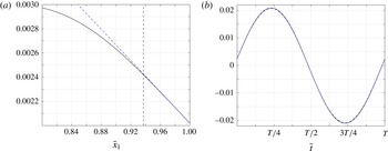
Figure 11. Effect of
 $\bar{\unicode[STIX]{x1D6FC}}$
on the free-end layer: comparison between
$\bar{\unicode[STIX]{x1D6FC}}$
on the free-end layer: comparison between
 $\bar{\unicode[STIX]{x1D709}}(\bar{x}_{1},\bar{t})$
(black solid lines) and
$\bar{\unicode[STIX]{x1D709}}(\bar{x}_{1},\bar{t})$
(black solid lines) and
 $\bar{\unicode[STIX]{x1D709}}_{free}(\bar{x}_{1},\bar{t})$
(dashed blue lines) in the vicinity of the free end
$\bar{\unicode[STIX]{x1D709}}_{free}(\bar{x}_{1},\bar{t})$
(dashed blue lines) in the vicinity of the free end
 $\bar{x}_{1}=1$
for
$\bar{x}_{1}=1$
for
 $\bar{\unicode[STIX]{x1D714}}_{h}=8,\bar{\unicode[STIX]{x1D700}}=10^{-4}$
and
$\bar{\unicode[STIX]{x1D714}}_{h}=8,\bar{\unicode[STIX]{x1D700}}=10^{-4}$
and
 $\bar{\unicode[STIX]{x1D6FC}}=0.02$
. Panel (a) presents
$\bar{\unicode[STIX]{x1D6FC}}=0.02$
. Panel (a) presents
 $\bar{x}_{1}$
-distributions of the fields at
$\bar{x}_{1}$
-distributions of the fields at
 $\bar{t}=\bar{T}$
, with the vertical dashed line marking the upstream end of the free-end layer,
$\bar{t}=\bar{T}$
, with the vertical dashed line marking the upstream end of the free-end layer,
 $\bar{x}_{1}=1-\bar{\unicode[STIX]{x1D6FF}}_{free}$
. Panel (b) shows the counterpart time variations along a period at
$\bar{x}_{1}=1-\bar{\unicode[STIX]{x1D6FF}}_{free}$
. Panel (b) shows the counterpart time variations along a period at
 $\bar{x}_{1}=1-\bar{\unicode[STIX]{x1D6FF}}_{free}$
.
$\bar{x}_{1}=1-\bar{\unicode[STIX]{x1D6FF}}_{free}$
.
To examine the validity of the free-end approximation, figures 8–11 present comparison between the full numerical solution
 $\bar{\unicode[STIX]{x1D709}}(\bar{x}_{1},\bar{t})$
and approximate
$\bar{\unicode[STIX]{x1D709}}(\bar{x}_{1},\bar{t})$
and approximate
 $\bar{\unicode[STIX]{x1D709}}_{free}(\bar{x}_{1},\bar{t})$
prediction in the vicinity of
$\bar{\unicode[STIX]{x1D709}}_{free}(\bar{x}_{1},\bar{t})$
prediction in the vicinity of
 $\bar{x}_{1}=1$
. The results are presented for
$\bar{x}_{1}=1$
. The results are presented for
 $\bar{\unicode[STIX]{x1D714}}_{h}=2$
(figure 8),
$\bar{\unicode[STIX]{x1D714}}_{h}=2$
(figure 8),
 $\bar{\unicode[STIX]{x1D714}}_{h}=4$
(figure 9) and
$\bar{\unicode[STIX]{x1D714}}_{h}=4$
(figure 9) and
 $\bar{\unicode[STIX]{x1D714}}_{h}=8$
(figure 11), with varying values of
$\bar{\unicode[STIX]{x1D714}}_{h}=8$
(figure 11), with varying values of
 $\bar{\unicode[STIX]{x1D700}}$
and
$\bar{\unicode[STIX]{x1D700}}$
and
 $\bar{\unicode[STIX]{x1D6FC}}$
, and for a fixed value of
$\bar{\unicode[STIX]{x1D6FC}}$
, and for a fixed value of
 $\bar{\unicode[STIX]{x1D700}}=0.1$
and varying
$\bar{\unicode[STIX]{x1D700}}=0.1$
and varying
 $\bar{\unicode[STIX]{x1D714}}_{h}$
(figure 10). Each figure shows
$\bar{\unicode[STIX]{x1D714}}_{h}$
(figure 10). Each figure shows
 $\bar{x}_{1}$
-distributions of the fields at fixed times, and time variations of the solutions along a period at the upstream edge of the layer,
$\bar{x}_{1}$
-distributions of the fields at fixed times, and time variations of the solutions along a period at the upstream edge of the layer,
 $\bar{x}_{1}=1-\bar{\unicode[STIX]{x1D6FF}}_{free}$
. In the former, the dashed vertical lines mark the upstream edges of the layer. Figures 8–10 also present counterpart results for a membrane. Figure 11 does not contain
$\bar{x}_{1}=1-\bar{\unicode[STIX]{x1D6FF}}_{free}$
. In the former, the dashed vertical lines mark the upstream edges of the layer. Figures 8–10 also present counterpart results for a membrane. Figure 11 does not contain
 $\bar{\unicode[STIX]{x1D709}}_{mem}(\bar{x}_{1},\bar{t})$
, as the membrane deflection becomes large and non-harmonic at the
$\bar{\unicode[STIX]{x1D709}}_{mem}(\bar{x}_{1},\bar{t})$
, as the membrane deflection becomes large and non-harmonic at the
 $(\bar{\unicode[STIX]{x1D714}}_{h},\bar{\unicode[STIX]{x1D6FC}})$
combination considered.
$(\bar{\unicode[STIX]{x1D714}}_{h},\bar{\unicode[STIX]{x1D6FC}})$
combination considered.
Starting with figure 8, we observe the effect of
 $\bar{\unicode[STIX]{x1D700}}$
, which extends the layer width at increasing values. This effect appears well captured by the dashed vertical lines, and visible deviations between the numerical solution and linear approximation are observed only for
$\bar{\unicode[STIX]{x1D700}}$
, which extends the layer width at increasing values. This effect appears well captured by the dashed vertical lines, and visible deviations between the numerical solution and linear approximation are observed only for
 $\bar{x}_{1}<1-\bar{\unicode[STIX]{x1D6FF}}_{free}$
. While the linear approximation is valid in a relatively narrow layer of
$\bar{x}_{1}<1-\bar{\unicode[STIX]{x1D6FF}}_{free}$
. While the linear approximation is valid in a relatively narrow layer of
 $\bar{\unicode[STIX]{x1D6FF}}_{free}\approx 0.071$
for
$\bar{\unicode[STIX]{x1D6FF}}_{free}\approx 0.071$
for
 $\bar{\unicode[STIX]{x1D700}}=10^{-4}$
, it extends to nearly one fifth of the filament chord,
$\bar{\unicode[STIX]{x1D700}}=10^{-4}$
, it extends to nearly one fifth of the filament chord,
 $\bar{\unicode[STIX]{x1D6FF}}_{free}\approx 0.398$
, for
$\bar{\unicode[STIX]{x1D6FF}}_{free}\approx 0.398$
, for
 $\bar{\unicode[STIX]{x1D700}}=10^{-1}$
. In line with the discussion in § 4, the differences between the filament and the membrane displacements increase with
$\bar{\unicode[STIX]{x1D700}}=10^{-1}$
. In line with the discussion in § 4, the differences between the filament and the membrane displacements increase with
 $\bar{\unicode[STIX]{x1D700}}$
. These differences do not vanish outside the layer, indicating the non-negligible effects of bending rigidity and free-end conditions along the entire filament for
$\bar{\unicode[STIX]{x1D700}}$
. These differences do not vanish outside the layer, indicating the non-negligible effects of bending rigidity and free-end conditions along the entire filament for
 $\bar{\unicode[STIX]{x1D714}}_{h}\gtrsim 1$
.
$\bar{\unicode[STIX]{x1D714}}_{h}\gtrsim 1$
.
Comparing between the results in figures 8 and 9, we observe that the increased value of
 $\bar{\unicode[STIX]{x1D714}}_{h}$
in figure 9 results in a thinner layer. This can be viewed by examining the differences between each of the plots in figure 8(a,c,e), and their counterparts in figure 9(a,c,e), respectively. To further demonstrate this trend, figure 10 shows the layer thinning with increasing
$\bar{\unicode[STIX]{x1D714}}_{h}$
in figure 9 results in a thinner layer. This can be viewed by examining the differences between each of the plots in figure 8(a,c,e), and their counterparts in figure 9(a,c,e), respectively. To further demonstrate this trend, figure 10 shows the layer thinning with increasing
 $\bar{\unicode[STIX]{x1D714}}_{h}$
at constant
$\bar{\unicode[STIX]{x1D714}}_{h}$
at constant
 $\bar{\unicode[STIX]{x1D700}}=0.1$
, starting with
$\bar{\unicode[STIX]{x1D700}}=0.1$
, starting with
 $\bar{\unicode[STIX]{x1D6FF}}_{free}\approx 0.562$
at
$\bar{\unicode[STIX]{x1D6FF}}_{free}\approx 0.562$
at
 $\bar{\unicode[STIX]{x1D714}}_{h}=1$
, and decreasing to
$\bar{\unicode[STIX]{x1D714}}_{h}=1$
, and decreasing to
 $\bar{\unicode[STIX]{x1D6FF}}_{free}\approx 0.325$
at
$\bar{\unicode[STIX]{x1D6FF}}_{free}\approx 0.325$
at
 $\bar{\unicode[STIX]{x1D714}}_{h}=3$
. Physically, the increased inertial effects occurring at higher
$\bar{\unicode[STIX]{x1D714}}_{h}=3$
. Physically, the increased inertial effects occurring at higher
 $\bar{\unicode[STIX]{x1D714}}_{h}$
result in increased
$\bar{\unicode[STIX]{x1D714}}_{h}$
result in increased
 $\bar{x}_{1}$
-gradients along the filament chord, which, in turn, confine the linear approximation to a narrower layer. Inspecting the differences between the beam and membrane deflections, we find, as in previous figures, that they are larger for
$\bar{x}_{1}$
-gradients along the filament chord, which, in turn, confine the linear approximation to a narrower layer. Inspecting the differences between the beam and membrane deflections, we find, as in previous figures, that they are larger for
 $\bar{\unicode[STIX]{x1D714}}_{h}=4$
in figure 9 compared with
$\bar{\unicode[STIX]{x1D714}}_{h}=4$
in figure 9 compared with
 $\bar{\unicode[STIX]{x1D714}}_{h}=2$
in figure 8, reflecting the slower
$\bar{\unicode[STIX]{x1D714}}_{h}=2$
in figure 8, reflecting the slower
 $\bar{\unicode[STIX]{x1D700}}$
convergence between the solutions at increasing actuation frequencies. The presentation of results is concluded with figure 11, showing the effect of decreasing
$\bar{\unicode[STIX]{x1D700}}$
convergence between the solutions at increasing actuation frequencies. The presentation of results is concluded with figure 11, showing the effect of decreasing
 $\bar{\unicode[STIX]{x1D6FC}}$
from its
$\bar{\unicode[STIX]{x1D6FC}}$
from its
 $\bar{\unicode[STIX]{x1D6FC}}=0.2$
value to
$\bar{\unicode[STIX]{x1D6FC}}=0.2$
value to
 $\bar{\unicode[STIX]{x1D6FC}}=0.02$
. For a given filament, a decrease in
$\bar{\unicode[STIX]{x1D6FC}}=0.02$
. For a given filament, a decrease in
 $\bar{\unicode[STIX]{x1D6FC}}$
is equivalent to reducing the incoming flow speed (see (3.3)), which, in turn, diminishes the amplitudes of both inertia and pressure loading terms in the equation of motion (3.1). This stabilizing effect is reflected by an
$\bar{\unicode[STIX]{x1D6FC}}$
is equivalent to reducing the incoming flow speed (see (3.3)), which, in turn, diminishes the amplitudes of both inertia and pressure loading terms in the equation of motion (3.1). This stabilizing effect is reflected by an
 $\bar{\unicode[STIX]{x1D6FC}}^{-1/4}$
thickening of the free-end layer (see (5.17)), as confirmed by the results in the figure.
$\bar{\unicode[STIX]{x1D6FC}}^{-1/4}$
thickening of the free-end layer (see (5.17)), as confirmed by the results in the figure.
The free-end approximation (5.18) depends on numerical evaluation of
 $\bar{\unicode[STIX]{x1D709}}_{FE}$
and
$\bar{\unicode[STIX]{x1D709}}_{FE}$
and
 $(\unicode[STIX]{x2202}\unicode[STIX]{x1D709}/\unicode[STIX]{x2202}\bar{x}_{1})_{FE}$
, yet its main significance is in correctly predicting the extent to which the linear description holds. A similar argument is in place in the context of the actuated-layer analysis in § 5.2.1, where numerical patching has been applied. In view of the complex nonlinear fluid–structure interaction involved, we consider these estimates for the body motion, as well as the leading-order balances identified near the edges, valuable.
$(\unicode[STIX]{x2202}\unicode[STIX]{x1D709}/\unicode[STIX]{x2202}\bar{x}_{1})_{FE}$
, yet its main significance is in correctly predicting the extent to which the linear description holds. A similar argument is in place in the context of the actuated-layer analysis in § 5.2.1, where numerical patching has been applied. In view of the complex nonlinear fluid–structure interaction involved, we consider these estimates for the body motion, as well as the leading-order balances identified near the edges, valuable.
6 Conclusion
We studied the fluid–structure interaction of a ‘hanging flag’, a vertically hanging filament immersed in uniform incompressible flow, subject to small-amplitude harmonic heaving at its upstream end. Focusing on the limit of small flexural rigidity, we examined the differences between a highly elastic beam (where bending rigidity is small but finite) and a membrane (where bending rigidity vanishes). The problem was analysed by means of potential thin airfoil theory in conjunction with a discrete vortex model for the downstream wake. Initially, it was verified that the beam deflection and associated flow field converge to the membrane solution at small bending rigidities,
 $\bar{\unicode[STIX]{x1D700}}\rightarrow 0$
. At low actuation frequencies, the differences between the membrane and beam motions were found small, as both are displaced in a nearly rigid-body motion parallel to the upstream-edge actuation. With increasing frequency, the differences between the beam and the membrane systems become visible at increasingly lower values of
$\bar{\unicode[STIX]{x1D700}}\rightarrow 0$
. At low actuation frequencies, the differences between the membrane and beam motions were found small, as both are displaced in a nearly rigid-body motion parallel to the upstream-edge actuation. With increasing frequency, the differences between the beam and the membrane systems become visible at increasingly lower values of
 $\bar{\unicode[STIX]{x1D700}}$
, and the stabilizing effect of beam flexural rigidity, resulting in reduced flapping amplitudes, was observed. Examining the beam motion near its edge points at non-small frequencies, semi-analytic approximations for the associated time-periodic displacements were obtained. Close to the actuated end, a layer of width
$\bar{\unicode[STIX]{x1D700}}$
, and the stabilizing effect of beam flexural rigidity, resulting in reduced flapping amplitudes, was observed. Examining the beam motion near its edge points at non-small frequencies, semi-analytic approximations for the associated time-periodic displacements were obtained. Close to the actuated end, a layer of width
 $\bar{\unicode[STIX]{x1D700}}^{1/2}$
was identified, where the flexural rigidity and tension terms in the equation of motion were balanced. Here, the differences between the beam and membrane deflections were attributed to the additional zero-slope condition satisfied by the beam. In the vicinity of the free end, a local Taylor expansion was carried out. A balance between the bending and inertia terms resulted in a layer of width
$\bar{\unicode[STIX]{x1D700}}^{1/2}$
was identified, where the flexural rigidity and tension terms in the equation of motion were balanced. Here, the differences between the beam and membrane deflections were attributed to the additional zero-slope condition satisfied by the beam. In the vicinity of the free end, a local Taylor expansion was carried out. A balance between the bending and inertia terms resulted in a layer of width
 $\propto \bar{\unicode[STIX]{x1D700}}^{1/4}/\bar{\unicode[STIX]{x1D714}}_{h}^{1/2}$
. The free-end layer is thus thicker than the upstream-end layer for
$\propto \bar{\unicode[STIX]{x1D700}}^{1/4}/\bar{\unicode[STIX]{x1D714}}_{h}^{1/2}$
. The free-end layer is thus thicker than the upstream-end layer for
 $\bar{\unicode[STIX]{x1D714}}_{h}\approx 1$
, and becomes thinner with increasing
$\bar{\unicode[STIX]{x1D714}}_{h}\approx 1$
, and becomes thinner with increasing
 $\bar{\unicode[STIX]{x1D714}}_{h}$
. Within the layer, the beam deflects linearly with the distance from the edge, in marked difference from a membrane.
$\bar{\unicode[STIX]{x1D714}}_{h}$
. Within the layer, the beam deflects linearly with the distance from the edge, in marked difference from a membrane.
A main objective of the present work was to examine the effect of small structural bending stiffness, in the presence of a non-small tension force, on the dynamical behaviour of the system. In this respect, the inspection of the convergence of the beam deflection and resulting flow field to the membrane solution, together with the approximate analysis of the beam edges motion, complies with the research goal. While the nonlinear fluid–structure interaction problem involved has obviated closed-form matching of ‘inner layer’ to ‘outer’ descriptions, we consider the numerical patching, as a means for validating the approximate description, valuable. Importantly, the matching of the layers was made with the full numerical solution for a beam and not for a membrane. This is since, for
 $\bar{\unicode[STIX]{x1D714}}_{h}\gtrsim 1$
, non-small
$\bar{\unicode[STIX]{x1D714}}_{h}\gtrsim 1$
, non-small
 $\bar{x}_{1}$
-gradients of the displacement (driven by growing inertial effects) occur along the entire filament, causing the bending rigidity term, and associated deviations between the membrane and beam motions, to occupy the entire body chord (see, e.g. figures 2
b and 4
d).
$\bar{x}_{1}$
-gradients of the displacement (driven by growing inertial effects) occur along the entire filament, causing the bending rigidity term, and associated deviations between the membrane and beam motions, to occupy the entire body chord (see, e.g. figures 2
b and 4
d).
The set-up considered in this work, of a hanging flag actuated at its upstream end by harmonic heaving motion, has allowed for a detailed analysis of the system response at specified frequencies. While this has assisted in rationalizing our findings, the analysis is limited to choices of
 $\bar{\unicode[STIX]{x1D714}}_{h}$
where the system acquires a final periodic state. Additional results, not presented here, indicate that, for a given combination of the problem parameters
$\bar{\unicode[STIX]{x1D714}}_{h}$
where the system acquires a final periodic state. Additional results, not presented here, indicate that, for a given combination of the problem parameters
 $\bar{\unicode[STIX]{x1D707}},\bar{\unicode[STIX]{x1D6FC}}$
and
$\bar{\unicode[STIX]{x1D707}},\bar{\unicode[STIX]{x1D6FC}}$
and
 $\bar{\unicode[STIX]{x1D700}}$
, there exists a critical value of
$\bar{\unicode[STIX]{x1D700}}$
, there exists a critical value of
 $\bar{\unicode[STIX]{x1D714}}_{h}$
above which the system response becomes non-periodic, and the body displacement is non-small. The mapping of these states, as well as the analysis of the associated system dynamics, are not in the scope of the present work. Noting this limitation, the current scheme may be readily applied to analyse the system response to any subcritical (periodic or non-periodic) forcing, characterized by long enough time scales. Further study on the counterpart hanging flag eigenvalue problem, as well as investigation of the effect of varying the actuated-free edge conditions conditions on the results, are topics for future work.
$\bar{\unicode[STIX]{x1D714}}_{h}$
above which the system response becomes non-periodic, and the body displacement is non-small. The mapping of these states, as well as the analysis of the associated system dynamics, are not in the scope of the present work. Noting this limitation, the current scheme may be readily applied to analyse the system response to any subcritical (periodic or non-periodic) forcing, characterized by long enough time scales. Further study on the counterpart hanging flag eigenvalue problem, as well as investigation of the effect of varying the actuated-free edge conditions conditions on the results, are topics for future work.


