


1. Introduction
Over the last few decades, considerable research efforts have been devoted to studying the stability of natural convection in a vertical porous slab because of its applications in the analysis of contaminant diffusion in the soil, the extraction of hydrocarbons, the CO2 sequestration processes, the use of metal foams for the optimized design of heat exchangers, the design of packed bed reactors, building insulation involving an unventilated air gap and for breathing walls to chemical engineering to mention a few.
The first proof that a vertical porous slab of Darcy type with constant permeability, which is held at fixed but different temperatures on the impermeable vertical walls, is stable to perturbations from the equilibrium state was presented by Gill (Reference Gill1969). Subsequently, several articles were dealt with other extensions on Gill's problem (Wolanski Reference Wolanski1973; Rees Reference Rees1988, Reference Rees2011; Straughan Reference Straughan1988; Flavin & Rionero Reference Flavin and Rionero1999; Scott & Straughan Reference Scott and Straughan2013; Barletta & De B. Alves Reference Barletta and De B. Alves2014). All these studies revealed that no instability is possible in the sense that the basic solution is always linearly stable to two-dimensional disturbances no matter how large the Darcy–Rayleigh number is and thus complemented the results of Gill (Reference Gill1969). The state-of-the-art has been summarized in a monograph by Nield & Bejan (Reference Nield and Bejan2017).
The proof of stability drawn in Gill's paper is shown to be ineffective if the vertical boundaries are considered as permeable instead of impermeable and it was also displayed that the basic state becomes unstable when the Darcy–Rayleigh number is larger than 197.081 (Barletta Reference Barletta2015). This work motivated many investigators to extend the study by including other effects such as an internal heat source (Barletta Reference Barletta2016; Barletta & Celli Reference Barletta and Celli2017), local thermal non-equilibrium (Celli, Barletta & Rees Reference Celli, Barletta and Rees2017) and anisotropy (Barletta & Celli Reference Barletta and Celli2021). Furthermore, the problem of Gill was analysed for an Oldroyd-B type of viscoelastic fluid (Shankar & Shivakumara Reference Shankar and Shivakumara2017), Brinkman model (Shankar, Kumar & Shivakumara Reference Shankar, Kumar and Shivakumara2017), maximum density effect (Naveen, Shankar & Shivakumara Reference Naveen, Shankar and Shivakumara2020), second diffusing component (Shankar, Naveen & Shivakumara Reference Shankar, Naveen and Shivakumara2022) and the possibility of the basic flow becoming unstable was established in all these cases.
Another important topic that has attracted the attention of researchers in recent years is the study of thermal convective instability in a heterogeneous porous medium. This is because the permeability of the porous materials encountered in many practical situations is heterogeneous, such as the artificial porous materials like pellets used in chemical engineering processes, fibre material used for the insulating purposes and in many geological systems. It is shown experimentally that the porosity near a solid wall is not a constant but varies, due to which the permeability also varies (Schwartz & Smith Reference Schwartz and Smith1953, Roblee, Baird & Tierney Reference Roblee, Baird and Tierney1958; Benenati & Brosilow Reference Benenati and Brosilow1962). Since then, the significance and importance of heterogeneity for various aspects of convection in porous media have been continued to be recognized by scientists and engineers. The study of natural convection in horizontal porous media with variable permeability has been studied extensively (Nield & Kuznetsov Reference Nield and Kuznetsov2007; Nield Reference Nield2008; Rionero Reference Rionero2011; Barletta, Celli & Kuznetsov Reference Barletta, Celli and Kuznetsov2012; Barletta & Nield Reference Barletta and Nield2012). It has been observed that the effect of heterogeneity of the permeability has a noticeable impact in promoting the onset of instability.
On the other hand, Braester & Vadasz (Reference Braester and Vadasz1993) considered the effect of the general form of stratification of the porous-medium permeability and thermal conductivity on natural convection and showed that weak heterogeneity in permeability plays a relatively passive role. Rees & Pop (Reference Rees and Pop2000) studied the effect of exponentially decaying permeability on free convective boundary-layer flow induced by a vertical heated surface embedded in a porous medium and held at a constant temperature. It was found that, near the leading edge, the flow is enhanced and the rate of heat transfer is much higher than in the uniform permeability case. The effect of spatial discretization and different types of heterogeneous hydraulic conductivity fields on free thermal convection was examined by Nguyen, Graf & Guevara Morel (Reference Nguyen, Graf and Guevara Morel2016). The global sensitivity analysis and uncertainty quantification were used to study natural convection in heterogeneous porous media, including velocity-dependent dispersion by Fajraoui et al. (Reference Fajraoui, Fahs, Younes and Sudret2017). Salibindla et al. (Reference Salibindla, Subedi, Shen, Masuk and Ni2018) conducted an experimental investigation of the dissolution convection in a porous medium with multiscale heterogeneity and some important implications for the future estimation of subsurface carbon sequestration were presented. Shafabakhsh et al. (Reference Shafabakhsh, Fahs, Ataie-Ashtiani and Simmons2019) considered the influence of a fractured heterogeneity effect on unstable density-driven flow. It was shown that the onset of instability and free convection occur with a lower critical Rayleigh number, indicating the fractured networks have a destabilizing effect. Benham, Bickle & Neufeld (Reference Benham, Bickle and Neufeld2021) studied the effect of vertical heterogeneity in a porous medium on the overall flow properties by way of upscaling and illustrated how and when heterogeneities accelerate/decelerate the dynamic flow. The effect of permeability variation on natural convection in a vertical porous layer subjected to constant heat fluxes along the sidewalls was investigated by Damene et al. (Reference Damene, Alloui, Alloui and Vasseur2021). The results for the flow field, temperature distribution and heat transfer rates were presented for various forms of the variable permeability cases.
As envisaged by the previous studies, flows in porous media are particular in that the velocity field and heat transfer are largely dictated by the medium properties. Practically every porous domain exhibits heterogeneity with respect to permeability. It is thus imperative to establish the implications of horizontal heterogeneities in controlling the onset, growth and/or decay of thermal instabilities in a vertical porous layer, which have not received any attention to the best of our knowledge. The intent of the present study is to quantify the effect of both weak and strong heterogeneities of the permeability on the stability of natural convection in a vertical Darcy porous layer. In the discussion, three different models of permeability functions are considered viz. linear, quadratic and exponential. The stability of basic parallel buoyant flow for these models is analysed by adopting a modal analysis. The stability eigenvalue problem is solved numerically by employing the Chebyshev collocation method. The effects of different models of heterogeneities on the stability/instability characteristics are discussed for the neutral stability curves and for the critical values of the Darcy–Rayleigh number, wavenumber and wave speed.
2. Mathematical formulation
An infinite vertical porous slab of width  $2h$ saturated with an incompressible Newtonian fluid and bounded by a pair of impermeable left
  $({x^ \ast } ={-} h)$ and right
  $({x^\ast } = h)$ vertical walls which are maintained at constant temperatures
  ${T_1}$ and
  ${T_2}( > {T_1})$, respectively is considered (see figure 1). The origin of the coordinate axes is taken in the middle of the slab with the
  ${z^\ast }$-axis pointing vertically upward and the gravitational acceleration
  $\boldsymbol{g}$ is acting in the negative
  ${z^\ast }$ direction, while the
  ${x^ \ast }$- and
  ${y^ \ast }$-axes are horizontal. The flow in the Darcy porous medium is driven by the buoyancy force due to the temperature difference between the vertical walls. The local thermodynamic equilibrium and the Oberbeck–Boussinesq approximation are assumed. Besides, the permeability of the porous medium is assumed to vary horizontally within the porous medium. With asterisks being used to denote the dimensional variables, the governing equations describing the system behaviour are
 \begin{gather}{\nabla ^ \ast }\boldsymbol{\cdot }{\boldsymbol{u}^ \ast } = 0,\end{gather}
 \begin{gather}- {\nabla ^ \ast }{P^ \ast } + {\rho _0}\beta ({T^ \ast } - {T_0})g\hat{k} - \frac{\mu }{{{K^ \ast }({x^ \ast })}}{\boldsymbol{u}^ \ast } = 0,\end{gather}
 \begin{gather}\chi \frac{{\partial {T^ \ast }}}{{\partial {t^ \ast }}} + ({\boldsymbol{u}^ \ast }\boldsymbol{\cdot }{\nabla ^ \ast }){T^ \ast } = \kappa {\nabla ^{ {\ast} 2}}{T^ \ast }.\end{gather}
In the above equations,  ${\boldsymbol{u}^ \ast } = ({u^ \ast },{v^ \ast },{w^ \ast })$ is the filtration velocity,
  ${P^ \ast }$ is the pressure,
  ${\rho _0}$ is the density at the reference temperature
  ${T_0} = ({T_1} + {T_2})/2$,
  $\beta$ is the volumetric thermal expansion coefficient,
  ${T^ \ast }$ is the temperature,
  $\mu$ is the viscosity of the fluid,
  ${K^ \ast }({x^ \ast })$ is the horizontally varying permeability function,
  $\chi$ is the ratio of heat capacities and
  $\kappa$ is the thermal diffusivity.

Figure 1. Physical configuration.
The boundary conditions are:
 \begin{equation}{u^ \ast } = 0\;\textrm{at}\;{x^ \ast } ={\pm} h;\quad {T^ \ast } = {T_1}\;\textrm{at}\;{x^ \ast } ={-} h;\quad {T^ \ast } = {T_2}\;\textrm{at}\;{x^ \ast } = h.\end{equation}
We non-dimensionalize the above equations through the transformation
 \begin{align}\boldsymbol{\nabla
} &= h{\nabla ^\ast },\quad \boldsymbol{u} =
\frac{{{\boldsymbol{u}^ \ast }}}{{(\kappa /h)}},\quad P =
\frac{{{P^ \ast }}}{{(\mu \kappa /{K_0})}},\quad t =
\frac{{{t^ \ast }}}{{(\chi {h^2}/\kappa )}}.\nonumber\\
T &=
\frac{{({T^ \ast } - {T_0})}}{{({T_2} - {T_1})}},\quad K(x)
= \frac{{{K^\ast }({x^ \ast })}}{{{K_0}}},\end{align}
\begin{align}\boldsymbol{\nabla
} &= h{\nabla ^\ast },\quad \boldsymbol{u} =
\frac{{{\boldsymbol{u}^ \ast }}}{{(\kappa /h)}},\quad P =
\frac{{{P^ \ast }}}{{(\mu \kappa /{K_0})}},\quad t =
\frac{{{t^ \ast }}}{{(\chi {h^2}/\kappa )}}.\nonumber\\
T &=
\frac{{({T^ \ast } - {T_0})}}{{({T_2} - {T_1})}},\quad K(x)
= \frac{{{K^\ast }({x^ \ast })}}{{{K_0}}},\end{align}
where  ${K_0}$ is a reference permeability at the centre of the porous slab. In analysing instability problems akin to the present investigation, Barletta (Reference Barletta2015), Barletta, Celli & Ouarzazi (Reference Barletta, Celli and Ouarzazi2017) and Shankar, Shivakumara & Naveen (Reference Shankar, Shivakumara and Naveen2021) have established the validity of Squire's theorem (i.e. two-dimensional disturbances are more unstable than the three-dimensional ones). Motivated by these findings, we have restricted our attention purely to two-dimensional analysis and accordingly the streamfunction
  ${\psi ^ \ast }({x^ \ast },{z^ \ast },{t^ \ast })$ is introduced through
  ${u^ \ast } = \partial {\psi ^\ast }/\partial {z^ \ast }$ and
  ${w^ \ast } ={-} \partial {\psi ^\ast }/\partial {x^ \ast }$. The pressure term is then eliminated from the momentum equation by operating curl and the following dimensionless equations are obtained:
 \begin{gather}\frac{1}{{K(x)}}{\nabla ^2}\psi - \frac{{DK(x)}}{{{{[K(x)]}^2}}}\frac{{\partial \psi }}{{\partial x}} ={-} {R_D}\frac{{\partial T}}{{\partial x}},\end{gather}
 \begin{gather}\frac{{\partial T}}{{\partial t}} - J(\psi ,T) = {\nabla ^2}T,\end{gather}
where D denotes the derivative with respect to x,  ${R_D} = \beta gh{K_0}({T_2} - {T_1})/\nu \kappa$ is the Darcy–Rayleigh number,
  $J(\psi ,T) = (\partial \psi /\partial x)(\partial T/\partial z) - (\partial \psi /\partial z)(\partial T/\partial x)$ is the Jacobian and
  $\nu = \mu /{\rho _0}$ is the kinematic viscosity.
The boundary conditions now become
 \begin{equation}\psi = 0\;\textrm{at}\;x ={\pm} 1\quad \textrm{and}\quad T ={\pm} {\textstyle{1 \over 2}}\;\textrm{at}\;x ={\pm} 1.\end{equation}
It is convenient to introduce the following modified Darcy–Rayleigh number based on the average permeability  $\bar{K}(x)$ as
  ${\tilde{R}_D} = \beta gh\bar{K}(x)({T_2} - {T_1})/\nu \kappa$, where
  $\bar{K}(x) = b{K_0}$ with
 \begin{equation}b = \frac{1}{2}\int_{ - 1}^1 {K(x)\,\textrm{d}\kern0.7pt x} .\end{equation}
The Darcy–Rayleigh number is related to the modified Darcy–Rayleigh number  ${\tilde{R}_D}$ by the following expression:
 \begin{equation}{\tilde{R}_D} = b{R_D}.\end{equation}
Natural and man-made porous domains exhibit heterogeneity in permeability and it can vary by many orders of magnitude and sometimes rapidly over small spatial scales. As such, the prediction of weak and strong heterogeneities in controlling the growth and/or decay of instabilities may turn out to be important in many of the engineering applications mentioned earlier. Accordingly, the following heterogeneity models, with m being the variable permeability constant, are considered:
Linear heterogeneity of the permeability
(2.11) \begin{equation}K(x) = 1 + mx;\quad b = 1.\end{equation}
Quadratic heterogeneity of the permeability
(2.12)\begin{equation}K(x) = 1 + m{x^2};\quad b = 1 + m/3.\end{equation}Exponential heterogeneity of the permeability
(2.13)\begin{equation}K(x) = {\textrm{e}^{mx}};\quad b = \sinh m/m.\end{equation}


3. Base state
The base state, about which the linear stability characteristics will be analysed, corresponds to a steady, parallel, fully developed flow. Base state quantities are designated by suffix b, and also  ${\psi _b}$ and
  ${T_b}$ are considered to be functions of x alone. Equations (2.6)–(2.8a,b), respectively become
 \begin{gather}\frac{1}{{K(x)}}{D^2}{\psi _b} - \frac{{DK(x)}}{{{{[K(x)]}^2}}}D{\psi _b} ={-} \frac{{{{\tilde{R}}_D}}}{b}D{T_b},\end{gather}
 \begin{gather}{D^2}{T_b} = 0,\end{gather}
 \begin{gather}{\psi _b} = 0\;\textrm{at}\;x ={\pm} 1\quad \textrm{and}\quad {T_b} ={\pm} {\textstyle{1 \over 2}}\;\textrm{at}\;x ={\pm} 1.\end{gather}
The solutions of the above equations obtained analytically for linear, quadratic and exponential heterogeneities of the permeability are, respectively, given by
 \begin{equation}{\psi _b}(x) = \frac{{{{\tilde{R}}_D}}}{{12}}[{m^2} - 2mx - 3]({x^2} - 1),\quad {T_b} = \frac{x}{2}.\end{equation}
 \begin{equation}{\psi _b}(x) ={-} \frac{{{{\tilde{R}}_D}}}{{8(1 + m/3)}}[m({x^2} + 1) + 2]({x^2} - 1),\quad {T_b} = \frac{x}{2}.\end{equation}
 \begin{equation}{\psi _b}(x) = \frac{{{{\tilde{R}}_D}}}{{4\sinh m}}[ - 2\,{\textrm{e}^m} - {\textrm{e}^{m(x + 2)}}(x - 1) + {\textrm{e}^{mx}}(x + 1)](\coth m - 1),\quad {T_b} = \frac{x}{2}.\end{equation}
One may easily check that the basic solution given by (3.4a,b)–(3.6a,b) coincides with that of Gill (Reference Gill1969) when  $m = 0$ (constant permeability). Equations (3.4a,b)–(3.6a,b) reveal that
  ${\psi _b}(x)$ is not symmetric about the
  $z$-axis for linear and exponential, while it is symmetric for quadratic heterogeneities of the permeability. Moreover,
  ${\psi _b}(x)/{\tilde{R}_D}$ remains invariant under the transformation
 \begin{equation}m \to - m,\quad x \to - x,\end{equation}
for linear and exponential heterogeneities of the permeability.
4. Linear stability analysis
We perturb the basic state with small-amplitude disturbances given by
 \begin{equation}\psi = {\psi _b} + \varepsilon \hat{\psi },\quad T = {T_b} + \varepsilon \hat{T},\end{equation}
where the parameter  $\varepsilon$ is such that
  $\varepsilon > 0$ and
  $\varepsilon \ll 1$, while
  $\hat{\psi }$ and
  $\hat{T}$ are the perturbation fields. We assume the perturbed streamfunction and temperature have the form of normal modes
 \begin{equation}(\hat{\psi },\hat{T})(x,z,t) = (\varPsi ,\varTheta )(x)\,{\textrm{e}^{\textrm{i}a(z - ct)}},\end{equation}
where a is the vertical wavenumber and  $c = {c_r} + i{c_i}$ is the complex wave speed. The growth rate
  ${c_i}$ marks the difference between stability
  $({c_i} < 0)$ and instability
  $({c_i} > 0)$. The neutrally stable configuration is identified by
  ${c_i} = 0$. Substituting equations (4.1a,b) and (4.2) into (2.6)–(2.8a,b), we obtain the following eigenvalue problem for neutrally stable modes:
 \begin{gather}\frac{1}{{K(x)}}({D^2} - {a^2})\varPsi - \frac{{DK(x)}}{{{{[K(x)]}^2}}}D\varPsi + \frac{{{{\tilde{R}}_D}}}{b}D\varTheta = 0,\end{gather}
 \begin{gather}ia({\textstyle{1 \over 2}}\varPsi - D{\psi _b}\varTheta ) - ({D^2} - {a^2})\varTheta = iac\varTheta ,\end{gather}
 \begin{gather}\varPsi = \varTheta = 0\;\textrm{at}\;x ={\pm} 1.\end{gather}
We note that the above eigenvalue problem is endowed with symmetry if  $K(x)$ varies linearly and exponentially, and in which cases (4.3)–(4.5) are left invariant by the transformation
 \begin{equation}\varPsi \to - \varPsi ,\quad x \to - x,\quad m \to - m,\quad a \to - a,\quad c \to - c.\end{equation}
5. Gill's growth rate analysis
It is not out of place to attempt to determine whether Gill's proof of linear stability for constant permeability can be extended to the cases of horizontal heterogeneity models of the permeability. Following the analysis of Gill (Reference Gill1969), we operate  $(1/K(x))({D^2} - {a^2}) - (DK(x)/{[K(x)]^2})D$ on (4.4) to eliminate
  $\varPsi$ and obtain a single fourth-order differential equation for
  $\varTheta$ in the form
 \begin{equation}\begin{array}{ccccc}
& - \dfrac{{ia{{\tilde{R}}_D}}}{{2b}}\varTheta ^{\prime} -
ia\left\{ \dfrac{1}{{K(x)}}({{\psi^{\prime\prime\prime}}_b}\varTheta
+ 2{{\psi^{\prime\prime}}_b}\varTheta^{\prime} +
{{\psi^{\prime}}_b}\varTheta^{\prime\prime} \right.\\
&\hspace{9pc}\left.- {a^2}{{\psi^{\prime}}_b}\varTheta ) -
\dfrac{{K^{\prime}(x)}}{{{{[K(x)]}^2}}}({{\psi^{\prime\prime}}_b}\varTheta
+ {{\psi^{\prime}}_b}\varTheta^{\prime}) \right\}\\
& \quad - \dfrac{1}{{K(x)}}(\varTheta
^{\prime\prime\prime\prime} + {a^4}\varTheta -
2{a^2}\varTheta ^{\prime\prime}) +
\dfrac{{K^{\prime}(x)}}{{{{[K(x)]}^2}}}(\varTheta
^{\prime\prime\prime} - {a^2}\varTheta ^{\prime}) \\
& \hspace{5pc}= iac\left\{ {\dfrac{1}{{K(x)}}(\varTheta^{\prime\prime} -
{a^2}\varTheta ) -
\dfrac{{K^{\prime}(x)}}{{{{[K(x)]}^2}}}\varTheta^{\prime}}
\right\},
\end{array}\end{equation}
\begin{equation}\begin{array}{ccccc}
& - \dfrac{{ia{{\tilde{R}}_D}}}{{2b}}\varTheta ^{\prime} -
ia\left\{ \dfrac{1}{{K(x)}}({{\psi^{\prime\prime\prime}}_b}\varTheta
+ 2{{\psi^{\prime\prime}}_b}\varTheta^{\prime} +
{{\psi^{\prime}}_b}\varTheta^{\prime\prime} \right.\\
&\hspace{9pc}\left.- {a^2}{{\psi^{\prime}}_b}\varTheta ) -
\dfrac{{K^{\prime}(x)}}{{{{[K(x)]}^2}}}({{\psi^{\prime\prime}}_b}\varTheta
+ {{\psi^{\prime}}_b}\varTheta^{\prime}) \right\}\\
& \quad - \dfrac{1}{{K(x)}}(\varTheta
^{\prime\prime\prime\prime} + {a^4}\varTheta -
2{a^2}\varTheta ^{\prime\prime}) +
\dfrac{{K^{\prime}(x)}}{{{{[K(x)]}^2}}}(\varTheta
^{\prime\prime\prime} - {a^2}\varTheta ^{\prime}) \\
& \hspace{5pc}= iac\left\{ {\dfrac{1}{{K(x)}}(\varTheta^{\prime\prime} -
{a^2}\varTheta ) -
\dfrac{{K^{\prime}(x)}}{{{{[K(x)]}^2}}}\varTheta^{\prime}}
\right\},
\end{array}\end{equation}
where primes denote differentiation with respect to x. We multiply equation (5.1) by  $\bar{\varTheta }$, the complex conjugate of
  $\varTheta$, and integrate it over the domain
  $- 1 \le x \le 1$ to get
 \begin{equation}\begin{array}{ccccc}
&\hspace{-1pc} \displaystyle- \dfrac{{ia{{\tilde{R}}_D}}}{{2b}}\int_{ - 1}^1
{\varTheta
^{\prime}\bar{\varTheta }\,\textrm{d}\kern0.7pt x} - ia\int_{ - 1}^1
\left\{
\dfrac{1}{{K(x)}}({{\psi^{\prime\prime\prime}}_b}|\varTheta
{|^2} + 2{{\psi^{\prime\prime}}_b}\varTheta^{\prime}\bar{\varTheta
} + {{\psi^{\prime}}_b}\varTheta^{\prime\prime}\bar{\varTheta }
- {a^2}{{\psi^{\prime}}_b}|\varTheta {|^2})\right. \\
& \hspace{5pc}\left.-
\dfrac{{K^{\prime}(x)}}{{{{[K(x)]}^2}}}({{\psi^{\prime\prime}}_b}|\varTheta
{|^2} + {{\psi^{\prime}}_b}\varTheta^{\prime}\bar{\varTheta
}) \right\}\textrm{d}\kern0.7pt x \\
& \quad \displaystyle- \int_{ - 1}^1
{\left\{
{\dfrac{1}{{K(x)}}(\varTheta^{\prime\prime\prime\prime}\bar{\varTheta
} + {a^4}|\varTheta {|^2} -
2{a^2}\varTheta^{\prime\prime}\bar{\varTheta }) -
\dfrac{{K^{\prime}(x)}}{{{{[K(x)]}^2}}}({\varTheta^{\prime\prime\prime}\bar{\varTheta
} - {a^2}\varTheta^{\prime}\bar{\varTheta }} )}
\right\}\textrm{d}\kern0.7pt x} \\
& \quad \quad \displaystyle= iac\int_{ - 1}^1
{\left\{
{\dfrac{1}{{K(x)}}(\varTheta^{\prime\prime}\bar{\varTheta }
- {a^2}|\varTheta {|^2}) -
\dfrac{{K^{\prime}(x)}}{{{{[K(x)]}^2}}}\varTheta^{\prime}\bar{\varTheta
}} \right\}\textrm{d}\kern0.7pt x} .
\end{array}\end{equation}
\begin{equation}\begin{array}{ccccc}
&\hspace{-1pc} \displaystyle- \dfrac{{ia{{\tilde{R}}_D}}}{{2b}}\int_{ - 1}^1
{\varTheta
^{\prime}\bar{\varTheta }\,\textrm{d}\kern0.7pt x} - ia\int_{ - 1}^1
\left\{
\dfrac{1}{{K(x)}}({{\psi^{\prime\prime\prime}}_b}|\varTheta
{|^2} + 2{{\psi^{\prime\prime}}_b}\varTheta^{\prime}\bar{\varTheta
} + {{\psi^{\prime}}_b}\varTheta^{\prime\prime}\bar{\varTheta }
- {a^2}{{\psi^{\prime}}_b}|\varTheta {|^2})\right. \\
& \hspace{5pc}\left.-
\dfrac{{K^{\prime}(x)}}{{{{[K(x)]}^2}}}({{\psi^{\prime\prime}}_b}|\varTheta
{|^2} + {{\psi^{\prime}}_b}\varTheta^{\prime}\bar{\varTheta
}) \right\}\textrm{d}\kern0.7pt x \\
& \quad \displaystyle- \int_{ - 1}^1
{\left\{
{\dfrac{1}{{K(x)}}(\varTheta^{\prime\prime\prime\prime}\bar{\varTheta
} + {a^4}|\varTheta {|^2} -
2{a^2}\varTheta^{\prime\prime}\bar{\varTheta }) -
\dfrac{{K^{\prime}(x)}}{{{{[K(x)]}^2}}}({\varTheta^{\prime\prime\prime}\bar{\varTheta
} - {a^2}\varTheta^{\prime}\bar{\varTheta }} )}
\right\}\textrm{d}\kern0.7pt x} \\
& \quad \quad \displaystyle= iac\int_{ - 1}^1
{\left\{
{\dfrac{1}{{K(x)}}(\varTheta^{\prime\prime}\bar{\varTheta }
- {a^2}|\varTheta {|^2}) -
\dfrac{{K^{\prime}(x)}}{{{{[K(x)]}^2}}}\varTheta^{\prime}\bar{\varTheta
}} \right\}\textrm{d}\kern0.7pt x} .
\end{array}\end{equation}
The terms in (5.2) rule out the possibility of reaching any definite conclusion in determining whether the sign of  ${c_i}$ is positive or negative. Hence, Gill's analysis of proving the stability becomes ineffective owing to the consideration of horizontal heterogeneity of the permeability. However, for a constant permeability case (
 $K(x) = 1$,
  ${\tilde{R}_D} = {R_D}$ with
  $b = 1$,
  ${\psi _b} = {\psi _b}(x) = {R_D}(1 - {x^2})/4$) the above equation simply reduces to
 \begin{align}&\frac{{ia{R_D}}}{2}
{\int_{ - 1}^1 {x(|\varTheta^{\prime}{|^2} +
{a^2}|\varTheta {|^2})\,\textrm{d}\kern0.7pt x} } + \int_{ -
1}^1 (|\varTheta ^{\prime\prime}{|^2} + {a^4}|\varTheta
{|^2} \nonumber\\
&\qquad \qquad + 2{a^2}|\varTheta ^{\prime}{|^2})\,\textrm{d}\kern0.7pt x =
iac\int_{ - 1}^1 {(|\varTheta ^{\prime}{|^2} +
{a^2}|\varTheta {|^2})\,\textrm{d}\kern0.7pt x}.\end{align}
\begin{align}&\frac{{ia{R_D}}}{2}
{\int_{ - 1}^1 {x(|\varTheta^{\prime}{|^2} +
{a^2}|\varTheta {|^2})\,\textrm{d}\kern0.7pt x} } + \int_{ -
1}^1 (|\varTheta ^{\prime\prime}{|^2} + {a^4}|\varTheta
{|^2} \nonumber\\
&\qquad \qquad + 2{a^2}|\varTheta ^{\prime}{|^2})\,\textrm{d}\kern0.7pt x =
iac\int_{ - 1}^1 {(|\varTheta ^{\prime}{|^2} +
{a^2}|\varTheta {|^2})\,\textrm{d}\kern0.7pt x}.\end{align}
Equating the real part of (5.3) allows one to conclude that  ${c_i} < 0$, indicating that all infinitesimal perturbations decay. This conclusion is in conformity with Gill's classical proof of stability.
6. Numerical procedure
The ensued eigenvalue problem formulated through (4.3)–(4.5) is solved numerically by means of the Chebyshev collocation method as Gill's analysis is ineffective in establishing the stability/instability of the base flow. The Chebyshev polynomial of kth order is given by
 \begin{equation}{\xi _k}(x) = \cos k\theta ,\quad \theta = {\cos ^{ - 1}}x.\end{equation}
The Chebyshev collocation points are given by
 \begin{equation}{x_j} = \cos \left( {\frac{{{\rm \pi} j}}{N}} \right),\quad j = 0(1)N,\end{equation}
where N is any positive integer and  $j = 0$ and
  $j = N$ correspond to the right and left wall boundaries, respectively. The field variables
  $\varPsi$ and
  $\varTheta$ are approximated in terms of Chebyshev polynomials as
 \begin{equation}\varPsi (x) = \sum\limits_{j = 0}^N {{\varPsi _j}{\xi _j}(x)} ,\quad \varTheta (x) = \sum\limits_{j = 0}^N {{\varTheta _j}{\xi _j}(x)} ,\end{equation}
where  ${\varPsi _j}$ and
  ${\varTheta _j}$ are constants. Equations (4.3)–(4.5) are discretized in terms of Chebyshev polynomials to get
 \begin{gather}\frac{1}{{K({x_j})}}\sum\limits_{k = 0}^N {({{\mathsf{B}}_{jk}}{\varPsi _k} - {a^2}{\varPsi _j})} - \frac{{K^{\prime}({x_j})}}{{{{[K({x_j})]}^2}}}\sum\limits_{k = 0}^N {{{\mathsf{A}}_{jk}}{\varPsi _k}} + \frac{{{{\tilde{R}}_D}}}{b}\sum\limits_{k = 0}^N {{{\mathsf{A}}_{jk}}{\varTheta _k}} = 0,\quad j = 1(1)N - 1,\end{gather}
 \begin{gather}\frac{{ia}}{2}{\varPsi _j} - ia{\psi ^{\prime}_{b_{j}}}{\varTheta _j} - \left( {\sum\limits_{k = 0}^N {{{\mathsf{B}}_{jk}}{\Theta_k} - {a^2}{\Theta_j}} } \right) = iac{\varTheta _j},\quad j = 1(1)N - 1,\end{gather}
 \begin{gather}{\varPsi _0} = {\varPsi _N} = 0,\end{gather}
 \begin{gather}{\varTheta _0} = {\varTheta _N} = 0,\end{gather}
where
 \begin{equation}{{\mathsf{A}}_{jk}} = \left\{ {\begin{array}{*{20}{l}} {\dfrac{{{c_j}{{( - 1)}^{k + j}}}}{{{c_k}({x_j} - {x_k})}}}&{j \ne k}\\ { - \dfrac{{{x_j}}}{{2(1 - x_j^2)}}}&{1 \le j = k \le N - 1}\\ {\dfrac{{2{N^2} + 1}}{6}}&{j = k = 0}\\ { - \dfrac{{2{N^2} + 1}}{6}}&{j = k = N} \end{array}} \right.,\end{equation}
and
 \begin{equation}{{\mathsf{B}}_{jk}} = {{\mathsf{A}}_{jm}} \cdot {{\mathsf{A}}_{mk}},\end{equation}
with
 \begin{equation}{c_j} = \left\{ {\begin{array}{*{20}{l}} 1&{1 \le j \le N - 1}\\ 2&{j = 0,N} \end{array}} \right..\end{equation}
The discretized equations lead to a generalized eigenvalue problem of the form
 \begin{equation}\boldsymbol{\mathsf{AX}} = c\boldsymbol{\mathsf{BX}},\end{equation}
where c and  $\boldsymbol{\mathsf{X}}$ are the complex eigenvalue and eigenfunction, respectively, and
  $\boldsymbol{\mathsf{A}}$ and
  $\boldsymbol{\mathsf{B}}$ are square complex matrices of order
  $2N + 2$. The differential eigenvalue problem then becomes an algebraic eigenvalue problem that can be solved in different ways. In this study, the QZ algorithm is used to obtain the eigenvalues inbuilt in MATLAB software with the eig command. The imaginary part of the eigenvalue c is used to determine the critical value of parameter
  ${\tilde{R}_D}$ using criticality conditions of temporal linear stability analysis (Shankar, Kumar & Shivakumara Reference Shankar, Kumar and Shivakumara2020, Reference Shankar, Kumar and Shivakumara2021; Shankar & Shivakumara Reference Shankar and Shivakumara2020, Reference Shankar and Shivakumara2021).
7. Discussion of the results
This section examines the linear temporal stability results of fully developed natural convection flow in a differentially heated heterogeneous vertical porous slab. The effect of linear, quadratic and exponential heterogeneities of the permeability is discussed on the flow instability by searching for disturbances in the form of normal modes. The present study contains the following two important non-dimensional parameters: the modified Darcy–Rayleigh number  $({\tilde{R}_D})$ and the variable permeability constant
  $(m)$.
7.1. Base flow
The scaled basic streamfunction  ${\psi _b}(x)/{\tilde{R}_D}$ is plotted in figures 2(a), 2(b) and 2(c) for linear, quadratic and exponential heterogeneity models of the permeability, respectively, for different positive and negative values of m and note that the base flow is greatly affected. Figure 2(a) demonstrates that the basic streamfunction profile gets suppressed and starts showing an inflection point near the walls as the magnitude of m increases. Furthermore, the inflection points gradually move towards the centre of the slab from the cold and hot walls as the value of m and
  $- m$ increase, respectively. For the quadratic heterogeneity model, the basic streamfunction profiles are quartic functions that contain only even powers of x (figure 2b). In this case, the inflection points are found to appear only for negative values of m and move towards the
  $z$-axis with increasing
  $- m$. Moreover, the profiles attain some maximum value at the centreline of the porous slab and this value increases with increasing m but decreases with increasing
  $- m$. Figure 2(c) reveals that the exponentially varying permeability compresses the streamfunction profiles towards the hot wall as m increases while it moves in the direction of the cold wall as
  $- m$ increases. Besides, these profiles become steeper near the boundaries at higher values of
  $|m|$ and also exhibit inflection points. Figures 2(a) and 2(c) show the invariance of
  ${\psi _b}/{\tilde{R}_D}$ as visualized by (3.7a,b). The appearance of inflection points for various models of heterogeneity is linked to the instability of base flow.

Figure 2. Plots of the scaled basic streamfunction profiles for different heterogeneity models of the permeability: (a) linear, (b) quadratic and (c) exponential.
7.2. Validation of the code
The convergence analysis of the numerical calculations is presented by varying the order of the Chebyshev polynomials for different forms of heterogeneity of the permeability function  $K(x)$ and for various values of the variable permeability constant m in table 1. From the table, it is evident that the critical values of
  ${\tilde{R}_D}$ are independent of the order of polynomial N in the approximation of different field variables varying from 30 to 60. In particular, the numerical scheme needs a good number of collocation points as
  $m \to 0$; otherwise,
  $N = 30$ collocation points are found to be sufficient for achieving four decimal point accuracy. Due to the lack of benchmark solutions in the open literature with which to compare our results, numerical computations are also carried out using the Galerkin method with Legendre polynomials as trial functions (see Appendix A). The results achieved by both the Galerkin and Chebyshev collocation methods for different forms of
  $K(x)$ and m values are tabulated in table 2 and note that they are in good agreement.
Table 1. Process of convergence of the Chebyshev collocation method for different values of variable permeability constant m.

Table 2. Comparison of critical values computed by Chebyshev collocation and Galerkin methods.

7.3. Growth rate analysis
We could not find the analytical proof that the solution of (4.3)–(4.5) yields  ${c_i} < 0$ , as was found for a constant permeability case (Gill Reference Gill1969). As a result, numerical computations of the complex eigenvalue
  ${c_i}$ for the assigned values of a,
  ${\tilde{R}_D}$ and m which allow one to track the growth rate of the normal modes were taken up. The variation of
  ${c_i}$ as a function of a is displayed in figures 3(a–c), 4(a–c) and 5(a–c) for linear, quadratic and exponential forms of
  $K(x)$, respectively, for different combinations of values of
  ${\tilde{R}_D}$ and m. These figures reveal the possibility of horizontal heterogeneities of the permeability instilling instability of the base flow depending on the values of
  ${\tilde{R}_D}$ and m. For the linear form of
  $K(x)$, the flow is always stable for all the considered values of
  ${\tilde{R}_D}$ when
  $|m|= 0.3$ (figure 3a). But the same cannot be said when
  $|m|= 0.4$ as the sign of
  ${c_i}$ changes from negative to positive, for some values of
  ${\tilde{R}_D}$, indicating the possibility of the flow becoming unstable (figure 3b). The values of
  $|m|$ dominate in enforcing flow instability, as is evident from figure 3(c). Nonetheless, the positive and negative values of m alter the stability of the fluid flow if
  $K(x)$ varies quadratically (figure 4a–c). Figure 4(a) shows that the base flow is stable for all values of
  ${\tilde{R}_D}$ when
  $m ={\pm} 0.2$. Whereas for
  $m ={-} 0.3$ the chance of the flow becoming unstable cannot be ruled out as
  ${c_i}$ changes its sign for some values of
  ${\tilde{R}_D}$ (figure 4b). The results presented for negative and positive values of m in figure 4(c) evidence some interesting facts. It is seen that the flow transition from stable to unstable occurs only for negative values of m, while the growth rate remains negative for all positive values of
  $m$, indicating the basic flow is stable according to linear stability analysis. This is expected as there is no inflection point in the basic streamfunction for the quadratic form of heterogeneity for values of
  $m \ge 0$. The results portrayed for the exponential form of
  $K(x)$ in figure 5(a–c) are similar to those of the linear form of
  $K(x)$ but the flow is found to be unstable at slightly higher values of
  $|m|$. Despite the flow becoming unstable at moderate values of
  $|m|$, it is noted that the base flow remains stable
  $({c_i} < 0)$ to disturbances of all wavenumbers for all values of the Darcy–Rayleigh number at lower values of
  $|m|$ and thus complement the results of constant permeability (Gill Reference Gill1969).

Figure 3. Growth rate  ${c_i}$ versus wavenumber a for different values of (a)
  ${\tilde{R}_D}$ with
  $|m|= 0.3$, (b)
  ${\tilde{R}_D}$ with
  $|m|= 0.4$ and (c)
  $|m|$ with
  ${\tilde{R}_D} = {10^5}$ for a linear heterogeneity of the permeability.

Figure 4. Growth rate  ${c_i}$ versus wavenumber a for different values of (a)
  ${\tilde{R}_D}$ with
  $m ={\pm} 0.2$, (b)
  ${\tilde{R}_D}$ with
  $m ={-} 0.3$ and (c) m with
  ${\tilde{R}_D} = {10^5}$ for a quadratic heterogeneity of the permeability.

Figure 5. Growth rate  ${c_i}$ versus wavenumber a for different values of (a)
  ${\tilde{R}_D}$ with
  $|m|= 0.5$, (b)
  ${\tilde{R}_D}$ with
  $|m|= 0.6$ and (c)
  $|m|$ with
  ${\tilde{R}_D} = {10^5}$ for an exponential heterogeneity of the permeability.
7.4. Neutral stability curves
The transition to instability is described through the neutral stability curves in the  $(a,{\tilde{R}_D})$ parametric plane and such curves bound the instability region. Typically, instability occurs for values of
  ${\tilde{R}_D}$ larger than those lying above the neutral stability curve. Hence, the point of minimum
  ${\tilde{R}_D}$ at neutral stability is the endpoint for instability i.e. the instability arises within the region entrapped by the neutral stability curve. Hence, the minimum value of
  ${\tilde{R}_D}$ along each neutral stability curve defines the critical triplets
  $({a_c},{\tilde{R}_{Dc}},{c_c})$ which depend on the heterogeneity models and values of m. Instability is possible for
  ${\tilde{R}_D} > {\tilde{R}_{Dc}}$. Figures 6(a), 6(b) and 6(c), respectively, display the neutral stability curves for linear, quadratic and exponential forms of
  $K(x)$ for various values of m. For linear and exponential forms of the permeability functions, it is quite evident that the neutral stability curves exhibit a uni-modal shape and move upwards with decreasing
  $|m|$ and the same behaviour persists for the quadratic form of
  $K(x)$ but only for negative values of m. The linear (figure 6a) and quadratic (figure 6b) forms of
  $K(x)$ also demonstrate that the normal modes activating the instability correspond to decreasing wavenumber with increasing
  $|m|$ and
  $- m$, respectively, whereas a contradicting impact ensues when
  $K(x)$ varies exponentially (figure 6c).

Figure 6. Neutral stability curves in the  $(a,{\tilde{R}_D})$-plane for different values of the variable permeability constant m and for the heterogeneity models of (a) linear, (b) quadratic and (c) exponential.
7.5. Linear stability boundaries
The plots of  ${\tilde{R}_{Dc}}$,
  ${a_c}$ and
  ${c_c}$ are demonstrated as a function of m for linear, quadratic and exponential forms of
  $K(x)$ in figures 7(a), 7(b) and 7(c), respectively. The base flow is stable in the region lying below the curves of
  ${\tilde{R}_{Dc}}$ (figure 7a) wherein the value of
  ${c_i}$ is always negative, but in the region above these curves the flow is unstable as there exists at least one positive value of
  ${c_i}$. An evident feature that follows from figure 7(a) is that the magnitude of m plays a crucial role on the stability of fluid flow. The flow is found to be always stable in a certain range of values of m as the perturbations ensure a negative growth rate:
  $- 0.3754 < m < 0.3754,\, - 0.2498 < m < \infty$ and
  $- 0.5695 < m < 0.5695$ for linear, quadratic and exponential forms of
  $K(x)$, respectively. This is because the effect of horizontal heterogeneity of the permeability may not be strong enough to induce instability. However, there exists a self-excited mode of disturbances beyond these ranges of values of m and the flow becomes unstable; a result of the contrast observed in the case of constant permeability (Gill Reference Gill1969). We note that the curves of
  ${\tilde{R}_{Dc}}$ decrease rapidly for linear and quadratic forms of
  $K(x)$ with increasing
  $|m|( \le 0.99)$ and
  $- m( \le 0.94)$, respectively. For these two cases, the curves, after bending a little upward, end at some point after which no more critical values exist as
  ${c_i} > 0$. For an exponential form of
  $K(x)$, the curve of
  ${\tilde{R}_{Dc}}$ decreases suddenly and reaches its minimum value at
  $|m|= 1.9$. In other words, there exists a finite range of values of
  $|m|$ in which the flow is destabilizing. While for values of
  $|m|> 1.9$,
  ${\tilde{R}_{Dc}}$ increases gradually (i.e. flow is stabilizing) and finally reaches an asymptotic value
  $86.92|m|$ for sufficiently large values of
  $|m|$. It is thus evident that the results are independent of the sign of m both for linear and exponential heterogeneities of the permeability, as implied by the symmetry formulated by (3.7a,b) and the results tabulated in table 3 also confirm this. From the foregoing results, it is evident that the stability of the base flow can be controlled by the permeability functions.

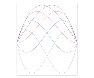
Figure 7. Plots of (a)  ${\tilde{R}_{Dc}}$, (b)
  ${a_c}$ and (c)
  ${c_c}$ versus m for different heterogeneity models of permeability: linear (black), quadratic (red) and exponential (blue).
Table 3. Critical values of  $({\tilde{R}_D},a,c)$ for various selected parametric values.

The variation of the corresponding critical wavenumber  ${a_c}$ is shown as a function of m in figure 7(b). For linear and quadratically varying permeability models,
  ${a_c}$ increases sharply at the beginning and then starts decreasing with increasing
  $|m|$ and
  $- m$, respectively. For the permeability model varying exponentially,
  ${a_c}$ increases initially then starts decreasing and again increases steadily for values of
  $|m|\ge 2.21$, and eventually attains the value
  ${a_c} = 0.5207|m|$ for sufficiently large values of
  $|m|$. Thus the size of the convection cell diminishes as
  $|m|$ takes larger values. The critical wave speed
  ${c_c}$ is found to increase steadily with decreasing
  $- m$ but decreases with decreasing m for both linear and exponential permeability models (figure 7c). In these cases, the sign of
  ${c_c}$ becomes negative when m is positive and vice versa but its modulus does not change. Thus cells move up the vertical porous slab when the solutions correspond to
  ${c_c} < 0$ and move down when
  ${c_c} > 0$. For a quadratic form of permeability,
  ${\pm} {c_c}$ exists for each value of
  $- m$, indicating wave disturbances travelling vertically both upward and downward with equal speed. This is because, if
  $c = {c_1} + i{c_2}$ is an eigenvalue of
  ${B^{ - 1}}A$ for a given value of
  $- m$ and the wavenumber
  $a$, then
  $c ={-} {c_1} + i{c_2}$ is also an eigenvalue of
  ${B^{ - 1}}A$ as
  ${\psi _b}$ is an even function of x.
8. Conclusions
An analysis of the stability of natural convection has been carried out for a vertical porous slab considering linear, quadratic and exponential heterogeneities of the permeability. The boundaries of the slab are impermeable and kept at constant but different temperatures. The stability eigenvalue problem has been formulated and solved numerically by employing the Chebyshev collocation method. The neutral stability condition and the critical Darcy–Rayleigh number for different heterogeneity models are determined. The suitable symmetries of the stability eigenvalue problem for linear and exponential models of heterogeneity have been established, allowing us to gather information on the regime  $m < 0$ from the results of
  $m > 0$. Some of the important results of this analysis can be outlined as follows.
(i) Gill's proof of stability, for the case of constant permeability, has been restated. It has been evidenced that this proof turns out to be ineffective if heterogeneity in permeability exists.
(ii) The heterogeneities of the permeability change the basic flow dramatically and also make the base flow unstable depending on the heterogeneity model as well as the variable permeability constant m. In the limit of vanishingly small m, the results for constant permeability are retrieved.
(iii) For quadratic form of heterogeneity, the base flow remains stable for all positive values of m and the instability occurs only for negative values of m.
(iv) For linear heterogeneity of the permeability, the value of
${\tilde{R}_{Dc}}$ decreases in the range $0.3754 \le |m|\le 0.99$ but it pinches upward slightly in a smaller range of $|m|> 0.99$, after which the flow remains unstable. A similar behaviour is noticed for the permeability varying quadratically but only for negative values of m.(v) For the exponentially varying permeability, the base flow becomes destabilized by manifesting itself as a minimum in the
$(m,{\tilde{R}_{Dc}})$-plane in a parametric space $0.5695 \le |m|\le 1.9$ and instead stabilizes for $|m|> 1.9$. Also, ${\tilde{R}_{Dc}}$ and ${a_c}$ attain asymptotic values $86.92|m|$ and $0.5207|m|$, respectively, at sufficiently large values of $|m|$.(vi) The instability sets in always via a travelling-wave mode for all heterogeneity models of the permeability.


Finally, considering the novelty of the present study, we believe that additional research is needed to better understand the stability of this class of basic states. In particular, the transition to absolute instability, the dynamics of spatial modes and the nonlinear development of the disturbances are possible tasks for future work. One of the most intriguing breakthroughs of this study is the introduction of a model for permeable/partially permeable boundary conditions. Also, one may extend the present problem by considering the time-dependent velocity term in the momentum equation and also horizontal heterogeneity in thermal conductivity.
Acknowledgements
We are indebted to three anonymous referees whose incisive comments have led to improvements in the original manuscript.
Funding
B.M.S. acknowledges financial support from the grant PESUIRF/Math/2020/11 provided by PES University, India.
Declaration of interests
The authors report no conflict of interest.
Data availability
The data that support the findings of this study are available within the article.
Appendix A
The Galerkin method has been employed alternatively to solve the resulting eigenvalue problem constituted by (4.3)–(4.5). Accordingly,  $\varPsi (x)$and
  $\varTheta (x)$ are expanded in a series of basis functions
 \begin{equation}\varPsi (x) = \sum\limits_{n = 0}^N {{a_n}{\xi _n}(x)} ,\quad \varTheta (x) = \sum\limits_{n = 0}^N {{b_n}{\xi _n}(x)} ,\end{equation}
where  ${a_n}$ and
  ${b_n}$ are constants and the basis functions
  ${\xi _n}(x )$ are represented in terms of Legendre polynomials
  ${P_n}(x)$ satisfying the boundary conditions in the form
 \begin{equation}{\xi _n}(x) = (1 - {x^2}){P_n}(x).\end{equation}
 Equation (A1a,b) is substituted back into (4.3) and (4.4), and the resulting momentum and heat transport equations are multiplied by  ${\xi _m}(x)$ and integrated by parts with respect to x between
  $- 1$ and
  $1$. This procedure gives two simultaneous algebraic equations governing the coefficients
  ${a_n}$ and
  ${b_n}$, which can be written in the matrix form
 \begin{equation} \boldsymbol{\mathsf{A}}\boldsymbol{\mathsf{X}} = c\boldsymbol{\mathsf{B}}\boldsymbol{\mathsf{X}},\end{equation}
where
 \begin{equation}\boldsymbol{\mathsf{A}} = \begin{pmatrix} {{C_{mn}}}&{{D_{mn}}}\\
{{E_{mn}}}&{{F_{mn}}} \end{pmatrix};\quad \boldsymbol{\mathsf{B}} = \begin{pmatrix} {{G_{mn}}}&{{H_{mn}}}\\
{{I_{mn}}}&{{J_{mn}}} \end{pmatrix};\quad \boldsymbol{\mathsf{X}} = \begin{pmatrix} {a_n}\\ {b_n} \end{pmatrix}.\end{equation}
\begin{equation}\boldsymbol{\mathsf{A}} = \begin{pmatrix} {{C_{mn}}}&{{D_{mn}}}\\
{{E_{mn}}}&{{F_{mn}}} \end{pmatrix};\quad \boldsymbol{\mathsf{B}} = \begin{pmatrix} {{G_{mn}}}&{{H_{mn}}}\\
{{I_{mn}}}&{{J_{mn}}} \end{pmatrix};\quad \boldsymbol{\mathsf{X}} = \begin{pmatrix} {a_n}\\ {b_n} \end{pmatrix}.\end{equation}
The coefficients  ${C_{mn}}$–
 ${J_{mn}}$ involve the inner products of the basis functions given by
 \begin{align}
{C_{mn}} &= \left\langle
{\dfrac{1}{{K(x)}}({\xi_m}{{\xi^{\prime\prime}}_n} +
{a^2}{\xi_m}{\xi_n})} \right\rangle - \left\langle
{\dfrac{{K^{\prime}(x)}}{{{{[K(x)]}^2}}}{\xi_m}{{\xi^{\prime}}_n}}
\right\rangle ,\nonumber\\
{D_{mn}} &= \dfrac{{{{\tilde{R}}_D}}}{b}\langle {\xi _m}{{\xi
^{\prime}}_n}\rangle ,\quad {E_{mn}} =
\dfrac{{ia}}{2}\langle {\xi _m}{\xi _n}\rangle ,\nonumber\\
{F_{mn}} &={-} ia\langle {{\psi ^{\prime}}_b}{\xi _m}{\xi
_n}\rangle + \langle {\xi _m}{{\xi ^{\prime\prime}}_n} +
{a^2}{\xi _m}{\xi _n}\rangle ,\quad {G_{mn}} \approx 0,\nonumber\\
{H_{mn}} &= 0,\quad {I_{mn}} = 0,\quad {J_{mn}} =
ia\langle {\xi _m}{\xi _n}\rangle ,
\end{align}
\begin{align}
{C_{mn}} &= \left\langle
{\dfrac{1}{{K(x)}}({\xi_m}{{\xi^{\prime\prime}}_n} +
{a^2}{\xi_m}{\xi_n})} \right\rangle - \left\langle
{\dfrac{{K^{\prime}(x)}}{{{{[K(x)]}^2}}}{\xi_m}{{\xi^{\prime}}_n}}
\right\rangle ,\nonumber\\
{D_{mn}} &= \dfrac{{{{\tilde{R}}_D}}}{b}\langle {\xi _m}{{\xi
^{\prime}}_n}\rangle ,\quad {E_{mn}} =
\dfrac{{ia}}{2}\langle {\xi _m}{\xi _n}\rangle ,\nonumber\\
{F_{mn}} &={-} ia\langle {{\psi ^{\prime}}_b}{\xi _m}{\xi
_n}\rangle + \langle {\xi _m}{{\xi ^{\prime\prime}}_n} +
{a^2}{\xi _m}{\xi _n}\rangle ,\quad {G_{mn}} \approx 0,\nonumber\\
{H_{mn}} &= 0,\quad {I_{mn}} = 0,\quad {J_{mn}} =
ia\langle {\xi _m}{\xi _n}\rangle ,
\end{align}
where the inner product is defined as  $\langle \cdots \rangle = \int_{ - 1}^1 {( \cdots )\,\textrm{d}\kern0.7pt x}$. Equation (A3) is solved numerically, as explained in § 6, to obtain the critical stability parameters.


