2. Formulation

The starting point of this investigation is the forced barotropic vorticity equation

(2.1)\begin{equation}\frac{{\partial {\nabla ^2}{\psi ^ \ast }}}{{\partial {t^\ast }}} + J({\psi ^\ast },{\nabla ^2}{\psi ^\ast }) + {\beta ^\ast }\frac{{\partial {\psi ^\ast }}}{{\partial {x^\ast }}} = {F^\ast },\end{equation}

where ${\psi ^\ast }$ is the streamfunction, associated with the velocity field $({u^\ast },{v^\ast }) = ( - \partial {\psi ^\ast }/\partial {y^\ast },\partial {\psi ^\ast }/\partial {x^\ast })$, and J is the Jacobian. The term ${F^\ast }$ represents external forcing, which maintains the time-dependent basic state (1.2). To reduce the number of controlling parameters, the system is non-dimensionalized using ${({\bar{l}^\ast })^{ - 1}}$ as the unit of length, ${({\bar{\omega }^\ast })^{ - 1}}$ as the unit of time and ${\bar{\omega }^\ast }{({\bar{l}^\ast })^{ - 2}}$ as the unit of streamfunction. After non-dimensionalization, the vorticity equation reduces to

(2.2)\begin{equation}\frac{{\partial {\nabla ^2}\psi }}{{\partial t}} + J(\psi ,{\nabla ^2}\psi ) + \beta \frac{{\partial \psi }}{{\partial x}} = F,\end{equation}

where $\beta = {\beta ^\ast }/{\bar{\omega }^\ast }{\bar{l}^\ast }$, and the basic state becomes

(2.3)\begin{equation}\bar{u} = (A + B\cos (t))\sin (y),\end{equation}

where $(A,B) = ({\bar{l}^\ast }/{\bar{\omega }^\ast })({A^\ast },{B^\ast })$. The stability analysis of this system commences by linearizing (2.2) about the basic state (2.3) to obtain

(2.4)\begin{equation}\partial {\nabla ^2}\psi ^{\prime}/\partial t + J(\bar{\psi },{\nabla ^2}\psi ^{\prime}) + J(\psi ^{\prime},{\nabla ^2}\bar{\psi }) + \beta \frac{{\partial \psi ^{\prime}}}{{\partial x}} = 0,\end{equation}

where

(2.5)\begin{equation}\bar{\psi } = (A + B\cos (t))\cos (y).\end{equation}

To investigate the interaction of pattern (2.5) with much larger scales of motion $({L_x},{L_y} \gg 1)$, we introduce a small parameter

(2.6)\begin{equation}\varepsilon = \frac{{2{\rm \pi} }}{{{L_y}}},\end{equation}

which represents the ratio of the dominant meridional wavelengths of the large-scale perturbation and the basic state. This parameter is used to define the new set of spatial and temporal scales $(X,Y,T)$, which are related to the original variables as follows:

(2.7a–c)\begin{equation}X = {\varepsilon ^2}x,\quad Y = \varepsilon y,\quad T = {\varepsilon ^2}t.\end{equation}

While the asymptotic ordering of the large-scale meridional variable (Y) follows directly from the definition of $\varepsilon $ in (2.6), the identification of relevant large zonal scales is less trivial. We anticipate that the periodic variation in the basic state, which occurs on the O(1) time scale, could resonate with free Rossby waves and induce their amplification. The dispersion relation of large-scale barotropic Rossby waves is

(2.8)\begin{equation}\omega ={-} \frac{{\beta k}}{{{k^2} + {l^2}}},\end{equation}

where $\omega $ is the frequency and $(k,l)$ are the wavenumbers. Since by definition $l = \varepsilon $, O(1) frequencies are realized for $k\sim {\varepsilon ^2}$, which suggests scaling (2.7a) of the large-scale zonal variable X. The time scale T represents the relatively slow growth of large-scale patterns.

In the present configuration, we expect to find x-invariant solutions. This assumption can be rationalized by recalling that the basic state (2.5) does not vary in the zonal direction. Hence, its interaction with large-scale patterns is expected to generate secondary patterns that are also devoid of small-scale variability in x, and solutions of the governing equation (2.4) are sought in five-dimensional space as

(2.9)\begin{equation}\psi ^{\prime} = \psi ^{\prime}(X,y,Y,t,T).\end{equation}

Thus, the derivatives in the governing equation (2.4) are replaced using

(2.10a–c)\begin{equation}\frac{\partial }{{\partial x}} \to {\varepsilon ^2}\frac{\partial }{{\partial X}}\textrm{ },\quad \frac{\partial }{{\partial y}} \to \frac{\partial }{{\partial y}} + \varepsilon \frac{\partial }{{\partial Y}},\quad \frac{\partial }{{\partial t}} \to \frac{\partial }{{\partial t}} + {\varepsilon ^2}\frac{\partial }{{\partial T}},\end{equation}

and both sets of variables are treated as independent variables. As a result, (2.10a–c) transforms (2.4) into

(2.11) \begin{align} &\frac{{\partial \varsigma ^{\prime}}}{{\partial t}} + {\varepsilon ^2}\frac{{\partial \varsigma ^{\prime}}}{{\partial T}} + {\varepsilon ^2}{J_{Xy}}(\bar{\psi },\varsigma ^{\prime}) + {\varepsilon ^2}{J_{Xy}}(\psi ^{\prime},\bar{\varsigma }) + {\varepsilon ^3}{J_{XY}}(\bar{\psi },\varsigma ^{\prime})\nonumber\\ &\quad + {\varepsilon ^3}{J_{XY}}(\psi ^{\prime},\bar{\varsigma }) + \beta {\varepsilon ^2}\frac{{\partial \psi ^{\prime}}}{{\partial X}} = 0,\end{align}

where ${J_{Xy}}$ and ${J_{XY}}$ are the Jacobians in $(X,y)$ and $(X,Y)$, $\bar{\varsigma } = {\nabla ^2}\bar{\psi }$ and $\varsigma ^{\prime} = {\nabla ^2}\psi ^{\prime}$ are the basic and perturbation vorticities and

(2.12)\begin{equation}{\nabla ^2} \equiv {\varepsilon ^4}\frac{{{\partial ^2}}}{{\partial {X^2}}} + \frac{{{\partial ^2}}}{{\partial {y^2}}} + 2\varepsilon \frac{{{\partial ^2}}}{{\partial y\,\partial Y}} + {\varepsilon ^2}\frac{{{\partial ^2}}}{{\partial {Y^2}}}.\end{equation}

To explore the weak interaction between large-scale patterns and the basic flow, we consider the evolution of the plane wave

(2.13)\begin{equation}{\psi _w} = {\hat{\psi }_w}{\rm exp} \{ \textrm{i}(KX + Y - {\omega _o}t - {\omega _2}T)\} ,\end{equation}

where $K = k{\varepsilon ^{ - 2}} = O(1)$ is the rescaled large-scale zonal wavenumber, ${\omega _0}$ is the zero-order frequency and ${\omega _2}$ is the correction induced by the weak interaction with the basic state (2.5). The imaginary component of the perturbation frequency measures the wave growth rate,

(2.14)\begin{equation}\lambda = {\varepsilon ^2}{\rm Im}({\omega _2}).\end{equation}

In the absence of the interaction with the basic state, the plane wave (2.13) would oscillate at the frequency

(2.15)\begin{equation}\omega ={-} \frac{{\beta K}}{{{K^2}{\varepsilon ^2} + 1}},\end{equation}

and the full-period resonance $(\omega = 1)$ for $\varepsilon \to 0$ is expected to occur at $K \approx{-} {\beta ^{ - 1}}$. However, to properly account for the wave interaction with the basic state, it becomes critical to explore a continuous range of values in the vicinity of the leading-order resonant wavenumber

(2.16)\begin{equation}K ={-} {\beta ^{ - 1}}(1 + \delta {\varepsilon ^2}),\end{equation}

where $\delta $ is an O(1) quantity. The leading-order frequency of the plane wave is assumed to match that of the basic state,

(2.17)\begin{equation}{\omega _0} = 1.\end{equation}

Another step that proved to be instrumental in reducing the number of controlling parameters is the renormalization of the basic state amplitude using

(2.18a,b)\begin{equation}A = {A_n}\beta ,\quad B = {B_n}\beta .\end{equation}

The solution of the governing equations is now sought in terms of a power series in $\varepsilon \ll 1$,

(2.19)\begin{equation}\psi ^{\prime} = {\psi _0}(X,y,Y,t,T) + \varepsilon {\psi _1}(X,y,Y,t,T) + {\varepsilon ^2}{\psi _2}(X,y,Y,t,T) + \cdots .\end{equation}

We substitute (2.19) into (2.11), collect terms of the same order in $\varepsilon $ and sequentially solve the set of balances realized at each level in the expansion until an explicit expression for the growth rate (2.14) is obtained. The necessary solvability condition for this system is that the small-scale average of (2.11) is zero. This requirement applies to all orders in the expansion. However, as will be seen shortly, it is trivially satisfied at orders from the zeroth through the third. At the fourth order, however, the averaging over $(y,t)$ yields the evolutionary equation for the large-scale component, which makes it possible to evaluate the growth rates of unstable modes. This procedure is illustrated first using the relatively simple case of a purely oscillatory basic state $(A = 0)$ and then generalized (§ 4) to include a finite steady component $(A \ne 0)$.

3. Oscillatory basic state $(A = 0)$

3.1. Multiscale expansion

The expansion opens with the large-scale plane wave (2.13), which is included in the leading-order component ${\psi _0}$. It automatically satisfies the O(1) and $O(\varepsilon )$ balances of the governing equation (2.11). However, we note that these balances are also satisfied by adding to ${\psi _w}$ any slowly varying function ${g_0}$ of the form

(3.1)\begin{equation}{g_0} = {\hat{\psi }_w}{C_0}\cos (y){\rm exp} \{ \textrm{i}(KX + Y - {\omega _2}T)\} .\end{equation}

Thus, we seek the solution for the O(1) component of $\psi ^{\prime}$ by assuming

(3.2)\begin{equation}{\psi _0} = {\psi _w} + {g_0},\end{equation}

with the expectation that the coefficient ${C_0}$ will be determined at a higher-order level in the expansion. Similarly, for the $O(\varepsilon )$ component of $\psi ^{\prime}$ we consider the function

(3.3)\begin{equation}{\psi _1} = {\hat{\psi }_w}{C_1}\sin (y){\rm exp} \{ \textrm{i}(KX + Y - {\omega _2}T)\} ,\end{equation}

and its inclusion also satisfies the $O(\varepsilon )$ balance.

At the second order, we consider the solution of the form

(3.4)\begin{equation}{\psi _2} = {\psi _w}(C_2^{(c)}\cos (t) + C_2^{(s)}\sin (t))\cos (y).\end{equation}

The $O({\varepsilon ^2})$ balance is satisfied as long as

(3.5)\begin{equation}{C_0} = \frac{1}{2}\frac{{{B_n}}}{{1 - {\omega _2}}}\end{equation}

and

(3.6)\begin{equation}C_2^{(c)} ={-} \frac{{{B_n}}}{2} - {\rm i}C_2^{(s)}.\end{equation}

The $O({\varepsilon ^3})$ balance is characterized by the appearance of terms that are proportional to $\cos (2t),$ $\sin (2t),$ $\cos (2y)$ and $\sin (2y)$. This feature demands that we seek the third-order component by assuming a more general structure

(3.7) \begin{align}{\psi _3} &= {\psi _w}\sin (y)(C_3^{(c)}\cos (t) + C_3^{(s)}\sin (t)) + {\psi _w}\sin (2y)(C_3^{(2c)}\cos (2t)\nonumber\\ &\quad + C_3^{(2s)}\sin (2t) + C_3^{(0)}).\end{align}

The $O({\varepsilon ^3})$ balance is satisfied as long as

(3.8)\begin{equation}{C_1} = \frac{{{\rm i}{B_n}{\omega _2}}}{{{{({\omega _2} - 1)}^2}}}\end{equation}

and

(3.9a–d)\begin{align}C_3^{(c)} = {\rm i}({B_n} - C_3^{(s)}),\quad C_3^{(2c)} = \frac{{{\rm i}B_n^2}}{{16({\omega _2} - 1)}},\quad C_3^{(2s)} = \frac{{B_n^2}}{{16(1 - {\omega _2})}},\quad C_3^{(2c)} = \frac{{{\rm i}B_n^2}}{{16(1 - {\omega _2})}}.\end{align}

The sought-after expression for the growth rate is obtained as a solvability condition, by averaging the $O({\varepsilon ^4})$ balance in small-scale variables $(y,t)$:

(3.10)\begin{equation}{\beta ^2}(3B_n^2{\omega _2} + 8\delta \omega _2^2 - 8\omega _2^3 + B_n^2 - 16\delta {\omega _2} + 16\omega _2^2 + 8\delta - 8{\omega _2}) = 8{({\omega _2} - 1)^2}.\end{equation}

For given $\beta $ and ${B_n}$, (3.10) implicitly determines ${\omega _2}(\delta )$. Thus, the identification of the most rapidly amplifying mode requires maximizing ${\rm Im}({\omega _2})$ as a function of $\delta $. This is accomplished by separating the complex frequency ${\omega _2}$ into real and imaginary components:

(3.11)\begin{equation}{\omega _2}(\delta ) = a(\delta ) + {\rm i}b(\delta ),\end{equation}

where a and b are real quantities. We also isolate real and imaginary components of (3.10), resulting in

(3.12) \begin{align}\begin{aligned} & ( - 8 + (8\delta + 16){\beta ^2})a{(\delta )^2} + (24{\beta ^2}b{(\delta )^2} + 16 + (3B_n^2 - 16\delta - 8){\beta ^2})a(\delta )\nonumber\\ & \quad - 8{\beta ^2}a{(\delta )^3} + (8 + ( - 8\delta - 16){\beta ^2})b{(\delta )^2} - 8 + (B_n^2 + 8\delta ){\beta ^2} = 0 \end{aligned}\end{align}

and

(3.13)\begin{align}( - 16 + (16\delta + 32){\beta ^2})a(\delta ) - 24{\beta ^2}a{(\delta )^2} + 8{\beta ^2}b{(\delta )^2} + 16 + (3B_n^2 - 16\delta - 8){\beta ^2} = 0.\end{align}

To determine the maximum of $b(\delta )$, we differentiate (3.12) and (3.13) with respect to $\delta $ and simplify the result by insisting that $(\partial /\partial \delta )b(\delta ) = 0$, which yields

(3.14) \begin{align}\begin{aligned} & 8{\beta ^2}{a^2} - 24{\beta ^2}{a^2}c + 2( - 8 + (8\delta + 16){\beta ^2})ac - 16{\beta ^2}a\\ & \quad + (24{\beta^2}{b^2} + 16 + (3B_n^2 - 16\delta - 8){\beta ^2})c - 8{\beta ^2}{b^2} + 8{\beta ^2} = 0 \end{aligned}\end{align}

and

(3.15)\begin{equation}16{\beta ^2}a - 48{\beta ^2}ac + ( - 16 + (16\delta + 32){\beta ^2})c - 16{\beta ^2} = 0,\end{equation}

where $c \equiv (\partial /\partial \delta )a(\delta )$.

The system of algebraic equations (3.12)–(3.15) can now be solved for any given $(\beta ,{B_n})$. First, we solve (3.15) for $\delta $ to get

(3.16) \begin{equation}\delta = \frac{{{\beta ^2}(3ac - a - 2c + 1) + c}}{{{\beta ^2}c}},\end{equation}

and then we use (3.16) to eliminate $\delta $ in (3.12)–(3.14) in favour of $(a,b,c)$, obtaining

(3.17) \begin{align} \left. {\begin{array}{c@{}} {(3B_n^2 + 24{a^2} + 8{b^2} - 48a + 24)c - 16{{(a - 1)}^2} = 0},\\ {(16c - 8){a^3} - (48c - 24){a^2} + (3B_n^2c + 8{b^2} + 48c - 24)a + B_n^2c - 8{b^2} - 16c + 8 = 0},\\ {(3B_n^2 + 24{a^2} + 24{b^2} - 48a + 24)c - 8{a^2} - 8{b^2} + 16a - 8 = 0.} \end{array}} \right\}\end{align}

The elimination of $\delta $ produces an unexpected simplification. Remarkably, system (3.17) is independent of $\beta $, which implies that the solution is fully determined by the normalized amplitude of the basic flow ${B_n}$. The resulting relation $b({B_n})$ is shown in figure 1. Since the growth rate equations (3.17) are invariant with respect to the change in the sign of ${B_n}$, the results are presented only for ${B_n} \ge 0$. Figure 1 reveals the monotonic increase in the rescaled growth rate (b) with the normalized amplitude $|{B_n}|$. An even more significant finding is the unconditional instability $(b > 0)$ of time-dependent oscillating zonal flows. This instability is realized even when the system is stable according to the Rayleigh–Kuo criterion (1.3), which in the present configuration $(A = 0)$ reduces to $|{B_n}|< 1$.

Figure 1. The rescaled growth rate, b, is plotted as a function of the parameter ${B_n}$, which controls the strength of the time-dependent component of the basic state, for the oscillatory model $(A = 0)$.

The foregoing multiscale analysis indicates that the instability of time-dependent flows can be attributed to resonant triad interaction. The primary plane wave operating on frequencies that are close to that of the basic state (i.e. ${\propto} \cos (kx + ly - t - {\varepsilon ^2}{\omega _2}t)$) interacts with the basic state $\cos (y)\cos (t)$ and produces, among other harmonics, the secondary mode proportional to $\sin (kx + ly + y - {\varepsilon ^2}{\omega _2}t)$. This secondary mode itself interacts with the basic state and produces a component proportional to the primary mode. As a result, the primary mode amplifies. The multiscale model formalizes this interaction by identifying balances that arise at each order in $\varepsilon $ and thereby explaining the chain of events leading to the instability.

3.2. Validation

At this stage, the multiscale analysis is complete and we can revert to the original variables using (2.6), (2.7a–c), (2.14) and (2.16), which yields the maximal growth rate

(3.18)\begin{equation}{\lambda _{lin\;ms}} = \frac{{4{{\rm \pi} ^2}}}{{L_y^2}}b({B_n})\end{equation}

and a corresponding zonal wavenumber of

(3.19)\begin{equation}{k_{max}} ={-} \frac{{4{{\rm \pi} ^2}}}{{\beta L_y^2}}\left( {1 + \frac{{4{{\rm \pi} ^2}}}{{L_y^2}}\delta (\beta ,{B_n})} \right).\end{equation}

To assess the accuracy of the foregoing asymptotic $(\varepsilon \to 0)$ model (3.18), we now attempt to evaluate the growth rate numerically. This objective is accomplished by employing the zonally truncated model, in which

(3.20)\begin{equation}\psi ^{\prime} = {\hat{\psi }_c}(y)\cos (kx) + {\hat{\psi }_s}(y)\sin (kx).\end{equation}

We substitute (3.20) into the linearized vorticity equation (2.4) and isolate terms proportional to $\cos (kx)$ and $\sin (kx)$, resulting in

(3.21) \begin{equation}\frac{\partial }{{\partial t}}\left( \begin{array}{@{}l@{}} \dfrac{{{\partial^2}{{\hat{\psi }}_c}}}{{\partial {y^2}}} - {k^2}{{\hat{\psi }}_c}\\ \dfrac{{{\partial^2}{{\hat{\psi }}_s}}}{{\partial {y^2}}} - {k^2}{{\hat{\psi }}_s} \end{array} \right) = \boldsymbol{L}\left(\begin{array}{@{}l@{}} {{\hat{\psi }}_c}\\ {{\hat{\psi }}_s} \end{array} \right),\end{equation}

where $\boldsymbol{L}$ is a linear differential operator with time-dependent coefficients. The truncated system (3.21) was integrated in time using the Fourier spectral method (e.g. Radko Reference Radko2014), which assumes periodic boundary conditions for $({\hat{\psi }_c},{\hat{\psi }_s})$ at $y = 0,{\varGamma _y}$ and is based on the fourth-order Runge–Kutta time-stepping algorithm. In each of the following simulations, the extent of the computational interval $({\varGamma _y})$ is assigned the value of the y-wavelength of the unstable mode, ${L_y} = 2{\rm \pi} /\varepsilon $. We discretize the system using 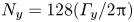${N_y} = 128({\varGamma _y}/2{\rm \pi} )$ grid points in y and initiate simulations by the random distribution of $({\hat{\psi }_c},{\hat{\psi }_s})$. The growth rate is evaluated using the temporal record of the mean perturbation kinetic energy

(3.22)\begin{equation}e(t) = {[{\textstyle{1 \over 2}}|\boldsymbol{\nabla }\psi ^{\prime}{|^2}]_{xy}}, \end{equation}

where ${[ \cdots ]_{xy}}$ denotes the spatial average. A representative calculation of this type is shown in figure 2(a), which was performed for ${B_n} = 0.5$, $\beta = 1$, $\varepsilon = 0.2$, ${\varGamma _y} = 10{\rm \pi} $ and $k ={-} 0.0434$ – the latter was determined using (3.19). After the initial adjustment period, the perturbation starts to grow in a nearly exponential manner. The best linear fit to ${\textstyle{1 \over 2}}\ln (e)$ over the second half of the simulation 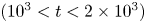$({10^3} < t < 2 \times {10^3})$ yields the numerical estimate of the growth rate, ${\lambda _{lin\;k}} = 1.\textrm{29} \times \textrm{1}{\textrm{0}^{ - 2}}$.

Figure 2. (a) The temporal record of ${\textstyle{1 \over 2}}\ln (e)$ obtained by the numerical integration of the truncated system (3.21) for ${B_n} = 0.5$, $\beta = 1$, ${L_y} = 10{\rm \pi} $ and $|k|= 0.0434$. The numerical estimate of the growth rate $({\lambda _{num}} = 1.29 \times {10^{ - 2}})$ is determined from the best linear fit to this record over the second half of the integration interval. (b) The numerical estimates of the growth rate are plotted on the logarithmic scale as a function of $\varepsilon = 2{\rm \pi} /{L_y}$ for $\beta = 1$ (plus signs) and for $\beta = 10$ (circles). The asymptotic prediction is indicated by the solid line.

A series of calculations analogous to those in figure 2(a) was performed for ${\varGamma _y} = {L_y} = 2{\rm \pi} n$, where $n = 3,4, \ldots ,10$. The resulting values of ${\lambda _{lin\;k}}$ are plotted as a function of $\varepsilon = 2{\rm \pi} /{L_y} = 1/n$ in logarithmic coordinates in figure 2(b), along with the theoretical prediction (3.18). These calculations indicate that as $\varepsilon $ decreases, the numerical and asymptotic results systematically converge. For $\varepsilon = 0.1$, these predictions differ by a mere 4 %. Such agreement between the numerics and theory lends credence to the multiscale instability model.

An interesting property of BTSI revealed by the multiscale model is that the growth rate is uniquely determined by ${B_n}$. This surprising finding prompts the question of whether such invariance with respect to $\beta $ is an exclusive feature of the long-wavelength approximation used in the multiscale theory. To address this possibility, a set of numerical calculations was performed with $\beta = 10$, which are also shown in figure 2(b). As expected, the growth rates for the different $\beta $ are close for small $\varepsilon $, as both series approach the same asymptotic long-wavelength pattern. However, they visibly diverge for O(1) wavenumbers.

4. Effects of a finite steady component $(A \ne 0)$

The foregoing multiscale model is now generalized by considering a basic state which contains a finite steady component. While this extension represents a significant step towards realism, particularly in the context of geophysical applications (§ 1), it also leads to substantial technical difficulties. The development of the multiscale theory generally follows that in § 3. However, in the special case of $A = 0$, a consistent asymptotic solution was obtained which involves only the two lowest harmonics in y. The principal complication in the finite-A case is caused by the excitation of an infinite series of Fourier components in y. Therefore, the earlier theory was modified using the Galerkin projection method, in which the solution for $\psi ^{\prime}$ is constructed using the N lowest harmonics in y. To find an appropriate solution, we insist that the substitution of the truncated series into the governing equation not project onto these low harmonics in y. The increase in N makes it possible to determine solutions with any desired accuracy.

While the leading-order streamfunction component is still given by (3.1) and (3.2), the first-order solution takes the form of

(4.1)\begin{equation}{\psi _1} = {\hat{\psi }_w}\sum\limits_{m = 1}^N {C_1^{(m)}\sin (my){\rm exp}\{ \textrm{i}(KX + Y - {\omega _2}T)\} } .\end{equation}

The $O({\varepsilon ^2})$ and $O({\varepsilon ^3})$ balances of the governing equation demand that the second- and third-order components of the streamfunction be represented by the following patterns:

(4.2)\begin{equation}{\psi _2} = {\psi _w}(C_2^{(c)}\cos (t) + C_2^{(s)}\sin (t) + C_2^{(0)})\cos (y)\end{equation}

and

(4.3) \begin{align}{\psi _3} &= {\psi _w}(C_3^{(c)}\cos (t) + C_3^{(s)}\sin (t)) \nonumber\\ &\quad + {\psi _w}\sum\limits_{m = 1}^N {\sin (my)} (C_3^{(2c)(m)}\cos (2t)+ C_3^{(2s)(m)}\sin (2t) + C_3^{(0)(m)}).\end{align}

The coefficients C in (4.1)–(4.3) are determined by the Galerkin projection, and the solvability condition at $O({\varepsilon ^4})$ yields the growth rate. The growth rate calculations have been performed for $N = 2, \ldots ,5$. Offhand, one would expect these solutions to be accurate only for a large number of harmonics. Fortunately, our model is characterized by the remarkably rapid convergence of the solutions with increasing N. For instance, the relative difference between the growth rates evaluated for $({A_n},{B_n},\beta ) = (0.5,0.25,1)$ using $N = 3$ and $N = 4$ is $3.54 \times {10^{ - 5}}$. The difference between the $N = 4$ and $N = 5$ models is only $1.47 \times {10^{ - 5}}$. Thus, for most intents and purposes, it is safe to assume that the three-mode approximation fully represents the system dynamics. The coefficients of the streamfunction components in (4.1)–(4.3) and the resulting growth rate equation for $N = 3$ are listed in Appendix A.

As previously (§ 3), we find that the rescaled maximal growth rate (b) is uniquely determined by the normalized magnitude of the basic flow, measured by ${A_n}$ and ${B_n}$. The resulting relation $b = b({A_n},{B_n})$ is shown in figure 3. Since the growth rate is invariant with respect to the change in sign of ${A_n}$ and ${B_n}$, the results are presented only for ${A_n} \ge 0$ and ${B_n} \ge 0$ without loss of generality. While growth rate pattern in figure 3 was obtained for $N = 3$, it is visually indistinguishable from its counterparts for $N = 4$ and $N = 5$. A notable feature of this calculation is the unconditional linear instability of the system. Particularly intriguing is the instability in the regime where the flow is stable according to the Rayleigh–Kuo criterion (1.3). When expressed in terms of ${A_n}$ and ${B_n}$, this criterion reduces to

(4.4)\begin{equation}|{A_n}|+ |{B_n}|< 1.\end{equation}

Figure 3. The rescaled growth rate, b, is plotted as a function of the parameters ${A_n}$ and ${B_n}$, which control the strength of the basic current. The region below the dashed line represents the part of parameter space where the flow is stable according to the Rayleigh–Kuo criterion.

The corresponding region in the $({A_n},{B_n})$ parameter space is located below the dashed line in figure 3. Given the relatively high growth rates in this region, we anticipate that time-dependent Rayleigh-stable flows exhibit vigorous instability and transition to turbulence at fully nonlinear stages. This expectation will be confirmed shortly (§ 5) by direct numerical simulations.

At this point, we revert to the original (small-scale) variables. The growth rate takes the form of

(4.5)\begin{equation}{\lambda _{lin\;ms}} = {\varepsilon ^2}b({A_n},{B_n}) = \frac{{4{{\rm \pi} ^2}}}{{L_y^2}}b({A_n},{B_n}),\end{equation}

and the corresponding zonal wavenumber is

(4.6)\begin{equation}{k_{max}} ={-} {\beta ^{ - 1}}{\varepsilon ^2}(1 + {\varepsilon ^2}\delta ({A_n},{B_n},\beta )) ={-} {\beta ^{ - 1}}\frac{{4{{\rm \pi} ^2}}}{{L_y^2}}\left( {1 + \frac{{4{{\rm \pi} ^2}}}{{L_y^2}}\delta ({A_n},{B_n},\beta )} \right).\end{equation}

The asymptotic result (4.5) has been validated by the truncated numerical model (3.21). Figure 4 presents a series of numerical integrations for $({A_n},{B_n},\beta ) = (0.5,0.25,1)$ and various values of ${L_y}$, revealing the convergence of the numerical and asymptotic estimates of $\lambda $ with decreasing $\varepsilon = 2{\rm \pi} /{L_y}$.

Figure 4. The growth rates are determined by the numerical integration of the truncated system (3.21) for $({A_n},{B_n},\beta ) = (0.5,0.25,1)$. These numerical estimates, indicated by the plus signs, are plotted on the logarithmic scale as a function of $\varepsilon = 2{\rm \pi} /{L_y}$ along with the corresponding asymptotic prediction (solid line).

Another interesting property of BTSI is the contrast between the strong dependence of the rescaled growth rates (b) on ${B_n}$ and their very weak dependence on ${A_n}$. This feature makes it possible to formulate simple empirical relations for the growth rate as a function of ${B_n}$ only. For instance, the pattern in figure 3 can be approximated by the power-law relation

(4.7a–c)\begin{equation}{b_{fit}} = DB_n^\alpha ,\quad D = \textrm{0}\textrm{.5768},\quad \alpha = \textrm{0}\textrm{.6137,}\end{equation}

with a relative root-mean-square error of only 5.76 %. For utilitarian purposes, it might prove useful to express this result in terms of dimensional quantities as

(4.8)\begin{equation}{\lambda ^\ast } = \frac{{4{{\rm \pi} ^2}{{\bar{\omega }}^\ast }}}{{{{(L_y^\ast {{\bar{l}}^\ast })}^2}}}D{\left( {\frac{{{B^\ast }{{{\bar{l}}^\ast }}{^2}}}{{{\beta^\ast }}}} \right)^\alpha }.\end{equation}

This empirical relation illustrates that the growth rate increases with the increasing frequency of oscillations $({\bar{\omega }^\ast })$ and with decreasing ${\beta ^\ast }$. The latter observation may seem counterintuitive, considering that the instability mechanism is the resonant forcing of the Rossby waves that requires the beta-effect. Such a conundrum indicates that the multiscale model in its present form, which from the outset assumes $\beta = O(1)$, cannot properly represent the singular limit of $\beta \to 0$. This view is supported by the analysis of the non-rotating $(\beta = 0)$ case, where the inviscid Kolmogorov flow with $A = 0$ is always stable (Frenkel Reference Frenkel1991).

5. Direct numerical simulations

The foregoing linear analysis reveals the ubiquity of non-traditional barotropic instabilities of time-dependent shear flows, motivating efforts to explore their nonlinear development. This objective is addressed by performing a series of numerical simulations of the governing equation (2.2) using the Fourier-based spectral model (e.g. Sutyrin & Radko Reference Sutyrin and Radko2019). The model is de-aliased using the zero-padding algorithm and employs the fourth-order Runge–Kutta time-stepping scheme. To control the numerical stability of the code, (2.2) is augmented by the frictional term with a minimal viscosity of $\nu = 2 \times {10^{ - 4}}$. The result is then expressed in terms of the perturbation streamfunction as follows:

(5.1)\begin{equation}\frac{{\partial {\nabla ^2}\psi ^{\prime}}}{{\partial t}} + J(\psi ^{\prime},{\nabla ^2}\bar{\psi }) + J(\bar{\psi },{\nabla ^2}\psi ^{\prime}) + J(\psi ^{\prime},{\nabla ^2}\psi ^{\prime}) + \beta \frac{{\partial \psi ^{\prime}}}{{\partial x}} = \nu {\nabla ^4}\psi ^{\prime}.\end{equation}

The integrations of (5.1) were performed on a doubly periodic domain of size $({\varGamma _x},{\varGamma _y}) = (24{\rm \pi} ,12{\rm \pi} )$, which was resolved by $({N_x},{N_y}) = (4096,2048)$ Fourier modes. The simulations were initialized by a small-amplitude random $\psi ^{\prime}(x,y)$ distribution. A typical experiment designed in this manner is shown in figures 5 and 6, where we present the perturbation streamfunction $(\psi ^{\prime})$ and vorticity $(\varsigma ^{\prime} = {\nabla ^2}\psi ^{\prime})$ fields, respectively. The governing parameters for this system $({A_n} = 0.5,\;{B_n} = 0.25)$ place it in the category of Rayleigh-stable flows, and therefore the amplification of perturbations is attributed exclusively to the BTSI dynamics.

Figure 5. Direct numerical integrations of (5.1). The instantaneous perturbation streamfunction $(\psi ^{\prime})$ fields are shown at various times in (a–c). The experimental parameters are ${A_n} = 0.5$, ${B_n} = 0.25$, $\beta = 1$, ${\varGamma _x} = 24{\rm \pi} $, ${\varGamma _y} = 12{\rm \pi} $, ${N_x} = 4096$ and ${N_y} = 2048$.

Figure 6. The same as figure 5 but for the vorticity perturbation $\varsigma ^{\prime} = {\nabla ^2}\psi ^{\prime}$.

The evolution of the flow field in this simulation is representative of most laminar-turbulent transition problems. After the adjustment period $(t\mathrm{\ \mathbin{\lower.3ex\hbox{$\buildrel< \over {\smash{\scriptstyle\sim}\vphantom{_x}}$}}\ }200)$, unstable modes emerge from the random initial perturbation field and start to amplify (figures 5a and 6a). These modes nonlinearly equilibrate by $t\sim 500$ (figures 5b and 6b), and their subsequent evolution is characterized by the development of chaotic and disorganized patterns. Finally, after $t\sim 700$, the flow field starts to exhibit a wide range of spatial scales (figures 5c and 6c), which is an expected manifestation of fully developed turbulence. The streamfunction field (figure 5c) is dominated by large-scale structures, the lateral extent of which is comparable to the size of the computational domain. However, the corresponding vorticity field (figure 6c) reveals the presence of small-scale patterns directly controlled by explicit friction.

Figure 7 illustrates the temporal variability of the spatially averaged perturbation energy (3.22) and enstrophy

(5.2)\begin{equation}r = {[{\textstyle{1 \over 2}}{(\varsigma ^{\prime})^2}]_{xy}},\end{equation}

diagnosed from four simulations with various $({A_n},{B_n})$. The experiments presented were performed with ${A_n} = 0.5$, ${B_n} = 0.25$ (EXP1); ${A_n} = 0.25$, ${B_n} = 0.25$ (EXP2); ${A_n} = 0$, ${B_n} = 0.5$ (EXP3); and ${A_n} = 0.25$, ${B_n} = 0.5$ (EXP4). The time series of energy (figure 7a) and enstrophy (figure 7b) are characterized by nearly exponential initial growth and subsequent equilibration at finite statistically steady levels. The system behaviour is sensitive to the values of ${B_n}$. The growth rates and the equilibrium levels of e and r substantially increase when the magnitude of the time-dependent component is raised from ${B_n} = 0.25$ (EXP1 and EXP2) to ${B_n} = 0.5$ (EXP3 and EXP4).

Figure 7. The temporal records of the spatially averaged perturbation energy (e) and enstrophy (r) are plotted on the logarithmic scale. The experiments performed with $({A_n},{B_n}) =\ $$(0.5,0.25)$, $(0.25,0.25)$, $(0,0.5)$ and $(0.25,0.5)$ are shown in black, blue, red and green, respectively. In all simulations $\beta = 1$.

On the other hand, the influence of the steady component $({A_n})$ on the system dynamics is rather limited. The time series of the energy and enstrophy generated for the same ${B_n}$ but different values of ${A_n}$ are generally similar. Such a strong (weak) dependence of fully nonlinear solutions in figure 7 on ${B_n}({A_n})$ is consistent with the properties of linear long-wavelength solutions in § 4 (e.g. figure 3).

To ensure the mutual consistency of simulations in figure 7 and the foregoing (§§ 3 and 4) linear analyses, we find it instructive to compare the growth rates obtained using various methods (table 1). The growth rates in simulations $({\lambda _{DNS}})$ were evaluated over the intervals of nearly exponential growth, defined by requiring ${10^{ - 8}} < e < {10^{ - 1}}$. In each experiment, ${\lambda _{DNS}}$ was determined from the best linear fit to ${\textstyle{1 \over 2}}\ln (e)$ over this interval. The linear growth rates were computed using two other methods: (i) integration of the linearized single-mode equations $({\lambda _{lin\;k}})$ using the technique described in § 3.2; and (ii) extrapolation of the multiscale model $({\lambda _{lin\;ms}})$. The advantage of the single-mode truncation model is that it makes no assumptions regarding the wavelength of unstable perturbations, whereas the multiscale theory only represents the long-wavelength limit.

Table 1. The growth rates realized in the numerical simulations $({\lambda _{DNS}})$ are listed along with the corresponding estimates based on the linear single-mode model $({\lambda _{lin\;k}})$ and the multiscale theory $({\lambda _{lin\;ms}})$.

The growth rate in the single-mode model was computed using the vertical scale of ${\varGamma _y} = 12{\rm \pi} $ and $k ={-} 2{\rm \pi} j/{\varGamma _x}$, where $j = 1,2, \ldots $ and ${\varGamma _x} = 24{\rm \pi} $, thus exactly matching the dimensions of the computational domain used in simulations. The growth rates obtained for various wavenumbers were then maximized, yielding ${\lambda _{lin\;k}}$. This procedure concurrently provided the estimate of the corresponding wavenumber $({k_{max}})$ of the most rapidly amplifying mode. In all configurations considered (table 1), the linear model agrees well with simulations, with the relative difference between ${\lambda _{DNS}}$ and ${\lambda _{lin\;k}}$ never exceeding 4 %.

It should be noted that in all cases, the wavenumbers yielding the maximal growth $(|{k_{max}}|)$ are not particularly small (table 1). Hence, the ability of the multiscale long-wavelength theory to accurately represent the simulations can be readily questioned. It is therefore interesting to examine how well the multiscale model performs under such unfavourable conditions. To accomplish this task, the effective $\varepsilon $ in each experiment was evaluated from ${k_{max}}$ by inverting (4.6) and then ${\lambda _{lin\;ms}}$ was computed using (4.5). The precision of the multiscale model proved to be parameter-dependent. It performed remarkably well in EXP3 and EXP4, with a relative error of less than 2 %. In other experiments, the relative difference between ${\lambda _{DNS}}$ and ${\lambda _{lin\;ms}}$ was much larger: 35 % (EXP1) and 37 % (EXP2). However, these results are neither surprising nor disappointing, given that the effective value of the expansion parameter there is $\varepsilon = 0.61$ – hardly a small number by any standards.