


1. Introduction
Rotation is ubiquitous in geophysics (Pouquet & Marino Reference Pouquet and Marino2013), astrophysics (Cho et al. Reference Cho, Menou, Hansen and Seager2008) and engineering (Dumitrescu & Cardos Reference Dumitrescu and Cardos2004). Moreover, in practical flows (Yang & Wu Reference Yang and Wu2012), rotation is always accompanied by helicity. Lilly (Reference Lilly1986) suggested that helicity is the primary factor that contributes to the stability of long-lived storms. In addition to energy, helicity,  $H=\int \boldsymbol {u} \boldsymbol{\cdot} \boldsymbol {\omega }\,\mathrm {d}{V}$, is the sole quadratic inviscid invariant in three-dimensional (3-D) turbulent flows (Polifke & Shtilman Reference Polifke and Shtilman1989; Moffatt Reference Moffatt2018). Helicity is the circulation-weighted sum of the topological linking number between all vortex line pairs (Irvine Reference Irvine2018). For a thin vortex tube with a smooth core, helicity can be found in three typical structures: the linking; writhing; and twisting of vortex tubes (Berger Reference Berger1999).
Unlike enstrophy in two-dimensional (2-D) turbulence, helicity in 3-D turbulence may be negative, which leads to different dynamics and cascades (Alexakis & Biferale Reference Alexakis and Biferale2018). Brissaud et al. (Reference Brissaud, Frisch, Leorat, Lesieur and Mazure1973) analysed two possibilities of cascades in 3-D turbulence: the pure helicity cascade; and the joint cascades of energy and helicity. Kraichnan (Reference Kraichnan1973) argued that the second possibility is more plausible. Furthermore, Kraichnan (Reference Kraichnan1973) gave the absolute equilibrium spectrum of the Euler equation and showed that helicity suppresses the overall energy transfer. André & Lesieur (Reference André and Lesieur1977) further argued that in decaying helical turbulence, the suppression occurs in the early stages but disappears with the establishment of an inertial range. Waleffe (Reference Waleffe1992b) applied helical wave decomposition (HWD) and stability theory to predict the transfer direction of four typical triad interactions. In helical turbulence without rotation, both energy and helicity simultaneously cascade to small scales, and they have the same inertial range (Chen, Chen & Eyink Reference Chen, Chen and Eyink2003). Considering the positive chirality only, Biferale, Musacchio & Toschi (Reference Biferale, Musacchio and Toschi2012) found that the inverse energy cascade truly exists in homochiral transfers. Alexakis (Reference Alexakis2017) addressed the inverse energy cascades of homochiral fluxes in the complete Navier–Stokes (N–S) equation. Notably, if only the positive chirality is considered, the inverse energy cascade can also be deduced from helicity conservation (Alexakis & Biferale Reference Alexakis and Biferale2018). For helicity, Briard & Gomez (Reference Briard and Gomez2017) found the inverse helicity transfers hidden in the total forward helicity transfer by the eddy-damped quasinormal Markovian closure. Alexakis (Reference Alexakis2017) investigated the helicity fluxes in detail by HWD. Recently, a dual-channel theory about the helicity cascade has been developed: the first channel mainly originates from the vortex-twisting process, and the second channel is mainly associated with the vortex-stretching process (Yan, Li & Yu Reference Yan, Li and Yu2020a; Yan et al. Reference Yan, Li, Yu, Wang and Chen2020b).
Non-helical rotating turbulence has been widely investigated as well. In such cases, energy presents simultaneous cascades to small and large scales, together with a two-dimensionalization process (Smith & Waleffe Reference Smith and Waleffe1999). Regarding anisotropy, controversy persists about whether isotropy is restored at small scales. Zeman (Reference Zeman1994) proposed a scale  $k_\varOmega \sim \epsilon ^{-1/2}\varOmega ^{3/2}$ (named the Zeman scale) where the eddy turnover time equals the inertial wave time. When
  $k\ll k_\varOmega$, the rotation effects prevail. The effects decay as smaller scales are considered. When
  $k\gg k_\varOmega$, isotropy is recovered, which is consistent with the local isotropy hypothesis of Kolmogorov (Reference Kolmogorov1941). However, by an asymptotic quasi-normal Markovian model with a low Reynolds number
  $Re\approx 5$, Bellet et al. (Reference Bellet, Godeferd, Scott and Cambon2006) found that anisotropy increases with increasing wavenumber. Lamriben, Cortet & Moisy (Reference Lamriben, Cortet and Moisy2011) also discovered strong small-scale anisotropy in an experiment with a moderate Reynolds number. The anisotropy at the small scale is also supported by abundant numerical simulations (Clark Di Leoni et al. Reference Clark Di Leoni, Cobelli, Mininni, Dmitruk and Matthaeus2014; di Leoni & Mininni Reference di Leoni and Mininni2016; Sharma, Verma & Chakraborty Reference Sharma, Verma and Chakraborty2019). Furthermore, by numerical simulations, Delache, Cambon & Godeferd (Reference Delache, Cambon and Godeferd2014) showed that isotropy is only obtained under weak rotation and that there is a relation between
  $k_\varOmega$ and the scale with the maximum anisotropy.
The cascade of non-helical rotating turbulence is anisotropic as well and has been deeply investigated from various perspectives (Cambon & Jacquin Reference Cambon and Jacquin1989). Slow–fast decomposition (Waleffe Reference Waleffe1992a; Chen et al. Reference Chen, Chen, Eyink and Holm2005; Buzzicotti et al. Reference Buzzicotti, Aluie, Biferale and Linkmann2018a) and HWD (Buzzicotti et al. Reference Buzzicotti, Aluie, Biferale and Linkmann2018a) have been applied to study energy fluxes from the viewpoints of resonant waves and chiralities. Waleffe (Reference Waleffe1992a) found that under rapid rotation ( $\varOmega \rightarrow \infty$), the transfers of non-resonant triads decay to zero. By resonant triads, energy is transferred towards wavevectors perpendicular to the rotating axis. However, resonant triads transfer energy towards smaller values of
  $\cos \theta$ but not
  $\cos \theta =0$, where
  $\theta$ indicates the angle between the wavevector and the axis of rotation. Chen et al. (Reference Chen, Chen, Eyink and Holm2005) further investigated the resonant wave theory by slow–fast decomposition, and Chen et al. (Reference Chen, Chen, Eyink and Holm2005) also addressed the
  $k^{-3}$ spectrum associated with the inverse cascade. By HWD, Buzzicotti et al. (Reference Buzzicotti, Aluie, Biferale and Linkmann2018a) measured the effects of homochiral and heterochiral interactions. Buzzicotti et al. (Reference Buzzicotti, Aluie, Biferale and Linkmann2018a) found that homochiral interactions prevail near the forcing wavenumber and are dominated by 3-D dynamics. Both heterochiral and homochiral interactions are significant at smaller wavenumbers, where the 2-D mechanism is dominant. Using direct numerical simulation (DNS) without 2-D modes, Buzzicotti, Di Leoni & Biferale (Reference Buzzicotti, Di Leoni and Biferale2018b) further studied the effects of 3-D modes in inverse cascades, which are carried by homochiral channels. Scale locality is another topic of the scale-transfer process. Mininni, Alexakis & Pouquet (Reference Mininni, Alexakis and Pouquet2009) argued that the forward energy transfers are mediated by the energy-containing scale, while the inverse energy transfers are non-local. Furthermore, by ring-to-ring transfer analyses, Sharma et al. (Reference Sharma, Verma and Chakraborty2019) found that the energy transfers are equatorward at large scales and poleward at small scales.
To study the effects of chiralities, helicity can be introduced to rotating turbulence (Thalabard et al. Reference Thalabard, Rosenberg, Pouquet and Mininni2011; Sen et al. Reference Sen, Mininni, Rosenberg and Pouquet2012; Rodriguez Imazio & Mininni Reference Rodriguez Imazio and Mininni2013). The decaying properties of helical rotating turbulence were investigated by Morinishi, Nakabayashi & Ren (Reference Morinishi, Nakabayashi and Ren2001) and Teitelbaum & Mininni (Reference Teitelbaum and Mininni2009). Morinishi et al. (Reference Morinishi, Nakabayashi and Ren2001) found that in the absence of rotation, the decay rate of energy is independent of the helicity injection. In contrast, with the presence of both helicity and rotation, the decay process is slowed down by the scrambling effects (due to rotation) and the suppression of nonlinear interactions (due to helicity). By phenomenological models and numerical simulations, Teitelbaum & Mininni (Reference Teitelbaum and Mininni2009) argued that energy decays as  $t^{-1}$ in non-helical rotating flows, while in the presence of helicity, the decay rate is reduced to
  $t^{-1/3}$. For scaling laws of energy and helicity, the relationship of energy and helicity can be recognized by phenomenological models (Mininni & Pouquet Reference Mininni and Pouquet2009):
  $E(k)H(k)\sim k^{-4}$. The scaling law is also verified by DNSs (Mininni & Pouquet Reference Mininni and Pouquet2010a; Mininni, Rosenberg & Pouquet Reference Mininni, Rosenberg and Pouquet2012). Furthermore, considering anisotropy, Galtier (Reference Galtier2014) derived the results of
  $E(k)H(k)\sim k_\perp ^{-4}|k_\parallel |^{-1}$ by the asymptotic weak turbulence theory, where
  $\parallel$ and
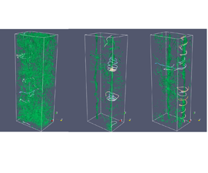
  $\perp$ indicate the wavevectors parallel and perpendicular to the axis of rotation, respectively. Mininni & Pouquet (Reference Mininni and Pouquet2010b) discussed flow structures in detail. They found that strongly helical structures exist in both laminar and time-varying vortex tangles and that the former tangles live for a much longer time. In helical rotating turbulence, anisotropy at small scales is also of interest to researchers. Mininni et al. (Reference Mininni, Rosenberg and Pouquet2012) presented a detectable trend of small-scale isotropy using a DNS of
  $3072^{3}$ points, where the isotropy was recovered at
  $k_\varOmega$. Vallefuoco, Naso & Godeferd (Reference Vallefuoco, Naso and Godeferd2018) performed numerous simulations and found that as wavenumbers increase, the anisotropy decreases at first and then remains unchanged until the minimum scale. Considering the balance between the dissipative and rotating time scales, Vallefuoco et al. (Reference Vallefuoco, Naso and Godeferd2018) also proposed a new scale where the anisotropy becomes unchanged.
As discussed above, the helical rotating turbulence is still not fully understood. In this paper, we mainly address the energy and helicity transfers in helical rotating turbulence. The paper is organized as follows. In § 2, we give the derivation and properties of the energy and helicity transfers. The details of simulations and global behaviours are described in § 3. Next, in § 4, we analyse the transfers of energy and helicity from the perspectives of chirality and anisotropy. The flow structures are shown and illustrated in § 5. Finally, conclusions are given in § 6.
2. Transfers of energy and helicity
The incompressible N–S equations are
 \begin{equation} \left.\begin{gathered} \frac{\partial {\boldsymbol u}}{\partial t} +({\boldsymbol u} \boldsymbol{\cdot} {\boldsymbol\nabla}){\boldsymbol u}={-}{\boldsymbol\nabla} p +\nu \nabla^{2} {\boldsymbol u}+{\boldsymbol f} +2 {\boldsymbol u }\times {\boldsymbol \varOmega}, \\ \boldsymbol{\nabla}\boldsymbol{\cdot} \boldsymbol{u} =0, \end{gathered}\right\} \end{equation}
where  $\boldsymbol {u}$ is the velocity,
  $p$ is the total pressure including the centrifugal effects (Davidson Reference Davidson2010),
  $\nu$ is the kinematic viscosity,
  $\boldsymbol {f}$ is the forcing term and
  $\boldsymbol {\varOmega }$ is the rotating vector and is aligned with the
  $x_3$ axis.
2.1. Energy transfers
The energy transfer equation in spectral space can be deduced from (2.1) as
 \begin{equation} \frac{\partial E(\boldsymbol{k} )}{\partial t}+2\nu \left|\boldsymbol{k}\right| ^{2} E(\boldsymbol{k} )= \sum_{\boldsymbol{p}, \boldsymbol{q} }^{\varDelta} T_E(\boldsymbol{k} |\boldsymbol{p} |\boldsymbol{q} ) + {{\rm Re}} \{\hat{\boldsymbol{u} }^{{\ast}}(\boldsymbol{k}) \boldsymbol{\cdot} \hat{\boldsymbol{f}} (\boldsymbol{k} )\}, \end{equation}
where  $E(\boldsymbol {k} )=\hat {\boldsymbol {u}} (\boldsymbol {k} )\boldsymbol {\cdot } \hat {\boldsymbol {u}}^{\ast }(\boldsymbol {k} )/2$ is the energy at wavenumber
  $\boldsymbol {k}$,
  $\widehat {\;}$ represents the quantity in spectral space, the superscript
  $\ast$ represents the conjugate of a complex value,
  ${\textrm {Re}}\{\,{\boldsymbol{\cdot}}\,\}$ is the real part of a complex value and the symbol
  $\sum _{\boldsymbol {p}, \boldsymbol {q}}^{\varDelta }$ represents a sum over all values of
  $\boldsymbol {p}$ and
  $\boldsymbol {q}$ with
  $\boldsymbol {p} +\boldsymbol {q} +\boldsymbol {k}=\boldsymbol {0}$.
The nonlinear energy transfer  $T_E(\boldsymbol {k} |\boldsymbol {p} |\boldsymbol {q})$ in (2.2) is written as
 \begin{equation} T_E(\boldsymbol{k} |\boldsymbol{p} |\boldsymbol{q} )= {{\rm Re}} \{ \hat{\boldsymbol{u}} (\boldsymbol{k} )\boldsymbol{\cdot} [\hat{\boldsymbol{u}} (\boldsymbol{p} ) \times \hat{\boldsymbol{\omega} } (\boldsymbol{q} ) ]\}, \end{equation}
where  $\hat {\boldsymbol {\omega }}(\boldsymbol {q})=\textrm {i}\boldsymbol {q}\times \hat {\boldsymbol {u}} (\boldsymbol q)$ is the vorticity in spectral space at the wavenumber
  $\boldsymbol {q}$. Utilizing the incompressible constraint
  $\boldsymbol {q}\boldsymbol {\cdot } \hat {\boldsymbol {u}} (\boldsymbol q)=0$, the following property holds:
 \begin{equation} T_E(\boldsymbol{k}|\boldsymbol{p}|\boldsymbol{q})={-}T_E(\boldsymbol{p}|\boldsymbol{k}|\boldsymbol{q}). \end{equation}
This property is named ‘antisymmetry’ for briefness hereafter (Mininni, Alexakis & Pouquet Reference Mininni, Alexakis and Pouquet2006; Mininni et al. Reference Mininni, Alexakis and Pouquet2009), and is the basis of the following analyses. The antisymmetry of  $T_E(\boldsymbol {k}|\boldsymbol {p}|\boldsymbol {q})$ implies that the energy
  $\boldsymbol {k}$ receives is equal to the energy
  $\boldsymbol {p}$ loses. Here
  $\boldsymbol {q}$ plays the role of mediation only and does not gain or lose any energy. Therefore,
  $T_E(\boldsymbol {k}|\boldsymbol {p}|\boldsymbol {q})$ transfers energy from
  $\boldsymbol {p}$ to
  $\boldsymbol {k}$ through
  $\boldsymbol {q}$.
The definition of the nonlinear energy transfer in (2.3) is based on a single triad interaction. To study the properties of the transfer process, the sum of triad interactions needs to be considered. The energy flux is defined as
 \begin{equation} \varPi_E(k=k_1) ={-}\sum_{|\boldsymbol{k}|\le k_1} \sum_{\boldsymbol{p},\boldsymbol{q}}^{\varDelta}T_E(\boldsymbol{k}|\boldsymbol{p}|\boldsymbol{q}). \end{equation}
Notably,  $\varPi _E(k)$ is conservative, i.e.
 \begin{equation} \varPi_E(k=k_{max})=0, \end{equation}
which can be deduced from the antisymmetry. In fact, when a transfer is antisymmetric, the corresponding flux must be conservative.
In helical flows, since the reflection symmetry is broken, chiralities matter greatly. Helical wave decomposition (HWD), which has been employed in helical non-rotating turbulence (Chen et al. Reference Chen, Chen and Eyink2003), is also applied here. The details of HWD are summarized in Appendix A. By HWD, the energy transfer  $T_E(\boldsymbol {k} |\boldsymbol {p} |\boldsymbol {q} )$ can be divided into eight components as
 \begin{align} T_E(\boldsymbol{k} |\boldsymbol{p} |\boldsymbol{q} ) & =\sum_{s_1={\pm}}\sum_{s_2={\pm}}\sum_{s_3={\pm}}T_E^{s_1,s_2, s_3} (\boldsymbol{k} |\boldsymbol{p} |\boldsymbol{q}) \nonumber\\ & =\sum_{s_1={\pm}}\sum_{s_2={\pm}}\sum_{s_3={\pm}}{{\rm Re}} \{ \hat{\boldsymbol{u}}^{s_1} (\boldsymbol{k} )\boldsymbol{\cdot} [ \hat{\boldsymbol{u}}^{s_2} (\boldsymbol{p} ) \times \hat{\boldsymbol{\omega} }^{s_3} (\boldsymbol{q} ) ]\}, \end{align}
where  $s_1,s_2$ and
  $s_3$ represent the charities.
Similar to (2.5), the decomposed energy flux  $\varPi _E^{s_1,s_2,s_3} (k)$ can be defined by
  $T_E^{s_1,s_2,s_3} (\boldsymbol {k}|\boldsymbol {p}|\boldsymbol {q})$. When
  $s_1=s_2=s$,
  $T_E^{s,s,s_3} (\boldsymbol {k} |\boldsymbol {p} |\boldsymbol {q} )$ is antisymmetric, which is the energy transfer in a single chirality. Thus, the corresponding flux
  $\varPi _E^{s,s,s_3} (k)$ is conservative, which is called the conservative flux (Alexakis Reference Alexakis2017). In contrast, when
  $s_1=- s_2=s$,
  $T_E^{s,-s,s_3} (\boldsymbol {k} |\boldsymbol {p} |\boldsymbol {q} )$ is the energy transfer between the two chiralities, which is called the transhelical energy transfer (Alexakis Reference Alexakis2017). This type of energy transfer is not antisymmetric. However, there is another relation describing the transhelical energy transfer:
 \begin{equation} T_E^{s,-s,s_3} (\boldsymbol{k} |\boldsymbol{p} |\boldsymbol{q} )={-}T_E^{{-}s,s,s_3} (\boldsymbol{p} |\boldsymbol{k} |\boldsymbol{q} ). \end{equation}
Therefore, adding in pairs can lead to an antisymmetric transfer, i.e.
 \begin{equation} T_E^{s_3,th} (\boldsymbol{k} |\boldsymbol{p} |\boldsymbol{q} )= T_E^{s,-s,s_3} (\boldsymbol{k} |\boldsymbol{p} |\boldsymbol{q} )+T_E^{{-}s,s,s_3} (\boldsymbol{k} |\boldsymbol{p} |\boldsymbol{q} ). \end{equation}
The related flux  $\varPi _E^{s_3,th} (k)$ is defined by
  $T_E^{s_3,th} (\boldsymbol {k} |\boldsymbol {p} |\boldsymbol {q} )$ in the same way as (2.5). It is conservative and is called the averaged transhelical energy flux.
To illustrate the transfer direction of different fluxes, the spectral space can be divided into two components by a certain wavenumber  $k_1$:
 \begin{equation} R_1(k_1)=\{0\le k\le k_1 \},\quad R_2(k_1)=\{k_1< k\le k_{max}\}, \end{equation}
which is shown in figure 1. Considering chiralities,  $R_i\ (i=1,2)$ can be further partitioned into
  $R_i^{s}$, where the superscript
  $s$ represents the chirality. By the division above,
  $\varPi _E^{s_1,s_2,s_3} (k=k_1)$ can be interpreted as follows.
(i) The conservative energy flux:
 $s_1=s_2=s$, the flux of energy from $R_1^{s}$ to $R_2^{s}$ by the field with the chirality $s_3$.
(ii) The transhelical energy flux:
$s_1=-s_2=s$, the flux of energy from $R_1^{s}$ to $R_1^{-s}$ and $R_2^{-s}$ by the field with the chirality $s_3$.


Figure 1. Division of the spectral space. The spectral space can be divided into five sectors. It can also be divided into  $R_1$ and
  $R_2$ by
  $k_1$ or be divided into
  $S_1$ and
  $S_2$ by
  $\theta _1$. Here,
  $k_1$ and
  $\theta _1$ are certain values of
  $k$ and
  $\theta$, where
  $\theta =\arccos {|k_\parallel |/k}$.
The above explanations are deduced from the antisymmetry of  $T_E^{s_1,s_2,s_3}$ (2.8).
2.2. Helicity transfers
From (2.1), the helicity spectral transfer equation can be derived as
 \begin{equation} \frac{\partial H(\boldsymbol{k})}{\partial t}+2\nu |\boldsymbol{k}|^{2} H(\boldsymbol{k})= \sum_{\boldsymbol{p}, \boldsymbol{q} }^{\varDelta} T_{H}(\boldsymbol{k} |\boldsymbol{p} |\boldsymbol{q} ) +{{\rm Re}}\{\hat{\boldsymbol{\omega}}^{{\ast}}(\boldsymbol{k}) \boldsymbol{\cdot} \hat{\boldsymbol{f}}(\boldsymbol{k})\}, \end{equation}
where  $H(\boldsymbol {k})= {\textrm {Re}}\{\hat {\boldsymbol {u}} (\boldsymbol {k})\boldsymbol {\cdot }\hat {\boldsymbol {\omega }}^{\ast }(\boldsymbol {k})\} /2$ is the helicity at the wavenumber
  $\boldsymbol {k}$ (Polifke & Shtilman Reference Polifke and Shtilman1989),
  $T_{H}(\boldsymbol {k} |\boldsymbol {p} |\boldsymbol {q} )$ is the first expression of the nonlinear helicity transfer. See Appendix B.1 for the details of the derivations.
2.2.1. Three expressions of the helicity transfer
There are three expressions for the helicity transfer of a single triad,
 \begin{gather} T_{H} (\boldsymbol{k} |\boldsymbol{p} |\boldsymbol{q} ) = \tfrac{1}{2}{{\rm Im}}\{[\boldsymbol{k} \boldsymbol{\cdot} \hat{\boldsymbol{\omega}} (\boldsymbol{q} )][ \hat{\boldsymbol{u}} (\boldsymbol{k} )\boldsymbol{\cdot} \hat{\boldsymbol{u}} (\boldsymbol{p} )]\}-\tfrac{1}{2}{{\rm Im}}\{[\boldsymbol{k} \boldsymbol{\cdot} \hat{\boldsymbol{u}} (\boldsymbol{q} )][ \hat{\boldsymbol{u}} (\boldsymbol{k} )\boldsymbol{\cdot} \hat{\boldsymbol{\omega} } (\boldsymbol{p} )]\} \nonumber\\ \hspace{-4.8pc} -\tfrac{1}{2}{{\rm Im}}\{[\boldsymbol{k} \boldsymbol{\cdot} \hat{\boldsymbol{u}} (\boldsymbol{q} )] [\hat{\boldsymbol{\omega} } (\boldsymbol{k} )\boldsymbol{\cdot} \hat{\boldsymbol{u}} (\boldsymbol{p} )]\}, \end{gather}
 $$\begin{gather} T_{H}'(\boldsymbol{k} |\boldsymbol{p} |\boldsymbol{q} ) ={-}{{\rm Im}}\{[\boldsymbol{k} \boldsymbol{\cdot} \hat{\boldsymbol{u}} (\boldsymbol{q})][\hat{\boldsymbol{\omega} } (\boldsymbol{k}) \boldsymbol{\cdot}\hat{\boldsymbol{u}} (\boldsymbol{p})]\}, \end{gather}$$
 $$\begin{gather}T_{H}''(\boldsymbol{k} |\boldsymbol{p} |\boldsymbol{q} ) = {{\rm Re}}\{\hat{\boldsymbol{\omega}} (\boldsymbol{k})\boldsymbol{\cdot} [\hat{\boldsymbol{u}} (\boldsymbol{q}) \times \hat{\boldsymbol{\omega}} (\boldsymbol p)] \}, \end{gather}$$
where  ${\textrm {Im}}\{{\boldsymbol{\cdot} }\}$ denotes the imaginary part of a complex value. The first expression
  $T_{H} (\boldsymbol {k} |\boldsymbol {p} |\boldsymbol {q} )$ can be decomposed into three components (
 $T_{H1} (\boldsymbol {k} |\boldsymbol {p} |\boldsymbol {q}$),
  $T_{H2} (\boldsymbol {k} |\boldsymbol {p} |\boldsymbol {q} )$ and
  $T_{H3} (\boldsymbol {k} |\boldsymbol {p} |\boldsymbol {q} )$, respectively). Here,
  $T_{H1} (\boldsymbol {k}|\boldsymbol {p}|\boldsymbol {q})$ and
  $T_{H2} (\boldsymbol {k}|\boldsymbol {p}|\boldsymbol {q})$ are associated with the vortex stretching process, and
  $T_{H3} (\boldsymbol {k}|\boldsymbol {p}|\boldsymbol {q})$ is related to the vortex twisting process (Eyink Reference Eyink2006; Yan et al. Reference Yan, Li and Yu2020a,Reference Yan, Li, Yu, Wang and Chenb). The first expression,
  $T_{H} (\boldsymbol {k} |\boldsymbol {p} |\boldsymbol {q} )$, is derived by a similar approach in physical space (Yan et al. Reference Yan, Li, Yu, Wang and Chen2020b). In this paper, it is first discussed in the spectral analyses of helical flows, and its detailed derivations are given in Appendix B.1. The second expression,
  $T_{H}'(\boldsymbol {k} |\boldsymbol {p} |\boldsymbol {q} )$, comes from the advection
  $\boldsymbol {u}\boldsymbol {\cdot }\boldsymbol {\nabla } \boldsymbol {u}$, which has been applied by Chen et al. (Reference Chen, Chen and Eyink2003). The third expression,
  $T_{H}''(\boldsymbol {k} |\boldsymbol {p} |\boldsymbol {q} )$, is derived from the Lamb vector
  $\boldsymbol {u}\times \boldsymbol {\omega }$ (Mininni et al. Reference Mininni, Alexakis and Pouquet2006; Alexakis Reference Alexakis2017).
The three expressions are not equal when only one triad is considered. However, as proved in Appendix B.2.1, the three expressions are identical for the sum of all  $\boldsymbol {p}$ and
  $\boldsymbol {q}$ with
  $\boldsymbol {k}+\boldsymbol {p}+\boldsymbol {q}=0$, i.e.
 \begin{equation} \sum_{\boldsymbol{p},\boldsymbol{q}}^{\varDelta}T_{H} (\boldsymbol{k} |\boldsymbol{p} |\boldsymbol{q} ) = \sum_{\boldsymbol{p},\boldsymbol{q}}^{\varDelta}T_{H}'(\boldsymbol{k} |\boldsymbol{p} |\boldsymbol{q} ) = \sum_{\boldsymbol{p},\boldsymbol{q}}^{\varDelta}T_{H}''(\boldsymbol{k} |\boldsymbol{p} |\boldsymbol{q} ). \end{equation}
As is well known, there is only one expression of helicity transfer in physical space (Yan et al. Reference Yan, Li, Yu, Wang and Chen2020b), which is related to (2.12a) here. The reason for the different three expressions here is the commutability of differential operators in spectral space. Taking part of the derivations in Appendix B.2.1 as examples, the following relations hold:
 $$\begin{gather} {{\rm Re}}\{ \hat{\boldsymbol{u}}^{{\ast}}\boldsymbol{\cdot} \mathcal{F}\{\boldsymbol{\nabla}\times (\boldsymbol{u} \times \boldsymbol{\omega})\}\} = {{\rm Re}}\{\hat{\boldsymbol{\omega}}^{{\ast}} \boldsymbol{\cdot} \mathcal{F}\{{\boldsymbol{u}} \times {\boldsymbol{\omega}} \} \}, \end{gather}$$
 $$\begin{gather}{\boldsymbol{u}}\boldsymbol{\cdot} [\boldsymbol{\nabla}\times (\boldsymbol{u} \times \boldsymbol{\omega})] ={\boldsymbol{\omega}} \boldsymbol{\cdot} (\boldsymbol{u} \times \boldsymbol{\omega}) +\boldsymbol{\nabla}\boldsymbol{\cdot} [(\boldsymbol{u} \times \boldsymbol{\omega})\times {\boldsymbol{u}}], \end{gather}$$
where  $\mathcal {F}\{{\cdot }\}$ represents the Fourier transform. Equation (2.14a) is in spectral space, and (2.14b) is in physical space. As shown by these relations, the differential operators commute with other terms in spectral space, while commuting in physical space could introduce another gradient.
Moreover, in §§ 2.2.2, 4.2 and Appendix B.2, more relations about helicity transfers and fluxes are discussed. It is demonstrated that the three expressions are truly different. Only the expression derived here (2.12a) is directly associated with the expression in physical space.
2.2.2. Properties of helicity transfers and fluxes
It can be deduced from the definition of the helicity transfer that  $T_{H} (\boldsymbol {k} |\boldsymbol {p} |\boldsymbol {q} )$ and
  $T_{H}''(\boldsymbol {k} |\boldsymbol {p} |\boldsymbol {q} )$ satisfy antisymmetry, while
  $T_{H}'(\boldsymbol {k} |\boldsymbol {p} |\boldsymbol {q} )$ does not. Therefore,
  $T_{H} (\boldsymbol {k} |\boldsymbol {p} |\boldsymbol {q} )$ and
  $T_{H}''(\boldsymbol {k} |\boldsymbol {p} |\boldsymbol {q} )$ have clear physical meanings. The first expression of the helicity flux is written as
 \begin{equation} \varPi_H(k=k_1) ={-}\sum_{|\boldsymbol{k}|\le k_1} \sum_{\boldsymbol{p},\boldsymbol{q}}^{\varDelta}T_H(\boldsymbol{k}|\boldsymbol{p}|\boldsymbol{q}). \end{equation}
Similar to (2.15),  $\varPi _{Hi} (k)\ (i=1,2,3)$,
  $\varPi _H'(k)$ and
  $\varPi _H''(k)$ can be defined by
  $T_{Hi} (\boldsymbol {k}|\boldsymbol {p}|\boldsymbol {q})\ (i=1,2,3)$,
  $T_H'(\boldsymbol {k}|\boldsymbol {p}|\boldsymbol {q})$ and
  $T_H''(\boldsymbol {k}|\boldsymbol {p}|\boldsymbol {q})$, respectively. According to (2.13), the three fluxes are equal, i.e.
 \begin{equation} \varPi_H(k)=\varPi_H'(k)=\varPi_H''(k), \end{equation}
where  $\varPi _H(k)$ includes three components
  $\varPi _{Hi} (k) (i=1,2,3)$.
For the results of HWD,  $T_H''(\boldsymbol {k} |\boldsymbol {p} |\boldsymbol {q} )$ can be decomposed as
 \begin{align} T_H''(\boldsymbol{k} |\boldsymbol{p} |\boldsymbol{q}) &= \sum_{s_1={\pm}}\sum_{s_2={\pm}}\sum_{s_3={\pm}}T_H''^{\,s_1,s_2, s_3} (\boldsymbol{k} |\boldsymbol{p} |\boldsymbol{q}) \nonumber\\ &= \sum_{s_1={\pm}}\sum_{s_2={\pm}}\sum_{s_3={\pm}}{{\rm Re}}\{\hat{\boldsymbol{\omega}}^{s_1} (\boldsymbol{k})\boldsymbol{\cdot} \hat{\boldsymbol{u}}^{s_2} (\boldsymbol{q}) \times \hat{\boldsymbol{\omega}}^{s_3} (\boldsymbol p) \}, \end{align}
where the superscripts  $s_1, s_2$ and
  $s_3$ correspond to the field at wavenumbers
  $\boldsymbol {k}$,
  $\boldsymbol {q}$ and
  $\boldsymbol {p}$, respectively (Alexakis Reference Alexakis2017). Here
  $T_H^{s_1,s_2, s_3} (\boldsymbol {k} |\boldsymbol {p} |\boldsymbol {q} )$ can be defined in the same way.
Similar to (2.15), the decomposed helicity fluxes ( $\varPi _H^{s_1,s_2,s_3} (k$) and
  $\varPi _H''^{\,s_1,s_2,s_3} (k)$) are defined by
  $T_H^{s_1,s_2,s_3} (\boldsymbol {k}|\boldsymbol {p}|\boldsymbol {q})$ and
  $T_H''^{\,s_1,s_2,s_3} (\boldsymbol {k}|\boldsymbol {p}|\boldsymbol {q})$, respectively. By the division shown in figure 1,
  $\varPi _H^{s_1,s_2,s_3}\ (k=k_1)$ can be interpreted as follows.
(i) The conservative helicity flux:
$s_1=s_3=s$, the flux of helicity from $R_1^{s}$ to $R_2^{s}$ by the field with the chirality $s_2$.(ii) The transhelical helicity flux:
$s_1=-s_3=s$, the flux of helicity from $R_1^{s}$ to $R_1^{-s}$ and $R_2^{-s}$ by the field with the chirality $s_2$.


It has been proved in Appendix B.2.3 that only when  $s_2=s_3=s$ will the first and the third expressions of the decomposed helicity fluxes be equal, viz.
 \begin{equation} \varPi_H^{s_1,s,s} (k)=\varPi_H''^{\,s_1,s,s} (k). \end{equation}
 Since  $T_H^{s_1,s_2, s_3} (\boldsymbol {k} |\boldsymbol {p} |\boldsymbol {q} )$ and
  $T_H''^{\,s_1,s_2, s_3} (\boldsymbol {k} |\boldsymbol {p} |\boldsymbol {q} )$ are the same when considering antisymmetry and conservation, only the properties of
  $T_H^{s_1,s_2, s_3} (\boldsymbol {k} |\boldsymbol {p} |\boldsymbol {q} )$ are discussed here. When
  $s_1=s_3=s$,
  $T_H^{s,s_2,s} (\boldsymbol {k} |\boldsymbol {p} |\boldsymbol {q} )$ satisfies antisymmetry, which can be interpreted as the helicity transfer in a single chirality. The corresponding flux is called the conservative helicity flux (Alexakis Reference Alexakis2017). Otherwise,
  $T_H^{s,s_2,-s} (\boldsymbol {k} |\boldsymbol {p} |\boldsymbol {q} )$ is the transfer between the two chiralities and is not antisymmetric. The corresponding flux
  $\varPi _H^{s,s_2,-s} (k)$ is called the transhelical helicity flux (Alexakis Reference Alexakis2017). Here
  $T_H^{s_2,th} (\boldsymbol {k} |\boldsymbol {p} |\boldsymbol {q} )$ can be obtained by adding
  $T_H^{s,s_2,-s} (\boldsymbol {k} |\boldsymbol {p} |\boldsymbol {q} )$ in pairs,
 \begin{equation} T_H^{s_2,th} (\boldsymbol{k} |\boldsymbol{p} |\boldsymbol{q} )= T_H^{s,s_2,s} (\boldsymbol{k} |\boldsymbol{p} |\boldsymbol{q} )+T_H^{{-}s,s_2,s} (\boldsymbol{k} |\boldsymbol{p} |\boldsymbol{q} ), \end{equation}
which is antisymmetric. The relative flux  $\varPi _H^{s_2,th} (k)$ is conservative and is called the averaged transhelical helicity flux. Similar to energy, for the transhelical transfers of helicity, there is another relation:
 \begin{equation} T_H^{s,s_2,-s} (\boldsymbol{k} |\boldsymbol{p} |\boldsymbol{q} )={-}T_H^{{-}s,s_2,s} (\boldsymbol{p} |\boldsymbol{k} |\boldsymbol{q} ). \end{equation}
In addition,  $T_H''^{\,s_2,th} (\boldsymbol {k} |\boldsymbol {p} |\boldsymbol {q} )$ and
  $\varPi _H''^{\,s_2,th} (k )$ are defined by
  $T_H''^{\,s_1,s_2,s_3} (\boldsymbol {k} |\boldsymbol {p} |\boldsymbol {q} )$ similar to (2.19) and (2.15), respectively.
In summary, the antisymmetry of transfers is the sufficient condition for the conservation of related fluxes, regardless of energy or helicity. The conservative flux represents the flux in a single chirality, while the (averaged) transhelical flux represents the flux between the two chiralities. The conservative and averaged transhelical fluxes are conservative. In contrast, the transhelical flux is not conservative. Additionally, when  $s_1=s_2=s_3=s$,
  $\varPi _E^{s,s,s} (k)$ and
  $\varPi _H^{s,s,s} (k)$ are homochiral fluxes. Otherwise,
  $\varPi _E^{s_1,s_2,s_3} (k)$ and
  $\varPi _H^{s_1,s_2,s_3} (k)$ are heterochiral fluxes.
3. Numerical simulations
3.1. Numerical set-up
Seven DNSs with  $1536^{3}$ grid points are carried out. A 2-D parallel pseudospectral code is implemented to solve the incompressible N–S equations (2.1). In addition, the explicit second-order Adams–Bashforth technique is performed for temporal evolution.
There are two forcing schemes. Since different relative helicity injection rates are needed to study the influence of helicity, the forcing scheme of Teimurazov et al. (Reference Teimurazov, Stepanov, Verma, Barman, Kumar and Sadhukhan2018) is applied,
 \begin{equation} \hat{\boldsymbol{f}} (\boldsymbol{k} )=A \hat{\boldsymbol{u}} (\boldsymbol{k} ) +B \hat{\boldsymbol{\omega}} (\boldsymbol{k} ), \end{equation}
which is named Tei18 hereafter. Given the energy injection  $\epsilon _E$ and the helicity injection
  $\epsilon _H$, the parameters
  $A$ and
  $B$ are determined as
 \begin{equation} A=\frac{1}{2}\frac{W_f\epsilon_E-H_f \epsilon_H}{E_f W_f -H_f^{2}},\quad B=\frac{1}{2}\frac{E_f\epsilon_H-H_f\epsilon_E}{E_fW_f-H_f^{2}}, \end{equation}
where  $E_f=\sum _{|\boldsymbol {k}|\in k_f}\frac {1}{2}|\hat {\boldsymbol {u}} (\boldsymbol {k})|^{2}$,
  $H_f=\sum _{|\boldsymbol {k}|\in k_f}\frac {1}{2}{\textrm {Re}}\{\hat {\boldsymbol {u}}(\boldsymbol {k}) \boldsymbol {\cdot }\hat {\boldsymbol {\omega } }^{\ast } (\boldsymbol {k})\}$ and
  $W_f=\sum _{|\boldsymbol {k}|\in k_f} \frac {1}{2}k^{2}|\hat {\boldsymbol {u}} (\boldsymbol {k})|^{2}$ are energy, helicity and enstrophy at the forcing scale
  $k_f$, respectively. In addition, to exclude the artificial effects of the forcing scheme, the Arnold–Beltrami– Childress (ABC) forcing scheme (Mininni & Pouquet Reference Mininni and Pouquet2009) is also considered, which can be written in physical space as
 \begin{align} \boldsymbol{f} (\boldsymbol{x}) &= F_0\{[B\cos(k_f x_2)+C\sin(k_f x_3)] \boldsymbol{e}_1 +[C\cos(k_f x_3)+A\sin(k_f x_1)] \boldsymbol{e}_2 \nonumber\\ &\quad +[A\cos(k_f x_1)+B\sin(k_f x_2)] \boldsymbol{e}_3\}, \end{align}
where  $A=0.9$,
  $B=1.0$,
  $C=1.1$;
  $\boldsymbol {e}_i$ is the unit vector of corresponding axis; and
  $F_0$ is determined by the given energy injection rate
  $\epsilon _E$. The ABC forcing scheme can only inject maximum helicity, i.e.
  $\epsilon _H=k_f\epsilon _E$. Notably, in both forcing schemes above, the forcing term is a solenoid vector, i.e.
  $\textrm {i}\boldsymbol {k} \boldsymbol {\cdot }\hat {\boldsymbol {f}} (\boldsymbol {k})=0$.
In helical rotating turbulence, the Reynolds and Rossby numbers are defined as
 \begin{equation} Re=\frac{L_fU}{\nu},\quad Ro=\frac{U}{2\varOmega L_f}, \end{equation}
where  $Re$ represents the ratio of the inertial force and the viscous force,
  $Ro$ is the ratio of the inertial force and the Coriolis force,
  $L_f=2{\rm \pi} /k_f$ is the forcing scale and
  $U=\sqrt {\langle u^{2} \rangle }$ is the root mean square velocity. The main arguments are listed in table 1, where the eddy turnover time is
  $T_0=L_f/U$. Since TD3 starts from T3 and freely decays,
  $Re,Ro$ and
  $T_0$ of TD3 are the same as T3, its relative helicity is calculated at 2.5 eddy turnover times. Other common parameters include the forcing wavenumbers
  $k_f= 7$ and the kinematic viscosity
  $\nu =2\times 10^{-4}$.
Table 1. Descriptions of the data: rotation rate ( $\varOmega$); energy injection rate (
 $\epsilon _E$); helicity injection rate (
 $\epsilon _H$); relative helicity injection rate (
 $\epsilon _H/k_f\epsilon _E$); relative helicity at
  $k_f$ (
 $H_f/k_fE_f$); Reynolds number (
 $Re$); Rossby number (
 $Ro$); the forcing scheme (forcing); eddy turnover time (
 $T_0$).

The simulations first reach a balance with  $\varOmega =0.06$ and
  $768^{3}$ grid points. Then, T0 is interpolated to
  $1536^{3}$ grid points and continues for 6.61 eddy turnover times with
  $\varOmega =0$, which is steady after the first 1.4 eddy turnover times. Other cases except for TD3 continue for approximately nine eddy turnover times with
  $768^{3}$ grid points and
  $\varOmega$ in table 1. Finally, these cases are interpolated to
  $1536^{3}$ grid points and continue for approximately five eddy turnover times. The exact moments of interpolation are marked by triangles in figure 2, when the trend of evolution is monotonic. Starting from T3 at 11.6 eddy turnover times, TD3 continues for 4.9 eddy turnover times with no injection.

Figure 2. Temporal evolution of the averaged (a) energy and (b) helicity. The triangles represent the time when interpolation is performed. The blocks represent the time when numerical results are calculated.
Here, T0 has a zero rotation rate but maximum helicity injection; T1, T2 and T3 have the same rotation rate but different helicity injection rates; T4 has a smaller rotation rate than T3; TD3 has no energy or helicity injection. Except for the forcing scheme, ABC3 has the same arguments as T3.
3.2. Global behaviours
Figure 2 presents the evolution of the averaged energy  $E=\langle \boldsymbol {u} (\boldsymbol {x})\boldsymbol {\cdot }\boldsymbol {u} (\boldsymbol {x}) \rangle /2$ and helicity
  $H=\langle \boldsymbol {u} (\boldsymbol {x})\boldsymbol {\cdot }\boldsymbol {\omega } (\boldsymbol {x}) \rangle /2$. The time in the figure is normalized by the eddy turnover time. In figure 2(a), after a transition of no more than six eddy turnover times,
  $E$ of T1 and T2 develops faster than that of T3 and ABC3, which means that strong helicity can inhibit the rate of energy increase. In figure 2(b),
  $H$ of T1 varies around zero, which involves no helicity injection. Additionally,
  $H$ of T2 and T4 is approximately steady. In T3 and ABC3, where nearly maximum helicity is injected, the helicity initially increases and then decreases. The energy and helicity of TD3 decrease monotonically. If not specified, the numerical results hereafter are calculated at the time marked by blocks in figure 2.
The isotropic spectra of energy and helicity are defined as
 \begin{equation} E(k)=\sum_{|\boldsymbol{k}|=k}E(\boldsymbol{k}),\quad H(k)=\sum_{|\boldsymbol{k}|=k}H(\boldsymbol{k}). \end{equation}
Figure 3 shows the energy and helicity spectra of all cases. Without rotation, the scaling laws of the energy and helicity spectra of T0 are shallower than  $k^{-5/3}$. Similar results have been reported by other researchers (Mininni & Pouquet Reference Mininni and Pouquet2010b; Alexakis & Biferale Reference Alexakis and Biferale2018). Moreover, with a relatively small rotation rate (
 $\varOmega =4$), the scaling law of the energy spectrum of T4 presents two different behaviours:
  $E(k)\sim k^{-2.2}$ when
  $k<20$, and
  $E(k)\sim k^{-5/3}$ when
  $k>20$. This can be attributed to the recovery of isotropy at small scales and is consistent with the results of Mininni et al. (Reference Mininni, Rosenberg and Pouquet2012). In addition, except for T0 and T4, the scaling laws of the energy spectra are nearly
  $k^{-2.2}$ for all cases. However, as the helicity injection becomes stronger from T1 to T3, the energy spectra become slightly shallower from
  $k^{-2.2}$ to
  $k^{-2.15}$. Furthermore, ABC3 and T3 have the same slope in the inertial range, which means that the forcing schemes have negligible effects here. For the cases except for T0, T1 and T4, the scaling laws of the helicity spectra are close to
  $k^{-1.8}$. The helicity spectrum of T1 oscillates violently, which can be attributed to the absence of helicity injection. Additionally, the net helicity of T1 is positive at a wide range of wavenumbers, which is just a special case. The helicity spectrum generally oscillates around zero during the whole evolution process.

Figure 3. Compensated spectra of energy and helicity: (a)  $E(k)k^{2.2}$; (b)
  $H(k)k^{1.8}$.
Furthermore, Galtier (Reference Galtier2014) has derived the cospectrum of  $E(k)H(k)\sim k^{-4}$, which has also been addressed by numerical simulations (Mininni & Pouquet Reference Mininni and Pouquet2010a). In our simulation, the scaling laws of the cospectra of TD3, T2, T3 and ABC3 vary from
  $k^{-4.0}$ to
  $k^{-3.9}$. Figure 4 gives the evolution of the compensated spectra
  $E(k)H(k)k^{4}$ of T2 and T3. The spectra mainly vary at the early six eddy turnover times. In the later stage, the small-scale spectra (
 $k\ge 15$) are almost unaffected, while the amplitudes of the large-scale spectra keep growing. In addition, the interpolation has small effects on the evolution of the spectra in the inertial range.

Figure 4. Temporal evolution of compensated spectra: (a) T2; (b) T3.
The decomposed energy spectrum  $E^{s}(k)$ is defined by (A5). Figure 5 shows
  $E^{s}(k)$ of T1 and T3. As shown in figure 5(a), without any helicity injection, the two chiralities of T1 are far from distinguishable. In contrast, in T3, the imbalance of chiralities mainly occurs around the forcing wavenumber
  $k_f$. At small scales (
 $k\gtrapprox 10^{2}$) and the largest scale (
 $k\approx 1$), the reflection symmetry is recovered.

Figure 5. Decomposed energy spectra after HWD: (a) T1; (b) T3.
Considering the anisotropy, a spectrum can be divided into  $N$ sectors according to the angle (
 $\theta \in [0,{\rm \pi} /2]$) between the wavevector and the rotating axis,
 \begin{equation} E(k,\alpha) =\sum_{|\boldsymbol{k}|=k}\sum_{\theta_{\alpha-1}< \theta\le\theta_{\alpha}} E(\boldsymbol{k}), \end{equation}
where  $\theta =\arccos ({k_\parallel }/{k})$,
  $\theta _\alpha ={\rm \pi} \alpha /2N$ is the angle of different sector boundaries and
  $\alpha =\{1, \ldots,N\}$ is the index of sectors. Figure 1 gives the division of the spectral space into five sectors. To study the anisotropy in detail, the relative difference of the directional spectrum and corresponding isotropic spectrum is introduced (Vallefuoco et al. Reference Vallefuoco, Naso and Godeferd2018),
 \begin{equation} {\rm \Delta} E(k,\alpha) = \frac{1}{|\cos(\theta_\alpha)-\cos(\theta_{\alpha-1})|} \frac{E(k,\alpha)}{E(k)}-1, \end{equation}
where  $N=5$ in this paper. Since
  $E(k,\alpha )\ge 0$,
  ${\rm \Delta} _{E} (k,\alpha )\ge -1$.
Figure 6 presents the results of anisotropy of T2, T3, ABC3 and T4. In general, for most wavenumbers, energy is concentrated in sector  $5$, which means the two-dimensionalization of flows. The comparison of figure 6(a) with figure 6(b) indicates that as the helicity injection becomes stronger, the energy at
  $k_f$ tends to concentrate on sector
  $1$. However, the comparison of figure 6(b) with figure 6(c) reveals that the abnormal distribution at
  $k_f$ in figure 6(b) is introduced by the forcing scheme Tei18. The artificial effects are limited to wavenumbers
  $[4,20]$. Similar artificial effects can also be identified in figure 6(d). Nonetheless, figure 6(d) still carries important information about the recovery of small-scale isotropy. As shown in the figure, the non-dimensional directional spectra at small scales do not recover to fully isotropic, and they do not reach constant values until
  $k>60$, which is consistent with the results of Vallefuoco et al. (Reference Vallefuoco, Naso and Godeferd2018). Furthermore, Mininni et al. (Reference Mininni, Rosenberg and Pouquet2012) argued that small scales recover to isotropy mainly by the transition of energy scaling laws. A similar tendency is also shown in figure 3(a) in this paper. However, the results here reveal that even if the scaling law is similar to the isotropic case, the small scales are still not fully isotropic. At small scales (
 $k>70$) of T4, sector 5 contains approximately 1.5 times as much energy as sector 1.

Figure 6. The results of anisotropy: (a) T2; (b) T3; (c) ABC3; (d) T4.
4. Results of transfers
The scale transfer is complicated, especially considering the chirality and anisotropy in helical rotating turbulence. However, transfer analyses are significant for understanding and modelling the process (Chen et al. Reference Chen, Chen and Eyink2003). In helical rotating turbulence, attributed to its complexity, detailed analyses of the transfer processes are still scarce.
4.1. Energy transfers
According to the antisymmetry of  $T_E(\boldsymbol {k}|\boldsymbol {p}|\boldsymbol {q})$ (2.4),
  $\varPi _E(k=k_1)$ represents the energy flux from
  $[0, k_1]$ to
  $(k_1,k_{max}]$. In figure 7, the energy fluxes of all cases are given. In this paper, all fluxes are normalized by corresponding injection rates except for TD3. The fluxes of TD3 hereafter are normalized by the parameters of T3.

Figure 7. Overall energy fluxes. The black horizontal line represents zero flux for reference.
With a zero rotation rate, T0 cascades energy forward only. Other cases cascade energy upscale and downscale simultaneously. As more helicity is injected (from T1 to T3), the inverse cascades become weaker. As the rotation rate decreases from T3 to T4, the inverse cascades are also significantly suppressed. The suppression of inverse cascades can be associated with the smaller rate of energy increase shown in figure 2(a). This is because energy is mainly contained at large scales where dissipation is negligible. The rate of energy increase is approximately proportional to the strength of inverse cascades.
4.1.1. Energy fluxes decomposed by HWD
Figure 8 gives the results of decomposed energy fluxes of T0, T1, T3 and ABC3. The results in figure 8(a) are consistent with those of Alexakis (Reference Alexakis2017). With the zero rotation rate in T0, the inverse energy cascade is hidden in the overall forward cascade and is supported by the homochiral fluxes ( $\varPi _E^{+++} (k)+\varPi _E^{---} (k$)). The comparison of figure 8(a) with figure 8(c) indicates that as rotation is introduced, the inverse cascade of the homochiral fluxes is strengthened. Additionally, inverse cascades are also introduced by conservative heterochiral fluxes (
 $\varPi _E^{++-} (k)+\varPi _E^{--+} (k$)) and averaged transhelical energy fluxes (
 $\varPi _E^{+,th} (k)+\varPi _E^{-,th} (k$)), where the former fluxes have a minor effect. Notably, the two classes of fluxes are heterochiral. Similar results were reported by Buzzicotti et al. (Reference Buzzicotti, Aluie, Biferale and Linkmann2018a), who associated homochiral energy fluxes with the interactions of 3-D modes and heterochiral energy fluxes with the interactions of 2-D modes. To evaluate the effects of helicity injection, figures 8(b) and 8(c) are compared. As helicity is injected, the overall inverse cascades are suppressed. The homochiral fluxes are relatively unaffected, while the inverse cascades of the averaged transhelical energy fluxes are suppressed. This is also supported by the results of ABC3 in figure 8(d) and of T3 at another instant (not shown here). The averaged transhelical energy fluxes are the fluxes between the two chiralities and are associated with the 2-D modes according to the research of Buzzicotti et al. (Reference Buzzicotti, Aluie, Biferale and Linkmann2018a). Therefore, the reduction of the inverse cascades and energy growth rate can be attributed to the injection of helicity suppressing the interactions of two chiralities as well as those of 2-D modes. The suppression of 2-D interactions is in agreement with previous results, since helicity does not work in 2-D dynamics (Biferale, Buzzicotti & Linkmann Reference Biferale, Buzzicotti and Linkmann2017).

Figure 8. Results of energy flux decomposition: (a) T0; (b) T1; (c) T3; (d) ABC3.
Figure 9 shows the detailed energy flux decomposition of T3. The results of ABC3 in Appendix C are consistent with those in figure 9 and are not discussed here. As predicted, all four transhelical energy fluxes are not conservative. In addition, since the injected helicity is positive, the components with more positive modes have larger amplitudes than their symmetric components, such as  $\varPi _E^{+++} (k)$ versus
  $\varPi _E^{---} (k)$ or
  $\varPi _E^{+-+} (k)$ versus
  $\varPi _E^{-+-} (k)$. Furthermore, according to the interpretation given in § 2, since
  $\varPi _E^{+-+} (k)+\varPi _E^{+--} (k)>0$, energy is mainly injected into the positive chirality and then transferred to the negative chirality.

Figure 9. Detailed energy flux decomposition of T3: (a) conservative energy fluxes; (b) transhelical energy fluxes.
The findings of inverse cascades can also be explained in terms of reflection symmetry recovery. Inverse cascades only occur when  $\varPi _E^{s_1,s_2,s_3} (k)<0$, which means that the energy is transferred towards large scales. In helical cases, the positive chirality is dominant. The recovery of the reflection symmetry implies that the dominant chirality loses more energy than another chirality. Thus,
  $\varPi _E^{s_1,+,+} (k)$ (
 $\varPi _E^{+++} (k$) and
  $\varPi _E^{-++} (k)$) dominate the inverse cascades, which is consistent with the numerical results in figure 9.
4.1.2. Anisotropic energy transfers
In helical rotating turbulence, another topic of the energy transfer is the anisotropy. Referring to the definition of the energy anisotropy (3.6), the energy transfer across the angle  $\theta _1$ is written as
 \begin{equation} \varPi_E(\theta=\theta_1)={-}\sum_{p_\parallel{/}|\boldsymbol{p}|\ge\cos\theta_1} \sum_{k_\parallel{/}|\boldsymbol{k}|<\cos\theta_1} \sum_{\boldsymbol{q} ={-}\boldsymbol{p}-\boldsymbol{k}} T_E(\boldsymbol{k}|\boldsymbol{p}|\boldsymbol{q}). \end{equation}
According to the results of figure 6, the forcing scheme Tei18 introduces artificial effects around the forcing wavenumber. Therefore, the small-scale anisotropic energy transfer is also considered here to exclude the effects:
 \begin{equation} \varPi_E^{>}(\theta=\theta_1)={-}\sum_{p_\parallel{/}|\boldsymbol{p}|\ge\cos\theta_1} \sum_{\scriptsize \begin{aligned} & k_\parallel{/}|\boldsymbol{k}|<\cos\theta_1 \\ & |\boldsymbol{k}|> 20 \end{aligned}} \sum_{\boldsymbol{q} ={-}\boldsymbol{p}-\boldsymbol{k}}T_E(\boldsymbol{k}|\boldsymbol{p}|\boldsymbol{q}). \end{equation}
The wavenumbers ( $k>20$) considered in
  $\varPi _E^{>}(\theta )$ include part of the inertial range and the whole dissipative range.
Figure 10 gives the results of  $\varPi _E(\theta )$ and
  $\varPi _E^{>}(\theta )$. As shown in figure 10(a),
  $\varPi _E(\theta )$ of T3 is completely different from that of ABC3, which could be attributed to the artificial effects of the forcing scheme Tei18. Furthermore, considering TD3, even if this case freely decays for 2.5 eddy turnover times, it still maintains the artificial effects of the forcing scheme Tei18. When considering
  $\varPi _E^{>}(\theta )$ at small scales in figure 10(b), various cases lead to similar results. Notably, the results in figure 10(b) show small-scale anisotropy in T4, which is consistent with the anisotropy results in figure 6(d).

Figure 10. Anisotropic energy transfers: (a)  $\varPi _E(\theta )$; (b)
  $\varPi ^{>}_E(\theta )$.
Similar to (4.2), the decomposed anisotropic energy transfers  $\varPi ^{>\,s_1,s_2,s_3}_E(\theta =\theta _1)$ can be defined by
  $T_E^{s_1,s_2,s_3} (\boldsymbol {k}|\boldsymbol {p}|\boldsymbol {q})$. As illustrated in figure 1, the spectral space can be divided into two components by
  $\theta _1$:
 \begin{equation} S_1(k_1)=\{0\le \theta\le \theta_1 \},\quad S_2(k_1)=\{\theta_1<\theta\le {\rm \pi}/2\}. \end{equation}
Furthermore,  $S_i\ (i=1,2)$ can be further partitioned into
  $S_i^{s}$ when chiralities are considered. Here
  $\varPi _E^{s_1,s_2,s_3} (\theta =\theta _1)$ can be interpreted as follows.
(i) The conservative anisotropic energy transfer:
$s_1=s_2=s$, the transfer of energy from $S_1^{s}$ to $S_2^{s}$ by the field with the chirality $s_3$.(ii) The transhelical anisotropic energy transfer:
$s_1=-s_2=s$, the transfer of energy from $S_1^{s}$ to $S_2^{-s}$ by the field with the chirality $s_3$.


Strictly speaking, all components of decomposed anisotropic transfers are conservative, viz.,  $\varPi _E^{s_1,s_2,s_3} (\theta ={\rm \pi} /2)=0$. However, for consistency, we still name those components conservative or transhelical anisotropic energy transfers.
Figure 11 gives  $\varPi ^{>\,s_1,s_2,s_3}_E(\theta )$ of T3, where conservative anisotropic energy transfers are given in figure 11(a) and transhelical anisotropic energy transfers are given in figure 11(b). Notably,
  $\varPi ^{>\,s_1,s_2,s_3}_E(\theta )$ generally has the opposite sign to
  $\varPi ^{s_1,s_2,s_3}_E(k)$. There is only one exception:
  $\varPi ^{>--+}_E(\theta )$ crosses the zero line at
  $\theta =0.4{\rm \pi}$, but it still fits the sign results over the wide range
  $[0,0.4{\rm \pi} ]$. The results of ABC3 in Appendix C are consistent with those in figure 11 and are not discussed for concision. The signs of anisotropic energy transfers mean that the inverse cascades are associated with two-dimensionalization, and the forward cascades are associated with the three-dimensionalization. This result is consistent with those of Yokoyama & Takaoka (Reference Yokoyama and Takaoka2021), who used energy-flux vectors to reveal the relation between fluxes and anisotropic transfer directions.

Figure 11. Detailed anisotropic energy transfer decomposition of T3: (a) conservative anisotropic energy transfers; (b) transhelical anisotropic energy transfers.
4.2. Helicity transfers
The helicity flux  $\varPi _{H} (k)$ is defined in (2.15). The results of helicity fluxes are simpler than those of energy fluxes. As shown in figure 12, helicity cascades forward for all cases. The overall helicity flux of T1 is nearly zero and is not shown here.

Figure 12. Overall helicity fluxes.
4.2.1. Relations of the three expressions of helicity fluxes
As mentioned in (2.13), the three expressions of the helicity transfers are equal when considering the sum of all triads. The numerical verification is given in figure 13(a). The helicity fluxes  $\varPi _{H} (k)$,
  $\varPi _{H}'(k)$ and
  $\varPi _{H}''(k)$ are exactly the same, which verifies the identity (2.13). The results about the three components
  $\varPi _{Hi} (k)\ (i=1,2,3)$ of the first expression are also shown in figure 13(a). The forward cascade of helicity is supported by
  $\varPi _{H1} (k)$ and
  $\varPi _{H3} (k)$, while
  $\varPi _{H2} (k)$ is mainly related to the inverse cascade. The inverse cascade of
  $\varPi _{H2} (k)$ at large scales is balanced by
  $\varPi _{H1} (k)$. The balance may be broken locally in physical space (Yan et al. Reference Yan, Li, Yu, Wang and Chen2020b). In addition, similar subdominant inverse helicity transfers have also been found by Briard & Gomez (Reference Briard and Gomez2017).

Figure 13. Numerical verification of the helicity transfer identity by T3.
In addition, as discussed in § 2, the equivalence is invalid for a single triad. To verify the issue, the following quantity is calculated:
 \begin{equation} \varPi_H(K,P)={-}\sum_{|\boldsymbol{k}|< K}\sum_{|\boldsymbol{p}|=P} \sum_{\boldsymbol{q}}T_H(\boldsymbol{k}|\boldsymbol{p}|\boldsymbol{q}). \end{equation}
Similarly,  $\varPi _H'(K,P)$ and
  $\varPi _H''(K,P)$ can also be defined in the same way. A comparison of
  $\varPi _H(K,P=10)$,
  $\varPi _H'(K,P=10)$ and
  $\varPi _H''(K,P=10)$ is shown in figure 13(b). The results of the three expressions are distinct. Therefore, they are certainly not equivalent for a single triad. However, at the cutoff wavenumber, the first and the third expressions are equal, viz.
 \begin{equation} \varPi_H(K=k_{max},P)= \varPi_H''(K=k_{max},P), \end{equation}
which is proved in Appendix B.2.2.
Figure 14 presents the results of  $\varPi _H^{s_1,s_2,s_3} (k)$ and
  $\varPi _H''^{\,s_1,s_2,s_3} (k)$ of T1. The results of
  $\varPi _H''^{\,s_1,s_2,s_3} (k)$ are consistent with those of Alexakis (Reference Alexakis2017). As mentioned in (2.18) and Appendix B.2.3, the two expressions
  $\varPi _H^{s_1,s_2,s_3} (k)$ and
  $\varPi _H^{''s_1,s_2,s_3} (k)$ are equal only for the components with
  $s_2=s_3$. Notably, the homochiral helicity fluxes (
 ${+}{+}{+}$ and
  ${-}{-}{-}$) are equal. This is verified in figure 14. In addition, the overall heterochiral fluxes are also not affected, which can be obtained by corresponding definitions. The results of other components with
  $s_2=s_3$ are also consistent with the derivation and are not shown here. In contrast, when
  $s_2=- s_3=s$,
  $\varPi _H^{s_1,s,-s} (k)$ and
  $\varPi _H''^{\,s_1,s,-s} (k)$ are totally different. Derived from the results in Appendix B.2.3, the difference between
  $\varPi _H^{s_1,s,-s} (k)$ and
  $\varPi _H''^{\,s_1,s,-s} (k)$ can be written as
 \begin{equation} \varPi_H''^{\,s_1,s,-s} (k)-\varPi_H^{s_1,s,-s} (k)={-} \sum_{|\boldsymbol{k}|\le k_1}\frac{1}{2}{{\rm Re}}\{\hat{\boldsymbol{\omega}}^{s_1} (\boldsymbol{k})\boldsymbol{\cdot} \mathcal{F}\{\boldsymbol{u}^{s}\boldsymbol{\cdot} (\boldsymbol{\nabla}\boldsymbol{u}^{{-}s})^{\rm T}\}^{{\ast}}(\boldsymbol{k})\}. \end{equation}
As mentioned in § 2 and Appendix B.1, the first expression  $\varPi _H^{s_1,s_2,s_3} (k)$, which is derived in this study, is the only expression consistent with this in physical space. The difference of
  $\varPi _H^{s_1,s_2,s_3} (k)$ and
  $\varPi _H''^{\,s_1,s_2,s_3} (k)$ implies that in the derivation of the third expression
  $\varPi _H''^{\,s_1,s_2,s_3} (k)$, artificial effects are introduced. The non-physical effects are addressed more obviously when considering the anisotropic helicity transfers in § 4.2.3.

Figure 14. Results of helicity flux decomposition of T0: (a) HWD results of  $\varPi _H''^{\,s_1,s_2,s_3} (k)/\epsilon _H$; (b) HWD results of
  $\varPi _H^{s_1,s_2,s_3}(k)/\epsilon _H$.
4.2.2. Helicity fluxes decomposed by HWD
Figure 15 gives the details of the helicity flux decomposition of T3, where figure 15(a) gives the conservative and averaged transhelical helicity fluxes and figure 15(b) gives the transhelical helicity fluxes. The comparison between figures 15(a) and 14(b) shows that rotation does not change the signs of the decomposed helicity fluxes in helical flows. However, the amplitudes of all components are generally suppressed. These are the same for the results of ABC3 in Appendix C.

Figure 15. The HWD results for the helicity flux of T3: (a) conservative and averaged transhelical helicity fluxes; (b) transhelical helicity fluxes.
As shown in figure 15, the components of helicity fluxes are different from those of energy fluxes mainly in two aspects. First, compared with the overall helicity flux  $\varPi _H(k)$, the amplitudes of
  $\varPi _H^{s_1,s_2,s_3} (k)$ are too large. The maximum of
  $\varPi _H^{s_1,s_2,s_3} (k)$ is approximately five times as large as the helicity injection
  $\epsilon _H$. Another difference is that for the transhelical helicity fluxes,
  $\varPi _H^{-++} (k)+\varPi _H^{--+} (k)\ge 0$ and
  $\varPi _H^{++-} (k)+\varPi _H^{+--} (k)\le 0$. These components transfer helicity from the negative chirality to the positive chirality.
Since  $H^{-}(k)<0$ but
  $H^{+}(k)>0$, the transhelical helicity fluxes increase both amplitudes of
  $|H^{s}(k)|$ (
 $s=\pm$). Similar phenomena were also addressed by Alexakis (Reference Alexakis2017), who qualitatively explained them by the sustainment of forward energy cascades.
To interpret the two phenomena quantitatively, the helicity transfer equation should be studied in detail. Summing over all  $\boldsymbol {k}$ with
  $|\boldsymbol {k}|\le k_1$ in the helicity transfer equation (2.11), we can obtain that
 \begin{equation} D_H^{s} (k=k_1)\approx F_H^{s}(k=k_1)+\varPi_H^{s} (k=k_1), \end{equation}
where the time derivative is neglected for simplification,  $D_H^{s}(k=k_1)=\sum _{k\le k_1}2\nu k^{2} H^{s}(k)$,
  $F_H^{s}(k=k_1)=\sum _{|\boldsymbol {k}|\le k_1}{\textrm {Re}} \{\hat {\boldsymbol {\omega }}^{s\ast }(\boldsymbol {k}) \boldsymbol {\cdot } \hat {\boldsymbol {f}}^{s}(\boldsymbol {k})\}$ and
  $\varPi _H^{s} (k=k_1)=\sum _{s_2,s_3} \varPi _H^{s,s_2,s_3} (k=k_1)$ are the dissipation, production and flux, respectively. Since
  $H^{s}(k)=skE^{s}(k)$, the dissipation can be estimated as
 \begin{equation} |D_H^{s}(k=k_1)|=\sum_{k\le k_1}2\nu k^{3} E^{s}(k)\sim k_1 \sum_{k\le k_1}2\nu k^{2} E^{s}(k) \sim \frac{1}{2}k_1 \sum_{k\le k_1}2\nu k^{2} E(k). \end{equation}
Notably,  $|D_H^{s}(k=k_1)|$ is overestimated, but its order is suitable. If
  $k_1=k_{max}$,
  $|D_H^{s}(k=k_{max})|\sim \frac {1}{2}k_{max} \epsilon _E \sim \frac {1}{2}\epsilon _Hk_{max}/{k_f}$. The production can be estimated as
 \begin{equation} |F_H^{s}(k=k_{max})|=\tfrac{1}{2}|\epsilon_Ek_f+s\epsilon_H|\sim \tfrac{1}{2} \epsilon_Ek_f\sim \tfrac{1}{2}\epsilon_H. \end{equation}
The ratio between dissipation and production is  $k_{max}/{k_f}\gg 1$. According to (4.7), the decomposed helicity flux is assessed as
 \begin{equation} |\varPi_H^{s} (k=k_{max})|\sim |D_H^{s}(k=k_{max})|\sim \frac{1}{2}\frac{k_{max}}{k_f} \epsilon_H. \end{equation}
 In addition, since the maximum of the overall flux  $|\varPi _H(k=k_f)|\sim \epsilon _H$, the ratio of the decomposed helicity flux and the overall flux is
 \begin{equation} |\varPi_H^{s} (k=k_{max})| /|\varPi_H(k=k_f)|\sim \frac{1}{2}\frac{k_{max}}{k_f}\gg 1. \end{equation}
 The balance of helicity dissipation, production and flux is presented in figure 16, which verifies the deduction above. At the cutoff wavenumber  $k_{max}$, the decomposed helicity flux
  $|\varPi _H^{s} (k=k_{max})|$ is comparable to the decomposed dissipation
  $|D_H^{s}(k=k_{max})|$, and they are both far larger than the decomposed production
  $|F_H^{s}(k=k_{max})|$. However, the ratio of the decomposed flux and production is less than
  $k_{max}/{k_f}$, which could mainly be attributed to the overestimation in (4.8). Through the analyses and numerical results, the first phenomenon of amplitudes is interpreted in detail. Considering the second phenomenon of
  $\varPi _H^{-++} (k)+\varPi _H^{--+} (k)\ge 0$ and
  $\varPi _H^{++-} (k)+\varPi _H^{+--} (k)\le 0$, the decomposed helicity dissipation
  $D_H^{s}(k)$ is far larger than the decomposed helicity production
  $F_H^{s}(k)$, and the dissipation is mostly balanced by the corresponding flux
  $\varPi _H^{s} (k)$. Moreover, since the conservative helicity fluxes are conservative, at the cutoff wavenumber
  $k_{max}$, the helicity dissipation is mostly balanced by the transhelical helicity flux. Then,
  $H^{-}(k)$ decreases and
  $H^{+}(k)$ increases. Since
  $H^{-}(k)<0$, both amplitudes of
  $|H^{s} (k)|\ (s=\pm )$ increase. The two phenomena of the decomposed helicity fluxes have now been fully interpreted.

Figure 16. Balance of the helicity dissipation, production and flux of T3.
Helicity can diminish in two ways: by dissipation and by the cancellation of positive and negative helicity. The numerical results above reveal that the second way is not a sink but a source of helicity. In other words, the dissipation of decomposed helicity is too large. Therefore, the transhelical fluxes are the sources of balancing the dissipation. It could be a mechanism of chirality polarization, viz., a mechanism to separate the two chiralities.
4.2.3. Anisotropic helicity transfers
For the anisotropy, similar to the corresponding definitions of energy (4.1), the transfers of helicity across the angle  $\theta _1$ can be written as
 $$\begin{gather} \varPi_H(\theta=\theta_1) ={-} \sum_{p_\parallel{/}|\boldsymbol{p}|\ge\cos\theta_1} \sum_{k_\parallel{/}|\boldsymbol{k}|<\cos\theta_1} \sum_{\boldsymbol{q} ={-}\boldsymbol{p}-\boldsymbol{k}} T_H(\boldsymbol{k}|\boldsymbol{p}|\boldsymbol{q}), \end{gather}$$
 $$\begin{gather}\varPi_H^{>}(\theta=\theta_1) ={-} \sum_{p_\parallel{/}|\boldsymbol{p}|\ge\cos\theta_1} \sum_{ \scriptsize \begin{aligned} & k_\parallel{/}|\boldsymbol{k}|<\cos\theta_1 \\ & |\boldsymbol{k}|> 20 \end{aligned}} \sum_{\boldsymbol{q}={-}\boldsymbol{p}-\boldsymbol{k}} T_H(\boldsymbol{k}|\boldsymbol{p}|\boldsymbol{q}), \end{gather}$$
which are the anisotropic helicity transfers at all scales and small scales ( $k>20$). Similar to (4.12), the decomposed anisotropic helicity transfers
  $\varPi ^{>\,s_1,s_2,s_3}_H(\theta =\theta _1)$ and
  $\varPi ''^{\,>\,s_1,s_2,s_3}_H(\theta =\theta _1)$ can be defined by
  $T_H^{s_1,s_2,s_3}(\boldsymbol {k}|\boldsymbol {p}|\boldsymbol {q})$ and
  $T_H''^{\,s_1,s_2,s_3}(\boldsymbol {k}|\boldsymbol {p}|\boldsymbol {q})$, respectively. Notably, since only partial
  $\boldsymbol {p}$ and
  $\boldsymbol {q}$ are considered in the definition of anisotropic helicity transfers, when
  $s_2=s_3=s$,
  $\varPi ^{>\,s_1,s,s}_H(\theta )$ is not equal to
  $\varPi ''^{\,>\,s_1,s,s}_H(\theta )$. Now
  $\varPi ^{>\,s_1,s_2,s_3}_H(\theta =\theta _1)$ can be interpreted as follows.
(i) The conservative anisotropic helicity transfer:
$s_1=s_3=s$, the transfer of helicity from $S_1^{s}$ to $S_2^{s}$. When $s=+$, it means a two-dimensionalization process of the positive helicity. On the contrary, when $s=-$, since $H^{-}(k)<0$, it makes $H^{-}(k)$ more isotropic.(ii) The transhelical anisotropic helicity transfer:
$s_1=-s_3=s$, the transfer of helicity from $S_1^{s}$ to $S_2^{-s}$. Whether $s=+$ or $-$, the transfer always makes $H^{+}(\boldsymbol {k})$ more anisotropic but makes $H^{-}(\boldsymbol {k})$ more isotropic.


The numerical results of the anisotropic helicity transfers are shown in figure 17, where only the cases related to maximum helicity injection are considered. The non-physical effects of the forcing scheme Tei18 are also addressed in figure 17(a), while the results at small scales ( $k>20$) in figure 17(b) are relatively reliable. In figure 17(b), the helicity is transferred to the 2-D modes, which is a tendency of two-dimensionalization.

Figure 17. Anisotropic helicity transfers: (a)  $\varPi _H(\theta )$; (b)
  $\varPi ^{>}_H(\theta )$.
The decomposed anisotropic helicity transfers of T3 at small scales are given in figure 18, where figure 18(a) gives the results of the first expressions of the conservative anisotropic helicity transfers  $\varPi _H^{>\,s,s_2,s} (\theta )$, figures 18(b) and 18(c) give the results of the first (
 $\varPi _H^{>\,s,s_2,-s} (\theta$)) and the third expressions (
 $\varPi _H''^{\,>\,s,s_2,-s} (\theta$)) of transhelical anisotropic helicity transfers, respectively. In addition, those of ABC3 are shown in Appendix C. The results of the first expressions in figures 18(a) and 18(b) are more complicated than those of the anisotropic energy transfers. The homochiral anisotropic helicity transfers (
 $\varPi _H^{>\,s,s,s} (\theta$)) have the same sign as corresponding decomposed helicity fluxes (
 $\varPi _H^{s,s,s} (k$)) in figure 15, whereas the heterochiral anisotropic helicity transfers have the opposite sign as corresponding decomposed helicity fluxes. This means that the homochiral fluxes towards small scales and heterochiral fluxes towards large scales are associated with positive values of the corresponding anisotropic helicity transfers. Relative physical meanings cannot be fully interpreted by two- or three-dimensionalization, which have been discussed in detail in the interpretation of
  $\varPi ^{>\,s_1,s_2,s_3}_H(\theta )$.

Figure 18. Details of anisotropic helicity transfer decomposition of T3. (a) Conservative anisotropic helicity transfers  $\varPi _H^{>\,s,s_2,s} (k)/\epsilon _H$. (b) Transhelical anisotropic helicity transfers (the first expression)
  $\varPi _H^{>\,s,s_2,s} (k)/\epsilon _H$. (c) Transhelical anisotropic helicity transfers (the third expression)
  $\varPi _H''^{\,>\,s,s_2,s} (k)/\epsilon _H$.
Figures 18(b) and 18(c) show a comparison of different expressions of transhelical anisotropic helicity transfers. The third expressions  $\varPi _H''^{\,>\,s,s_2,-s} (\theta )$, which have been applied by Alexakis (Reference Alexakis2017), present obviously non-physical tendencies. In particular, the term
  $\varPi _H''^{\,>\,++-} (\theta )$ crosses the zero line three times, which means that the transfer directions change three times.
The properties and phenomena of energy and helicity transfers are summarized in table 2. The inverse energy cascades are mainly supported by the homochiral and transhelical energy fluxes. The inhibition by strong helicity is mainly associated with the latter fluxes. For all components of energy transfers, the inverse energy cascades are always related to two-dimensionalization. For helicity, rotation does not change the sign of helicity fluxes, but generally suppresses all components of HWD. In addition, the homochiral anisotropic helicity transfers have the same sign as corresponding fluxes, while it is the opposite for the heterochiral anisotropic helicity transfers and corresponding fluxes.
Table 2. Summary of energy and helicity transfers: forward/inverse energy flux (FEF/IEF); two-dimensionalized/three-dimensionalized anisotropic energy transfer (2DAET/3DAET); positive/negative helicity flux (PHF/NHF); positive/negative anisotropic energy transfer (PAHT/NAHT).

5. Structures
As discussed above, in helical rotating turbulence, helicity and rotation deeply affect the behaviours and transfer processes of flows. The effects can also be found in flow structures. In this section, flow structures are investigated in detail and are associated with the results above.
Figure 19 displays the flow structures of T0 and T3 by the contour of velocity amplitudes and velocity vectors. The comparison shows that rotation could introduce energetic large-scale structures. As shown by velocity vectors, most large-scale structures are anticlockwise vortices, aligning with the rotation vector  $\boldsymbol {\varOmega }$.

Figure 19. Velocity ( $|\boldsymbol {u}|$) of the
  $x_1-x_2$ plane at
  $x_3=2{\rm \pi}$: (a) T0; (b) T3.
In figure 20, the vortices of T0, T1, T3 and T4 are shown in more detail by the Q criterion ( $Q=\frac {1}{8}[2|\boldsymbol {\nabla }\times \boldsymbol {u}|^{2}-|\boldsymbol {\nabla } \boldsymbol {u} +(\boldsymbol {\nabla } \boldsymbol {u})^{\textrm{T}}|^{2}]>500$). As shown in figure 20(a), there is no columnar structure in T0. As rotation becomes stronger (from T0, T4 to T3), the columnar vortices appear and become more energetic. Notably, for T4, there are anticlockwise columnar large-scale structures as well as roughly isotropic small-scale structures. The observation is consistent with the spectral characteristics of T4 in figure 3. However, quantitative anisotropy results in figure 6 reveal that small scale is actually anisotropic. As helicity injection becomes stronger (from T1 to T3), the large-scale columnar vortices become weaker, and more 3-D vortices appear. This is the artificial effects of the forcing scheme Tei18. The solid lines in figure 20 represent the streamlines near the vortex cores, which are integrated by fourth-order Runge–Kutta methods. As the integral step increases, the colour changes from blue to yellow. Upward-spiralling streamlines represent
  $H(\boldsymbol {x})=\boldsymbol {u} (\boldsymbol {x})\boldsymbol {\cdot }\boldsymbol {\omega } (\boldsymbol {x})/2>0$, downward-spiralling streamlines represent
  $H(\boldsymbol {x})<0$ and circular streamlines represent
  $H(\boldsymbol {x})=0$. In T1, attributed to the zero injection of helicity, the mean helicity
  $\langle H(\boldsymbol {x}) \rangle \approx 0$. However, as shown in figure 20(b), the streamlines are upward-spiralling (
 $H(\boldsymbol {x})>0$), downward-spiralling (
 $H(\boldsymbol {x})<0$) or circular (
 $H(\boldsymbol {x})=0$). In figure 20(c,d), since the maximum helicity is injected in T3 and T4, the streamlines are upward-spiralling only. The upward-spiralling streamlines are the main carriers of strong helicity.

Figure 20. Vortex structure of  $Q>500$: (a) T0; (b) T1; (c) T3; (d) T4. The solid lines are streamlines. Only partial domains with the size of
  $0.25{\rm \pi} \times 0.7{\rm \pi} \times 2{\rm \pi}$ are shown.
6. Conclusions
Helicity often appears in rotating flows, such as in thunderstorms and turbomachinery. Based on traditional rotating turbulence, the introduction of helicity is of great practical significance. To investigate the effects of rotation and helicity, we have performed seven DNSs and studied the chirality and anisotropy of transfers.
First, the antisymmetry of transfers and the conservation of fluxes are discussed in detail. In addition, three expressions of the helicity transfer in spectral space are compared. The first expression is derived here by a similar approach in physical space. The second and third expressions were proposed in previous studies (Chen et al. Reference Chen, Chen and Eyink2003; Alexakis Reference Alexakis2017). The first and the third expressions satisfy antisymmetry, while the second one does not. The relations of the three expressions have been discussed in depth, including those about the sum of all triads and partial triads, as well as those about HWD components. The different expressions are due to the commutability of differential operators in spectral space. The first expression is the only one consistent with the expression in physical space.
By DNSs, we find that helicity injection can inhibit the energy increase rate. The scaling law  $E(k)H(k)\sim k^{-4}$ is also verified. Moreover, the imbalance of the chiralities mainly occurs at large scales. By HWD, we find that the inhibition of inverse energy cascades is mainly related to transhelical energy fluxes and 2-D mode interactions. The two-dimensionalization of energy is associated with the inverse energy cascades. In terms of helicity transfers, the relations of the three expressions are verified at first. Furthermore, we find that the third expressions could introduce artificial effects, especially corresponding anisotropic transhelical helicity transfers. In addition, the results show that rotation suppresses the decomposed helicity fluxes in general, whereas the signs are not affected. The transhelical components increase both the amplitudes of positive and negative helicity. The process can be regarded as the polarization of chiralities. The anisotropic transfers of helicity are different from those of energy. The positive homochiral and negative heterochiral helicity fluxes are related to corresponding positive anisotropic transfers. Finally, we have investigated the effects of rotation and helicity on flow structures and identified the main carriers of helicity.
Through rigorous derivations and detailed analyses, we have discussed energy and helicity transfers in helical rotating turbulence at great length. In particular, the first expression of helicity transfers is closely related to the helicity transform in physical space. We expect that the expression will contribute to the extension of results from spectral to physical space and from homogeneous to inhomogeneous flows. Finally, the dynamics of helical rotating turbulence also need further investigation, such as the locality of energy and helicity transfers.
Funding
This work was supported by the National Key Research and Development Program of China (grant nos 2019YFA0405300 and 2020YFA0711800) and NSFC Projects (grant nos 91852203 and 12072349).
Declaration of interests
The authors report no conflict of interest.
Appendix A. Helical wave decomposition
According to the incompressible constraint  $\boldsymbol {k}\boldsymbol {\cdot } \hat {\boldsymbol {u}} (\boldsymbol {k}) =0$, the velocity fields can be decomposed by projection onto
  $\boldsymbol {h}^{s}(\boldsymbol {k})$, where
  $\boldsymbol {h}^{s}(\boldsymbol {k})\ (s=\pm )$ and
  $\boldsymbol {k}$ form an orthogonal base. The vector
  $\boldsymbol {h}^{s}(\boldsymbol {k})$ is defined as
 \begin{equation} \boldsymbol{h}^{s}(\boldsymbol{k})=\tfrac{1}{\sqrt{2}} (\boldsymbol{\nu}\times\boldsymbol{\kappa}+s\textrm{i}\boldsymbol{\nu}), \end{equation}
where  $1/\sqrt {2}$ is a normalization factor,
  $\boldsymbol {\nu }=(\boldsymbol {z}\times \boldsymbol {\kappa })/|\boldsymbol {z}\times \boldsymbol {\kappa }|$,
  $\boldsymbol {\kappa }=\boldsymbol {k}/|\boldsymbol {k}|$ and
  $\boldsymbol {z}$ is an arbitrary non-zero vector. It can be verified that
  $\textrm {i}\boldsymbol {k}\times \boldsymbol {h}^{s}(\boldsymbol {k})=s |\boldsymbol {k}|\boldsymbol {h}^{s}(\boldsymbol {k})$. By the orthogonal base, the velocity can be decomposed as
 \begin{align} \hat{\boldsymbol{u}} (\boldsymbol{k}) &= \hat{\boldsymbol{u}}^{+} (\boldsymbol{k})+\hat{\boldsymbol{u}}^{-} (\boldsymbol{k}) \nonumber\\ &=a^{+}(\boldsymbol{k})\boldsymbol{h}^{+}(\boldsymbol{k})+a^{-}(\boldsymbol{k})\boldsymbol{h}^{-}(\boldsymbol{k}), \end{align}
where  $a^{s}(\boldsymbol {k})=\boldsymbol {h}^{s\ast } (\boldsymbol {k})\boldsymbol {\cdot } \hat {\boldsymbol {u}} (\boldsymbol {k})$. The vorticity can be decomposed as
 \begin{align} \hat{\boldsymbol{\omega}} (\boldsymbol{k}) &= \hat{\boldsymbol{\omega}}^{+} (\boldsymbol k)+\hat{\boldsymbol{\omega}}^{-} (\boldsymbol k) \nonumber\\ & =|\boldsymbol{k}|(\hat{\boldsymbol{u}}^{+} (\boldsymbol k)-\hat{\boldsymbol{u}}^{-} (\boldsymbol k)), \end{align}
where  $\hat {\boldsymbol {\omega }}^{s} (\boldsymbol k)=\textrm {i}\boldsymbol {k}\times \hat {\boldsymbol {u}}^{s} (\boldsymbol k)=s|\boldsymbol {k}|\hat {\boldsymbol {u}}^{s} (\boldsymbol k)$. Thus, after projection onto
  $\boldsymbol {h}^{s}(\boldsymbol {k})$, the decomposed vorticity
  $\hat {\boldsymbol {\omega }}^{s} (\boldsymbol k)$ is collinear with the decomposed velocity
  $\hat {\boldsymbol {u}}^{s} (\boldsymbol k)$, leading to the decomposition of helicity.
Similarly, the decomposed energy and helicity can be defined as
 \begin{equation} \left.\begin{gathered} E^{s}(\boldsymbol{k}) =\hat{\boldsymbol{u}}^{s} (\boldsymbol{k})\boldsymbol{\cdot} \hat{\boldsymbol{u}}^{s\ast}(\boldsymbol{k})/2, \\ H^{s}(\boldsymbol{k}) =\hat{\boldsymbol{u}}^{s} (\boldsymbol{k}) \boldsymbol{\cdot}\hat{\boldsymbol{\omega}}^{s\ast}(\boldsymbol{k})/2, \end{gathered}\right\} \end{equation}
from which  $H^{s}(\boldsymbol {k})=s|\boldsymbol {k}|E^{s}(\boldsymbol {k})$ can be deduced. Notably,
  ${\textrm {Im}}\{H^{s}(\boldsymbol {k})\}=0$. Therefore, the definition of
  $H^{s}(\boldsymbol {k})$ is consistent with the definition of net helicity in (2.11). By the definitions of decomposed energy and helicity, we can obtain that
 \begin{equation} \left.\begin{gathered} E^{s}(\boldsymbol{k}) =\tfrac{1}{2}\left(E(\boldsymbol{k})+s H(\boldsymbol{k})/|\boldsymbol{k}|\right), \\ H^{s}(\boldsymbol{k}) =\tfrac{1}{2}\left(s|\boldsymbol{k}|E(\boldsymbol{k})+ H(\boldsymbol{k})\right). \end{gathered}\right\} \end{equation}
Appendix B. Derivations and proofs about helicity transfers
B.1. Derivation of the first expression $T_H(\boldsymbol{k}|\boldsymbol{p}|\boldsymbol{q})$

From N–S (2.1), the vorticity equation can be derived as
 \begin{equation} \frac{\partial {\boldsymbol \omega}}{\partial t}-\boldsymbol{\omega} \boldsymbol{\cdot}\boldsymbol{\nabla} \boldsymbol{u} +\boldsymbol{u} \boldsymbol{\cdot}\boldsymbol{\nabla} \boldsymbol{\omega}= \nu \nabla^{2} {\boldsymbol \omega}+\boldsymbol{\nabla} \times{\boldsymbol f} +2 {\boldsymbol \varOmega} \boldsymbol{\cdot}\boldsymbol{\nabla}\boldsymbol{u}, \end{equation}
where the nonlinear terms are derived by the Lamb vector  $\boldsymbol {\omega } \times \boldsymbol {u}$ (
 ${=}\boldsymbol {u}\boldsymbol {\cdot }\boldsymbol {\nabla } \boldsymbol {u}-\frac {1}{2}\nabla |\boldsymbol {u}|^{2}$). The vorticity equation can be written in spectral space as
 \begin{align} \frac{\partial \hat{{\boldsymbol \omega}} (\boldsymbol{k})}{\partial t} +\nu k^{2} \hat{\boldsymbol{\omega}} (\boldsymbol k) &= \sum_{\boldsymbol{p},\boldsymbol{q}}^{\varDelta} \textrm{i}[\boldsymbol{k}\boldsymbol{\cdot}\hat{\boldsymbol{\omega}}^{{\ast}} (\boldsymbol q)]\hat{\boldsymbol{u}}^{{\ast}} (\boldsymbol p) -\sum_{\boldsymbol{p},\boldsymbol{q}}^{\varDelta} \textrm{i}[\boldsymbol{k}\boldsymbol{\cdot}\hat{\boldsymbol{u}}^{{\ast}} (\boldsymbol q)] \hat{\boldsymbol{\omega}}^{{\ast}} (\boldsymbol p) \nonumber\\ &\quad +\textrm{i}\boldsymbol{k}\times\hat{\boldsymbol{f}} (\boldsymbol k) +2\textrm{i}[{\boldsymbol \varOmega}\boldsymbol{\cdot} \boldsymbol{k}]\hat{\boldsymbol{u}} (\boldsymbol k). \end{align}
Contracting its conjugate equation with  $\hat {\boldsymbol {u}} (\boldsymbol k)$, partial helicity transfer equation can be obtained as
 \begin{align} \hat{\boldsymbol{u}} (\boldsymbol k)\boldsymbol{\cdot} \frac{\partial \hat{{\boldsymbol \omega}}^{{\ast}} (\boldsymbol{k})}{\partial t} +\nu k^{2} \hat{\boldsymbol{u}} (\boldsymbol k)\boldsymbol{\cdot}\hat{\boldsymbol{\omega}}^{{\ast}} (\boldsymbol k) &={-}\sum_{\boldsymbol{p},\boldsymbol{q}}^{\varDelta}\textrm{i}[\boldsymbol{k}\boldsymbol{\cdot} \hat{\boldsymbol{\omega}} (\boldsymbol q)] [\hat{\boldsymbol{u}} (\boldsymbol p) \boldsymbol{\cdot} \hat{\boldsymbol{u}} (\boldsymbol k)] \nonumber\\ &\quad +\sum_{\boldsymbol{p},\boldsymbol{q}}^{\varDelta}\textrm{i}[\boldsymbol{k}\boldsymbol{\cdot} \hat{\boldsymbol{u}} (\boldsymbol q)] [\hat{\boldsymbol{\omega}} (\boldsymbol p)\boldsymbol{\cdot} \hat{\boldsymbol{u}} (\boldsymbol k)] \nonumber\\ &\quad -\textrm{i}\hat{\boldsymbol{u}} (\boldsymbol k)\boldsymbol{\cdot}[\boldsymbol{k}\times \hat{\boldsymbol{f}}^{{\ast}} (\boldsymbol k) ]-2\textrm{i}[{\boldsymbol \varOmega}\boldsymbol{\cdot} \boldsymbol{k}][\hat{\boldsymbol{u}} (\boldsymbol k)^{{\ast}} \boldsymbol{\cdot} \hat{\boldsymbol{u}} (\boldsymbol k)]. \end{align}
The velocity equation in (2.1) can be written in spectral space as
 \begin{equation} \frac{\partial \hat{{\boldsymbol u}} (\boldsymbol{k})}{\partial t} +\nu k^{2} \hat{\boldsymbol{u}} (\boldsymbol k)={-}\boldsymbol{P} (\boldsymbol{k})\boldsymbol{\cdot} \left[\sum_{\boldsymbol{p},\boldsymbol{q}}^{\varDelta}\textrm{i}(\boldsymbol{k}\boldsymbol{\cdot} \hat{\boldsymbol{u}}^{{\ast}} (\boldsymbol q)) \hat{\boldsymbol{u}}^{{\ast}} (\boldsymbol p)\right] +\hat{\boldsymbol{f}} (\boldsymbol k)+2\hat{\boldsymbol{u}} (\boldsymbol k) \times {\boldsymbol \varOmega}, \end{equation}
where the projection operator  $P_{ij} (\boldsymbol {k})=\delta _{ij}-{k_ik_j}/{k^{2}}$. Contracting the equation with
  $\hat {\boldsymbol {\omega }}^{\ast } (\boldsymbol k)$, part of the helicity transfer equation can be obtained as
 \begin{align} \hat{\boldsymbol{\omega}}^{{\ast}} (\boldsymbol k)\boldsymbol{\cdot} \frac{\partial \hat{{\boldsymbol u}} (\boldsymbol{k})}{\partial t} +\nu k^{2} \hat{\boldsymbol{\omega}}^{{\ast}} (\boldsymbol k)\boldsymbol{\cdot}\hat{\boldsymbol{u}} (\boldsymbol k) &={-}\sum_{\boldsymbol{p},\boldsymbol{q}}^{\varDelta}\textrm{i}[\boldsymbol{k}\boldsymbol{\cdot} \hat{\boldsymbol{u}}^{{\ast}} (\boldsymbol q)] [\hat{\boldsymbol{u}}^{{\ast}} (\boldsymbol p)\boldsymbol{\cdot} \hat{\boldsymbol{\omega}}^{{\ast}} (\boldsymbol k)] \nonumber\\ &\quad +\hat{\boldsymbol{\omega}}^{{\ast}} (\boldsymbol k)\boldsymbol{\cdot}\hat{\boldsymbol{f}} (\boldsymbol k) +2\hat{\boldsymbol{\omega}}^{{\ast}} (\boldsymbol k)\boldsymbol{\cdot}[\hat{\boldsymbol{u}} (\boldsymbol k) \times {\boldsymbol \varOmega}]. \end{align}
Considering the forcing term and the Coriolis term in (B3), (B5), the following relations hold:
 \begin{align} -\textrm{i}\hat{\boldsymbol{u}} (\boldsymbol k)\boldsymbol{\cdot}[\boldsymbol{k}\times \hat{\boldsymbol{f}}^{{\ast}} (\boldsymbol k)] &=\textrm{i}\hat{\boldsymbol{f}}^{{\ast}} (\boldsymbol k)\boldsymbol{\cdot}[\boldsymbol{k} \times\hat{\boldsymbol{u}} (\boldsymbol k) ] \nonumber\\ &=\hat{\boldsymbol{f}}^{{\ast}} (\boldsymbol k)\boldsymbol{\cdot}\hat{\boldsymbol{\omega}} (\boldsymbol k), \end{align}
 \begin{align} 2\hat{\boldsymbol{\omega}}^{{\ast}} (\boldsymbol k)\boldsymbol{\cdot}[\hat{\boldsymbol{u}} (\boldsymbol k) \times {\boldsymbol \varOmega}] &={-}2 \textrm{i} [\boldsymbol{k} \times \hat{\boldsymbol{u}}^{{\ast}} (\boldsymbol k)]\boldsymbol{\cdot} [\hat{\boldsymbol{u}} (\boldsymbol k) \times {\boldsymbol \varOmega}]\nonumber\\ &= 2\textrm{i}[{\boldsymbol \varOmega}\boldsymbol{\cdot} \boldsymbol{k}][\hat{\boldsymbol{u}} (\boldsymbol k)^{{\ast}} \boldsymbol{\cdot} \hat{\boldsymbol{u}} (\boldsymbol k)]. \end{align}
Taking into account the relations (B6) and  ${\textrm {Re}}\{\hat {\boldsymbol {f}}^{\ast } (\boldsymbol k)\boldsymbol {\cdot }\hat {\boldsymbol {\omega }} (\boldsymbol k)\}={\textrm {Re}}\{\hat {\boldsymbol {f}} (\boldsymbol k)\boldsymbol {\cdot }\hat {\boldsymbol {\omega }}^{\ast } (\boldsymbol k)\}$, the sum of (B3), (B5) leads to
 \begin{equation} \frac{\partial H(\boldsymbol{k})}{\partial t}+2\nu |\boldsymbol{k}|^{2} H(\boldsymbol{k})= \sum_{\boldsymbol{p}, \boldsymbol{q} }^{\varDelta} T_{H} (\boldsymbol{k} |\boldsymbol{p} |\boldsymbol{q} ) +{{\rm Re}}\{\hat{\boldsymbol{\omega}}^{{\ast}}(\boldsymbol{k})\boldsymbol{\cdot} \hat{\boldsymbol{f}} (\boldsymbol{k})\}, \end{equation}
where  $H(\boldsymbol {k})= {\textrm {Re}}\{\hat {\boldsymbol {u}} (\boldsymbol {k})\boldsymbol {\cdot }\hat {\boldsymbol {\omega }}^{\ast } (\boldsymbol {k})\} /2$ is the helicity at wavenumber
  $\boldsymbol {k}$. The nonlinear helicity transfer
  $T_{H} (\boldsymbol {k} |\boldsymbol {p} |\boldsymbol {q})$ is the sum of three components
  $T_{Hi} (\boldsymbol {k} |\boldsymbol {p} |\boldsymbol {q} )$ (
 $i=1,2,3$):
 \begin{align} T_{H} (\boldsymbol{k} |\boldsymbol{p} |\boldsymbol{q} ) &= T_{H1} (\boldsymbol{k} |\boldsymbol{p} |\boldsymbol{q} )+ T_{H2} (\boldsymbol{k} |\boldsymbol{p} |\boldsymbol{q} )+ T_{H3} (\boldsymbol{k} |\boldsymbol{p} |\boldsymbol{q} ) \nonumber\\ &= \tfrac{1}{2}{{\rm Im}}\{[\boldsymbol{k} \boldsymbol{\cdot} \hat{\boldsymbol{\omega}} (\boldsymbol{q} ) ] [ \hat{\boldsymbol{u}} (\boldsymbol{k} )\boldsymbol{\cdot} \hat{\boldsymbol{u}} (\boldsymbol{p})]\} -\tfrac{1}{2}{{\rm Im}}\{[\boldsymbol{k} \boldsymbol{\cdot} \hat{\boldsymbol{u}} (\boldsymbol{q})] [ \hat{\boldsymbol{u}} (\boldsymbol{k} )\boldsymbol{\cdot} \hat{\boldsymbol{\omega}}(\boldsymbol{p} )]\} \nonumber\\ &\quad -\tfrac{1}{2}{{\rm Im}}\{[\boldsymbol{k} \boldsymbol{\cdot} \hat{\boldsymbol{u}} (\boldsymbol{q} )] [\hat{\boldsymbol{\omega} } (\boldsymbol{k} )\boldsymbol{\cdot} \hat{\boldsymbol{u}} (\boldsymbol{p} )]\}. \end{align}
B.2. Relations of the three helicity transfer expressions
B.2.1. Relations of overall helicity fluxes
For the sum of all  $\boldsymbol {p}$ and
  $\boldsymbol {q}$ with
  $\boldsymbol {k}+\boldsymbol {p}+\boldsymbol {q}=0$, the three expressions are identical, i.e.
 \begin{equation} \left.\begin{gathered} \sum_{\boldsymbol{p},\boldsymbol{q}}^{\varDelta}T_{H} (\boldsymbol{k} |\boldsymbol{p} |\boldsymbol{q} ) = \sum_{\boldsymbol{p},\boldsymbol{q}}^{\varDelta}T_{H}'(\boldsymbol{k} |\boldsymbol{p} |\boldsymbol{q} ) = \sum_{\boldsymbol{p},\boldsymbol{q}}^{\varDelta}T_{H}''(\boldsymbol{k} |\boldsymbol{p} |\boldsymbol{q} ),\\ \varPi_H(k)=\varPi_H'(k)=\varPi_H''(k). \end{gathered}\right\} \end{equation}
Proof. The three expressions of the overall helicity transfer can be written in a more straightforward form,
 \begin{equation} \left.\begin{gathered} \sum_{\boldsymbol{p},\boldsymbol{q}}^{\varDelta}T_{H} = \frac{1}{2}{{\rm Re}}\{ \hat{\boldsymbol{u}}^{{\ast}}\boldsymbol{\cdot} \mathcal{F}\{\boldsymbol{\omega}\boldsymbol{\cdot}\boldsymbol{\nabla}\boldsymbol{u}\}\} -\frac{1}{2}{{\rm Re}}\{ \hat{\boldsymbol{u}}^{{\ast}}\boldsymbol{\cdot} \mathcal{F}\{\boldsymbol{u}\boldsymbol{\cdot}\boldsymbol{\nabla}\boldsymbol{\omega}\}\} \\ \quad -\frac{1}{2}{{\rm Re}}\{ \hat{\boldsymbol{\omega}}\boldsymbol{\cdot} \mathcal{F}\{\boldsymbol{u}\boldsymbol{\cdot}\boldsymbol{\nabla}\boldsymbol{u}\}^{{\ast}}\}, \\ \sum_{\boldsymbol{p},\boldsymbol{q}}^{\varDelta}T_{H}' ={-}{{\rm Re}}\{ \hat{\boldsymbol{\omega}}^{{\ast}}\boldsymbol{\cdot} \mathcal{F}\{\boldsymbol{u} \boldsymbol{\cdot}\boldsymbol{\nabla}\boldsymbol{u}\}\}, \\ \sum_{\boldsymbol{p},\boldsymbol{q}}^{\varDelta}T_{H}'' = {{\rm Re}}\{\hat{\boldsymbol{\omega}}^{{\ast}}\boldsymbol{\cdot} \mathcal{F}\{u \times \omega\} \}, \end{gathered}\right\} \end{equation}
where  $\mathcal {F}\{{\boldsymbol{\cdot} }\}$ represents the Fourier transform.
The second expression can be written as
 \begin{align} \sum_{\boldsymbol{p},\boldsymbol{q}}^{\varDelta}T_{H}' &={-}{{\rm Re}}\{ \hat{\boldsymbol{\omega}}^{{\ast}}\boldsymbol{\cdot} \mathcal{F}\{\boldsymbol{u} \boldsymbol{\cdot}\boldsymbol{\nabla}\boldsymbol{u}\}\} ={-}{{\rm Re}}\left\{ \hat{\boldsymbol{\omega}}^{{\ast}}\boldsymbol{\cdot} \mathcal{F}\left\{-\boldsymbol{u}\times\boldsymbol{\omega}+ \frac{1}{2}\boldsymbol{\nabla} |\boldsymbol{u}|^{2} \right\}\right\} \nonumber\\ &= {{\rm Re}}\{ \hat{\boldsymbol{\omega}}^{{\ast}}\boldsymbol{\cdot} \mathcal{F}\{\boldsymbol{u}\times\boldsymbol{\omega} \}\} -\frac{1}{2}{{\rm Re}}\{ \mathrm{i}\hat{\boldsymbol{\omega}}^{{\ast}}\boldsymbol{\cdot} \boldsymbol{k}\mathcal{F}\{ |\boldsymbol{u}|^{2} \}\} \nonumber\\ &= {{\rm Re}}\{ \hat{\boldsymbol{\omega}}^{{\ast}}\boldsymbol{\cdot} \mathcal{F}\{\boldsymbol{u}\times\boldsymbol{\omega} \}\} =\sum_{\boldsymbol{p},\boldsymbol{q}}^{\varDelta}T_{H}'', \end{align}
where  $\hat {\boldsymbol {\omega }}^{\ast }\boldsymbol {\cdot } \boldsymbol {k}=0$.
Then, the first expression could be simplified as
 \begin{align} \sum_{\boldsymbol{p},\boldsymbol{q}}^{\varDelta}T_{H} &= \frac{1}{2}{{\rm Re}}\{ \hat{\boldsymbol{u}}^{{\ast}}\boldsymbol{\cdot} \mathcal{F}\{\boldsymbol{\omega} \boldsymbol{\cdot}\boldsymbol{\nabla}\boldsymbol{u}\}\} -\frac{1}{2}{{\rm Re}}\{ \hat{\boldsymbol{u}}^{{\ast}}\boldsymbol{\cdot} \mathcal{F}\{\boldsymbol{u}\boldsymbol{\cdot}\boldsymbol{\nabla}\boldsymbol{\omega}\}\} -\frac{1}{2}{{\rm Re}}\{ \hat{\boldsymbol{\omega}}\boldsymbol{\cdot} \mathcal{F}\{\boldsymbol{u}\boldsymbol{\cdot}\boldsymbol{\nabla}\boldsymbol{u}\}^{{\ast}}\} \nonumber\\ &= \frac{1}{2}{{\rm Re}}\{ \hat{\boldsymbol{u}}^{{\ast}}\boldsymbol{\cdot} \mathcal{F}\{\boldsymbol{\nabla}\times (\boldsymbol{u} \times \boldsymbol{\omega})\}\}-\frac{1}{2} {{\rm Re}}\{ \hat{\boldsymbol{\omega}}\boldsymbol{\cdot} \mathcal{F}\{\boldsymbol{u} \boldsymbol{\cdot}\boldsymbol{\nabla}\boldsymbol{u}\}^{{\ast}}\} \nonumber\\ &= \frac{1}{2}{{\rm Re}}\{\mathrm{i} \hat{\boldsymbol{u}}^{{\ast}}\boldsymbol{\cdot} (\boldsymbol{k} \times\mathcal{F}\{{\boldsymbol{u}} \times {\boldsymbol{\omega}} \})\}+ \frac{1}{2}{{\rm Re}}\{ \hat{\boldsymbol{\omega}}\boldsymbol{\cdot} \mathcal{F}\{\boldsymbol{u}\times\boldsymbol{\omega}\}^{{\ast}}\} \nonumber\\ &= \frac{1}{2}{{\rm Re}}\{ \mathcal{F}\{{\boldsymbol{u}} \times {\boldsymbol{\omega}} \} \boldsymbol{\cdot} (-\mathrm{i}\boldsymbol{k} \times\hat{\boldsymbol{u}}^{{\ast}})\}+ \frac{1}{2}{{\rm Re}}\{ \hat{\boldsymbol{\omega}}^{{\ast}}\boldsymbol{\cdot} \mathcal{F}\{\boldsymbol{u}\times\boldsymbol{\omega}\}\} \nonumber\\ &= {{\rm Re}}\{\hat{\boldsymbol{\omega}}^{{\ast}} \boldsymbol{\cdot} \mathcal{F}\{{\boldsymbol{u}} \times {\boldsymbol{\omega}} \} \} =\sum_{\boldsymbol{p},\boldsymbol{q}}^{\varDelta}T_{H}''. \end{align}
The proof is completed.
B.2.2. Relation between $\varPi _H(K,P)$ and $\varPi _H''(K,P)$


Terms  $\varPi _H(K,P)$ and
  $\varPi _H''(K,P)$ are defined by (4.4). There is a relation between the two terms:
 \begin{equation} \varPi_H(K=k_{max},P)=\varPi_H''(K=k_{max},P). \end{equation}
Proof. Since  $T_H$ and
  $T_H''$ satisfy antisymmetry, there are the following relations:
 \begin{align} \varPi_H(K=k_{max},P)
&={-}\sum_{|\boldsymbol{k}|<
k_{max}}\sum_{|\boldsymbol{p}|=P}
\sum_{\boldsymbol{q}}T_H(\boldsymbol{k}|\boldsymbol{p}|\boldsymbol{q})
\nonumber\\ &= \sum_{|\boldsymbol{p}|<
k_{max}}\sum_{|\boldsymbol{k}|=P}
\sum_{\boldsymbol{q}}T_H(\boldsymbol{k}|\boldsymbol{p}|\boldsymbol{q})
\nonumber\\ &=
\sum_{|\boldsymbol{k}|=P}\sum_{\boldsymbol{p},\boldsymbol{q}}^{\varDelta}T_H
(\boldsymbol{k}|\boldsymbol{p}|\boldsymbol{q}), \nonumber\\
\varPi_H''(K=k_{max},P) &= \sum_{|\boldsymbol{p}|< k_{max}}
\sum_{|\boldsymbol{k}|=P}\sum_{\boldsymbol{q}}T_H''(\boldsymbol{k}|\boldsymbol{p}|\boldsymbol{q})
\nonumber\\ &=
\sum_{|\boldsymbol{k}|=P}\sum_{\boldsymbol{p},\boldsymbol{q}}^{\varDelta}T_H''
(\boldsymbol{k}|\boldsymbol{p}|\boldsymbol{q}).
\end{align}
\begin{align} \varPi_H(K=k_{max},P)
&={-}\sum_{|\boldsymbol{k}|<
k_{max}}\sum_{|\boldsymbol{p}|=P}
\sum_{\boldsymbol{q}}T_H(\boldsymbol{k}|\boldsymbol{p}|\boldsymbol{q})
\nonumber\\ &= \sum_{|\boldsymbol{p}|<
k_{max}}\sum_{|\boldsymbol{k}|=P}
\sum_{\boldsymbol{q}}T_H(\boldsymbol{k}|\boldsymbol{p}|\boldsymbol{q})
\nonumber\\ &=
\sum_{|\boldsymbol{k}|=P}\sum_{\boldsymbol{p},\boldsymbol{q}}^{\varDelta}T_H
(\boldsymbol{k}|\boldsymbol{p}|\boldsymbol{q}), \nonumber\\
\varPi_H''(K=k_{max},P) &= \sum_{|\boldsymbol{p}|< k_{max}}
\sum_{|\boldsymbol{k}|=P}\sum_{\boldsymbol{q}}T_H''(\boldsymbol{k}|\boldsymbol{p}|\boldsymbol{q})
\nonumber\\ &=
\sum_{|\boldsymbol{k}|=P}\sum_{\boldsymbol{p},\boldsymbol{q}}^{\varDelta}T_H''
(\boldsymbol{k}|\boldsymbol{p}|\boldsymbol{q}).
\end{align}
B.2.3. Relation of decomposed helicity fluxes $\varPi _H^{s_1,s_2,s_3} (k)$ and $\varPi _H''^{\,s_1,s_2,s_3} (k)$


The following relations describe the decomposed helicity fluxes:
 \begin{equation} \left.\begin{gathered} \sum_{\boldsymbol{p},\boldsymbol{q}}^{\varDelta}T_H^{s_1,s,s} (\boldsymbol{k})=\sum_{\boldsymbol{p},\boldsymbol{q}}^{\varDelta}T_H''^{\,s_1,s,s} (\boldsymbol{k}), \\ \varPi_H^{s_1,s,s} (k)=\varPi_H''^{\,s_1,s,s} (k). \end{gathered}\right\} \end{equation}
In other words, only when  $s_2=s_3$ do the two expressions
  $\varPi _H^{s_1,s_2,s_3} (k)$ and
  $\varPi _H''^{\,s_1,s_2,s_3} (k)$ give the same results.
Proof. The third expression of the overall helicity transfer can be written as
 \begin{align}
\sum_{\boldsymbol{p},\boldsymbol{q}}^{\varDelta}T_{H}''^{\,s_1,s_2,s_3}
&= {{\rm Re}}\{\hat{\boldsymbol{\omega}}^{s_1\ast}
\boldsymbol{\cdot} \mathcal{F}\{{\boldsymbol{u}^{s_2}}
\times {\boldsymbol{\omega}}^{s_3} \}\} \nonumber\\ &=
\tfrac{1}{2}{{\rm Re}}\{ \mathcal{F}\{{\boldsymbol{u}^{s_2}}
\times {\boldsymbol{\omega}}^{s_3} \} \boldsymbol{\cdot}
(-\mathrm{i}\boldsymbol{k}
\times\hat{\boldsymbol{u}}^{s_1\ast})\} +\tfrac{1}{2}{{\rm
Re}}\{
\hat{\boldsymbol{\omega}}^{s_1\ast}\boldsymbol{\cdot}
\mathcal{F}\{\boldsymbol{u}^{s_2}\times\boldsymbol{\omega}^{s_3}\}\}
\nonumber\\ &= \tfrac{1}{2}{{\rm Re}}\{\mathrm{i}
\hat{\boldsymbol{u}}^{s_1\ast}\boldsymbol{\cdot}
(\boldsymbol{k} \times\mathcal{F}\{{\boldsymbol{u}}^{s_2}
\times {\boldsymbol{\omega}}^{s_3} \})\}+\tfrac{1}{2}{{\rm
Re}}\{ \hat{\boldsymbol{\omega}}^{s_1}\boldsymbol{\cdot}
\mathcal{F}\{\boldsymbol{u}^{s_2}\times\boldsymbol{\omega}^{s_3}\}^{{\ast}}\}
\nonumber\\ &= \tfrac{1}{2}{{\rm Re}}\{
\hat{\boldsymbol{u}}^{s_1\ast}\boldsymbol{\cdot}
\mathcal{F}\{\boldsymbol{\nabla}\times({\boldsymbol{u}}^{s_2}
\times {\boldsymbol{\omega}}^{s_3}) \}\}+ \tfrac{1}{2}{{\rm
Re}}\{ \hat{\boldsymbol{\omega}}^{s_1}\boldsymbol{\cdot}
\mathcal{F}\{\boldsymbol{u}^{s_2}\times\boldsymbol{\omega}^{s_3}\}^{{\ast}}\}
\nonumber\\ &= \tfrac{1}{2}{{\rm Re}}\{
\hat{\boldsymbol{u}}^{s_1\ast}\boldsymbol{\cdot}
\mathcal{F}\{\boldsymbol{\omega}^{s_3}\boldsymbol{\cdot}\boldsymbol{\nabla}\boldsymbol{u}^{s_2}\}\}
-\tfrac{1}{2}{{\rm Re}}\{
\hat{\boldsymbol{u}}^{s_1\ast}\boldsymbol{\cdot}
\mathcal{F}\{\boldsymbol{u}^{s_2}\boldsymbol{\cdot}\boldsymbol{\nabla}\boldsymbol{\omega}^{s_3}\}\}
\nonumber\\ &\quad +\tfrac{1}{2}{{\rm Re}}\{
\hat{\boldsymbol{\omega}}^{s_1}\boldsymbol{\cdot}
\mathcal{F}\{\boldsymbol{u}^{s_2}\boldsymbol{\cdot}(\boldsymbol{\nabla}\boldsymbol{u}^{s_3})^{\rm
T}\}^{{\ast}}\} -\tfrac{1}{2}{{\rm Re}}\{
\hat{\boldsymbol{\omega}}^{s_1}\boldsymbol{\cdot}
\mathcal{F}\{\boldsymbol{u}^{s_2}\boldsymbol{\cdot}\boldsymbol{\nabla}\boldsymbol{u}^{s_3}\}^{{\ast}}\}.
\end{align}
\begin{align}
\sum_{\boldsymbol{p},\boldsymbol{q}}^{\varDelta}T_{H}''^{\,s_1,s_2,s_3}
&= {{\rm Re}}\{\hat{\boldsymbol{\omega}}^{s_1\ast}
\boldsymbol{\cdot} \mathcal{F}\{{\boldsymbol{u}^{s_2}}
\times {\boldsymbol{\omega}}^{s_3} \}\} \nonumber\\ &=
\tfrac{1}{2}{{\rm Re}}\{ \mathcal{F}\{{\boldsymbol{u}^{s_2}}
\times {\boldsymbol{\omega}}^{s_3} \} \boldsymbol{\cdot}
(-\mathrm{i}\boldsymbol{k}
\times\hat{\boldsymbol{u}}^{s_1\ast})\} +\tfrac{1}{2}{{\rm
Re}}\{
\hat{\boldsymbol{\omega}}^{s_1\ast}\boldsymbol{\cdot}
\mathcal{F}\{\boldsymbol{u}^{s_2}\times\boldsymbol{\omega}^{s_3}\}\}
\nonumber\\ &= \tfrac{1}{2}{{\rm Re}}\{\mathrm{i}
\hat{\boldsymbol{u}}^{s_1\ast}\boldsymbol{\cdot}
(\boldsymbol{k} \times\mathcal{F}\{{\boldsymbol{u}}^{s_2}
\times {\boldsymbol{\omega}}^{s_3} \})\}+\tfrac{1}{2}{{\rm
Re}}\{ \hat{\boldsymbol{\omega}}^{s_1}\boldsymbol{\cdot}
\mathcal{F}\{\boldsymbol{u}^{s_2}\times\boldsymbol{\omega}^{s_3}\}^{{\ast}}\}
\nonumber\\ &= \tfrac{1}{2}{{\rm Re}}\{
\hat{\boldsymbol{u}}^{s_1\ast}\boldsymbol{\cdot}
\mathcal{F}\{\boldsymbol{\nabla}\times({\boldsymbol{u}}^{s_2}
\times {\boldsymbol{\omega}}^{s_3}) \}\}+ \tfrac{1}{2}{{\rm
Re}}\{ \hat{\boldsymbol{\omega}}^{s_1}\boldsymbol{\cdot}
\mathcal{F}\{\boldsymbol{u}^{s_2}\times\boldsymbol{\omega}^{s_3}\}^{{\ast}}\}
\nonumber\\ &= \tfrac{1}{2}{{\rm Re}}\{
\hat{\boldsymbol{u}}^{s_1\ast}\boldsymbol{\cdot}
\mathcal{F}\{\boldsymbol{\omega}^{s_3}\boldsymbol{\cdot}\boldsymbol{\nabla}\boldsymbol{u}^{s_2}\}\}
-\tfrac{1}{2}{{\rm Re}}\{
\hat{\boldsymbol{u}}^{s_1\ast}\boldsymbol{\cdot}
\mathcal{F}\{\boldsymbol{u}^{s_2}\boldsymbol{\cdot}\boldsymbol{\nabla}\boldsymbol{\omega}^{s_3}\}\}
\nonumber\\ &\quad +\tfrac{1}{2}{{\rm Re}}\{
\hat{\boldsymbol{\omega}}^{s_1}\boldsymbol{\cdot}
\mathcal{F}\{\boldsymbol{u}^{s_2}\boldsymbol{\cdot}(\boldsymbol{\nabla}\boldsymbol{u}^{s_3})^{\rm
T}\}^{{\ast}}\} -\tfrac{1}{2}{{\rm Re}}\{
\hat{\boldsymbol{\omega}}^{s_1}\boldsymbol{\cdot}
\mathcal{F}\{\boldsymbol{u}^{s_2}\boldsymbol{\cdot}\boldsymbol{\nabla}\boldsymbol{u}^{s_3}\}^{{\ast}}\}.
\end{align}
The first expression of the helicity transfer  $\sum _{\boldsymbol {p},\boldsymbol {q}}^{\varDelta }T_{H}''^{\,s_1,s_2,s_3}$ can be written as
 \begin{align} \sum_{\boldsymbol{p},\boldsymbol{q}}^{\varDelta}T_{H}^{s_1,s_2,s_3} &= \frac{1}{2}{{\rm Re}}\{ \hat{\boldsymbol{u}}^{s_1\ast}\boldsymbol{\cdot} \mathcal{F}\{\boldsymbol{\omega}^{s_2}\boldsymbol{\cdot}\boldsymbol{\nabla}\boldsymbol{u}^{s_3}\}\} -\frac{1}{2}{{\rm Re}}\{ \hat{\boldsymbol{u}}^{s_1\ast}\boldsymbol{\cdot} \mathcal{F}\{\boldsymbol{u}^{s_2}\boldsymbol{\cdot}\boldsymbol{\nabla}\boldsymbol{\omega}^{s_3}\}\} \nonumber\\ &\quad -\frac{1}{2}{{\rm Re}}\{ \widehat{\boldsymbol{\omega}^{s_1}}\boldsymbol{\cdot} \mathcal{F}\{\boldsymbol{u}^{s_2}\boldsymbol{\cdot}\boldsymbol{\nabla}\boldsymbol{u}^{s_3}\}^{{\ast}}\}. \end{align}
The difference of the two expressions leads to
 \begin{equation} \sum_{\boldsymbol{p},\boldsymbol{q}}^{\varDelta}T_{H}''^{\,s_1,s_2,s_3}- \sum_{\boldsymbol{p},\boldsymbol{q}}^{\varDelta}T_{H}^{s_1,s_2,s_3}= \sum_{|\boldsymbol{k}|\le k_1}\frac{1}{2}{{\rm Re}}\{ \hat{\boldsymbol{\omega}}^{s_1} \boldsymbol{\cdot} \mathcal{F}\{\boldsymbol{u}^{s_2}\boldsymbol{\cdot} (\boldsymbol{\nabla}\boldsymbol{u}^{s_3})^{\rm T}\}^{{\ast}} \}. \end{equation}
Then, it can be proved that only when  $s_2=s_3$ are the two expressions equal.
Appendix C. Results of ABC3
Figures 21 and 23 give the detailed energy and helicity flux decomposition of ABC3, respectively. The results of energy and helicity anisotropic transfer decomposition of ABC3 can be seen in figures 22 and 24, respectively.

Figure 21. Detailed energy flux decomposition of ABC3: (a) conservative energy fluxes; (b) transhelical energy fluxes.

Figure 22. Detailed anisotropic energy transfer decomposition of ABC3: (a) conservative anisotropic energy transfers; (b) transhelical anisotropic energy transfers.

Figure 23. The HWD results of the helicity flux of ABC3: (a) conservative and averaged transhelical helicity fluxes; (b) transhelical helicity fluxes.

Figure 24. Details of anisotropic helicity transfer decomposition of ABC3. (a) Conservative anisotropic helicity transfers  $\varPi _H^{>\,s,s_2,s} (k)/\epsilon _H$. (b) Transhelical anisotropic helicity transfers (the first expression)
  $\varPi _H^{>\,s,s_2,s} (k)/\epsilon _H$. (c) Transhelical anisotropic helicity transfers (the third expression)
  $\varPi _H''^{\,>\,s,s_2,s} (k)/\epsilon _H$.


