


1 Introduction
Marangoni flows are surface tension gradient-driven flows, commonly observed in thin liquid films where interfacial heat and mass transfer alter the spatiotemporal surface tension profile. We encounter such flows on a daily basis. When we blink, a micrometre-thick tear film forms, ensuring vision clarity and safeguarding the health of the ocular surface (Bron et al. Reference Bron, Tiffany, Gouveia, Yokoi and Voon2004; Yañez-Soto et al. Reference Yañez-Soto, Mannis, Schwab, Li, Leonard, Abbott and Murphy2014). Unevenness in a paint drying process can cause wrinkles on an initially flat film (Overdiep Reference Overdiep1986; Yiantsios et al. Reference Yiantsios, Serpetsi, Doumenc and Guerrier2015). Tears of wine formed along an inclined glass wall result from a combination of mass and energy transfer across the liquid–air interface (Fournier & Cazabat Reference Fournier and Cazabat1992; Venerus & Simavilla Reference Venerus and Simavilla2015). Lubricant foaming can lead to poor machine performance and unsafe operations (Chandran Suja et al. Reference Chandran Suja, Kar, Cates, Remmert, Savage and Fuller2018). A fundamental understanding of the physical forces that affect thin-film stability is crucial in monitoring and controlling the behaviour of these systems.
Studying thin films at a single interface level helps us focus on the essential physical effects that dictate the interfacial dynamics. A popular class of experimental techniques relies on examining the interferograms of thin films formed by forcing interfaces together. The simplest contraption has a capillary submerged in a bulk fluid. To start an experiment, a bubble is generated and released from the capillary. Buoyancy brings the bubble to the air–liquid interface, entrapping a thin layer of liquid atop the bubble. A camera that levitates directly above the bubble records the interference patterns formed by the thin liquid film (Allan, Charles & Mason Reference Allan, Charles and Mason1961; Kočárková, Rouyer & Pigeonneau Reference Kočárková, Rouyer and Pigeonneau2013). Another way of forming thin films is through the Sheludko cell, where a cylindrical wall supports two interfaces that are brought to close contact through withdrawing the liquid via a side channel (Joye, Hirasaki & Miller Reference Joye, Hirasaki and Miller1992). A recent improvement on the original design has multiple liquid suction points that allow for a more axisymmetric liquid exchange (Cascao Pereira et al. Reference Cascao Pereira, Johansson, Blanch and Radke2001). A third method involves bringing two coaxial capillaries that support two droplets and/or bubbles towards each other, forming a thin-film layer in the middle (Klaseboer et al. Reference Klaseboer, Chevaillier, Gourdon and Masbernat2000). Regardless of how the thin films are generated, their dynamical profiles can have shapes that range from pimples to dimples, to wimples, depending on the balance between capillarity, gravity, van der Waals interactions, surface tension gradients and hydrodynamic pressure (Chan, Klaseboer & Manica Reference Chan, Klaseboer and Manica2011).
With the right balance of physical forces, the dynamics of even the most compositionally simple thin films can become quite complex. There exists a class of oscillatory interfacial systems, where Marangoni flows are balanced by other flow driving forces leading to oscillations in experimentally observable quantities such as the surface tension and/or the film thickness. Examples of such systems include the pulsating motion of a surfactant-enriched droplet in a bath of immiscible fluid (Stocker & Bush Reference Stocker and Bush2007; Chen et al. Reference Chen, Sadakane, Sakuta, Yao and Yoshikawa2017), the oscillatory surface tension of an air–bulk fluid interface induced by a diffusing immersed surfactant droplet (Kovalchuk et al. Reference Kovalchuk, Kamusewitz, Vollhardt and Kovalchuk1999; Kovalchuk & Vollhardt Reference Kovalchuk and Vollhardt2002, Reference Kovalchuk and Vollhardt2008) and concentration field oscillations resulting from a diffusion-established composition gradient over a curved surface (Schwarzenberger et al. Reference Schwarzenberger, Aland, Domnick, Odenbach and Eckert2015).
In the 1990s, a spontaneous cyclic dimpling system was observed in a series of interferometric experiments (Velev, Gurkov & Borwankar Reference Velev, Gurkov and Borwankar1993). That study examined the spontaneous oscillations formed when a water-soluble surfactant (Tween 20 or Tween 80) transported itself from water into xylene. The aqueous surfactant solution was initially sandwiched between two oil phases. When the surfactant diffused from the water layer into xylene, its distribution across the interface became non-uniform such that the Marangoni flow drew liquid into the centre region, forming a dimple. Once the dimple grew large enough, it discharged and the aqueous film thickness became homogeneous near the centre of the film. The system then started another round of diffusion-triggered dimple formation and discharge. A lubrication model of the system was subsequently developed to examine the growth of the dimple by solving for the film shape under the influences of capillarity, van der Waals interactions and out-flux of surfactants from the thin-film layer (Danov et al. Reference Danov, Gurkov, Dimitrova, Ivanov and Smith1997). With the help of parameter fitting of the diffusive flux, the model captured the evolution of the film thickness during a single growth cycle. Because the model did not capture the discharge of the dimple, it could not be used to explain the mechanism behind the spontaneous cyclic dimpling and the factors that affect the oscillation frequency.
In the present study, we provide an in-depth examination of a simple oscillatory thin-film system through a combination of experiments and simulations to elucidate the physical mechanisms behind the film oscillations observed by Chandran Suja et al. (Reference Chandran Suja, Kar, Cates, Remmert, Savage and Fuller2018). In this system, an air bubble pinned by a capillary is submerged in a bath of binary silicone oil composed of a bulk non-evaporative silicone oil with trace amounts of an evaporative silicone oil. The trace amount of the evaporative species ensures that the mixture surface tension is the only physical property that is significantly altered, whereas other physical properties such as density and viscosity remain close to the values of the bulk component. In this binary liquid mixture, the evaporative silicone oil has a lower surface tension than the non-evaporative silicone oil. Initially, the capillary moves towards the free interface, then it is held fixed. As the bubble is then pushed towards the free interface, a non-uniform thin liquid film is entrapped atop the bubble. Because of the spatial variation in film thickness, evaporation of the dilute species establishes a surface tension gradient that is dependent on both the composition and the temperature across the film. The surface tension gradient then drives the Marangoni flow that increases the capillary pressure inside the thin film. When the capillary pressure is sufficiently high, capillary discharge ensues, the film thickness becomes nearly homogeneous near the apex and the system begins another round of oscillation.
The paper is structured as follows. In § 2, we give a brief overview of the experimental set-up and procedures. Section 3 introduces the lubrication scaling, the key parameters and the lubrication model that describe the binary evaporative system, followed by a brief description of the numerical methods. Section 4 presents the simulation results. First we compare the simulation results to the experimental data, next we explain the mechanisms behind the oscillations, followed by a comparison of the relative contribution of solutal and thermal Marangoni flows. Finally we present a short discussion on how film composition affects the oscillation frequencies.
2 Experimental methods and materials
2.1 Apparatus and experimental procedure
All experiments were conducted using a custom-built dynamic fluid-film interferometer (DFI). The assembly of the DFI is described in Frostad et al. (Reference Frostad, Tammaro, Santollani, Bochner de Araujo and Fuller2016). We give a brief description of the apparatus and modifications made to the equipment. Figure 1 shows a schematic of the DFI. A chamber 2 cm wide by 2.3 cm long by 1.8 cm deep is mounted on a platform that is connected to a motorized actuator (Newport TRA12PPD). Two of the chamber sidewalls are made of glass for the visualization of the needle, the bubble and the position of the liquid–air interface. The bubble is supported by a 16-gauge capillary with an inner diameter of 1.2 mm. The capillary is connected to a  $100~\unicode[STIX]{x03BC}\text{l}$ syringe (Hamilton 1710CX) that is controlled by a syringe pump (Harvard Apparatus Pump 11 Elite HA1100W). A control valve is added between the capillary and the syringe pump to reduce the dead volume and to minimize dead volume fluctuations due to air compressibility.

Figure 1. Schematic of the dynamic fluid-film interferometer (DFI).
At the start of a set of experiments, the chamber is mounted onto the platform with the top of the capillary positioned at the centre of the chamber. An amount of 4 ml of silicone oil is then added to the chamber to submerge the capillary. The top of the chamber is then covered with a glass slide to prevent evaporation and the light source (CCS Inc. LAV-80SW2) is turned on. The system is allowed to equilibrate for an hour. During this time, the chamber and the liquid are warmed due to the top light and the temperature of the chamber and the liquid equilibrates to  $25\,^{\circ }\text{C}$. A side convection glass wall (5 cm tall) is mounted to the motor platform. The convection wall is added to reduce ambient disturbances on the sides; however, there are still gaps to allow evaporation to take place.
After the temperature has stabilized, a bubble is generated by pumping out  $4~\unicode[STIX]{x03BC}\text{l}$ of air. The bubble radius typically ranges from 0.8 to 1 mm and due to the small radii, the initial bubble shapes are near-spherical. Once the bubble is formed, the control valve is closed. Using videos captured by the side camera (ThorLabs DCU223C), the motor stage is positioned to achieve a small initial clearance between the top of the bubble and the free liquid–air interface. The initial clearance in the experiments ranges between 5 % and 15 % of the bubble radius. In post-processing, the initial clearance and the bubble radius are determined by analysing the captured video from the side camera. Variations in the initial positioning of the bubble are accounted for by conducting simulations with average values of the bubble radius and the initial clearance.
Once in position, the system is allowed to equilibrate for another minute. At the start of an experiment, the top glass slide is removed and the motor stage is set to move downward at a speed of  $0.075~\text{mm}~\text{s}^{-1}$ for three seconds, after which the stage is held fixed. During this step, the two interfaces move towards each other and at the final motor position, the top of the bubble penetrates the initially flat free liquid–air interface. The top camera (Imaging Development Systems UI-3080CP) starts recording when the motor starts to move. When the liquid film sandwiched between the air–liquid interfaces is less than
  $5~\unicode[STIX]{x03BC}\text{m}$ in thickness, the interference pattern can be observed through the top camera and its thickness analysed. Image analysis procedures and example interference patterns can be found in Frostad et al. (Reference Frostad, Tammaro, Santollani, Bochner de Araujo and Fuller2016).
2.2 Silicone oil samples
Silicone oils (polydimethylsiloxane, ShinEtsu DM-Fluid) at three different kinematic viscosities were used in this study: 1, 20 and 5000 cSt. The high-viscosity silicone oil was used for model validation and the other two oils were blended to study the solutal–thermal Marangoni flows in a binary mixture of 0.1 vol% of the 1 cSt silicone oil with 99.9 vol% of the 20 cSt silicone oil.
Table 1 shows the material properties of the silicone oils reported by the manufacturer. Kinematic viscosity ( $\unicode[STIX]{x1D708}$), density (
 $\unicode[STIX]{x1D70C}$), surface tension (
 $\unicode[STIX]{x1D70F}^{\ast }$), thermal conductivity (
 $\unicode[STIX]{x1D706}$) and heat capacity (
 $C_{p}$) are used for non-dimensionalization and scaling. The refractive index (
 $n$) is used for analysing the interference patterns. For the binary mixture interference pattern, the refractive index of 20 cSt silicone oil is used because the mixture is predominantly made up of this material. The binary diffusivity (
 $D$) of 1 cSt silicone oil in 20 cSt silicone oil is estimated to be
  $0.0012~\text{mm}^{2}~\text{s}^{-1}$ (Walls, Meiburg & Fuller Reference Walls, Meiburg and Fuller2018). The heat of vaporization (
 $\unicode[STIX]{x0394}h_{ev}$) of 1 cSt silicone oil is
  $36.9~\text{kJ}~\text{mol}^{-1}$ (Chickos & Acree Jr Reference Chickos and Acree2003). Thermal dependence of surface tension for the 20 cSt silicone oil is estimated to be
  $\unicode[STIX]{x2202}\unicode[STIX]{x1D70F}^{\ast }/\unicode[STIX]{x2202}T=-0.08~\text{mN}~\text{m}^{-1}~\text{K}^{-1}$ (Lechner, Wohlfarth & Wohlfarth Reference Lechner, Wohlfarth and Wohlfarth2015).
The evaporation rate of the 1 cSt silicone oil is determined by recording the mass loss of silicone oil over time on a scale with a configuration that closely matches that in the experiments. The net volume flux per unit area for the 1 cSt silicone oil is determined to be  $0.075~\unicode[STIX]{x03BC}\text{m}~\text{s}^{-1}$. It is assumed that in a binary mixture, the evaporation rate of the mixture is linearly dependent on the mole fraction of evaporative species. Because
  $\unicode[STIX]{x1D719}$ represents the volume fraction of the 1 cSt silicone oil in the mixture, a unit conversion between the mole-fraction-based evaporation rate and the volume-fraction-based evaporation was conducted. By accounting for the molecular weight ratio and the density ratio of the two silicone oils, the volume-fraction-based evaporation rate for the 1 cSt silicone oil is determined to be
  $E^{\ast }=0.546~\unicode[STIX]{x03BC}\text{m}~\text{s}^{-1}$. The 20 cSt silicone oil evaporates on a time scale that is much longer than the duration of an experiment and it is assumed that the 20 cSt silicone oil is non-evaporative.
Table 1. Selected material properties of the silicone oils used. Values for kinematic viscosity  $\unicode[STIX]{x1D708}$, density
  $\unicode[STIX]{x1D70C}$, surface tension
  $\unicode[STIX]{x1D70F}^{\ast }$, thermal conductivity
  $\unicode[STIX]{x1D706}$, heat capacity
  $C_{p}$, refractive index
  $n$ and molecular weight
  $MW$ are provided by the manufacturer (at
  $25\,^{\circ }\text{C}$).

3 Theoretical model

Figure 2. Schematic of a pinned bubble approaching a silicone oil and air interface.
We consider a pinned air bubble approaching a free liquid–air interface that is initially flat. The pinned bubble has a radius of  $a$, an apex clearance of
  $b$ and a pinning angle of
  $\unicode[STIX]{x1D703}_{b}$ (figure 2). It is assumed that
  $\unicode[STIX]{x1D716}\equiv b/a\ll 1$. The liquid phase consists of a binary mixture of silicone oils. The minor component is the evaporative species (represented by subscript
  $e$) and its volume fraction
  $\unicode[STIX]{x1D719}\ll 1$. The major component is the non-evaporative species (represented by subscript
  $ne$). The liquid mixture density, viscosity, thermal diffusivity and heat capacity are approximated by the corresponding properties of the non-evaporative species (i.e.
  $\unicode[STIX]{x1D70C}_{mix}\approx \unicode[STIX]{x1D70C}_{ne}\equiv \unicode[STIX]{x1D70C}$,
  $\unicode[STIX]{x1D707}_{mix}\approx \unicode[STIX]{x1D707}_{ne}\equiv \unicode[STIX]{x1D707}$,
  $\unicode[STIX]{x1D705}_{mix}\approx \unicode[STIX]{x1D705}_{ne}\equiv \unicode[STIX]{x1D705}$ and
  $C_{p,mix}\approx C_{p,ne}\equiv C_{p}$). The binary diffusivity is denoted by
  $D$. The dimensional interfacial tension
  $\unicode[STIX]{x1D70F}^{\ast }$ is assumed to be linearly dependent on composition and temperature
  $T$:
$T$:
 $$\begin{eqnarray}\unicode[STIX]{x1D70F}^{\ast }=\unicode[STIX]{x1D70F}_{ne}|_{T=T_{ref}}+(\unicode[STIX]{x1D70F}_{e}-\unicode[STIX]{x1D70F}_{ne})|_{T=T_{ref}}\unicode[STIX]{x1D719}+\frac{\unicode[STIX]{x2202}\unicode[STIX]{x1D70F}_{ne}}{\unicode[STIX]{x2202}T}\bigg|_{T=T_{ref}}(T-T_{ref}).\end{eqnarray}$$
 The reference temperature,  $T_{ref}$, is the same as the ambient temperature and the initial temperature of the system. We also assume that except for surface tension all other material properties have negligible dependence on temperature. To entrain a liquid film atop the bubble, the liquid chamber moves downward at a constant speed of
  $U$ during
  $0<t^{\ast }<t_{stop}^{\ast }=d/U$, where
  $d$ is the distance the motor moves and the asterisk represents dimensional quantities. The relative position of the needle and the motor stage remains fixed after
  $t_{stop}^{\ast }$. Throughout this process, the evaporative species evaporates through the top liquid–air interface at an evaporation rate of
  $E^{\ast }$.
An axisymmetric cylindrical coordinate system  $(r^{\ast },z^{\ast })$ is adopted, where
  $r^{\ast }$ represents the distance away from the centreline and
  $z^{\ast }$ is the axial distance from the initially flat top interface. The positions of the top and the bottom liquid–air interfaces are represented by
  $z^{\ast }=h_{1}^{\ast }(t^{\ast },r^{\ast })$ and
  $z^{\ast }=h_{2}^{\ast }(t^{\ast },r^{\ast })$, respectively. Note that initially
  $h_{2}^{\ast }$ is negative due to the location of the origin. The total film thickness
  $h^{\ast }$ is the difference between the two interfaces, i.e.
  $h^{\ast }=h_{1}^{\ast }-h_{2}^{\ast }$. Other relevant quantities are the pressure,
  $P^{\ast }$, the depth-averaged radial velocity,
  $\left<v\right>^{\ast }\equiv (1/h^{\ast })\int _{h_{2}^{\ast }}^{h_{1}^{\ast }}v_{r}^{\ast }\,\text{d}z^{\ast }$, and gravitational acceleration,
  $g=9.8~\text{m}~\text{s}^{-2}$.
3.1 Lubrication scaling and governing equations
The small initial clearance atop the bubble allows the lubrication approximation to hold for the problem of interest ( $\unicode[STIX]{x1D716}\ll 1$). The lubrication length scales in the vertical and radial directions are
  $b$ and
  $\sqrt{ab}$, respectively. The velocity in the vertical direction (
 $v_{z}^{\ast }$) is scaled by the motor speed
  $U$ and according to the mass conservation equation, the velocity in the radial direction (
 $v_{r}^{\ast }$) is scaled by
  $U/\sqrt{\unicode[STIX]{x1D716}}$. Time is non-dimensionalized by
  $b/U$. The pressure scale is
  $(1/\unicode[STIX]{x1D716}^{2})(\unicode[STIX]{x1D707}U/a)$. The temperature deviation from the reference temperature is non-dimensionalized by
  $(\unicode[STIX]{x1D70C}_{e}/\unicode[STIX]{x1D70C}_{ne})(\unicode[STIX]{x0394}h_{ev}/C_{p})$.
Based on these scalings, the dimensionless governing equation for the total film thickness  $h(t,r)$ is
 $$\begin{eqnarray}\frac{\unicode[STIX]{x2202}h}{\unicode[STIX]{x2202}t}+\frac{1}{r}\frac{\unicode[STIX]{x2202}}{\unicode[STIX]{x2202}r}\left(rh\left<v\right>\right)=-{\mathcal{E}}{\mathcal{v}}\unicode[STIX]{x1D719},\end{eqnarray}$$
 where  ${\mathcal{E}}{\mathcal{v}}=E^{\ast }/U$ is the evaporation number. The leading-order dimensionless solute species conservation equation and the energy conservation equation are
 $$\begin{eqnarray}\displaystyle \frac{\unicode[STIX]{x2202}\unicode[STIX]{x1D719}}{\unicode[STIX]{x2202}t}+\left<v\right>\frac{\unicode[STIX]{x2202}\unicode[STIX]{x1D719}}{\unicode[STIX]{x2202}r}-\frac{1}{{\mathcal{P}}{\mathcal{e}}}\frac{1}{h}\frac{\unicode[STIX]{x2202}h}{\unicode[STIX]{x2202}r}\frac{\unicode[STIX]{x2202}\unicode[STIX]{x1D719}}{\unicode[STIX]{x2202}r}-\frac{1}{{\mathcal{P}}{\mathcal{e}}}\frac{1}{r}\frac{\unicode[STIX]{x2202}}{\unicode[STIX]{x2202}r}\left(r\frac{\unicode[STIX]{x2202}\unicode[STIX]{x1D719}}{\unicode[STIX]{x2202}r}\right)=-\frac{{\mathcal{E}}{\mathcal{v}}}{h}\unicode[STIX]{x1D719}(1-\unicode[STIX]{x1D719}) & & \displaystyle\end{eqnarray}$$
and
 $$\begin{eqnarray}\displaystyle \frac{\unicode[STIX]{x2202}\unicode[STIX]{x1D6E9}}{\unicode[STIX]{x2202}t}+\left<v\right>\frac{\unicode[STIX]{x2202}\unicode[STIX]{x1D6E9}}{\unicode[STIX]{x2202}r}-\frac{1}{{\mathcal{P}}{\mathcal{e}}_{T}}\frac{1}{h}\frac{\unicode[STIX]{x2202}h}{\unicode[STIX]{x2202}r}\frac{\unicode[STIX]{x2202}\unicode[STIX]{x1D6E9}}{\unicode[STIX]{x2202}r}-\frac{1}{{\mathcal{P}}{\mathcal{e}}_{T}}\frac{1}{r}\frac{\unicode[STIX]{x2202}}{\unicode[STIX]{x2202}r}\left(r\frac{\unicode[STIX]{x2202}\unicode[STIX]{x1D6E9}}{\unicode[STIX]{x2202}r}\right)=-\frac{{\mathcal{E}}{\mathcal{v}}}{h}\unicode[STIX]{x1D719}, & & \displaystyle\end{eqnarray}$$
 where  $\unicode[STIX]{x1D719}(t,r)$ is the volume fraction of the evaporative species and
  $\unicode[STIX]{x1D6E9}(t,r)$ is the non-dimensionalized temperature deviation from
  $T_{ref}$. The mass and thermal Péclet numbers reflect the relative rates of convection to mass and thermal diffusion. They are defined as
  ${\mathcal{P}}{\mathcal{e}}=aU/D$ and
  ${\mathcal{P}}{\mathcal{e}}_{T}=aU/\unicode[STIX]{x1D705}$.
The interface deformations are introduced as
 $$\begin{eqnarray}\displaystyle \bar{h}_{1}=h_{1}+{\mathcal{E}}{\mathcal{v}}\unicode[STIX]{x1D719}_{0}t & & \displaystyle\end{eqnarray}$$
and
 $$\begin{eqnarray}\displaystyle \bar{h}_{2}=h_{2}+1+\frac{r^{2}}{2}-Ht,\quad \text{where }H=\left\{\begin{array}{@{}l@{}}1\quad (t<t_{stop})\quad \\ 0\quad (t\geqslant t_{stop}),\quad \end{array}\right. & & \displaystyle\end{eqnarray}$$
 and the modified pressure  $\bar{\mathscr{P}}=P+({\mathcal{B}}{\mathcal{o}}/{\mathcal{C}}{\mathcal{a}})z$, where the capillary number is
  ${\mathcal{C}}{\mathcal{a}}=(1/\unicode[STIX]{x1D716}^{2})(\unicode[STIX]{x1D707}U/\unicode[STIX]{x1D70F}_{ne})$ and the Bond number is
  ${\mathcal{B}}{\mathcal{o}}=\unicode[STIX]{x1D70C}gab/\unicode[STIX]{x1D70F}_{ne}$. The normal stress balances at
  $O(1)$ and
  $O(\unicode[STIX]{x1D716})$ on the two deformed surfaces
  $\bar{h}_{1}$ and
  $\bar{h}_{2}$ are
 $$\begin{eqnarray}\displaystyle \frac{1}{r}\frac{\unicode[STIX]{x2202}}{\unicode[STIX]{x2202}r}\left(r\frac{\unicode[STIX]{x2202}\bar{h}_{1}}{\unicode[STIX]{x2202}r}\right)+{\mathcal{C}}{\mathcal{a}}\bar{\mathscr{P}}+2\unicode[STIX]{x1D716}{\mathcal{C}}{\mathcal{a}}\frac{1}{r}\frac{\unicode[STIX]{x2202}}{\unicode[STIX]{x2202}r}\left(r\left<v\right>\right)={\mathcal{B}}{\mathcal{o}}\bar{h}_{1} & & \displaystyle\end{eqnarray}$$
and
 $$\begin{eqnarray}\displaystyle \frac{1}{r}\frac{\unicode[STIX]{x2202}}{\unicode[STIX]{x2202}r}\left(r\frac{\unicode[STIX]{x2202}\bar{h}_{2}}{\unicode[STIX]{x2202}r}\right)-{\mathcal{C}}{\mathcal{a}}\bar{\mathscr{P}}-2\unicode[STIX]{x1D716}{\mathcal{C}}{\mathcal{a}}\frac{1}{r}\frac{\unicode[STIX]{x2202}}{\unicode[STIX]{x2202}r}\left(r\left<v\right>\right)=0. & & \displaystyle\end{eqnarray}$$
 The gravity term is included at the top surface such that in the far field gravity ensures  $\bar{h}_{1}$ approaches zero. The lower surface is affected by the pinning of the needle and its far-field shape is matched to that of a pinned bubble in static fluid (see appendix A for details).
Finally to close the set of equations, we introduce the dimensionless surface tension, which is scaled by  $\unicode[STIX]{x1D70F}_{ne}$:
 $$\begin{eqnarray}\unicode[STIX]{x1D70F}=1-\unicode[STIX]{x1D716}{\mathcal{C}}{\mathcal{a}}({\mathcal{M}}{\mathcal{a}}\unicode[STIX]{x1D719}+{\mathcal{M}}{\mathcal{a}}_{T}\unicode[STIX]{x1D6E9}),\end{eqnarray}$$
 where the solutal and thermal Marangoni numbers are  ${\mathcal{M}}{\mathcal{a}}=-(\unicode[STIX]{x1D716}/\unicode[STIX]{x1D707}U)(\unicode[STIX]{x1D70F}_{e}-\unicode[STIX]{x1D70F}_{ne})|_{T=T_{ref}}$ and
  ${\mathcal{M}}{\mathcal{a}}_{T}=-(\unicode[STIX]{x1D716}/\unicode[STIX]{x1D707}U)\unicode[STIX]{x2202}\unicode[STIX]{x1D70F}_{ne}/\unicode[STIX]{x2202}\unicode[STIX]{x1D6E9}|_{T=T_{ref}}$. The negative signs in the definitions of the two Marangoni numbers are used to make the values of the appropriate material constants positive. For silicone oils, the more evaporative species has a lower surface tension and, as temperature increases, the surface tension of the silicone oil mixture decreases. The combined tangential stress balance at
  $O(1)$ and
  $O(\unicode[STIX]{x1D716})$ is
 $$\begin{eqnarray}\displaystyle \frac{1}{2}\frac{\unicode[STIX]{x2202}\bar{\mathscr{P}}}{\unicode[STIX]{x2202}r} & = & \displaystyle -\frac{{\mathcal{M}}{\mathcal{a}}}{h}\frac{\unicode[STIX]{x2202}\unicode[STIX]{x1D719}}{\unicode[STIX]{x2202}r}-\frac{{\mathcal{M}}{\mathcal{a}}_{T}}{h}\frac{\unicode[STIX]{x2202}\unicode[STIX]{x1D6E9}}{\unicode[STIX]{x2202}r}\nonumber\\ \displaystyle & & \displaystyle +\,\unicode[STIX]{x1D716}\frac{\unicode[STIX]{x2202}}{\unicode[STIX]{x2202}r}\left(\frac{1}{r}\frac{\unicode[STIX]{x2202}}{\unicode[STIX]{x2202}r}(r\left<v\right>)\right)+\frac{\unicode[STIX]{x1D716}}{h}\frac{\unicode[STIX]{x2202}h}{\unicode[STIX]{x2202}r}\left(\frac{1}{r}\frac{\unicode[STIX]{x2202}}{\unicode[STIX]{x2202}r}\left(r\left<v\right>\right)+\frac{\unicode[STIX]{x2202}\left<v\right>}{\unicode[STIX]{x2202}r}\right).\end{eqnarray}$$
 In this problem, we need to consider the combined effect of the  $O(1)$ and the
  $O(\unicode[STIX]{x1D716})$ terms to account for the solutions obtained both in the presence and in the absence of the Marangoni flow. Specifically, when there are no Marangoni effects and evaporation present, the pressure scales as
  $1/\unicode[STIX]{x1D716}(\unicode[STIX]{x1D707}U/a)$. In the normal stress balance, the pressure for a clean bubble is balanced by the viscous stress associated with the velocity field. Thus, effectively variables
  $\bar{h}_{1},\bar{h}_{2},\bar{\mathscr{P}}$ and
  $\left<v\right>$ are composites of their
  $O(1)$ and
  $O(\unicode[STIX]{x1D716})$ values, i.e.
  $\unicode[STIX]{x1D713}=\unicode[STIX]{x1D713}^{(0)}+\unicode[STIX]{x1D716}\unicode[STIX]{x1D713}^{(1)}$, where
  $\unicode[STIX]{x1D713}$ stands for the four variables of interest. Variables
  $\unicode[STIX]{x1D719}$ and
  $\unicode[STIX]{x1D6E9}$ are solved to
  $O(1)$. More details can be found in appendix A.
The initial and boundary conditions associated with (3.2), (3.3), (3.4), (3.7), (3.8) and (3.10) are
 $$\begin{eqnarray}\text{at }t=0:\quad \bar{h}_{1}=0,\bar{h}_{2}=0,\unicode[STIX]{x1D719}=\unicode[STIX]{x1D719}_{0},\unicode[STIX]{x1D6E9}=0,\bar{\mathscr{P}}=0,\left<v\right>=0;\end{eqnarray}$$
 $$\begin{eqnarray}\text{at }r=0:\quad \frac{\unicode[STIX]{x2202}\bar{h}_{1}}{\unicode[STIX]{x2202}r}=0,\frac{\unicode[STIX]{x2202}\bar{h}_{2}}{\unicode[STIX]{x2202}r}=0,\frac{\unicode[STIX]{x2202}\unicode[STIX]{x1D719}}{\unicode[STIX]{x2202}r}=0,\frac{\unicode[STIX]{x2202}\unicode[STIX]{x1D6E9}}{\unicode[STIX]{x2202}r}=0,\frac{\unicode[STIX]{x2202}\bar{\mathscr{P}}}{\unicode[STIX]{x2202}r}=0,\left<v\right>=0;\end{eqnarray}$$
and
 $$\begin{eqnarray}\displaystyle & & \displaystyle \text{as }r\rightarrow \infty :\quad \bar{h}_{1}\rightarrow 0,\frac{\unicode[STIX]{x2202}\bar{h}_{2}}{\unicode[STIX]{x2202}r}={\displaystyle \frac{\bar{h}_{2}}{r\left(\log [r]+1-{\displaystyle \frac{1}{\cos [\unicode[STIX]{x1D703}_{b}]}}-\log [2\tan [\unicode[STIX]{x1D703}_{b}/2]]\right)}},\nonumber\\ \displaystyle & & \displaystyle \quad \unicode[STIX]{x1D719}\rightarrow \unicode[STIX]{x1D719}_{0},\quad \unicode[STIX]{x1D6E9}\rightarrow 0,\quad \bar{\mathscr{P}}\rightarrow 0\quad \text{and}\quad \frac{1}{r}\frac{\unicode[STIX]{x2202}}{\unicode[STIX]{x2202}r}\left(r\left<v\right>\right)\rightarrow 0.\end{eqnarray}$$
 The far-field boundary condition on the lower surface  $h_{2}$ is derived by matching the shape function in the lubrication region to the bulk region static shape of a pinned bubble (Yiantsios & Davis Reference Yiantsios and Davis1990). Details regarding the derivation of the governing equations and the associated boundary conditions can be found in appendix A.
In the set of six equations, there are ten non-dimensional parameters, summarized in table 2. The capillary number is the ratio of viscous to capillary forces; it reflects the deformability of the interface. The Bond number is the square of the gravity to radial characteristic length scales; it reflects the strength of gravity. The Péclet number compares convection to mass diffusion and the thermal Péclet number compares convection to thermal diffusivity. The solutal Marangoni number is the ratio of surface tension difference to the viscous forces; it reflects the maximum scale of surface tension gradient that can be generated with a given liquid pair. The thermal Marangoni number is the ratio of the thermal dependence of the non-evaporative species to the viscous forces. Because only 1 and 20 cSt silicone oils were used in the binary system, the physical properties are fixed. When probing the parameter space, the experimentally controlled values of  $a$,
$a$,  $b$,
$b$,  $d$ and
  $\unicode[STIX]{x1D719}_{0}$ are varied. All the parameters are simultaneously varied when
  $b$ or
  $a$ is varied, since
  $\unicode[STIX]{x1D716}=b/a$.
Table 2. Non-dimensional parameters used. In the definition of  $t_{stop}$, the quantity
  $d$ stands for the dimensional distance that the motor moves. The last column of the table lists the value range or the order of magnitude of the parameters that are reported in this study for a liquid mixture of 1 cSt (dilute) and 20 cSt silicone oils.

3.2 Numerical methods
The six governing equations are numerically solved using the finite difference method. To enhance numerical stability, equation (3.3) is converted into a natural log form and the variable  $\log [\unicode[STIX]{x1D719}/\unicode[STIX]{x1D719}_{0}]$ is used instead of
  $\unicode[STIX]{x1D719}$. The time evolution follows an iterative Crank–Nicholson scheme with adaptive time stepping. At each time step, the linearized set of equations is solved using the biconjugate gradient-stabilized method via an external sparse matrix package (Guennebaud et al. Reference Guennebaud, Jacob and Nuentsa-Wakam2010). Spatially, all unknowns are solved on a smoothly stretched map that clusters 50 % of the grid points over
  $r\in [0,1]$ and the remaining points over
  $r\in (1,R_{max})$. Verification simulations were completed and found to match the analytical solutions in the small
  ${\mathcal{C}}{\mathcal{a}}$ limit following the procedures described in Rodríguez-Hakim et al. (Reference Rodríguez-Hakim, Barakat, Shi, Shaqfeh and Fuller2019).
Numerical validations are done by comparing experimental and simulation apex film drainage rates of a 5000 cSt silicone oil in the absence of evaporation and Marangoni flows (figure 3). The higher-viscosity oil was used to produce slower dynamics than that of a 20 cSt silicone oil. In the absence of Marangoni driving forces, the apex film thins at an exponential rate as dictated by the gravitational–viscous time scale of  $\unicode[STIX]{x1D708}/(a\cdot g)$ reported by Debrégeas, De Gennes & Brochard-Wyart (Reference Debrégeas, De Gennes and Brochard-Wyart1998). In the small set of validation experiments done by the authors, only exponential drainage rates were observed. It is possible that in another experimental parameter space there may be algebraic drainage rates as predicted by Howell (Reference Howell1999). Simulations and experiments show good agreement when the film thickness is above 100 nm. When the film becomes thinner than 100 nm, molecular-level interactions, such as van der Waals interactions, become non-negligible. In the experimental data, this phenomenon is reflected in a change in the slope of the apex drainage data. However, in the simulations, there is no distinct change in the slope because the model does not account for these molecular-level interactions.

Figure 3. Experimental (red circles) and numerical (black solid lines) apex film thickness evolution for three experiments of 5000 cSt silicone oil in the absence of evaporation. The motor speeds are at  $0.01$ and
  $0.05~\text{mm}~\text{s}^{-1}$. In the simulations, it is assumed that there is no evaporative mass loss or Marangoni flow, i.e.
  $\unicode[STIX]{x1D719}_{0}={\mathcal{E}}{\mathcal{v}}={\mathcal{M}}{\mathcal{a}}={\mathcal{M}}{\mathcal{a}}_{T}=0$.
4 Results and discussion
4.1 Oscillatory film thickness
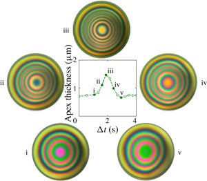
Figure 4 shows data collected from four experiments of binary silicone oil mixtures (1 cSt 0.1 vol%–20 cSt 99.9 vol%). Note that the experimentally measured film profile can deviate from the axisymmetric state, so the apex film thickness is defined as the maximum film thickness in the dimple region. During the initial second in the experiments, the motor moves the lower surface towards the upper interface and the film quickly thins due to the squeezing motion. The fast dynamics and the relatively large thickness of the film make it difficult to determine the apex film thickness through the interference patterns. For  $1~\text{s}<t^{\ast }<t_{stop}^{\ast }=3~\text{s}$, the film thickens (see dashed lines in figure 4a). After the motor stops, the film is allowed to evolve under the effects of evaporation. Thereafter, the apex film thickness fluctuates between 0.5 and
  $2~\unicode[STIX]{x03BC}\text{m}$ for many minutes. Apex film thickness oscillations are observed and the amplitudes of those oscillations vary between 0.2 and
  $1~\unicode[STIX]{x03BC}\text{m}$. The time it takes for one cycle of film thickness oscillation to occur in the experiment varies between 1 and 4 s. In the first 20 s of the experiments, the film stays nearly axisymmetric (figure 4b (i–v)); at longer times, there is significant asymmetry in the film profile (figure 4b (vi)).

Figure 4. Experimental film thickness evolution profiles. (a) Time evolution of the apex film thickness from four binary silicone oil experiments (1 cSt 0.1 vol% and 20 cSt 99.9 vol%). The open symbols mark the experimental apex film thickness and the dashed lines are there to guide the eye. The vertical dash-dot line represents the motor stop time ( $t_{stop}^{\ast }$) for all four experiments shown. The six filled symbols in experiment 1 correspond to (b) the six interference patterns at various time points. The diameter of each circular image corresponds to 0.5 mm. Panels (i)–(v) show the growth and decay for one oscillation cycle. Panel (vi) shows symmetry breaking at 20 s for that experiment; note the foot that developed in the two o’clock position. The reference colour map for the interference patterns is provided on the left-hand side of the plot.
Figure 5(a) shows the time evolution of apex film thickness,  $h(t,r=0)$, from three numerical simulations. The numerical simulations were performed at three initial concentrations:
  $\unicode[STIX]{x1D719}_{0}=0.001,0.003$ and
  $0.005$. The three conditions were chosen to examine the effect of initial concentration on the film thickness oscillation. The initial clearance and bubble radius were chosen to match the corresponding average values in the experiments. All material properties were matched to those of the materials used in the experiments. The motor stop time in the experiments was 3 s, while in the simulations the motor stop time was 1.5 s. During the motor movement period, the apex film thickness in the simulation grows apparently at three times the rate observed in the experiments. It was necessary to shorten the motor stop time in the simulations to avoid further overshoot. This overshoot of the film growth rate is a result of the global deformation of the bubble during approach, which is not included in the theory. In developing the lubrication theory, the far-field deformation of the lower surface is matched to the static shape of a pinned bubble. Whereas in the experiments, as the bubble moves closer to the top interface, it is flattened globally: evidence that the theory is under-accounting for the lower surface deformation. After the motor stops, the film in the simulations quickly thins, followed by oscillations in the film thickness. For all three simulations, the average apex film thickness is in the range of film thickness as observed across the four experiments. At
  $\unicode[STIX]{x1D719}_{0}=0.001$, the apex film thickness shows clear periodic oscillations, with a single dominant frequency of around 1 Hz (figure 5c). The simulation stops when the minimum film thickness becomes nanoscopic. At
  $\unicode[STIX]{x1D719}_{0}=0.003$, the film oscillation is first damped where the amplitude of the oscillation decreases from
  $1~\unicode[STIX]{x03BC}\text{m}$ to a small value. At longer times, the film oscillation then becomes more pronounced, with an oscillation amplitude growing again to
  $1~\unicode[STIX]{x03BC}\text{m}$. The dominant frequency for the apex film thickness oscillation is around 1.2 Hz (figure 5d). At
  $\unicode[STIX]{x1D719}_{0}=0.005$, the simulated film thickness oscillates only once after
  $t_{stop}^{\ast }$ and the subsequent oscillations are damped. No long-time oscillation was observed in this case.

Figure 5. Apex film thickness evolution profiles and their frequency spectra. (a) Time evolution of the apex film thickness from numerical simulations conducted at initial volume fractions of  $\unicode[STIX]{x1D719}_{0}=0.001,0.003$ and
  $0.005$. The vertical dash-dot line represents the motor stop time (
 $t_{stop}^{\ast }$). Other non-dimensional parameters corresponding to the three simulations are
  $\unicode[STIX]{x1D716}=0.067,{\mathcal{C}}{\mathcal{a}}=0.0156,{\mathcal{B}}{\mathcal{o}}=0.0678,{\mathcal{M}}{\mathcal{a}}=173,{\mathcal{M}}{\mathcal{a}}_{T}=255,{\mathcal{P}}{\mathcal{e}}=94,{\mathcal{P}}{\mathcal{e}}_{T}=1.15,{\mathcal{E}}{\mathcal{v}}=0.00728,\unicode[STIX]{x1D703}_{b}=130^{\circ }$. (b–d) Frequency spectra for selected apex film thickness evolution profiles in figure 4(a) and panel (a). The amplitude of the signal is normalized by the amplitude of the maximum signal.
The oscillation frequencies in the experiments and the simulations are clearly different. In the experiments, the oscillations do not show a single dominant frequency (figure 5b shows an example frequency spectrum). For the simulations with sustained oscillations, there is clear periodicity in the oscillations (figure 5c,d). The difference may be caused by sources of noise in the experiments. For example, the disturbances in the evaporation rate can impose temporally and spatially dependent fluctuations to the film thickness. In addition, imperfect mixing in the binary silicone oil mixtures can lead to spatial concentration inhomogeneities that can shift the oscillatory states between the stable oscillatory state and the damped state. Despite the differences, the model does provide a mechanism for the spontaneous oscillations and allows for an estimate regarding the relative contributions from the solutal and the thermal Marangoni flows. Furthermore, we are presenting a free, nonlinear oscillator with physical relevance, and we will discuss how various experimental parameters may affect the oscillation frequency.
4.2 Oscillation mechanism
We introduce the modified surface tension ( $\bar{\unicode[STIX]{x1D70F}}$) to explain the mechanism behind the spontaneous oscillations:
 $$\begin{eqnarray}\bar{\unicode[STIX]{x1D70F}}\equiv \unicode[STIX]{x1D70F}-\unicode[STIX]{x1D70F}(t=0)=-\unicode[STIX]{x1D716}{\mathcal{C}}{\mathcal{a}}({\mathcal{M}}{\mathcal{a}}(\unicode[STIX]{x1D719}-\unicode[STIX]{x1D719}_{0})+{\mathcal{M}}{\mathcal{a}}_{T}\unicode[STIX]{x1D6E9}).\end{eqnarray}$$
 Throughout the process, the species with the lower surface tension evaporates across the top interface and  $\unicode[STIX]{x1D719}$ and
  $\unicode[STIX]{x1D6E9}$ decrease due to the coupled mass and heat transfer process. Thus, surface tension in the thin film will increase as a result of evaporation, i.e.
  $\bar{\unicode[STIX]{x1D70F}}>0$. The rate at which
  $\bar{\unicode[STIX]{x1D70F}}$ increases will vary across the film based on the relative rates of change in
  $\unicode[STIX]{x1D719}$ and
  $\unicode[STIX]{x1D6E9}$, which are coupled to film thickness and curvature.

Figure 6. Time evolution of interface positions (a–c), film thickness (d–f), surface tension (g–i), and difference between capillary and Marangoni pressure gradients (j–l) for a simulation that corresponds to  $\unicode[STIX]{x1D716}=0.067$,
  ${\mathcal{C}}{\mathcal{a}}=0.0156$,
  ${\mathcal{B}}{\mathcal{o}}=0.0678$,
  ${\mathcal{M}}{\mathcal{a}}=173$,
  ${\mathcal{M}}{\mathcal{a}}_{T}=255$,
  ${\mathcal{P}}{\mathcal{e}}=94$,
  ${\mathcal{P}}{\mathcal{e}}_{T}=1.15$,
  ${\mathcal{E}}{\mathcal{v}}=0.00728$,
  $\unicode[STIX]{x1D719}_{0}=0.001$ and
  $t_{stop}=1.5$ (corresponding to the
  $\unicode[STIX]{x1D719}_{0}=0.001$ case in figure 5a). The legend represents non-dimensional time and the grey arrows indicate increasing time. Panel (a,d,g,j) shows the dimple formation while the needle is moving upward. Panel (b,e,h,k) shows the first capillary discharge after the needle has stopped moving. Panel (c,f,i,l) shows the first film regeneration associated with the Marangoni flows.
Figure 6 shows simulation results for the first cycle of film thickness oscillation, the associated changes in  $\bar{\unicode[STIX]{x1D70F}}$ and the pressure gradients, for the
  $\unicode[STIX]{x1D719}_{0}=0.001$ case presented in figure 5(a). Before
  $t_{stop}$, the bubble moves towards the initially flat top interface, squeezing liquid away from the centreline into the bulk region, thereby creating a film whose thickness varies in the radial direction. The evaporative species volume fraction depletes faster in regions where the film is thinner; consequently, a surface tension gradient is established.
During  $0<t<1$, the minimum film thickness is at
  $r=0$, where the surface tension is largest. The established surface tension gradient draws liquid from the bulk towards the centreline, generating a Marangoni flow (
 $1<t<1.61$). Due to the inflow, the film thickness becomes non-monotonic in the radial direction, forming the so-called spontaneous dimple. The formation of the dimple leads to a change in the capillary pressure and the capillary pressure gradient:
 $$\begin{eqnarray}\frac{\unicode[STIX]{x2202}\bar{\mathscr{P}}_{{\mathcal{C}}{\mathcal{a}}}}{\unicode[STIX]{x2202}r}=-\frac{1}{4}\frac{\unicode[STIX]{x2202}}{\unicode[STIX]{x2202}r}\left(\frac{1}{r}\frac{\unicode[STIX]{x2202}}{\unicode[STIX]{x2202}r}\left(r\frac{\unicode[STIX]{x2202}h}{\unicode[STIX]{x2202}r}\right)\right).\end{eqnarray}$$
 Here  $(\unicode[STIX]{x2202}\bar{\mathscr{P}}_{{\mathcal{C}}{\mathcal{a}}}/\unicode[STIX]{x2202}r)$ is the dominant contributing term to the dynamic pressure gradient and its value is predominantly positive due to the gradient in the curvature. Balancing the capillary pressure gradient is the depth-averaged surface tension gradient (equation (3.10)):
 $$\begin{eqnarray}\frac{1}{\unicode[STIX]{x1D716}}\frac{1}{h}\frac{\unicode[STIX]{x2202}\bar{\unicode[STIX]{x1D70F}}}{\unicode[STIX]{x2202}r}=-\frac{{\mathcal{C}}{\mathcal{a}}}{h}\left({\mathcal{M}}{\mathcal{a}}\frac{\unicode[STIX]{x2202}\unicode[STIX]{x1D719}}{\unicode[STIX]{x2202}r}+{\mathcal{M}}{\mathcal{a}}_{T}\frac{\unicode[STIX]{x2202}\unicode[STIX]{x1D6E9}}{\unicode[STIX]{x2202}r}\right).\end{eqnarray}$$
From the radial distribution of the surface tension plot, it is evident that the surface tension gradient is predominantly negative. The difference between the two gradients will give a clear indication as to which is the key mechanism that is driving the flow (figure 6j–l). As the lower surface is forced towards the top surface, the surface tension gradient dominates over the capillary pressure gradient, indicated by the positive radial distribution of the pressure gradient difference.
Eventually the capillary pressure gradient becomes large enough to overcome the Marangoni forces and to dispel liquid from the centreline region into the bulk ( $1.61<t<1.86$, figure 6k,
  $t=1.70$). Because the film near the centreline is thin and the bubble small, gravitational drainage contributes very little as compared to the capillary discharge. After the discharge, the film near the centreline becomes flat and the capillary pressure gradient is again overcome by the surface tension gradient and the difference between the gradients again become positive. Furthermore, the discharge process also re-establishes the surface tension gradient because the centreline region again has the thinnest film and thus the fastest change in
  $\unicode[STIX]{x1D719}$ and
  $\unicode[STIX]{x1D6E9}$ – creating a high surface tension again near
  $r=0$.
Finally, with the new surface tension gradient, the combined solutal and thermal Marangoni flow will again draw liquid from the bulk (where surface tension is lower than that in the centreline region) into the centreline, thereby reducing the surface tension gradient, increasing the capillary pressure gradient and providing the conditions for another fluid discharge and subsequent inflow.
4.3 Relative contributions of solutal and thermal Marangoni flows
In this section, we examine the relative contributions of the solutal and thermal Marangoni flows by comparing the relative contributions of the concentration gradient and the temperature gradient to the overall surface tension gradient:
 $$\begin{eqnarray}\frac{\unicode[STIX]{x2202}\bar{\unicode[STIX]{x1D70F}}}{\unicode[STIX]{x2202}r}=-\unicode[STIX]{x1D716}{\mathcal{C}}{\mathcal{a}}\left({\mathcal{M}}{\mathcal{a}}\frac{\unicode[STIX]{x2202}\unicode[STIX]{x1D719}}{\unicode[STIX]{x2202}r}+{\mathcal{M}}{\mathcal{a}}_{T}\frac{\unicode[STIX]{x2202}\unicode[STIX]{x1D6E9}}{\unicode[STIX]{x2202}r}\right).\end{eqnarray}$$
 Shown in figure 7 are radial profiles of surface tension gradients at  $t=t_{stop}$ for three different initial concentrations that correspond to the simulations presented in figure 5(a). The motion of the motor rising is the initial transient behaviour that starts the subsequent oscillations. The time at which the motor stops is the starting point of the subsequent long-term behaviour, and thus we can gain insights about the system by examining the dynamic variables at
  $t_{stop}$.

Figure 7. Radial profiles of surface tension gradient and its components at  $t=t_{stop}$ for the three simulations shown in figure 5(a).
At  $\unicode[STIX]{x1D719}_{0}=0.001$, the maximum values for solutal and thermal gradients are similar in magnitude, signifying a near-equal contribution from the two sources. The two gradients have different radial shapes: the concentration gradient has a broad peak whereas the thermal gradient grows and decays more sharply. Thus, in this case, the presence of the thermal Marangoni flow significantly modifies the curvature of the film. At
  $\unicode[STIX]{x1D719}_{0}=0.003$, the maximum magnitude of the concentration gradient is greater than that of the thermal gradient. The maxima of the two gradients occur near
  $r=0.4$ and the thermal gradient at that point contributes to one-third of the overall surface tension gradient. At
  $\unicode[STIX]{x1D719}_{0}=0.005$, solutal Marangoni flow contributes roughly three-quarters of the overall Marangoni flow at the maxima. In the latter two cases, the presence of the thermal Marangoni flow serves to enhance the overall Marangoni flow, but it does not significantly affect the curvature of the film, as the radial profiles of the gradients are similar in shape. Comparing results across the three concentrations, the thermal Marangoni flow is not affected by the change in the initial concentration, whereas the solutal Marangoni flow scales with the initial concentration. As a result, the overall surface tension gradient increases as the initial concentration increases and the oscillator becomes more damped as the initial concentration increases.
4.4 Damped oscillators
We examine the nature of these oscillations by looking at the phase portraits of the dimple volume, whose motion describes the composite effect of the Marangoni flows, capillarity, gravity and evaporation. The dimple volume is defined as
 $$\begin{eqnarray}V=2\unicode[STIX]{x03C0}\int _{0}^{R}hr\,\text{d}r,\end{eqnarray}$$
 where  $R$ is the radial position of the minimum film thickness. For the three simulations presented in figure 5(a), we plot the dimple volume against its rate of change in time (figure 8). The colour represents non-dimensional time. At
  $\unicode[STIX]{x1D719}_{0}=0.001$, as the motor moves upward, a dimple forms and by
  $t=t_{stop}$ the dimple volume reaches a maximum of 0.003, after which the dimple continues to oscillate at a near-constant amplitude and frequency – evidenced by the constant trajectory on the phase portrait. At
  $\unicode[STIX]{x1D719}_{0}=0.003$, the oscillator first enters an attractor region (around
  $t=5$) then traverses to a repeller region (
 $t>10$) where the oscillation amplitude grows and then enters a stable orbit. At
  $\unicode[STIX]{x1D719}_{0}=0.005$, the dimple grows and only oscillates a few times before entering a damped, dynamic steady state where draining due to capillarity and gravity is balancing the regenerative Marangoni flow. Across the three simulations, the maximum dimple volume increases with concentration, because the dimple-generating Marangoni flow strengthens with initial concentration (figure 7).

Figure 8. Phase portraits of the dimple volume ( $V$) for the three simulations shown in figure 5(a). The colour represents non-dimensional time, as indicated by the colour bars.
4.5 Oscillation frequency
In the experiments, it is relatively easy to vary  $\unicode[STIX]{x1D719}_{0}$ and
  $t_{stop}$. In this section, we look at how these two parameters affect the behaviour of the oscillator. The nonlinear nature of the governing equations makes it prohibitive to derive specific frequency scalings with respect to the parameter space. In this section, we focus on how the experimentally adjustable parameters affect the behaviour of the oscillator through the aid of numerical simulations (figure 9). With the previous set of simulations, it is clear that as
  $\unicode[STIX]{x1D719}_{0}$ increases, there is an increase in the Marangoni driving force and the system is damped more quickly. The simulations presented in this section all have sustained oscillations, which means that parameters such as the bubble radius and the initial apex clearance have been tuned to avoid cases where the system exhibits a dynamic steady state due to Marangoni damping.
When  $\unicode[STIX]{x1D719}_{0}$ is the only parameter that is varied, the amplitude of the dimple volume oscillation is nearly constant (figure 9a). At lower concentrations (
 $\unicode[STIX]{x1D719}_{0}=0.003$–
 $0.005$), the dominant frequency increases with concentration and the waveform of the dimple volume does not change significantly. The waveform changes shape when
  $\unicode[STIX]{x1D719}_{0}$ increases from 0.005 to 0.006. This change may be caused by a shift in the balance between the two contributing Marangoni flows for this specific set of simulation parameters. Figure 9(c) shows the period associated with the dominant frequency when each of the four simulations has reached steady oscillation, i.e. when the effect of the initial motor movement has worn off. As
  $\unicode[STIX]{x1D719}_{0}$ increases there is no clear trend in the period of the dimple volume oscillation. The period for the dimple to regenerate and to discharge can be further split into the Marangoni regeneration segment (from valley to peak,
  $1/f_{{\mathcal{M}}{\mathcal{a}}}$) and the capillary discharge segment (from peak to valley,
  $1/f_{{\mathcal{C}}{\mathcal{a}}}$). As the initial concentration increases, the time it takes for the dimple to regenerate decreases, because the overall Marangoni flow strength scales with
  $\unicode[STIX]{x1D719}_{0}$. On the other hand,
  $1/f_{{\mathcal{C}}{\mathcal{a}}}$ shows no clear relation to
  $\unicode[STIX]{x1D719}_{0}$.

Figure 9. (a,b) Time evolution of the dimple volumes (left-hand column) and their frequency spectra (right-hand column) at different  $\unicode[STIX]{x1D719}_{0}$ and
  $t_{stop}$. The amplitude of the Fourier signals are normalized by the amplitude of the maximum signal. The frequency is non-dimensionalized by
  $U/b$. (c,d) Corresponding steady oscillation time scales associated with the dominant frequency (
 $f_{D}$) and the time scales associated with Marangoni regeneration (
 $1/f_{{\mathcal{M}}{\mathcal{a}}}$) and capillary discharge (
 $1/f_{{\mathcal{C}}{\mathcal{a}}}$). (a) Variation in
  $\unicode[STIX]{x1D719}_{0}$. All other parameters are kept constant at
  $\unicode[STIX]{x1D716}=0.15$,
  ${\mathcal{C}}{\mathcal{a}}=0.00307$,
  ${\mathcal{B}}{\mathcal{o}}=0.0434$,
  ${\mathcal{M}}{\mathcal{a}}=389$,
  ${\mathcal{M}}{\mathcal{a}}_{T}=573$,
  ${\mathcal{P}}{\mathcal{e}}=50$,
  ${\mathcal{P}}{\mathcal{e}}_{T}=0.612$ and
  ${\mathcal{E}}{\mathcal{v}}=0.00728$. (b) Variation in
  $t_{stop}$. All other parameters are kept constant at
  $\unicode[STIX]{x1D716}=0.067$,
  ${\mathcal{C}}{\mathcal{a}}=0.0156$,
  ${\mathcal{B}}{\mathcal{o}}=0.0678$,
  ${\mathcal{M}}{\mathcal{a}}=173$,
  ${\mathcal{M}}{\mathcal{a}}_{T}=255$,
  ${\mathcal{P}}{\mathcal{e}}=93.8$,
  ${\mathcal{P}}{\mathcal{e}}_{T}=1.15$ and
  ${\mathcal{E}}{\mathcal{v}}=0.00728$. (c) Time scales for steady oscillations shown in (a). (d) Time scales for steady oscillations shown in (b).
When  $t_{stop}$ is the only increasing parameter, the amplitude of the oscillations increases because the duration of the motor movement is longer (figure 9b). When the motor is moving, Marangoni flows dominate and capillarity is not strong enough to discharge any liquid. This behaviour is reflected in the increase in apex film thickness during
  $1<t<t_{stop}$ and it is seen in both the simulations and the experiments. Thus, a longer time period for the initial inward flow will lead to a larger initial dimple and an increase in oscillation amplitude. The dominant frequency decreases with increasing
  $t_{stop}$ value, because a larger dimple volume takes longer to discharge. This trend is also reflected in the regeneration and discharge time scales (figure 9d). As the motor stop time increases, both processes take longer to complete, leading to the overall increase in the dominant period.
5 Conclusion
In this study, we present a spontaneously oscillatory thin-film system composed of a binary mixture of silicone oils with different surface tension and evaporation rates. Through the numerical solution of an axisymmetric lubrication model, we showed the mechanism behind the oscillatory behaviour. Evaporation of the lower-surface-tension component over an air bubble surface creates a surface tension gradient across the thin film. The ensuing Marangoni flow draws lower-surface-tension fluids to the centreline and in the process creates a dimple and diminishes the surface tension gradient. Eventually, capillary pressure overwhelms the Marangoni forces, since the surface tension gradient is diminishing, leading to a capillary discharge and the oscillation.
The set of nonlinear partial differential equations thus demonstrates an oscillatory solution in the absence of an external oscillatory driving force. In the experiments and the simulations, the amplitudes of the apex film thickness oscillations are similar; however, the frequencies do not agree. The disagreement may be caused by disturbances and symmetry breaking, as witnessed in the experiments. By probing a small parameter space, we found that the nonlinear oscillator is more prone to be damped with increasing solvent concentration, because the Marangoni flow grows stronger with increasing solvent concentration. We also find that the oscillation frequency is dependent on the motor stop time, which sets the amplitude of the dimple volume for subsequent oscillations. As a natural step forward, we are building a two-dimensional model to capture the non-axisymmetric effects that are observed in the experiments.
Acknowledgements
This project is funded by Beijing Welltrailing Science and Technology Company. X.S. thanks the following: Dr J. M. Barakat for his guidance on the development of the theoretical model, M. Rodríguez-Hakim for her generous help in disturbance control in the experiments and V. Chandran Suja for teaching the use of the DFI and the subsequent data processing.
Declaration of interests
The authors report no conflict of interest.
Appendix A
A.1 Derivation of the governing equations
Define the shape functions for the top and the bottom interfaces to be  $f_{1}=z-h_{1}$ and
  $f_{2}=z-h_{2}$. Let the surface normal vectors point from the gas phase into the liquid phase. Then the unit normals and their components on the two surfaces are
 $$\begin{eqnarray}\boldsymbol{n}_{1}=-\frac{\unicode[STIX]{x1D735}f_{1}}{||\unicode[STIX]{x1D735}f_{1}||},\quad {\boldsymbol{n}_{1}}_{r}=+\frac{1}{S_{1}}\frac{\unicode[STIX]{x2202}h_{1}}{\unicode[STIX]{x2202}r},\quad {\boldsymbol{n}_{1}}_{z}=-\frac{1}{S_{1}},\quad S_{1}=\sqrt{1+\left(\frac{\unicode[STIX]{x2202}h_{1}}{\unicode[STIX]{x2202}r}\right)^{2}};\end{eqnarray}$$
 $$\begin{eqnarray}\boldsymbol{n}_{2}=+\frac{\unicode[STIX]{x1D735}f_{2}}{||\unicode[STIX]{x1D735}f_{2}||},\quad {\boldsymbol{n}_{2}}_{r}=-\frac{1}{S_{2}}\frac{\unicode[STIX]{x2202}h_{2}}{\unicode[STIX]{x2202}r},\quad {\boldsymbol{n}_{2}}_{z}=+\frac{1}{S_{2}},\quad S_{2}=\sqrt{1+\left(\frac{\unicode[STIX]{x2202}h_{2}}{\unicode[STIX]{x2202}r}\right)^{2}}.\end{eqnarray}$$
Based on the proposed scaling, we have the following set of non-dimensional equations. Mass and momentum balances in the Stokes regime are
 $$\begin{eqnarray}\displaystyle & \displaystyle \frac{\unicode[STIX]{x2202}v_{z}}{\unicode[STIX]{x2202}z}+\frac{1}{r}\frac{\unicode[STIX]{x2202}}{\unicode[STIX]{x2202}r}\left(rv_{r}\right)=0, & \displaystyle\end{eqnarray}$$
 $$\begin{eqnarray}\displaystyle & \displaystyle \frac{\unicode[STIX]{x2202}P}{\unicode[STIX]{x2202}z}=\unicode[STIX]{x1D716}\frac{\unicode[STIX]{x2202}^{2}v_{z}}{\unicode[STIX]{x2202}z^{2}}+\unicode[STIX]{x1D716}^{2}\frac{1}{r}\frac{\unicode[STIX]{x2202}}{\unicode[STIX]{x2202}r}\left(r\frac{\unicode[STIX]{x2202}v_{z}}{\unicode[STIX]{x2202}r}\right)-\frac{{\mathcal{B}}{\mathcal{o}}}{{\mathcal{C}}{\mathcal{a}}}, & \displaystyle\end{eqnarray}$$
 $$\begin{eqnarray}\displaystyle & \displaystyle \frac{\unicode[STIX]{x2202}P}{\unicode[STIX]{x2202}r}=\frac{\unicode[STIX]{x2202}^{2}v_{r}}{\unicode[STIX]{x2202}z^{2}}+\unicode[STIX]{x1D716}\frac{\unicode[STIX]{x2202}}{\unicode[STIX]{x2202}r}\left(\frac{1}{r}\frac{\unicode[STIX]{x2202}}{\unicode[STIX]{x2202}r}(rv_{r})\right); & \displaystyle\end{eqnarray}$$
and the associated kinematic boundary conditions are
 $$\begin{eqnarray}\displaystyle & \displaystyle \frac{\unicode[STIX]{x2202}h_{1}}{\unicode[STIX]{x2202}t}-v_{z}\big|_{h_{1}}+\frac{\unicode[STIX]{x2202}h_{1}}{\unicode[STIX]{x2202}r}\cdot v_{r}\big|_{h_{1}}=-S_{1}{\mathcal{E}}{\mathcal{v}}\unicode[STIX]{x1D719}, & \displaystyle\end{eqnarray}$$
 $$\begin{eqnarray}\displaystyle & \displaystyle \frac{\unicode[STIX]{x2202}h_{2}}{\unicode[STIX]{x2202}t}-v_{z}\big|_{h_{2}}+\frac{\unicode[STIX]{x2202}h_{2}}{\unicode[STIX]{x2202}r}\cdot v_{r}\big|_{h_{2}}=0. & \displaystyle\end{eqnarray}$$
Normal stress balances on the two surfaces are
 $$\begin{eqnarray}\displaystyle & & \displaystyle -P+\unicode[STIX]{x1D716}\frac{2}{S_{1}^{2}}\left[\frac{\unicode[STIX]{x2202}v_{z}}{\unicode[STIX]{x2202}z}-\frac{\unicode[STIX]{x2202}h_{1}}{\unicode[STIX]{x2202}r}\left(\unicode[STIX]{x1D716}\frac{\unicode[STIX]{x2202}v_{z}}{\unicode[STIX]{x2202}r}+\frac{\unicode[STIX]{x2202}v_{r}}{\unicode[STIX]{x2202}z}\right)+\unicode[STIX]{x1D716}\left(\frac{\unicode[STIX]{x2202}h_{1}}{\unicode[STIX]{x2202}r}\right)^{2}\frac{\unicode[STIX]{x2202}v_{r}}{\unicode[STIX]{x2202}r}\right]\nonumber\\ \displaystyle & & \displaystyle \quad =+\left(1-\unicode[STIX]{x1D716}{\mathcal{M}}{\mathcal{a}}\unicode[STIX]{x1D719}-\unicode[STIX]{x1D716}{\mathcal{M}}{\mathcal{a}}_{T}\unicode[STIX]{x1D6E9}\right)\left(\frac{1}{r}\frac{\unicode[STIX]{x2202}}{\unicode[STIX]{x2202}r}\left(\frac{r}{S_{1}}\frac{\unicode[STIX]{x2202}h_{1}}{\unicode[STIX]{x2202}r}\right)\right),\end{eqnarray}$$
 $$\begin{eqnarray}\displaystyle & & \displaystyle -P+\unicode[STIX]{x1D716}\frac{2}{S_{2}^{2}}\left[\frac{\unicode[STIX]{x2202}v_{z}}{\unicode[STIX]{x2202}z}-\frac{\unicode[STIX]{x2202}h_{2}}{\unicode[STIX]{x2202}r}\left(\unicode[STIX]{x1D716}\frac{\unicode[STIX]{x2202}v_{z}}{\unicode[STIX]{x2202}r}+\frac{\unicode[STIX]{x2202}v_{r}}{\unicode[STIX]{x2202}z}\right)+\unicode[STIX]{x1D716}\left(\frac{\unicode[STIX]{x2202}h_{2}}{\unicode[STIX]{x2202}r}\right)^{2}\frac{\unicode[STIX]{x2202}v_{r}}{\unicode[STIX]{x2202}r}\right]\nonumber\\ \displaystyle & & \displaystyle \quad =-\left(1-\unicode[STIX]{x1D716}{\mathcal{M}}{\mathcal{a}}\unicode[STIX]{x1D719}-\unicode[STIX]{x1D716}{\mathcal{M}}{\mathcal{a}}_{T}\unicode[STIX]{x1D6E9}\right)\left(\frac{1}{r}\frac{\unicode[STIX]{x2202}}{\unicode[STIX]{x2202}r}\left(\frac{r}{S_{2}}\frac{\unicode[STIX]{x2202}h_{2}}{\unicode[STIX]{x2202}r}\right)\right)-2;\end{eqnarray}$$
and tangential stress balances are
 $$\begin{eqnarray}\displaystyle & & \displaystyle \frac{\unicode[STIX]{x2202}v_{r}}{\unicode[STIX]{x2202}z}+\unicode[STIX]{x1D716}\left[\frac{\unicode[STIX]{x2202}v_{z}}{\unicode[STIX]{x2202}r}+2\frac{\unicode[STIX]{x2202}h_{1}}{\unicode[STIX]{x2202}r}\left(\frac{\unicode[STIX]{x2202}v_{z}}{\unicode[STIX]{x2202}z}-\frac{\unicode[STIX]{x2202}v_{r}}{\unicode[STIX]{x2202}r}\right)-\left(\frac{\unicode[STIX]{x2202}h_{1}}{\unicode[STIX]{x2202}r}\right)^{2}\frac{\unicode[STIX]{x2202}v_{r}}{\unicode[STIX]{x2202}z}\right]+O(\unicode[STIX]{x1D716}^{2})\nonumber\\ \displaystyle & & \displaystyle \quad =\left(-{\mathcal{M}}{\mathcal{a}}\frac{\unicode[STIX]{x2202}\unicode[STIX]{x1D719}}{\unicode[STIX]{x2202}r}-{\mathcal{M}}{\mathcal{a}}_{T}\frac{\unicode[STIX]{x2202}\unicode[STIX]{x1D6E9}}{\unicode[STIX]{x2202}r}\right)\left(1+\frac{\unicode[STIX]{x1D716}}{2}\left(\frac{\unicode[STIX]{x2202}h_{1}}{\unicode[STIX]{x2202}r}\right)^{2}+O(\unicode[STIX]{x1D716}^{2})\right),\end{eqnarray}$$
 $$\begin{eqnarray}\displaystyle & & \displaystyle \frac{\unicode[STIX]{x2202}v_{r}}{\unicode[STIX]{x2202}z}+\unicode[STIX]{x1D716}\left[\frac{\unicode[STIX]{x2202}v_{z}}{\unicode[STIX]{x2202}r}+2\frac{\unicode[STIX]{x2202}h_{2}}{\unicode[STIX]{x2202}r}\left(\frac{\unicode[STIX]{x2202}v_{z}}{\unicode[STIX]{x2202}z}-\frac{\unicode[STIX]{x2202}v_{r}}{\unicode[STIX]{x2202}r}\right)-\left(\frac{\unicode[STIX]{x2202}h_{2}}{\unicode[STIX]{x2202}r}\right)^{2}\frac{\unicode[STIX]{x2202}v_{r}}{\unicode[STIX]{x2202}z}\right]+O(\unicode[STIX]{x1D716}^{2})\nonumber\\ \displaystyle & & \displaystyle \quad =\left(+{\mathcal{M}}{\mathcal{a}}\frac{\unicode[STIX]{x2202}\unicode[STIX]{x1D719}}{\unicode[STIX]{x2202}r}+{\mathcal{M}}{\mathcal{a}}_{T}\frac{\unicode[STIX]{x2202}\unicode[STIX]{x1D6E9}}{\unicode[STIX]{x2202}r}\right)\left(1+\frac{\unicode[STIX]{x1D716}}{2}\left(\frac{\unicode[STIX]{x2202}h_{2}}{\unicode[STIX]{x2202}r}\right)^{2}+O(\unicode[STIX]{x1D716}^{2})\right).\end{eqnarray}$$
We assume that mass and energy losses only happen through the top interface because the dead volume is small. As such, the mass balance for the solute species and the associated boundary conditions are
 $$\begin{eqnarray}\displaystyle & \displaystyle \frac{\unicode[STIX]{x2202}\unicode[STIX]{x1D719}}{\unicode[STIX]{x2202}t}+v_{r}\frac{\unicode[STIX]{x2202}\unicode[STIX]{x1D719}}{\unicode[STIX]{x2202}r}+v_{z}\frac{\unicode[STIX]{x2202}\unicode[STIX]{x1D719}}{\unicode[STIX]{x2202}z}=\frac{1}{{\mathcal{P}}{\mathcal{e}}}\left(\frac{1}{\unicode[STIX]{x1D716}}\frac{\unicode[STIX]{x2202}^{2}\unicode[STIX]{x1D719}}{\unicode[STIX]{x2202}z^{2}}+\frac{1}{r}\frac{\unicode[STIX]{x2202}}{\unicode[STIX]{x2202}r}\left(r\frac{\unicode[STIX]{x2202}\unicode[STIX]{x1D719}}{\unicode[STIX]{x2202}r}\right)\right), & \displaystyle\end{eqnarray}$$
 $$\begin{eqnarray}\displaystyle & \displaystyle \frac{1}{{\mathcal{P}}{\mathcal{e}}}\frac{1}{S_{1}}\left(\unicode[STIX]{x1D716}\frac{\unicode[STIX]{x2202}h_{1}}{\unicode[STIX]{x2202}r}\frac{\unicode[STIX]{x2202}\unicode[STIX]{x1D719}}{\unicode[STIX]{x2202}r}\bigg|_{h_{1}}-\frac{\unicode[STIX]{x2202}\unicode[STIX]{x1D719}}{\unicode[STIX]{x2202}z}\bigg|_{h_{1}}\right)=\unicode[STIX]{x1D716}{\mathcal{E}}{\mathcal{v}}\unicode[STIX]{x1D719}(1-\unicode[STIX]{x1D719})\bigg|_{h_{1}}, & \displaystyle\end{eqnarray}$$
 $$\begin{eqnarray}\displaystyle & \displaystyle \unicode[STIX]{x1D716}\frac{\unicode[STIX]{x2202}h_{2}}{\unicode[STIX]{x2202}r}\frac{\unicode[STIX]{x2202}\unicode[STIX]{x1D719}}{\unicode[STIX]{x2202}r}\bigg|_{h_{2}}=\frac{\unicode[STIX]{x2202}\unicode[STIX]{x1D719}}{\unicode[STIX]{x2202}z}\bigg|_{h_{2}}. & \displaystyle\end{eqnarray}$$
The energy balance and heat flux conditions are
 $$\begin{eqnarray}\displaystyle & \displaystyle \frac{\unicode[STIX]{x2202}\unicode[STIX]{x1D6E9}}{\unicode[STIX]{x2202}t}+v_{r}\frac{\unicode[STIX]{x2202}\unicode[STIX]{x1D6E9}}{\unicode[STIX]{x2202}r}+v_{z}\frac{\unicode[STIX]{x2202}\unicode[STIX]{x1D6E9}}{\unicode[STIX]{x2202}z}=\frac{1}{{\mathcal{P}}{\mathcal{e}}_{T}}\left(\frac{1}{\unicode[STIX]{x1D716}}\frac{\unicode[STIX]{x2202}^{2}\unicode[STIX]{x1D6E9}}{\unicode[STIX]{x2202}z^{2}}+\frac{1}{r}\frac{\unicode[STIX]{x2202}}{\unicode[STIX]{x2202}r}\left(r\frac{\unicode[STIX]{x2202}\unicode[STIX]{x1D6E9}}{\unicode[STIX]{x2202}r}\right)\right), & \displaystyle\end{eqnarray}$$
 $$\begin{eqnarray}\displaystyle & \displaystyle \frac{1}{{\mathcal{P}}{\mathcal{e}}_{T}}\frac{1}{S_{1}}\left(\unicode[STIX]{x1D716}\frac{\unicode[STIX]{x2202}h_{1}}{\unicode[STIX]{x2202}r}\frac{\unicode[STIX]{x2202}\unicode[STIX]{x1D6E9}}{\unicode[STIX]{x2202}r}\bigg|_{h_{1}}-\frac{\unicode[STIX]{x2202}\unicode[STIX]{x1D6E9}}{\unicode[STIX]{x2202}z}\bigg|_{h_{1}}\right)=\unicode[STIX]{x1D716}{\mathcal{E}}{\mathcal{v}}\unicode[STIX]{x1D719}\bigg|_{h_{1}}, & \displaystyle\end{eqnarray}$$
 $$\begin{eqnarray}\displaystyle & \displaystyle \unicode[STIX]{x1D716}\frac{\unicode[STIX]{x2202}h_{2}}{\unicode[STIX]{x2202}r}\frac{\unicode[STIX]{x2202}\unicode[STIX]{x1D6E9}}{\unicode[STIX]{x2202}r}\bigg|_{h_{2}}=\frac{\unicode[STIX]{x2202}\unicode[STIX]{x1D6E9}}{\unicode[STIX]{x2202}z}\bigg|_{h_{2}}. & \displaystyle\end{eqnarray}$$
 Now expand all variables in  $\unicode[STIX]{x1D716}$:
  $\unicode[STIX]{x1D713}=\unicode[STIX]{x1D713}^{0}+\unicode[STIX]{x1D716}\unicode[STIX]{x1D713}^{(1)}+\unicode[STIX]{x1D716}^{2}\unicode[STIX]{x1D713}^{2}+\cdots \,$. Then extract the
  $O(1)$ and
  $O(\unicode[STIX]{x1D716})$ equations from the above set of equations. At
  $O(1)$, integrate the mass conservation equation with respect to
  $z$ and apply the kinematic boundary conditions on the two surfaces to get
 $$\begin{eqnarray}\frac{\unicode[STIX]{x2202}h^{(0)}}{\unicode[STIX]{x2202}t}+\frac{1}{r}\frac{\unicode[STIX]{x2202}}{\unicode[STIX]{x2202}r}\left(rh^{(0)}\left<v\right>^{(0)}\right)+{\mathcal{E}}{\mathcal{v}}\unicode[STIX]{x1D719}^{(0)}=0,\end{eqnarray}$$
 where  $\left<v\right>^{(0)}\equiv (1/h^{(0)})\int _{h_{2}^{(0)}}^{h_{1}^{(0)}}v_{r}^{(0)}\,\text{d}z$. A similar derivation process is applied to the species and energy balance equations. Specifically, the
  $O(1)$ governing equations and boundary conditions for
  $\unicode[STIX]{x1D719}$ are
 $$\begin{eqnarray}\frac{\unicode[STIX]{x2202}^{2}\unicode[STIX]{x1D719}^{(0)}}{\unicode[STIX]{x2202}z^{2}}=0\quad \text{and}\quad \frac{\unicode[STIX]{x2202}\unicode[STIX]{x1D719}^{(0)}}{\unicode[STIX]{x2202}z}\bigg|_{h_{1}^{(0)},h_{2}^{(0)}}=0\end{eqnarray}$$
and it follows that
 $$\begin{eqnarray}\unicode[STIX]{x1D719}^{(0)}=\unicode[STIX]{x1D719}^{(0)}(t,r).\end{eqnarray}$$
 Integrate the  $O(\unicode[STIX]{x1D716})$ solute governing equation with respect to
  $z$ and apply the above conclusion to get
 $$\begin{eqnarray}h^{(0)}\frac{\unicode[STIX]{x2202}\unicode[STIX]{x1D719}^{(0)}}{\unicode[STIX]{x2202}t}+\frac{\unicode[STIX]{x2202}\unicode[STIX]{x1D719}^{(0)}}{\unicode[STIX]{x2202}r}\int _{h_{2}^{(0)}}^{h_{1}^{(0)}}v_{r}^{(0)}\,\text{d}z-\frac{h^{(0)}}{{\mathcal{P}}{\mathcal{e}}}\frac{1}{r}\frac{\unicode[STIX]{x2202}}{\unicode[STIX]{x2202}r}\left(r\frac{\unicode[STIX]{x2202}\unicode[STIX]{x1D719}^{(0)}}{\unicode[STIX]{x2202}r}\right)=\frac{1}{{\mathcal{P}}{\mathcal{e}}}\left(\frac{\unicode[STIX]{x2202}\unicode[STIX]{x1D719}^{(1)}}{\unicode[STIX]{x2202}z}\bigg|_{h_{1}^{(0)}}-\frac{\unicode[STIX]{x2202}\unicode[STIX]{x1D719}^{(1)}}{\unicode[STIX]{x2202}z}\bigg|_{h_{2}^{(0)}}\right).\end{eqnarray}$$
The boundary conditions on the two surfaces yield the following relation:
 $$\begin{eqnarray}\frac{\unicode[STIX]{x2202}\unicode[STIX]{x1D719}^{(1)}}{\unicode[STIX]{x2202}z}\bigg|_{h_{1}^{(0)}}-\frac{\unicode[STIX]{x2202}\unicode[STIX]{x1D719}^{(1)}}{\unicode[STIX]{x2202}z}\bigg|_{h_{2}^{(0)}}=-{\mathcal{P}}{\mathcal{e}}{\mathcal{E}}{\mathcal{v}}\unicode[STIX]{x1D719}^{(0)}(1-\unicode[STIX]{x1D719}^{(0)})+\frac{\unicode[STIX]{x2202}h^{(0)}}{\unicode[STIX]{x2202}r}\frac{\unicode[STIX]{x2202}\unicode[STIX]{x1D719}^{(0)}}{\unicode[STIX]{x2202}r}.\end{eqnarray}$$
 Combining the above two equations leads to the governing equation for  $\unicode[STIX]{x1D719}^{(0)}$:
 $$\begin{eqnarray}\frac{\unicode[STIX]{x2202}\unicode[STIX]{x1D719}^{(0)}}{\unicode[STIX]{x2202}t}+\left<v\right>^{(0)}\frac{\unicode[STIX]{x2202}\unicode[STIX]{x1D719}^{(0)}}{\unicode[STIX]{x2202}r}-\frac{1}{{\mathcal{P}}{\mathcal{e}}}\frac{1}{r}\frac{\unicode[STIX]{x2202}}{\unicode[STIX]{x2202}r}\left(r\frac{\unicode[STIX]{x2202}\unicode[STIX]{x1D719}^{(0)}}{\unicode[STIX]{x2202}r}\right)-\frac{1}{{\mathcal{P}}{\mathcal{e}}}\frac{1}{h^{(0)}}\frac{\unicode[STIX]{x2202}h^{(0)}}{\unicode[STIX]{x2202}r}\frac{\unicode[STIX]{x2202}\unicode[STIX]{x1D719}^{(0)}}{\unicode[STIX]{x2202}r}=-\frac{{\mathcal{E}}{\mathcal{v}}\unicode[STIX]{x1D719}^{(0)}(1-\unicode[STIX]{x1D719}^{(0)})}{h^{(0)}}.\end{eqnarray}$$
Taking advantage of the similarities between the mass transport equation and the energy transport equation, we get
 $$\begin{eqnarray}\frac{\unicode[STIX]{x2202}\unicode[STIX]{x1D6E9}^{(0)}}{\unicode[STIX]{x2202}t}+\left<v\right>^{(0)}\frac{\unicode[STIX]{x2202}\unicode[STIX]{x1D6E9}^{(0)}}{\unicode[STIX]{x2202}r}-\frac{1}{{\mathcal{P}}{\mathcal{e}}_{T}}\frac{1}{r}\frac{\unicode[STIX]{x2202}}{\unicode[STIX]{x2202}r}\left(r\frac{\unicode[STIX]{x2202}\unicode[STIX]{x1D6E9}^{(0)}}{\unicode[STIX]{x2202}r}\right)-\frac{1}{{\mathcal{P}}{\mathcal{e}}_{T}}\frac{1}{h^{(0)}}\frac{\unicode[STIX]{x2202}h^{(0)}}{\unicode[STIX]{x2202}r}\frac{\unicode[STIX]{x2202}\unicode[STIX]{x1D6E9}^{(0)}}{\unicode[STIX]{x2202}r}=-\frac{{\mathcal{E}}{\mathcal{v}}\unicode[STIX]{x1D719}^{(0)}}{h^{(0)}}.\end{eqnarray}$$
 After rearranging the mass, species and energy balance equation, we are left with the stress balances. From the  $z$-direction momentum balance equation, we get
 $$\begin{eqnarray}\frac{\unicode[STIX]{x2202}P^{(0)}}{\unicode[STIX]{x2202}z}=-\frac{{\mathcal{B}}{\mathcal{o}}}{{\mathcal{C}}{\mathcal{a}}}\Rightarrow P^{(0)}=-\frac{{\mathcal{B}}{\mathcal{o}}}{{\mathcal{C}}{\mathcal{a}}}z+\mathscr{P}^{(0)}(t,r).\end{eqnarray}$$
Apply the above relation to the normal stress balances on the top interface to get
 $$\begin{eqnarray}\frac{1}{r}\frac{\unicode[STIX]{x2202}}{\unicode[STIX]{x2202}r}\left(r\frac{\unicode[STIX]{x2202}h_{1}^{(0)}}{\unicode[STIX]{x2202}r}\right)-{\mathcal{B}}{\mathcal{o}}h_{1}^{(0)}={\mathcal{B}}{\mathcal{o}}{\mathcal{E}}{\mathcal{v}}\unicode[STIX]{x1D719}_{0}t-\mathscr{P}^{(0)}.\end{eqnarray}$$
Finally for the tangential stress balances, on the two surfaces we have
 $$\begin{eqnarray}\left.\begin{array}{@{}c@{}}\displaystyle \frac{\unicode[STIX]{x2202}v_{r}^{(0)}}{\unicode[STIX]{x2202}z}\bigg|_{h_{1}^{(0)}}=\left(-{\mathcal{M}}{\mathcal{a}}\frac{\unicode[STIX]{x2202}\unicode[STIX]{x1D719}^{(0)}}{\unicode[STIX]{x2202}r}-{\mathcal{M}}{\mathcal{a}}_{T}\frac{\unicode[STIX]{x2202}\unicode[STIX]{x1D6E9}^{(0)}}{\unicode[STIX]{x2202}r}\right)\bigg|_{h_{1}^{(0)}},\\ \displaystyle \frac{\unicode[STIX]{x2202}v_{r}^{(0)}}{\unicode[STIX]{x2202}z}\bigg|_{h_{2}^{(0)}}=\left(+{\mathcal{M}}{\mathcal{a}}\frac{\unicode[STIX]{x2202}\unicode[STIX]{x1D719}^{(0)}}{\unicode[STIX]{x2202}r}+{\mathcal{M}}{\mathcal{a}}_{T}\frac{\unicode[STIX]{x2202}\unicode[STIX]{x1D6E9}^{(0)}}{\unicode[STIX]{x2202}r}\right)\bigg|_{h_{2}^{(0)}}.\end{array}\right\}\end{eqnarray}$$
 Integrate the  $r$-direction momentum balance equation with respect to
  $z$, apply the two tangential stress balances and realize that
  $(\unicode[STIX]{x2202}P^{(0)}/\unicode[STIX]{x2202}r)=(\unicode[STIX]{x2202}\mathscr{P}^{(0)}/\unicode[STIX]{x2202}r)$:
 $$\begin{eqnarray}h^{(0)}\frac{\unicode[STIX]{x2202}\mathscr{P}^{(0)}}{\unicode[STIX]{x2202}r}=-2\left({\mathcal{M}}{\mathcal{a}}\frac{\unicode[STIX]{x2202}\unicode[STIX]{x1D719}^{(0)}}{\unicode[STIX]{x2202}r}+{\mathcal{M}}{\mathcal{a}}_{T}\frac{\unicode[STIX]{x2202}\unicode[STIX]{x1D6E9}^{(0)}}{\unicode[STIX]{x2202}r}\right).\end{eqnarray}$$
 To summarize, at  $O(1)$ we have the following set of governing equations:
 $$\begin{eqnarray}\frac{\unicode[STIX]{x2202}h^{(0)}}{\unicode[STIX]{x2202}t}+\frac{1}{r}\frac{\unicode[STIX]{x2202}}{\unicode[STIX]{x2202}r}\left(rh^{(0)}\left<v\right>^{(0)}\right)+{\mathcal{E}}{\mathcal{v}}\unicode[STIX]{x1D719}^{(0)}=0,\end{eqnarray}$$
 $$\begin{eqnarray}\displaystyle & & \displaystyle \frac{\unicode[STIX]{x2202}\unicode[STIX]{x1D719}^{(0)}}{\unicode[STIX]{x2202}t}+\left<v\right>^{(0)}\frac{\unicode[STIX]{x2202}\unicode[STIX]{x1D719}^{(0)}}{\unicode[STIX]{x2202}r}-\frac{1}{{\mathcal{P}}{\mathcal{e}}}\frac{1}{h^{(0)}}\frac{\unicode[STIX]{x2202}h^{(0)}}{\unicode[STIX]{x2202}r}\frac{\unicode[STIX]{x2202}\unicode[STIX]{x1D719}^{(0)}}{\unicode[STIX]{x2202}r}-\frac{1}{{\mathcal{P}}{\mathcal{e}}}\frac{1}{r}\frac{\unicode[STIX]{x2202}}{\unicode[STIX]{x2202}r}\left(r\frac{\unicode[STIX]{x2202}\unicode[STIX]{x1D719}^{(0)}}{\unicode[STIX]{x2202}r}\right)\nonumber\\ \displaystyle & & \displaystyle \quad =-\frac{{\mathcal{E}}{\mathcal{v}}}{h^{(0)}}\unicode[STIX]{x1D719}^{(0)}(1-\unicode[STIX]{x1D719}^{(0)}),\end{eqnarray}$$
 $$\begin{eqnarray}\displaystyle & \displaystyle \frac{\unicode[STIX]{x2202}\unicode[STIX]{x1D6E9}^{(0)}}{\unicode[STIX]{x2202}t}+\left<v\right>^{(0)}\frac{\unicode[STIX]{x2202}\unicode[STIX]{x1D6E9}^{(0)}}{\unicode[STIX]{x2202}r}-\frac{1}{{\mathcal{P}}{\mathcal{e}}_{T}}\frac{1}{r}\frac{\unicode[STIX]{x2202}}{\unicode[STIX]{x2202}r}\left(r\frac{\unicode[STIX]{x2202}\unicode[STIX]{x1D6E9}^{(0)}}{\unicode[STIX]{x2202}r}\right)-\frac{1}{{\mathcal{P}}{\mathcal{e}}_{T}}\frac{1}{h^{(0)}}\frac{\unicode[STIX]{x2202}h^{(0)}}{\unicode[STIX]{x2202}r}\frac{\unicode[STIX]{x2202}\unicode[STIX]{x1D6E9}^{(0)}}{\unicode[STIX]{x2202}r}=-\frac{{\mathcal{E}}{\mathcal{v}}\unicode[STIX]{x1D719}^{(0)}}{h^{(0)}},\qquad & \displaystyle\end{eqnarray}$$
 $$\begin{eqnarray}\displaystyle & \displaystyle \frac{1}{r}\frac{\unicode[STIX]{x2202}}{\unicode[STIX]{x2202}r}\left(r\frac{\unicode[STIX]{x2202}h_{1}^{(0)}}{\unicode[STIX]{x2202}r}\right)-{\mathcal{B}}{\mathcal{o}}h_{1}^{(0)}={\mathcal{B}}{\mathcal{o}}{\mathcal{E}}{\mathcal{v}}\unicode[STIX]{x1D719}_{0}t-\mathscr{P}^{(0)}, & \displaystyle\end{eqnarray}$$
 $$\begin{eqnarray}\displaystyle & \displaystyle \frac{\unicode[STIX]{x2202}\mathscr{P}^{(0)}}{\unicode[STIX]{x2202}r}=-\frac{2{\mathcal{M}}{\mathcal{a}}}{h^{(0)}}\frac{\unicode[STIX]{x2202}\unicode[STIX]{x1D719}^{(0)}}{\unicode[STIX]{x2202}r}-\frac{2{\mathcal{M}}{\mathcal{a}}_{T}}{h^{(0)}}\frac{\unicode[STIX]{x2202}\unicode[STIX]{x1D6E9}^{(0)}}{\unicode[STIX]{x2202}r}. & \displaystyle\end{eqnarray}$$
 We include the  $O(\unicode[STIX]{x1D716})$ equations to regularize the governing equations in the absence of Marangoni flows. In developing the
  $O(\unicode[STIX]{x1D716})$ equations, we neglect terms that are of the order of
  ${\mathcal{M}}{\mathcal{a}}\unicode[STIX]{x1D719}_{0}$ and
  ${\mathcal{M}}{\mathcal{a}}_{T}$, leading to the following approximations:
 $$\begin{eqnarray}v_{r}^{(0)}\approx \left<v\right>^{(0)},\quad \frac{\unicode[STIX]{x2202}v_{r}^{(0)}}{\unicode[STIX]{x2202}z}\approx 0,\quad \frac{\unicode[STIX]{x2202}v_{r}^{(0)}}{\unicode[STIX]{x2202}r}\approx \frac{\unicode[STIX]{x2202}\left<v\right>^{(0)}}{\unicode[STIX]{x2202}r},\end{eqnarray}$$
 $$\begin{eqnarray}\frac{1}{r}\frac{\unicode[STIX]{x2202}}{\unicode[STIX]{x2202}r}\left(rv_{r}^{(0)}\right)=-\frac{\unicode[STIX]{x2202}v_{z}^{(0)}}{\unicode[STIX]{x2202}z}\approx \frac{1}{r}\frac{\unicode[STIX]{x2202}}{\unicode[STIX]{x2202}r}\left(r\left<v\right>^{(0)}\right),\quad \frac{\unicode[STIX]{x2202}v_{z}^{(0)}}{\unicode[STIX]{x2202}r}\approx -z\frac{\unicode[STIX]{x2202}}{\unicode[STIX]{x2202}r}\left(\frac{1}{r}\frac{\unicode[STIX]{x2202}}{\unicode[STIX]{x2202}r}(r\left<v\right>^{(0)})\right).\end{eqnarray}$$
 After rearrangement, at  $O(\unicode[STIX]{x1D716})$:
 $$\begin{eqnarray}\displaystyle & \displaystyle \frac{\unicode[STIX]{x2202}h^{(1)}}{\unicode[STIX]{x2202}t}+\frac{1}{r}\frac{\unicode[STIX]{x2202}}{\unicode[STIX]{x2202}r}\left(rh^{(1)}\left<v\right>^{(0)}\right)+\frac{1}{r}\frac{\unicode[STIX]{x2202}}{\unicode[STIX]{x2202}r}\left(rh^{(0)}\left<v\right>^{(1)}\right)=0, & \displaystyle\end{eqnarray}$$
 $$\begin{eqnarray}\displaystyle & \displaystyle \!\!-P^{(1)}\bigg|_{h_{1}^{(0)}}+{\mathcal{B}}{\mathcal{o}}h_{1}^{(1)}-2\frac{1}{r}\frac{\unicode[STIX]{x2202}}{\unicode[STIX]{x2202}r}\left(r\left<v\right>^{(0)}\right)\bigg|_{h_{1}^{(0)}}\!\!=+\frac{1}{r}\frac{\unicode[STIX]{x2202}}{\unicode[STIX]{x2202}r}\left(r\frac{\unicode[STIX]{x2202}h_{1}^{(1)}}{\unicode[STIX]{x2202}r}\right)-\frac{1}{2}\frac{1}{r}\frac{\unicode[STIX]{x2202}}{\unicode[STIX]{x2202}r}\left(r\left(\frac{\unicode[STIX]{x2202}h_{1}^{(0)}}{\unicode[STIX]{x2202}r}\right)^{3}\right)\!, & \displaystyle \nonumber\\ \displaystyle & & \displaystyle\end{eqnarray}$$
 $$\begin{eqnarray}\displaystyle & \displaystyle -P^{(1)}\bigg|_{h_{2}^{(0)}}-2\frac{1}{r}\frac{\unicode[STIX]{x2202}}{\unicode[STIX]{x2202}r}\left(r\left<v\right>^{(0)}\right)\bigg|_{h_{2}^{(0)}}=-\frac{1}{r}\frac{\unicode[STIX]{x2202}}{\unicode[STIX]{x2202}r}\left(r\frac{\unicode[STIX]{x2202}h_{2}^{(1)}}{\unicode[STIX]{x2202}r}\right)+\frac{1}{2}\frac{1}{r}\frac{\unicode[STIX]{x2202}}{\unicode[STIX]{x2202}r}\left(r\left(\frac{\unicode[STIX]{x2202}h_{2}^{(0)}}{\unicode[STIX]{x2202}r}\right)^{3}\right)\!,\qquad & \displaystyle\end{eqnarray}$$
 $$\begin{eqnarray}\displaystyle & \displaystyle \frac{1}{2}\frac{\unicode[STIX]{x2202}P^{(1)}}{\unicode[STIX]{x2202}r}=\frac{\unicode[STIX]{x2202}}{\unicode[STIX]{x2202}r}\left(\frac{1}{r}\frac{\unicode[STIX]{x2202}}{\unicode[STIX]{x2202}r}(r\left<v\right>^{(0)})\right)+\frac{1}{h^{(0)}}\frac{\unicode[STIX]{x2202}h^{(0)}}{\unicode[STIX]{x2202}r}\left(\frac{1}{r}\frac{\unicode[STIX]{x2202}}{\unicode[STIX]{x2202}r}\left(r\left<v\right>^{(0)}\right)+\frac{\unicode[STIX]{x2202}\left<v\right>^{(0)}}{\unicode[STIX]{x2202}r}\right). & \displaystyle\end{eqnarray}$$
 To combine the equations, we introduce the following set of combined variables:  ${\hat{h}}=h^{(0)}+\unicode[STIX]{x1D716}h^{(1)}$,
  ${\hat{h}}_{1}=h_{1}^{(0)}+\unicode[STIX]{x1D716}h_{1}^{(1)}$,
  ${\hat{h}}_{2}=h_{2}^{(0)}+\unicode[STIX]{x1D716}h_{2}^{(1)}-(-1-(r^{2}/2)-(\unicode[STIX]{x1D716}/8)r^{4}+Ht)$,
  $\hat{\left<v\right>}=\left<v\right>^{(0)}+\unicode[STIX]{x1D716}\left<v\right>^{(1)}$ and
  $\hat{P}=\mathscr{P}^{(0)}+\unicode[STIX]{x1D716}P^{(1)}$. We further neglect terms that are of
  $O(\unicode[STIX]{x1D716}^{2})$,
  $O(\unicode[STIX]{x1D716}{\mathcal{E}}{\mathcal{v}})$ and smaller. Finally we arrive at the following set of governing equations:
 $$\begin{eqnarray}\displaystyle & \displaystyle \frac{\unicode[STIX]{x2202}{\hat{h}}}{\unicode[STIX]{x2202}t}+\frac{1}{r}\frac{\unicode[STIX]{x2202}}{\unicode[STIX]{x2202}r}(r{\hat{h}}\hat{\left<v\right>})+{\mathcal{E}}{\mathcal{v}}\unicode[STIX]{x1D719}^{(0)}=0, & \displaystyle\end{eqnarray}$$
 $$\begin{eqnarray}\displaystyle & \displaystyle \frac{\unicode[STIX]{x2202}\unicode[STIX]{x1D719}^{(0)}}{\unicode[STIX]{x2202}t}+\hat{\left<v\right>}\frac{\unicode[STIX]{x2202}\unicode[STIX]{x1D719}^{(0)}}{\unicode[STIX]{x2202}r}-\frac{1}{{\mathcal{P}}{\mathcal{e}}}\frac{1}{{\hat{h}}}\frac{\unicode[STIX]{x2202}{\hat{h}}}{\unicode[STIX]{x2202}r}\frac{\unicode[STIX]{x2202}\unicode[STIX]{x1D719}^{(0)}}{\unicode[STIX]{x2202}r}-\frac{1}{{\mathcal{P}}{\mathcal{e}}}\frac{1}{r}\frac{\unicode[STIX]{x2202}}{\unicode[STIX]{x2202}r}\left(r\frac{\unicode[STIX]{x2202}\unicode[STIX]{x1D719}^{(0)}}{\unicode[STIX]{x2202}r}\right)=-\frac{{\mathcal{E}}{\mathcal{v}}}{{\hat{h}}}\unicode[STIX]{x1D719}^{(0)}(1-\unicode[STIX]{x1D719}^{(0)}),\qquad & \displaystyle\end{eqnarray}$$
 $$\begin{eqnarray}\displaystyle & \displaystyle \frac{\unicode[STIX]{x2202}\unicode[STIX]{x1D6E9}^{(0)}}{\unicode[STIX]{x2202}t}+\hat{\left<v\right>}\frac{\unicode[STIX]{x2202}\unicode[STIX]{x1D6E9}^{(0)}}{\unicode[STIX]{x2202}r}-\frac{1}{{\mathcal{P}}{\mathcal{e}}_{T}}\frac{1}{{\hat{h}}}\frac{\unicode[STIX]{x2202}{\hat{h}}}{\unicode[STIX]{x2202}r}\frac{\unicode[STIX]{x2202}\unicode[STIX]{x1D6E9}^{(0)}}{\unicode[STIX]{x2202}r}-\frac{1}{{\mathcal{P}}{\mathcal{e}}_{T}}\frac{1}{r}\frac{\unicode[STIX]{x2202}}{\unicode[STIX]{x2202}r}\left(r\frac{\unicode[STIX]{x2202}\unicode[STIX]{x1D6E9}^{(0)}}{\unicode[STIX]{x2202}r}\right)=-\frac{{\mathcal{E}}{\mathcal{v}}\unicode[STIX]{x1D719}^{(0)}}{{\hat{h}}}, & \displaystyle\end{eqnarray}$$
 $$\begin{eqnarray}\displaystyle & \displaystyle +\frac{1}{r}\frac{\unicode[STIX]{x2202}}{\unicode[STIX]{x2202}r}\left(r\frac{\unicode[STIX]{x2202}{\hat{h}}_{1}}{\unicode[STIX]{x2202}r}\right)-{\mathcal{B}}{\mathcal{o}}{\hat{h}}_{1}=-\hat{P}-2\unicode[STIX]{x1D716}\frac{1}{r}\frac{\unicode[STIX]{x2202}}{\unicode[STIX]{x2202}r}(r\hat{\left<v\right>})+{\mathcal{B}}{\mathcal{o}}{\mathcal{E}}{\mathcal{v}}\unicode[STIX]{x1D719}_{0}t, & \displaystyle\end{eqnarray}$$
 $$\begin{eqnarray}\displaystyle & \displaystyle -\frac{1}{r}\frac{\unicode[STIX]{x2202}}{\unicode[STIX]{x2202}r}\left(r\frac{\unicode[STIX]{x2202}{\hat{h}}_{2}}{\unicode[STIX]{x2202}r}\right)=-\hat{P}-2\unicode[STIX]{x1D716}\frac{1}{r}\frac{\unicode[STIX]{x2202}}{\unicode[STIX]{x2202}r}(r\hat{\left<v\right>}), & \displaystyle\end{eqnarray}$$
 $$\begin{eqnarray}\displaystyle \frac{\unicode[STIX]{x2202}\hat{P}}{\unicode[STIX]{x2202}r} & = & \displaystyle -\frac{2{\mathcal{M}}{\mathcal{a}}}{{\hat{h}}}\frac{\unicode[STIX]{x2202}\unicode[STIX]{x1D719}^{(0)}}{\unicode[STIX]{x2202}r}-\frac{2{\mathcal{M}}{\mathcal{a}}_{T}}{{\hat{h}}}\frac{\unicode[STIX]{x2202}\unicode[STIX]{x1D6E9}^{(0)}}{\unicode[STIX]{x2202}r}+\unicode[STIX]{x1D716}\frac{\unicode[STIX]{x2202}}{\unicode[STIX]{x2202}r}\left(\frac{1}{r}\frac{\unicode[STIX]{x2202}}{\unicode[STIX]{x2202}r}(r\hat{\left<v\right>})\right)+\nonumber\\ \displaystyle & & \displaystyle +\,\frac{\unicode[STIX]{x1D716}}{{\hat{h}}}\frac{\unicode[STIX]{x2202}{\hat{h}}}{\unicode[STIX]{x2202}r}\left(\frac{1}{r}\frac{\unicode[STIX]{x2202}}{\unicode[STIX]{x2202}r}(r\hat{\left<v\right>})+\frac{\unicode[STIX]{x2202}\hat{\left<v\right>}}{\unicode[STIX]{x2202}r}\right).\end{eqnarray}$$
A.2 Far-field boundary condition for the lower surface deformation
In deriving the far-field matching boundary condition for the lower surface deformation, we make the following assumptions: (1) the shape of the lower surface approaches the static shape of a pinned bubble in the far field; (2) the static shape of the bubble and the pressure inside the bubble ( $p_{b}$) do not change throughout the process; and (3) the effects of gravity are negligible on the lower surface. We first solve for the global static shape of the bubble. In the absence of gravity and a flow field, the pressure jump across the interface is balanced by the curvature. For convenience, we use the spherical coordinate to solve for the shape,
  $R(\unicode[STIX]{x1D703})$:
 $$\begin{eqnarray}p_{b}-p=2=\frac{1}{R}\left(\frac{3-\cot [\unicode[STIX]{x1D703}](R^{\prime }/R)}{\sqrt{1+(R^{\prime }/R)^{2}}}-\frac{1+R^{\prime \prime }/R}{\sqrt{1+(R^{\prime }/R)^{2}}^{3}}\right).\end{eqnarray}$$
 Here, the shape of the bubble is non-dimensionalized by  $a$ and
  $R^{\prime }\equiv \text{d}R/\text{d}\unicode[STIX]{x1D703}$. The shape of the pinned bubble deviates from a perfect circle and its shape function can be written in the following manner:
 $$\begin{eqnarray}R=1+\unicode[STIX]{x1D716}\log [\unicode[STIX]{x1D716}]R^{(1)}+\mathop{\sum }_{i=2}^{N}\unicode[STIX]{x1D716}^{i-1}R^{(i)}.\end{eqnarray}$$
 The solution  $R^{(0)}=1$ exactly satisfies the above equation. For all subsequent perturbations to the circular shape, we need to match the coefficients that are associated with the homogeneous equations, because the particular solutions from the two regions should cancel each other:
 $$\begin{eqnarray}2R^{(i)}+\cot [\unicode[STIX]{x1D703}]R^{(i)^{\prime }}+R^{(i)^{\prime \prime }}=0.\end{eqnarray}$$
 The boundary condition at the pinning point is  $R^{(i)}(\unicode[STIX]{x1D703}_{b})=0$. The other boundary condition can be obtained via matching. The above equation solves to
 $$\begin{eqnarray}R^{(i)}=C^{(i)}\left[\frac{\cos [\unicode[STIX]{x1D703}]}{\cos [\unicode[STIX]{x1D703}_{b}]}m[\unicode[STIX]{x1D703}_{b}]-m[\unicode[STIX]{x1D703}]\right],\end{eqnarray}$$
 where  $m[\unicode[STIX]{x1D703}]\equiv 1+\cos [\unicode[STIX]{x1D703}]\log [\tan [\unicode[STIX]{x1D703}/2]]$. Expand near
  $\unicode[STIX]{x1D703}\rightarrow 0$ to match coefficient
  $C^{(i)}$ to the thin-film solution. Notice that for small angles
  $\unicode[STIX]{x1D703}\approx r^{\ast }/a\equiv \tilde{r}$.
 $$\begin{eqnarray}R^{(i)}\approx C^{(i)}\left(-\text{log}[\tilde{r}]+\left(\frac{m[\unicode[STIX]{x1D703}_{b}]}{\cos [\unicode[STIX]{x1D703}_{b}]}-1+\log [2]\right)\right).\end{eqnarray}$$
From the thin-film region we have the following far-field conditions obtained by neglecting terms that are associated with fluid flow:
 $$\begin{eqnarray}\displaystyle & \displaystyle -\frac{1}{r}\frac{\unicode[STIX]{x2202}}{\unicode[STIX]{x2202}r}\left(r\frac{\unicode[STIX]{x2202}h_{2}^{(0)}}{\unicode[STIX]{x2202}r}\right)=2, & \displaystyle\end{eqnarray}$$
 $$\begin{eqnarray}\displaystyle & \displaystyle -\frac{1}{r}\frac{\unicode[STIX]{x2202}}{\unicode[STIX]{x2202}r}\left(r\frac{\unicode[STIX]{x2202}h_{2}^{(1)}}{\unicode[STIX]{x2202}r}\right)+\frac{1}{r}\frac{\unicode[STIX]{x2202}}{\unicode[STIX]{x2202}r}\left(\frac{r}{2}\left(\frac{\unicode[STIX]{x2202}h_{2}^{(0)}}{\unicode[STIX]{x2202}r}\right)^{3}\right)=0. & \displaystyle\end{eqnarray}$$
The above equations solve to
 $$\begin{eqnarray}\displaystyle & \displaystyle h_{2}^{(0)}=-\frac{r^{2}}{2}+A^{(0)}\log [r]+B^{(0)}, & \displaystyle\end{eqnarray}$$
 $$\begin{eqnarray}\displaystyle & \displaystyle h_{2}^{(1)}=-\frac{r^{4}}{8}-\frac{A^{(0)}}{4}\frac{1}{r^{2}}+\frac{3}{4}A^{(0)}r^{2}+A^{(1)}\log [r]+B^{(1)}. & \displaystyle\end{eqnarray}$$
Match the terms to get
 $$\begin{eqnarray}B^{(i)}=-A^{(i)}\left(\frac{m[\unicode[STIX]{x1D703}_{b}]}{\cos [\unicode[STIX]{x1D703}_{b}]}-1+\log [2]\right),\end{eqnarray}$$
 where  $i=0,1$. Linearly add the boundary conditions to get a composite boundary condition for
  ${\hat{h}}_{2}$:
 $$\begin{eqnarray}\displaystyle {\hat{h}}_{2} & = & \displaystyle h_{2}^{(0)}+\unicode[STIX]{x1D716}h_{2}^{(1)}\nonumber\\ \displaystyle & = & \displaystyle -\left(\frac{r^{2}}{2}+\unicode[STIX]{x1D716}\frac{r^{4}}{8}\right)+\unicode[STIX]{x1D716}\left(-\frac{A^{(0)}}{4}\frac{1}{r^{2}}+\frac{3}{4}A^{(0)}r^{2}\right)\nonumber\\ \displaystyle & & \displaystyle +\,\hat{A}\left(\log [r]+1-\frac{1}{\cos [\unicode[STIX]{x1D703}_{b}]}-\log [2\tan [\unicode[STIX]{x1D703}_{b}/2]]\right).\end{eqnarray}$$
The terms contained in the first bracket correspond to terms in the Taylor series expansion of the circle. The terms in the second bracket correspond to the particular solution carried over from the previous order. We only need to match the coefficient in the last bracketed terms that are associated with the homogeneous solution:
 $$\begin{eqnarray}\bar{h}_{2}\rightarrow \hat{A}\left(\log [r]+1-\frac{1}{\cos [\unicode[STIX]{x1D703}_{b}]}-\log [2\tan [\unicode[STIX]{x1D703}_{b}/2]]\right)\quad \text{as }r\rightarrow \infty .\end{eqnarray}$$
 Numerically to implement this boundary condition, we eliminate  $\hat{A}$ by taking a derivative of
  $\bar{h}_{2}$ with respect to
  $r$:
$r$:
 $$\begin{eqnarray}\frac{\unicode[STIX]{x2202}\bar{h}_{2}}{\unicode[STIX]{x2202}r}=\frac{\bar{h}_{2}}{r\left(\log [r]+1-{\displaystyle \frac{1}{\cos [\unicode[STIX]{x1D703}_{b}]}}-\log [2\tan [\unicode[STIX]{x1D703}_{b}/2]]\right)}.\end{eqnarray}$$
 The boundary condition is applied at  $r=a/\sqrt{ab}=1/\sqrt{\unicode[STIX]{x1D716}}$ and the maximum domain size is
  $R_{max}=500$.


