


1. Introduction
Convection of pore fluid in partially molten porous media arises in numerous environmental and industrial systems (Worster Reference Worster1997), such as brine drainage in sea ice (Hunke et al. Reference Hunke, Notz, Turner and Vancoppenolle2011), solidification of magma (Tait & Jaupart Reference Tait and Jaupart1992) and freckle formation in alloys (Fowler Reference Fowler1985). An important class of problems arise when solidifying alloys are cooled from boundaries (Worster Reference Worster1986, Reference Worster2000). Mushy zones cooled from the boundaries are found in many geological phenomena, such as hot volcanic dikes (Furumoto Reference Furumoto1975; Cheng & Minkowycz Reference Cheng and Minkowycz1977) and chimneys in analogues of metallic alloy solidification (Copley et al. Reference Copley, Giamei, Johnoson and Hornbecker1970). When imposed on a partially solidified region, boundary cooling can trigger free convection of the liquid flowing through the porous solid mushy zone. This has been studied in the case of solidification with cooling from a horizontal boundary (e.g. Worster Reference Worster1997, Reference Worster2000; Anderson & Guba Reference Anderson and Guba2019), but also in the more complex case of cooling at a vertical boundary (Huppert Reference Huppert1990; Guba & Worster Reference Guba and Worster2006). Similar types of convective boundary layers from vertically distributed sources have been studied in non-reactive porous media (Cheng & Minkowycz Reference Cheng and Minkowycz1977), and for convection adjacent to boundaries undergoing phase change (e.g. Carey & Gebhart Reference Carey and Gebhart1982; Bloomfield & Huppert Reference Bloomfield and Huppert2003). Free convection is also important when the flow is internal to the mush and coupled to the solidification process (e.g. Guba & Worster Reference Guba and Worster2006). We here focus on convective boundary layer flows next to a heated vertical boundary, or vertical planar buoyancy source in a reactive porous mushy layer.
One particular application of the mushy zone surrounding a heated wall is as a model for shear heating induced melting along tectonic features in the shells of icy satellites, such as the tiger stripes of Enceladus (Nimmo et al. Reference Nimmo, Spencer, Pappalardo and Mullen2007) or Europa (Hammond Reference Hammond2019). Prevailing models of heating at localised fractures in ice shells have treated pure fresh ice (Gaidos & Nimmo Reference Gaidos and Nimmo2000; Han & Showman Reference Han and Showman2008), but the ice shell may be a binary mixture of salts and water (e.g. McCord et al. Reference McCord1999). Partial melting of the salt and ice mixture can result in the formation of a mushy layer, which is a reactive porous layer of fresh ice crystals and saline liquid brine, and allows for convection and heat transport in the interstitial fluid (Worster Reference Worster1997; Wells, Hitchen & Parkinson Reference Wells, Hitchen and Parkinson2019). Tidally induced shear heating along the fracture could cause the region around the fracture to warm above the eutectic temperature (Nimmo et al. Reference Nimmo, Spencer, Pappalardo and Mullen2007) and partially melt to form a mushy zone with two-phase coexistence of salty liquid in a solid ice matrix. The liberated brine (liquid water and dissolved salt) will convect due to variations in salt content through the mushy zone and the motion of the mobile brine could provide the source for the observed Enceladus south polar plume.
Convective flows in porous regions sustained by heat provided by a vertical wall have been shown to be described by self-similar scalings. For example, Cheng & Minkowycz (Reference Cheng and Minkowycz1977) and Ingham & Brown (Reference Ingham and Brown1986) considered a heated vertical plate in a semi-infinite domain in a pure saturated porous media. Depending on the thermal input at the wall, the flow and temperature in the porous medium can be described by a self-similar solution within a thermal boundary layer (Ingham & Brown Reference Ingham and Brown1986). Guba & Worster (Reference Guba and Worster2006) considered convection in a mushy zone at an isothermal vertical boundary at the eutectic freezing front formed during horizontal directional solidification. They showed that the flow close to the wall in a semi-infinite mushy region can also be described by a self-similar solution. By contrast, we here consider the buoyant flow generated by melting of a mushy layer from a vertical boundary with an imposed constant heat flux, in particular investigating the flow dynamics in a domain of finite height.
In this paper, we report a theoretical and numerical study of free convection along a heated wall that imposes a heat flux into a partially melted mushy region of finite depth. We focus on a reduced model using the near-eutectic approximation (Fowler Reference Fowler1985; Worster Reference Worster1997) for a mushy layer that is already sufficiently warm to allow partial melt. Our model yields dynamical insight into flow patterns in an existing region of porous mush, but does not account for the initial transient production of the melted region. We study the flow in a finite depth closed box and focus primarily on the flow close to the heated wall, ignoring possible far-field feedbacks such as flow–boundary interactions and varying buoyancy due to the return flow. In § 2 we describe the model and present the governing equations as well as the numerical methods. We identify four different regimes near the wall (from bottom to top: an isotropic diffusive tip; a vertical buoyant boundary layer; an isotropic transition region; and a connection region with scaling inherited from a horizontal boundary layer). These different regimes predicted by the model are detailed in § 3 in which the theoretical derivation is supported by a quantitative check of the proposed scalings in numerical simulations of flow in a porous medium consistent with the near-eutectic approximation to the mushy layer dynamics. Our conclusions and discussion are presented in § 4.
2. Model
2.1. Governing equations
We consider a binary alloy that constitutes an ideal mushy region in a two-dimensional domain (see figure 1), i.e. a region in which the solid–liquid interface has become so convoluted that the solid forms a porous matrix of fresh ice crystals with negligible solute concentration saturated by brine (Worster Reference Worster2000). Here, we assume that all the material properties are the same in each phase and assume the solid and liquid properties are equal (this is an idealisation to aid mathematical tractability, and leads to a so-called ideal mushy layer Worster Reference Worster1997). One such example of a mushy layer is porous sea ice (see Wells et al. (Reference Wells, Hitchen and Parkinson2019) and references therein). A vertical boundary is located at  $x=0$ and we impose a constant horizontal heat flux
  $\boldsymbol {F}=F\boldsymbol {e}_{\boldsymbol {x}}$ into the mush. In the mushy zone, the governing equations for the temperature
  $T$, the liquid salinity
  $S$, the solid fraction
  $\phi$ and the velocity field
  $\boldsymbol {u} = (u,0,w)$ are given by (Worster Reference Worster1997)
 $$\begin{gather} \dfrac{\partial T}{\partial t} + (\boldsymbol{u}\boldsymbol{\cdot}\boldsymbol{\nabla}) T = \kappa {\nabla}^2 T + \frac{L}{C_p} \dfrac{\partial \phi}{\partial t}, \end{gather}$$
 $$\begin{gather}(1-\phi)\dfrac{\partial S}{\partial t} + (\boldsymbol{u}\boldsymbol{\cdot}\boldsymbol{\nabla}) S = S \dfrac{\partial \phi}{\partial t}, \end{gather}$$
 $$\begin{gather}T = T_0 - m (S-S_0), \end{gather}$$
 $$\begin{gather}\frac{\mu}{\varPi} \boldsymbol{u} ={-}\boldsymbol{\nabla} P + \rho \boldsymbol{g}, \end{gather}$$
 $$\begin{gather}\boldsymbol{\nabla}\boldsymbol{\cdot} \boldsymbol{u} = 0. \end{gather}$$
Equations (2.1) and (2.2) are the heat and salinity advection–diffusion equations taking into account the phase change correction, where  $L$ is the latent heat,
  $C_p$ the heat capacity per unit mass and
  $\kappa$ the thermal diffusivity. Due to the relatively large Lewis number (ratio of heat diffusivity to solute diffusivity) in the considered systems, we neglect the diffusive term in (2.2) at the macroscopic scale. At the pore scale, solute diffusivity cannot be neglected and acts to rapidly adjust the pore space to a local thermodynamic equilibrium. The liquidus equation (2.3) is a closure relation for the system when considering an ideal mush in which the liquid and solid phases are at equilibrium and aligns on the liquidus of the binary alloy. In the mush, we assume that the temperature and solute concentration or salinity are linked by a linear relation with
  $S_0$ a reference solute concentration,
  $T_0$ the freezing temperature at
  $S_0$ and
  $m$ a constant coefficient (Worster Reference Worster1986, Reference Worster2000). The brine flow through the porous mush can be modelled using Darcy's law (2.4), where
  $\mu$ is the viscosity,
  $\varPi$ the permeability of the porous media,
  $\rho$ the fluid density,
  $\boldsymbol {g}$ the gravitational acceleration and
  $P$ the pressure field. For the purpose of this study, we assume that the permeability
  $\varPi$ of the mush is constant and that there is no feedback from the variation of solid fraction, on permeability. Equation (2.5) is the continuity equation for mass conservation in the flow when assuming incompressibility.

Figure 1. Formulation of the problem: a full depth wall, from  $z=0$ to
  $z=H$, is heated, imposing a constant heat flux
  $\boldsymbol {F}=F\boldsymbol {e}_{\boldsymbol {x}}$ to the mushy region. A thermal boundary layer develops close to the wall, in which the convective flow is studied. The buoyancy
  $b$ and vertical velocity
  $w$ are fixed at zero at the top and bottom.
In Darcy's law (2.4), the density of the fluid  $\rho$ is a function of the temperature and of the salinity, which we approximate as
 \begin{equation} \rho(T,S) = \rho_0 \left[ 1 - \alpha_T (T-T_0) + \alpha_S (S-S_0) \right], \end{equation}
where  $\rho _0$ is a reference density,
  $\alpha _T$ and
  $-\alpha _S$ are the coefficients of thermal and solutal expansion, respectively, and
  $T_0$ and
  $S_0$ are reference temperature and salinity. From the liquidus equation (2.3), however, temperature and salinity are linearly related through a constant coefficient
  $m$, and the density
  $\rho$ can be written as a function that depends only on temperature. We have
 \begin{equation} \rho(T) = \rho_0 \left[ 1 - \alpha (T-T_0) \right], \end{equation}
with  $\alpha = \alpha _T + \alpha _S / m$. The coefficient
  $\alpha _S / m$ often dominates, in which case the buoyancy is controlled by the meltwater released by phase change as the system rapidly relaxes to local thermal equilibrium.
We now define the buoyancy  $b$ as a linear function of temperature
 \begin{equation} b = \alpha g \rho_0 (T-T_0), \end{equation}
so that
 \begin{equation} \rho g = \rho_0 g - b, \end{equation}
where  $g=|\boldsymbol {g}|$. Using these definitions, we write both the advection–diffusion equation for heat (2.1) and the advection–diffusion equation for salinity (2.2) in terms of
  $b$. Note that in Darcy's law, the constant term
  $\rho _0 \boldsymbol {g}$ can be included as the gradient of a hydrostatic pressure field.
The buoyancy can be fully determined using boundary conditions that close the system. We here consider an imposed heat flux condition at  $x=0$ as
 \begin{equation} F ={-}\lambda \dfrac{\partial T}{\partial x} ={-} \frac{\lambda}{\alpha g \rho_0} \dfrac{\partial b}{\partial x},\end{equation}
where  $F$ is a constant heat flux, parametrising the problem, and
  $\lambda$ the thermal conductivity of water, assumed to be the same in the liquid and the ice. Note that by symmetry this yields the same thermal forcing as a localised delta-function line source of heating at the centre of a domain of twice the width, with magnitude
  $2F$. This will be later modelled using a Gaussian approximation to the delta function in the numerical solutions. In the far field, the buoyancy and the velocities are assumed to go to zero, and we also assume zero vertical velocity and zero buoyancy at the top and bottom boundaries. Although this model neglects some physical processes relevant to the dynamics of geophysical settings, such as temporally and spatially intermittent heating sources, the goal is to yield an analytically tractable problem capturing the key elements of the convective boundary-layer flow near to a heated vertical boundary in order to build initial insight.
2.2. Dimensionless equations
We consider a characteristic length scale  $H$, corresponding to the vertical size of the wall, and a characteristic thermal diffusion time scale
  $H^2/\kappa$, where
  $\kappa$ is the thermal diffusivity. We therefore construct a characteristic velocity scale
  $\kappa / H$. This leads us to the definition of dimensionless lengths, time and velocities
 \begin{equation} x \rightarrow \tilde{x} = \frac{x}{H}, \quad z \rightarrow \tilde{z}=\frac{z}{H},\quad{\mathrm{and}}\quad t \rightarrow \tilde{t} = \frac{\kappa t}{H^2}, \end{equation}
and
 \begin{equation} u \rightarrow \tilde{u} =\frac{H u}{\kappa} \quad {\mathrm{and}}\quad w\rightarrow \tilde{w} =\frac{H w}{\kappa}, \end{equation}
where the arrow indicates the rescaling operation, and the tilde denotes the dimensionless quantities. A similar scaling can also be found for the buoyancy and the pressure
 \begin{equation} b \rightarrow \tilde{b} = \frac{H \varPi_0 b}{\kappa \mu}\quad {\mathrm{and}}\quad P \rightarrow \tilde{p} = \frac{\varPi_0 P}{\kappa \mu} + \frac{g H \varPi_0 \rho_0}{\kappa \mu} \tilde{z}. \end{equation}
Note that the buoyancy scale is the buoyancy required to drive the flow at velocity  $\kappa /H$, and that the pressure scale is the pressure difference per unit
  $H$ required to cause the fluid to flow at the same velocity
  $\kappa /H$. For the sake of brevity, the dimensionless variables will be noted without tildes. Hence, the dimensionless equations are
 $$\begin{gather} \dfrac{\partial b}{\partial t} + (\boldsymbol{u}\boldsymbol{\cdot}\boldsymbol{\nabla}) b = {\nabla}^2 b + \mathscr{S} Ra \dfrac{\partial \phi}{\partial t}, \end{gather}$$
 $$\begin{gather}\dfrac{\partial}{\partial t}[\mathscr{C} Ra \phi + b (1-\phi)] + (\boldsymbol{u}\boldsymbol{\cdot}\boldsymbol{\nabla}) b = 0, \end{gather}$$
 $$\begin{gather}\boldsymbol{u} ={-}\boldsymbol{\nabla} p + b\hat{\boldsymbol{z}}, \end{gather}$$
 $$\begin{gather}\boldsymbol{\nabla}\boldsymbol{\cdot} \boldsymbol{u} = 0, \end{gather}$$
where  $\mathscr {S}$ is the Stefan number defined as
 \begin{equation} \mathscr{S} = \frac{L \lambda}{C_p F H},\end{equation}
 $\mathscr {C}$ is the compositional ratio
 \begin{equation} \mathscr{C} = \frac{m S_0 \lambda}{F H},\end{equation}
and the porous medium Rayleigh number  $Ra$ is
 \begin{equation} Ra = \frac{\alpha g \rho_0 \varPi_0 F H^2}{\kappa^2 \mu C_p}, \end{equation}
that represents the ratio of buoyant to dissipative mechanisms (thermal and viscous). Note that, while the Stefan number and the compositional ratio are inversely proportional to the heat flux  $F$, changing
  $F$ does not directly influence the rate of local phase change since the products
  $\mathscr {S} Ra$ and
  $\mathscr {C} Ra$ in (2.14) and (2.15) are independent of
  $F$.
$F$.
This form of Rayleigh number emerges from the dimensionless form of the heat flux boundary condition (2.10) expressed in terms of the buoyancy  $b$
$b$
 \begin{equation} F ={-} \lambda \dfrac{\partial T}{\partial x} \rightarrow \frac{\alpha g \rho_0 \varPi_0 H^2}{\kappa^2 \mu C_p} F ={-}\dfrac{\partial \tilde{b}}{\partial \tilde{x}}, \end{equation}
which yields
 \begin{equation} {-}\dfrac{\partial b}{\partial x} = Ra\quad {\mathrm{at}}\ x=0, \end{equation}
with dimensionless variables and tildes dropped. In the numerical simulations, we therefore discuss the heat flux  $F$ and the Rayleigh number
  $Ra$ interchangeably. It can also be used to define a natural length scale
  $h^\star$ over which the buoyancy and dissipative mechanisms have commensurate magnitude written as
 \begin{equation} h^\star = \sqrt{\frac{H^2}{Ra}} = \left(\frac{\kappa^2 \mu C_p}{\alpha g \rho_0 \varPi_0 F}\right)^{1/2}. \end{equation}
We then define the dimensionless length scale  $h=h^\star /H$.
2.3. Near-eutectic approximation
Similarly to the analysis of a freezing front in Guba & Worster (Reference Guba and Worster2006), we now consider an approximation that is similar to the near-eutectic approximation described by Fowler (Reference Fowler1985) and Worster (Reference Worster1986). The relevant limit considers  $\mathscr {C} \gg 1$, which corresponds to a relatively weak magnitude of heating vs the freezing point depression for the background composition. This is similar to the near-eutectic approximation, where composition or temperature differences across the system are assumed to be a small fraction of the eutectic composition or temperature difference between the eutectic point and freezing point of pure liquid. If the largest length scales in the system are of order 1, then condition (2.22) implies an order of magnitude upper bound of
  $b=O(Ra)$. Writing the solid fraction
  $\phi =\phi _0+\hat {\phi }$ where
  $\phi _0$ is a constant initial value and
  $\hat {\phi }$ a perturbation, we then consider a limit where
  $\mathscr {C}\gg 1$, and
  $\hat {\phi } = O(1/\mathscr {C}) \ll 1$. Approximating
  $(1 - \phi ) b \simeq (1-\phi _0) b$ at leading order in (2.15) yields to an equation for
  $\partial _t \phi$ in terms of
  $\partial _t b$. Then, eliminating
  $\partial _t \phi$ from (2.14) results in (2.24), an advection–diffusion equation for the buoyancy that, after rescaling time by
  $(\mathscr {C}+(1-\phi _0)\mathscr {S})/(\mathscr {C}+\mathscr {S})$, does not involve the solid fraction
  $\phi$
 \begin{equation} \varOmega \left[ \dfrac{\partial b}{\partial t} + (\boldsymbol{u}\boldsymbol{\cdot}\boldsymbol{\nabla}) b \right] = {\nabla}^2 b, \end{equation}
where  $\varOmega = 1 + \mathscr {S} / \mathscr {C}$ represents a modified dimensionless heat capacity, which accounts for the impact of phase changes and latent heat transfer that occurs during warming or cooling of the solid matrix (Huppert & Worster Reference Huppert and Worster2012). Note that, in this approximation,
  $\phi$ evolves as a slaved variable, with no impact on
  $b$ or
  $\boldsymbol {u}$. The reduced system (2.15), (2.16), and (2.24) hence characterises buoyancy driven convective flow in a porous medium with modified heat capacity. We also note that we are assuming small deviations to an initially uniform solid fraction, rather than directly assuming the solid fraction is small as is more commonly done in the near-eutectic approximation (cf. Worster Reference Worster1997).
2.4. Numerical methods
We run direct numerical simulations (DNS) of the governing equations (2.16), (2.17) and (2.24) using a pseudospectral method implemented in Dedalus (Burns et al. Reference Burns, Vasil, Oishi, Lecoanet and Brown2020). We use a two-dimensional horizontally periodic domain  $(x,z)\in [-L_x /2,~+L_x/2] \times [0,H]$, with
  $256\times 256$ nodes using a Fourier basis in the
  $x$ direction and a Chebyshev basis in the
  $z$ direction which naturally clusters grid points near the boundaries. The resolution and the time step have been set to ensure the convergence of the simulation, defined by the saturation of the total kinetic energy of the system with an uncertainty of
  $10^{-4}$. Boundary conditions of no orthogonal flow and zero buoyancy are applied at the top and bottom of the domain. Instead of applying the flux boundary condition (2.22) directly, at
  $x=0$, we use an approximation to a line source, with a horizontal Gaussian heating pattern that is constant along the vertical wall,
 \begin{equation} Q(x,z) = \frac{Q_0}{\sqrt{2 {\rm \pi}\sigma^2}} \exp \left( - \frac{x^2}{2 \sigma^2}\right), \end{equation}
where  $Q_0 = 2F$ is the heating coefficient and
  $\sigma$ the width of the Gaussian, both constant. We solve (2.16) through (2.24), which corresponds to the dimensionless set of equations for porous medium convection with a modified heat capacity, integrating out to the steady state reached when convergence of the code is observed, i.e. when the total kinetic energy reaches a plateau. Example results are presented in figure 2 to provide context for the subsequent discussion. One should note that this stationary state is, to be precise, a ‘quasi-steady’ state for the system: energetic quantities are still slowly fluctuating and, if the model is run longer, the system will reach a state where the heat input along the vertical wall is balanced by the heat lost through the top boundary and convective flow transporting heat in between. In this study, we choose to focus on this quasi-steady state as it is the regime in which the buoyant plume is fully developed and where melting or freezing may be triggered; at longer times, our model does not hold anymore.

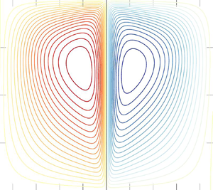
Figure 2. Contours of streamfunction (a,b) and buoyancy (c,d) in a DNS using Dedalus (Burns et al. Reference Burns, Vasil, Oishi, Lecoanet and Brown2020), imposing a  $z$-independent localised heat source around
  $\tilde {x}=0$ which emulates a heated wall, and zero buoyancy and vertical velocity at the top and at the bottom of the domain. Contour values for the streamfunction go from
  $-10$ to
  $+10$ with a spacing of
  $0.5$; blue is clockwise and red is anti-clockwise. Contour values for the buoyancy go from
  $0$ to
  $50$ with a spacing of
  $1.5$. (a,c) Steady state reached at relatively low heating
  $Ra=200$ and
  $\varOmega =1$. (b,d) Instability triggered with increased heating, at
  $Ra=360$ and
  $\varOmega =1$. We do not consider these larger and unstable Rayleigh number solutions further here.
Figure 2(a,c) shows contours of the streamfunction in the steady state, in a DNS with  $L_x = 16$ and
  $H = 7$ (size of the wall, in non-dimensional length units),
  $Ra = 200$,
  $\varOmega =1$ and
  $\sigma /H=7.1 \times 10^{-3}$ (width of the Gaussian, in length units). Two convective cells are created, one flowing clockwise (in blue) and one flowing anti-clockwise (in red). They are symmetric right–left but the up–down symmetry is broken because of buoyancy and gravity. From the bunching of streamlines in the thin layer close to the heated wall, we can infer the existence of a vertical boundary layer in which the flow is accelerated vertically to the top. The right panel in figure 2 shows the instability triggered when the heating is increased further, to
  $Ra = 360$. Here, we focus on the steady solutions, hence the study of this instability is beyond the scope of this work. It is noteworthy that the DNS results in the stable configuration (figure 2a,c) are similar to what is described by Menand, Raw & Woods (Reference Menand, Raw and Woods2003) and Milne & Butler (Reference Milne and Butler2007) for purely compositional plumes in passive porous layers. With a combination of different values of
  $\varOmega$ and
  $Ra$, however, they report different shapes for the buoyant plumes that can be thinner or wider, with an asymmetry between the upper and the lower part. Exported to our configuration, their results point towards a system in which buoyancy transport is dominated by the advection term.
3. Results
We focus primarily on the boundary-layer flow near the wall, supplied by a reservoir of far-field mush. The specific pattern of the far-field return flow may depend more strongly on the far-field boundary conditions – in geophysical applications this might include the geometry of any mush–eutectic phase boundary. But one would expect the leading order characteristics of the near-wall boundary-layer flow to depend primarily on conditions at the heated wall and immediately outside the boundary layer, and be less sensitive to details of the far-field return flow.
Figure 3 presents the global picture of the convective cell. We define four regions, labelled I through IV, based on the flow characteristics and their various scalings close to the wall, which are derived later. In the following subsections, we provide an analytical description of these different types of behaviours observed near the wall.

Figure 3. Regions of different behaviours observed for the flow close to the wall, from left to right: contours of streamfunction in the numerical simulation; along wall profiles of  $b$,
$b$,  $w$ and
  $\partial _z p$; and summary of the scalings predicted by the theory that are derived in § 3.1. DNS run at
  $Ra=200$ and
  $\varOmega =1$.
3.1. Theory
Focusing on the two-dimensional dynamics in the plane  $(x,z)$, we show that (2.16), (2.17) and (2.24), all collapse into a single equation of a single function that will help us to understand the different physical scalings involved in the problem.
From the continuity equation (2.16), we define a streamfunction  $\psi$ so that the horizontal and vertical velocities
  $u$ and
  $w$ are
 \begin{equation} u ={-} \dfrac{\partial \psi}{\partial z} \quad{\mathrm{and}}\quad w = \dfrac{\partial \psi}{\partial x}. \end{equation}
Then, from the horizontal projection of Darcy's law, which involves cross-derivatives of the pressure field and of the streamfunction, we define a potential  $\bar {\varphi }$ so that
  $p$ and
  $\psi$ can be written as
 \begin{equation} p = \dfrac{\partial\bar{\varphi}}{\partial z}\quad {\mathrm{and}}\quad \psi = \dfrac{\partial\bar{\varphi}}{\partial x}. \end{equation}
Using this potential, the horizontal component of Darcy's law is automatically satisfied, and the vertical projection of Darcy's law becomes an equation for  $\bar {\varphi }$ and the buoyancy
  $b$,
$b$,
 \begin{equation} {\nabla}^2 \bar{\varphi} = b. \end{equation}
As a result, all relevant functions of the problem can be expressed using derivatives of the potential  $\bar {\varphi }$, as
 $$\begin{gather} p = \partial_z \bar{\varphi}, \end{gather}$$
 $$\begin{gather}\psi = \partial_x \bar{\varphi}, \end{gather}$$
 $$\begin{gather}u ={-} \partial_x \partial_z \bar{\varphi}, \end{gather}$$
 $$\begin{gather}w = \partial^2_x \bar{\varphi}, \end{gather}$$
 $$\begin{gather}b = {\nabla}^2 \bar{\varphi} = \partial^2_x \bar{\varphi} + \partial^2 _z \bar{\varphi}. \end{gather}$$
 From these results and using the advection–diffusion equation for  $b$ (2.24), we obtain a collapsed equation for
  $\bar {\varphi }$ that is
 \begin{equation} \varOmega [ \partial_t {\nabla}^2 \bar{\varphi} - \partial_x\partial_z\bar{\varphi}\, \partial_x {\nabla}^2 \bar{\varphi} + \partial^2_x\bar{\varphi}\, \partial_z {\nabla}^2 \bar{\varphi}] = {\nabla}^4 \bar{\varphi}. \end{equation}
As  $\varOmega$ is a parameter of order
  $1$, by renormalising the potential
  $\bar {\varphi }$ and the time variable
  $t$ as
 \begin{equation} \bar{\varphi} \rightarrow \frac{1}{\varOmega}\varphi \quad{\mathrm{and}}\quad t \rightarrow \varOmega t,\end{equation}
we can write the equation for  $\varphi$ without explicit dependence on
  $\varOmega$. Hereafter, we use
  $\varphi$ to represent the renormalised quantity according to (3.10a,b). Hence, we have the following equation with three different contributions
 \begin{equation} \partial_t {\nabla}^2 \varphi - \partial_x\partial_z\varphi \partial_x {\nabla}^2 \varphi + \partial^2_x\varphi \partial_z {\nabla}^2 \varphi = {\nabla}^4 \varphi. \end{equation}
This (3.11) represents a balance between temporal evolution of the system  $\partial _t {\nabla }^2 \varphi$, nonlinearities coming from the advection term
  $\partial _x\partial _z\varphi \partial _x {\nabla }^2 \varphi + \partial ^2_x\varphi \partial _z {\nabla }^2 \varphi$ and diffusion of buoyancy
  ${\nabla }^4 \varphi$.
In our study, we will consider steady states for buoyancy and velocity, so the temporal contribution will always be neglected, and relevant balances will involve the nonlinear advection term and the diffusive term. We focus on steady solutions after the initial transient adjustment after warming begins (e.g. figure 2a,c), but note that, at sufficiently large Rayleigh number, the transient dynamics can potentially trigger an instability, as shown in figure 2(b,d). The two nonlinear contributions in (3.11) have the same scaling in terms of numbers of  $x$ and
  $z$ derivatives, due to continuity.
Note that the heat flux boundary condition (2.22) can also be expressed in terms of  $\varphi$ as
 \begin{equation} {-}\partial_x {\nabla}^2 \varphi = Ra \varOmega \quad{\mathrm{at}}\ x=0, \end{equation}
so that the only parameter group in the problem is the modified Rayleigh number  $Ra \varOmega$ which accounts for the effective heat capacity augmented by latent heat release or uptake from the phase change.
The buoyancy is given by the Laplacian of  $\varphi$ and, as such, it involves
  $x$ and
  $z$ derivatives. These derivatives may or may not have the same scalings, which leads to three different idealised cases discussed in the following subsections:
(i) If
 $\partial _x \sim \partial _z$, both derivatives contribute to the buoyancy and the region is isotropic.
(ii) If
$\partial _x \gg \partial _z$, the horizontal variations are more important than the vertical variations, which is characteristic of a vertical boundary layer.(iii) If
$\partial _x \ll \partial _z$, the horizontal variations are less important than the vertical variations, which is characteristic of a horizontal boundary layer.


We now examine the scalings resulting from (3.11) based on these three regimes
3.1.1. Isotropic scaling
We define the following scalings for  $x$,
$x$,  $z$, and
  $\varphi$
 \begin{equation} x,z \rightarrow L\quad {\mathrm{and}}\quad \varphi \rightarrow A, \end{equation}
where  $x$ and
  $z$ have the same scaling due to isotropy.
The scaling of the heat flux boundary condition leads to
 \begin{equation} A \sim Ra \varOmega L^3 \sim L^3. \end{equation}
Since the system is in a steady state, temporal derivatives make no contribution, and the scaling of the remaining terms in the potential equation (3.11) yields
 $$\begin{gather} -\partial_x\partial_z\varphi \partial_x {\nabla}^2 \varphi + \partial^2_x\varphi \partial_z {\nabla}^2 \varphi \sim \frac{A^2}{L^5} \sim Ra^2 \varOmega^2 L, \end{gather}$$
 $$\begin{gather}{\nabla}^4 \varphi \sim \frac{A}{L^4} \sim \frac{Ra \varOmega}{L}, \end{gather}$$
where we eliminate  $A$ using (3.14). This means that the nonlinear terms and the diffusive term have different scalings, in
  $L$ and in
  $1/L$ respectively. Two asymptotic behaviours can therefore be described:
(i) For
$L \ll (Ra\varOmega )^{-1/2}$: the diffusive term dominates the equation and is at least one order of magnitude in $L$ larger than the nonlinear terms. The regime is diffusive, which means that $\boldsymbol {u} \boldsymbol {\cdot } \boldsymbol {\nabla } b \approx 0$, and the buoyancy satisfies a Poisson equation with heat source from the heated wall. From the scaling of $\varphi$ in (3.14), we have $b\sim Ra \varOmega L$ and $w\sim Ra \varOmega L$.(ii) For
$L \gg (Ra\varOmega )^{-1/2}$: the nonlinear terms dominate the equation.


3.1.2. Isotropic stagnation flow scaling
Another explanation for a linear scaling comes from a stagnation point flow model. We illustrate this here for flow near the upper boundary at  $z=H$. A Taylor series expansion of the streamfunction in to second order gives
 \begin{equation} \psi = A x + B z + C x^2 + D x z + E z^2. \end{equation}
Enforcing boundary conditions that  $w=\partial _x \psi =0$ at
  $z=H$ and the symmetry condition
  $u=-\partial _z \psi =0$ at
  $x=0$ yields the following streamfunction:
 \begin{equation} \psi ={-}D x (H-z), \end{equation}
with  $D$ a coefficient to be determined. This suggests a linear scaling in
  $z$ for
  $w$ near to the upper boundary. The coefficient
  $D$ depends on matching to the flow from the incoming isotropic region; this calculation is challenging and not pursued here. A similar analysis yields a corresponding expression
  $\psi \propto xz$ near the lower boundary at
  $z=0$.
3.1.3. Vertical boundary layer
We define the following scalings for  $x$,
$x$,  $z$ and
  $\varphi$:
 \begin{equation} x \rightarrow L_x,\quad z \rightarrow L_z \sim z, \quad{\mathrm{and}}\quad \varphi \rightarrow A, \end{equation}
where  $L_z \sim z$. In this case, the variations along
  $z$ are small compared with the variations along
  $x$ and the scaling length
  $L_x$ is expected to be a function of
  $z$ (cf. similarity solutions of Cheng & Minkowycz Reference Cheng and Minkowycz1977; Guba & Worster Reference Guba and Worster2006).
Temporal derivatives make no contribution in steady state and, given that  $\partial _x \gg \partial _z$, we neglect the
  $z$ derivatives compared with
  $x$ derivatives, so the scaling of the potential equation is given as
 \begin{equation}
{\partial_t {\nabla}^2 \varphi} -
\underbrace{\partial_x\partial_z\varphi \partial_x
(\partial^2_x \varphi {+ \partial^2_z
\varphi}) + \partial^2_x\varphi \partial_z (\partial^2_x
\varphi {+ \partial^2_z
\varphi})}_{\frac{A^2}{L_z L_x^4}} =
\underbrace{\partial^4_x \varphi}_{\frac{A}{L_x^4}}
{+ 2 \partial^2_x \partial^2_z \varphi
+ \partial^4_z \varphi},
\end{equation}
\begin{equation}
{\partial_t {\nabla}^2 \varphi} -
\underbrace{\partial_x\partial_z\varphi \partial_x
(\partial^2_x \varphi {+ \partial^2_z
\varphi}) + \partial^2_x\varphi \partial_z (\partial^2_x
\varphi {+ \partial^2_z
\varphi})}_{\frac{A^2}{L_z L_x^4}} =
\underbrace{\partial^4_x \varphi}_{\frac{A}{L_x^4}}
{+ 2 \partial^2_x \partial^2_z \varphi
+ \partial^4_z \varphi},
\end{equation}
leading to the balance
 \begin{equation} A \sim L_z \sim z. \end{equation}
The same method gives a scaling of the wall heat flux boundary condition (3.12)
 \begin{equation} Ra\varOmega \simeq{-} \underbrace{\partial_x (\partial^2_x \varphi}_{\frac{A}{L_x^3}} {+ \partial^2_z \varphi}), \end{equation}
then
 \begin{equation} L_x \sim \left(\frac{A}{Ra\varOmega}\right) ^{1/3} \propto z^{1/3}. \end{equation}
 From these scalings, we define a characteristic boundary-layer width  $L_x$ as
 \begin{equation} L_x = \frac{h^{2/3} z ^{1/3}}{\varOmega^{1/3}} = z^{1/3} (Ra \varOmega)^{{-}1/3}, \end{equation}
where  $h$ is the dimensionless characteristic length defined from the Rayleigh number and the size of the wall
  $H$ in (2.23). This motivates using a self-similar variable
 \begin{equation} \eta = \frac{x}{L_x} = \frac{x \varOmega^{1/3}}{h^{2/3} z^{1/3}}. \end{equation}
The potential can be written under the form  $\varphi = z f(\eta )$ in terms of a function
  $f$. As we are neglecting the
  $z$ derivatives in the boundary layer, we have
 \begin{equation} w = b = \varOmega^{{-}1} \partial^2 _ x \varphi \quad {\mathrm{and}}\quad p = \varOmega^{{-}1} \partial_z \varphi, \end{equation}
and, since  $\varphi = z f(\eta )$ and
  $L_x$ goes like
  $z^{1/3}$, we obtain the following scalings for
  $w$ and
  $b$:
$b$:
 \begin{equation} w \sim Ra ^{2/3} \varOmega^{{-}1/3} z^{1/3}\quad {\mathrm{and}}\quad b \sim Ra ^{2/3} \varOmega^{{-}1/3} z^{1/3}. \end{equation}
These scalings are analogous to those derived by Cheng & Minkowycz (Reference Cheng and Minkowycz1977) for a self-similar flow at a wall with imposed temperature varying  $T\sim z^{1/3}$, which recovers a constant heat flux. Replacing
  $\varphi = z f(\eta )$ in the collapsed advection–diffusion equation (3.20), we derive a self-similar ordinary differential equation for
  $f$,
$f$,
 \begin{equation} (f'')^2 - 2 f' f''' - 3 f'''' = 0. \end{equation}
The boundary conditions imposed at the wall ( $x=0$) and in the far field (see similar analysis in Cheng & Minkowycz (Reference Cheng and Minkowycz1977) for a boundary layer in a porous medium with wall temperature varying as a power law of distance along the wall, and Guba & Worster (Reference Guba and Worster2006) for a boundary layer next to an isothermal boundary in a solidifying mush layer) are
 \begin{equation} \underbrace{f'''(0) ={-}1}_{\mathrm{flux~at~}x=0},\quad \underbrace{f'(0) = 0}_{u=0\mathrm{~at~the~wall}} \quad\mathrm{and}\quad \underbrace{f''(\eta^*) \rightarrow 0 \quad\mathrm{as}\quad \eta^* \rightarrow \infty }_{\mathrm{constant~}b\mathrm{~in~the~far~field}}. \end{equation}
Note that the final condition of constant buoyancy in the far field is equivalent to zero vertical velocity in the far field outside of the boundary layer. For numerical integration purposes, we set  $f''(\eta ^*) = 0$ at some large value of
  $\eta ^*$ and thereafter check that the solution becomes independent of this choice of
  $\eta ^*$. Although (3.28) is a fourth-order differential equation, only three boundary conditions are required because the physical variables only depend on derivatives of
  $f$ and (3.28) is a third order equation for
  $f'$. We later compute this solution using the Dedalus iterative boundary value problem solver (Burns et al. Reference Burns, Vasil, Oishi, Lecoanet and Brown2020) over
  $256$ Chebyshev nodes, with
  $\eta ^{\star }$ chosen large enough to ensure that the far-field boundary condition is satisfied. Numerical convergence of the solution is obtained after a few iterations.
3.1.4. Horizontal boundary layer
To determine scalings for the horizontal boundary layer near the top boundary, we define the following scalings for  $x$,
$x$,  $z$ and
  $\varphi$
 \begin{equation} x \rightarrow L_x \sim x, \quad z \rightarrow L_z, \quad\mathrm{and}\quad \varphi \rightarrow~ A, \end{equation}
where  $L_x \sim x$ and
  $L_z \ll L_x$ as the variations along
  $x$ are small compared with the variations along
  $z$. The scaling length
  $L_z$ is expected to be a function of
  $x$.
$x$.
Temporal derivatives make no contribution in steady state and, given that  $\partial _x \ll \partial _z$, we neglect the
  $x$ derivatives, so the scaling of the potential equation yields
 \begin{equation} {\partial_t {\nabla}^2 \varphi} - \underbrace{\partial_x\partial_z\varphi \partial_x ({\partial^2_x \varphi +} \partial^2_z \varphi) + \partial^2_x\varphi \partial_z ({\partial^2_x \varphi +} \partial^2_z \varphi)}_{\frac{A^2}{L_z^3 L_x^2}} = {\partial^4_x \varphi + 2 \partial^2_x \partial^2_z \varphi +} \underbrace{\partial^4_z \varphi}_{\frac{A}{L_z^4}}. \end{equation}
Balancing these terms leads to
 \begin{equation} A \sim L_x^2 / L_z \sim x^2 / L_z, \end{equation}
where  $L_z(x)$ has to be determined.
As for the vertical boundary layer, we introduce a similarity variable  $\zeta$ and write the potential
  $\varphi$ in terms of a function
  $g$ as
 \begin{equation} \zeta = \frac{z}{L_z(x)} \quad\mathrm{and}\quad \varphi = \frac{x^2}{L_z(x)} g (\zeta). \end{equation}
 We determine  $L_z (x)$ by assuming that an order-
 $1$ fraction of the buoyant heat flux coming from below towards the top boundary is eventually transported sideways through this upper boundary layer, so that the horizontal spreading flow carries a constant heat flux at leading order. A full solution of the problem will require asymptotic matching of the incoming fluxes. However, to determine the scalings this only needs to be true in an order-of-magnitude sense; the whole buoyant heat flux, corresponding to the heat flux at the entire wall (i.e. sum of the flux
  $-b_x = Ra= 1/h^2$ emitted over the wall of length
  $H$), is going sideways through this top region, meaning
 \begin{equation} \int u b \,\text{d} z \sim \frac{Ra}{h^2}\quad \mathrm{as}\ h \rightarrow 0, \end{equation}
where the integral is over the depth of the horizontal boundary layer. This assumes the heat lost by conduction through the top boundary does not change the order of the magnitude of the heat flux: this approximation should work well for small enough  $x$ sufficiently close to the plume, but may break down sufficiently far downstream where the accumulated heat loss may eventually become substantial. Noting that
  $u=-\partial _x\partial _z\varphi /\varOmega$ and
  $b \approx \partial _z^2 \varphi /\varOmega$ within the boundary layer, computing the left-hand side yields
 \begin{equation} \int u b \,\text{d} z ={-}\frac{1}{\varOmega^2}\frac{x^3}{L_z (x) ^4} \int \left[ g'' (\zeta) \left( 2 g'(\zeta) - \frac{x L'_z (x)}{L_z(x)} \left( \zeta g'' (\zeta) + 2 g' (\zeta) \right)\right) \right] \text{d} \zeta. \end{equation}
If  $L_z$ has power-law dependence on
  $x$, then
  $x L_z'/L_z$ is a constant. Then, the balance of the heat fluxes (3.34) gives
 \begin{equation} L_z (x) = \frac{h^{1/2} x ^{3/4}}{H^{1/4} \varOmega^{1/2}} = x^{3/4} Ra^{{-}1/4} \varOmega^{{-}1/2} , \end{equation}
where, we retain a dimensionless  $H$ in the following calculation to aid interpretation, even though the dimensionless height is
  $1$. Hence, the potential
  $\varphi$ is given as
 \begin{equation} \varphi = \frac{\varOmega^{1/2} H^{1/4} x^{5/4}}{h^{1/2}}g (\zeta) = Ra^{1/4} \varOmega^{1/2} H^{1/4}x^{5/4} g(\zeta). \end{equation}
As we are neglecting the  $x$ derivatives compared with the
  $z$ derivatives,
  $b \simeq \partial _z p$ so that we have
 \begin{equation} w = \varOmega^{{-}1} \partial^2_x \varphi \quad\mathrm{and}\quad b \simeq \partial_z p = \varOmega^{{-}1} \partial_z ^2 \varphi , \end{equation}
which implies that hydrostatic balance holds at leading order in this boundary layer, and the pressure gradient is
 \begin{equation} \partial_z p = \varOmega^{{-}1} \partial_z ^2 \varphi = \frac{\varOmega^{1/2} H^{3/4}}{h^{3/2} x^{1/4}} g'' (\zeta) = Ra^{3/4} \frac{\varOmega^{1/2} H^{3/4}}{x^{1/4}} g''(\zeta). \end{equation}
3.2. Comparison with numerical solutions
Using the above scaling arguments, we can define four different domains for the numerical simulation results presented in figure 3, labelled I, II, III and IV, starting from the bottom of the wall, and correspond to the different scalings derived in the previous subsections. These domains yield contrasting behaviour of the along wall profiles of  $w$,
$w$,  $b$ and
  $\partial _z p$ (see figure 3). The interest in these three quantities is motivated by the relation
  $b = {\nabla }^2 \varphi = w + \partial _z p$, showing that the buoyancy, the vertical velocity, and the vertical pressure gradient, are linearly related.
These four regions have different scalings, that can be explained as follows.
a. Region I Tip behaviour, in a small regularisation region. All quantities are small and the region is isotropic. Diffusive terms dominate and the buoyancy approximately satisfies a Laplace equation for diffusive heat transfer in steady state. Because this region is isotropic, we expect the variation along the length of the wall to satisfy
$w\sim z$ and $b\sim z$ as discussed in § 3.1.1.b. Region II Rising plume region, described by a vertical boundary layer in which horizontal spatial derivatives dominate. The vertical Darcy flow is driven by buoyancy forces with pressure gradients negligible, yielding
$b \simeq w$. Due to the vertical boundary layer, $z^{1/3}$ scalings are expected as discussed in § 3.1.3.c. Region III Connection region, between II and IV, where
$b$, $w$ and $\partial _z p$ are of the same order of magnitude. The region is isotropic and the nonlinear terms dominate the collapsed equation. The incoming plume flow from below carries most of the buoyancy flux, which is advected through this region and the additional heating at the wall does not change the buoyancy flux substantially, remaining of the same order of magnitude throughout this region. An empirical power law of $w \propto (H-z)^{1/3}$ and $b \propto (H-z)^{-1/3}$ scalings are discussed in § 3.2.3.d. Region IV Top corner region, with the scaling of a top boundary layer, bringing the heat flux sideways into the horizontal boundary layer. Again, this region is diffusive and we expect the linear scalings, similar to those derived in § 3.1.1 except using the distance to
$(0,H)$. Region IV forms part of the turnaround region, where the initially vertical flow adjusts into horizontal flow towards a region that grows with $x$ with a horizontal boundary layer as in § 3.1.4 and its scalings for the pressure gradient. Region IV can be decomposed into two distinct regions, with a corner region close to the top of the wall, which develops into an adjacent region as a horizontal top boundary layer. We hypothesise that the pressure gradient from the horizontal boundary layer is imprinted on the corner region, leading to a unique pressure scaling for region IV.


In figure 4, we present  $\log$–
 $\log$ plots of the vertical velocity and of the buoyancy in which the different scalings predicted analytically in the previous subsections are tested. Figure 4(a,b) shows
  $\log$–
 $\log$ plots of the vertical velocity along the wall, with distance from the bottom and distance from the top, respectively. We first observe a linear scaling
  $w\propto z$ in region I, behaviour potentially consistent with two
  $1/3$ scalings
  $w\propto z^{1/3}$ and
  $w\propto (H-z)^{1/3}$ in region II and III, and a linear scaling
  $w\propto (H-z)$ in region IV. Figure 4(c,d) shows
  $\log$–
 $\log$ plots of the buoyancy varying with distance along the wall, starting from the bottom and starting from the top, respectively. Similarly to the vertical velocity, we first observe a linear scaling
  $w\propto z$ in region I, a
  $1/3$ scaling
  $w\propto z^{1/3}$ in region II and a
  $-1/3$ scaling
  $w\propto (H-z)^{-1/3}$ in region III and a linear scaling
  $w\propto (H-z)$ in region IV. As discussed above, scalings for regions I, II, and IV, are consistent with the theoretical expectations. Region III, however, shows interesting empirically suggested scalings for which we do not yet have an asymptotic explanation. We now compare our scaling predictions with the numerics in more detail.

Figure 4. Scalings inferred from the profiles obtained in the DNS along the wall (at  $x=0$). Blue lines show (a) vertical velocity varying with distance from the bottom; (b) vertical velocity varying with distance from the top; (c) buoyancy varying with distance from the bottom; and (d) buoyancy varying with distance from the top. Red lines indicate slope of linear scalings, green lines for
  $+1/3$ power law and cyan lines for
  $-1/3$ power law. The different regions are indicated by the labels I, II, III and IV.
3.2.1. Region I
Close to the bottom tip, the vertical velocity, the buoyancy and the pressure gradient are small (figure 3). All terms contribute to the equations as the region is isotropic. The scalings described in § 3.1.1 show that, because the length scale is small, this region is diffusive and has a linear scaling for  $b$ and
  $w$ with
  $z$, that is observed in figure 4(a,c). This region breaks down when the isotropic scale
  $L_x \sim z$ becomes comparable to the width
  $L_x \sim h^{2/3} z^{1/3}$ of a potential rising plume, i.e. when
  $z$ is of order
  $h$.
$h$.
3.2.2. Region II
In region II, the flow acts like a rising buoyant plume described by the vertical boundary layer from § 3.1.3. The flow structure is similar to the analysis performed by Guba & Worster (Reference Guba and Worster2006) but with some differences in the power-law scalings in the similarity solution: where Guba & Worster (Reference Guba and Worster2006) derived a self-similar variable in  $z^{-1/2}$ and velocity and buoyancy scalings in
  $z^{1/2}$ for an isothermal wall, we here derive solutions for a constant flux wall with a self-similar variable in
  $z^{-1/3}$ yielding velocity and buoyancy scalings in
  $z^{1/3}$. Note that these scales match the Cheng & Minkowycz (Reference Cheng and Minkowycz1977) solution with a similarity power scaling of
  $1/3$. By equating the length scales
  $L_x$ between region I and region II, we see that the lateral extent of this region at the bottom, connecting to region I, is initially of order
  $h$, and thereafter increases proportional to
  $h^{2/3} z^{1/3}$. From (3.27a,b), our theory predicts a scaling in
  $z^{1/3}$ for
  $w$ and
  $b$ with the numerical solutions appearing to approach this scaling for intermediate
  $z$ in the
  $\log$–
 $\log$ plot in figure 4(a,c). In figure 5, we present horizontal slices of the vertical velocity (a,b) and of the buoyancy (c,d) at different depths in region II (plain lines), rescaled in the horizontal variable by
  $z^{1/3}$ as well as in amplitude. We observe a good collapse at
  $x=0$, close to the wall. The superimposed dashed line is the self-similar solution of (3.28) and (3.29a–c). Note that the scale separation between the start
  $z=O(h)$ and end
  $z=O(1)$ of this region is quite modest for the given Rayleigh number
  $Ra=200$, and there is only around a decade for the power-law scaling to adjust. Whilst the scale separation would increase for a steady laminar flow at higher
  $Ra$, our simulations (figure 2b) revealed that instability and unsteady flow develops at larger
  $Ra$.
$Ra$.

Figure 5. Horizontal slices of vertical velocity  $w$ and buoyancy
  $b$ at different depths in region II (at
  $z=0.34$ (blue),
  $z=0.39$ (orange),
  $z=0.44$ (red) and
  $z=0.49$ (yellow)), with (a)
  $w$ vs
  $x$ for different
  $z$; (b) collapsed
  $w$ vs collapsed
  $x$; (c)
  $b$ vs
  $x$ for different
  $z$; and (d) collapsed
  $b$ vs collapsed
  $x$. The self-similar solution to (3.28)–(3.29a–c) is superimposed on the rescaled profiles in (b,d) (dashed line).
The computed solutions show a good agreement with the data. The profiles diverge from the similarity solution in the far field, due to the influence of the return flow and its impact on the background buoyancy field that is not included in the boundary-layer model. Nevertheless, the similarity variables yield a good collapse of the shape of decay of the velocity and buoyancy profiles away from the heat source, their characteristic boundary-layer width and capture their leading-order quantitative magnitude. We note that the peak in  $w$ measured from the DNS is not as large as predicted by the similarity solution: this might be due to the neglect of the pressure gradient term in the leading-order balance for the similarity solution, which acts to slightly decelerate the flow in the full numerical solution.
3.2.3. Region III
Region III is an isotropic region connecting regions II and IV. Figure 3(b) shows how the force balance in this connection region behaves. We recall that  $b = w + \partial _z p$ from Darcy's law (2.16). In region II, as seen before, the vertical boundary layer model leads to
  $w \simeq b$ and
  $\partial _z p$ is negligible, whereas in region IV,
  $b \simeq \partial _z p$ and
  $w$ has a small contribution (see figure 3b). The only way this configuration can occur is to have an isotropic transition region in between, in which
  $w$ and
  $\partial _z p$ have the same order of magnitude, with
  $w$ decreasing while
  $\partial _z p$ increases. This behaviour is observed in domain III in figure 3(b).
From the  $\log$–
 $\log$ plots in figure 4(b,d), we infer two empirical scalings: a
  $(z-H)^{1/3}$ scaling for
  $w$, and a
  $(z-H)^{-1/3}$ scaling for
  $b$. Figure 6 presents horizontal slices of vertical velocity (a,c) and buoyancy (b,d) rescaled by
  $1/3$ and
  $-1/3$ power laws, showing a good collapse close to the wall. A deviation in the far field, due to the return flow outside of the boundary layer, is observed. The collapse is better for
  $w$ than for
  $b$, pointing towards a transition between a vertical boundary layer in which
  $w$ is set and a fully isotropic region dominated by fluxes. This collapse, however, is curious as it does not correspond to the boundary layer described in the previous sections, and still awaits a theoretical explanation which we reserve for future work. Note that this scaling implies that the product
  $wb$ is approximately constant, which means that the heat flux advected through this region III also remains approximately constant.

Figure 6. Horizontal slices of vertical velocity  $w$ and buoyancy
  $b$ at different depths in region III (at
  $z=0.65$ (blue),
  $z=0.70$ (orange),
  $z=0.75$ (red) and
  $z=0.80$ (yellow)), with (a)
  $w$ vs
  $x$ for different
  $z$; (b) collapsed
  $w$ vs collapsed
  $x$; (c)
  $b$ vs
  $x$ for different
  $z$; and (d) collapsed
  $b$ vs collapsed
  $x$.
$x$.
3.2.4. Region IV
In the top corner region IV, both the scalings of  $b$ and
  $w$, linear with
  $H-z$ (see figure 4), are consistent with a stagnation point flow. The velocity profile decelerates to satisfy the non-normal flow boundary condition at the top, and we observe the dominance of diffusive transfers of buoyancy as the velocity decays to zero in the corner.
We also note that the pressure gradient is consistent with the imprint of scalings in the neighbouring horizontal boundary layer in which the flow spreads horizontally. In this region, the pressure gradient reaches a maximum and balances the buoyancy force at leading order. According to (3.39), the peak in the vertical profile of the pressure gradient should increase and move upwards as we increase the Rayleigh number. Figure 7 shows results from DNS at various Rayleigh numbers, with this increasing peak. For each of these profiles, we measure the amplitude of the peak  $\max (\partial _z p)$ and its location
  $z_m$ from the top of the wall. Figure 8 presents these data in
  $\log$–
 $\log$ plots. For the amplitude of the peak (figure 8a) we have a
  $Ra^{3/4}$ scaling (or
  $h^{-3/2}$) consistent with the theory developed in § 3.1.4. For the location
  $z_m$ (figure 8b), we have a
  $Ra^{-1/2}$ scaling (or
  $h$) for
  $H-z_m$, which is linked to the cross-over length scale derived in § 3.1.1 where both the nonlinear advective and diffusive terms become of similar magnitude. Note that the testing of these scalings in figure 8 is limited in the range of accessible Rayleigh numbers: at low
  $Ra$, the flow stops convecting and there are no boundary layers in which our model would apply; conversely, at high
  $Ra$ (we have not characterised the precise instability threshold, but our brief numerical investigation suggests above 300–350), the near-crack instability is triggered (see figure 2) and the theoretical derivation does not hold anymore.

Figure 7. Along wall profiles of the vertical pressure gradient for different Rayleigh numbers (corresponding to different heating prefactors  $Q_0$).

Figure 8. Scaling laws for along wall pressure with Rayleigh number in  $\log$–
 $\log$ plots. The shades of blue correspond to the Rayleigh numbers indicated in figure 7. (a) Amplitude of the peak of pressure gradient, with a
  $Ra^{3/4}$ law. (b) Location of the maximum of the pressure gradient, as a distance from the top boundary, with a
  $Ra^{-1/2}$ law.
We present, in figure 9, vertical slices of the horizontal velocity  $u$ and of the buoyancy
  $b$ unscaled (a,c) and rescaled by the scalings predicted by the theory (b,d). The self-similar scalings works relatively well in a thin boundary layer close to the top boundary
  $z=H$ but breaks further below. It is likely that there is some more complex behaviour going on with the spreading horizontal boundary layer fed by the rising plume, with another diffusive boundary layer nested within this due to the cooling boundary condition that
  $b=0$ at the top of the domain.

Figure 9. Vertical slices of horizontal velocity  $u$ and buoyancy
  $b$ at different locations
  $x$ in region IV (measured from the crack: at
  $x=0.24$ (blue),
  $x=0.36$ (orange),
  $x=0.48$ (red) and
  $x=0.60$ (yellow)), with (a)
  $u$ vs
  $(H-z)$ for different
  $x$; (b) collapsed
  $u$ vs collapsed
  $(H-z)$; (c)
  $b$ vs
  $(H-z)$ for different
  $x$; and (d) collapsed
  $b$ vs collapsed
  $(H-z)$.
3.3. Prediction of the solid dissolution rate
We now discuss the phase change behaviour close to the wall. We have previously shown that the flow transports solute which can drive either local dissolution of the ice matrix, or freezing, which modify the solid fraction.
The advection–diffusion equation for  $b$ and the solute and heat equations give an equation for the evolution of the solid fraction
  $\phi$, or melting rate, depending on the potential
  $\varphi$. At first order, the solid fraction can be written
  $\phi = \phi _0 + \hat {\phi }$, where
  $\phi _0$ is the initial value and
  $\hat {\phi }$ the perturbation away from the steady state. Recalling that the near-eutectic approximation leads to
  $b(1-\phi )\approx b (1-\phi _0)$, then (2.15) yields an equation for
  $\partial \phi /\partial t$ in terms of
  $b$. Substituting for
  $(1-\phi _0) \partial b/\partial t+\boldsymbol {u}\boldsymbol {\cdot } \boldsymbol {\nabla } b$ using (2.24) and noting that
  $b = \nabla ^2 \varphi /\varOmega$, in dimensionless form this yields
 \begin{equation} \dfrac{\partial \hat{\phi}}{\partial t} ={-}\frac{1}{\mathscr{C} Ra} \left[ (1-\phi_0)\frac{\partial b}{\partial t} + (\boldsymbol{u} \boldsymbol{\cdot} \boldsymbol{\nabla}) b\right] ={-}\frac{1}{\mathscr{C} Ra \varOmega} {\nabla}^4 \varphi. \end{equation}
As we are looking at quasi-steady tendencies on the porosity, we do not include the time-dependent feedback on  $b$ and therefore set
  $\partial b/\partial t=0$. Therefore, the intermediate expression in (3.40) indicates the role of the advection of salinity anomalies, and hence buoyancy anomalies, in controlling the phase change. There is a tendency for reduction in solid fraction by local dissolution when
  $\boldsymbol {u} \boldsymbol {\cdot } \boldsymbol {\nabla } b >0$, which corresponds to an advection of saline fluid with low buoyancy into a fresher region with higher buoyancy. As described by Worster (Reference Worster1997) and Butler (Reference Butler2011), this phenomenon arises because solute advects more rapidly than heat in a passive porous layer, so the salinity front runs ahead of the thermal front and ice melts in order to reduce the salinity and restore a thermodynamic equilibrium. In this model, we assume that the system reaches a steady state for the flow, the buoyancy, and the temperature. We have neglected the feedback from porosity variation on the flow (
 $\varPi$ is a constant and is equal to
  $\varPi _0$) which allows for such a quasi-steady state with slowly evolving porosity and non-zero
  $\partial _t \phi$. Hence, the neglect of transient porosity changes should be reasonable at early times, but will eventually break down at longer time as the accumulated porosity change becomes large. Due to the different behaviours in the aforementioned regions, there are presumably two different time scales according to which the porosity evolves. In region II, accounting for the narrow vertical boundary-layer thickness, we get a melting rate
  $\partial _t \hat {\phi } \sim - Ra^{1/3} \varOmega ^{1/3} / \mathscr {C}$. In the corner region IV, using that
  $b\sim \partial _z p \sim Ra^{3/4}$, and
  $\nabla ^2 b \sim b/h^2$, we obtain a melting rate
  $\partial _t \hat {\phi } \sim Ra^{3/4} \varOmega ^{1/2} / \mathscr {C}$. This suggests a larger freezing rate in the top region, in agreement with our observations.
The instantaneous melting rate predicted by (3.40) using the DNS is presented in figure 10, in which areas with decreasing solid fraction are shown in red. This indicates instantaneous melt rate deviation away from steady state. Negative value for  $\nabla ^4 \varphi \propto - \partial _t \hat {\phi }$ means that the solid fraction is increasing, corresponding to ice solidifying. A strong and localised region of solidification is identified at the top of the crack, corresponding to region IV, with a vertical extent of order
  $h$, which confirms the importance of the top region in the melting problem. Such freezing is caused by upward advection of solute and a net convergence of the solute flux in the diffusive boundary layer in the upper corner region. Note that this region is direct analogue to the region of localised freezing identified and discussed in Guba & Worster (Reference Guba and Worster2006). An additional region of melting can be seen close to the wall, next to the heated melting region which corresponds to the tendency for advection by the rising plume to enrich the initial background of solute and cause melting. Because the solution predicts flow through regions of instantaneous freezing, it would only be valid for a system that initially has non-zero porosity and cannot be applied directly to an initial condition with pure eutectic solid. The melting occurring close to the crack is a slower process than the freezing, as
  $\partial _t \hat {\phi }$ varies over more than an order of magnitude between the freezing and the melting region at the crack, and even more if we look at the top region. On longer time scales, it is likely that this behaviour would be suppressed with a feedback of the porosity on the flow, as a solid fraction equal to
  $1$ would prevent the liquid from flowing. The relevant scalings, however, are still a good approximation of what is happening for a system starting with non-zero porosity at early times. Understanding the impact on porosity-dependent feedbacks on permeability, and evolution from an initially solid state represent interesting challenges for future work.

Figure 10. Dissolution rate, or solid fraction change predicted by the steady state flow and buoyancy fields, from the numerical simulation (red shows melting). The white dotted lines show the locations  $\pm \sigma$ used for the Gaussian heat flux, at
  $Ra=200$ and
  $\varOmega =1$. Note that the scaling of (3.40) and the prediction of melt rate break down in our simulations over a length scale comparable to the white dashed lines due to the use of an added volumetric heat source rather than a boundary flux.
4. Conclusions and discussion
In this study, we developed a simple model of a buoyant plume generated by a heated wall with constant heat flux in an ideal mushy zone using a near-eutectic limit. We identified four different regions created along the wall through the heating process, and we show that the relevant part that dominates the melting is located near the surface over a short depth  $h \propto Ra^{-1/2}$ (to within a multiplicative factor depending on the modified heat capacity
  $\varOmega$). The proposed mechanism is robust, with local scalings holding for a wide range of Rayleigh number, and the different scalings observed in DNS agree well with the theory that uses asymptotics and self-similar solutions. From top to bottom these demonstrate an isotropic diffusive region I with linear scalings for buoyancy and velocity with height develops into a buoyant self-similar rising plume region II which scalings are given by a vertical boundary-layer theory. Region II is connected to a top region IV through an isotropic region III. Region IV has a vertical velocity scaling consistent with a stagnation point flow, and the pressure gradient scaling imposed by an adjacent horizontal boundary layer that develops sidewards with approximate hydrostatic balance in the vertical.
Some empirically diagnosed scalings remain to be explained, however. In region III there are two different scalings for the buoyancy and the vertical velocity that are not theoretically explained. In this region, it is very likely that the vertical velocity matches with region II whereas the buoyancy and the pressure fields match with region IV, and that the total heat flux is conserved, but we have no supporting mathematical theory. No analytical result for region I, at the bottom of the crack, has been properly derived. The top region IV could be better understood by defining regions IV and V: one being the top corner, the other one being the horizontal boundary layer that extends near the surface in the  $x$ direction. Different scalings can then be tested in region V accordingly to the horizontal boundary-layer theory from § 3.1.4.
The vertical extension of the top region can be estimated through the Rayleigh number, as  $Ra= (H / h) ^{2}$. From the previous derivation, noting that the relevant temperature scale in this problem is
  $\Delta T = FH/C_p \kappa$, the Rayleigh number can be expressed into a porous medium Rayleigh number as
 \begin{equation} Ra = \frac{g\alpha \Delta T \varPi_0 H}{\kappa \nu}. \end{equation}
In the case of icy satellites (e.g. Enceladus or Europa), we treat the planetary ice shell as having sea ice material properties and lower gravity on account of planetary size. Hence, due to the range of values for the different parameters involved in the problem if we estimate orders of magnitude for Enceladus such as  $g=10^{-1}\ \mathrm {m}\ \mathrm {s}^{-2}$,
  $\alpha = 10^{-2}\ \mathrm {K}^{{-1}}$,
  $\kappa = 10^{-7}\ \mathrm {m}^2\ \mathrm {s}^{{-1}}$,
  $\nu = 10^{-6}\ \mathrm {m}^2\ \mathrm {s}^{{-1}}$,
  $\Delta T \sim 10^2\ \mathrm {K}$,
  $\varPi _0 \sim 10^{-14}\ \mathrm {m}^{2}$ (lower value than used for terrestrial sea ice (e.g.
  $\varPi _0 = 10^{-10} \text {--}10^{-12} \ \mathrm {m}^{2}$ in Polashenski et al. Reference Polashenski, Golden, Perovich, Skyllingstad, Arnsten, Stwertka and Wright2017) since it is a colder and less open ice) and
  $H \sim 10^3\text {--}10^4\ \mathrm {m}$, we obtain a relatively small Rayleigh number
  $Ra$, approximately
  $10$–
$10$– $100$. A simple estimate indicates that the top region, in which large vertical pressure gradients are predicted, has a small extension of order
  $O(h) \ll H$ and that the high melting region is therefore located near the surface.
Increasing the Rayleigh number further triggers an instability near the wall (see figure 2) and the present model of steady flow is not valid anymore. Starting from the linear steady state, such an instability could occur with an intense and short lived forcing generating large heat fluxes, which might be enough to create strong intermittent melting spots close to the heated wall. This unstable regime is very sensitive to slight changes in Rayleigh number (see figure 2) and its threshold remains to be determined, which will be the focus of future studies.
The geophysical setting of heated cracks in a planetary ice shell contains several complexities not included in the present model. A more accurate description of the problem could be derived, relaxing the constant permeability assumption. The flow would then feel a feedback from the melting of the mush and the phase change itself, as the permeability would be a function of the solid fraction. The geometry of the mushy region generated by melting may also introduce added complexity, as there may be an interface between the mushy region and the pure ice region, that can evolve through time as the mush is growing rather than the rectangular cavity considered here. Provided the mushy region extends beyond the extent of the boundary layers identified here, the present analysis should provides insights relevant to the more complex setting for the far-field flow.
Acknowledgements
We dedicate this work to the memory of C. Doering. He was present at Walsh Cottage when this work was instigated. We enjoyed many conversations with him about convection and topics related to this work. He will be sorely missed.
Funding
The authors are grateful for the NSF OCE-1829864 support during the 2019 GFD Summer School at WHOI. S.B. also thanks IDEX Lyon for additional travel funds.
Declaration of interests
The authors report no conflict of interest.


