2.1. Mathematical statement and 3DA equations

The system is isothermal and consists of an infinite liquid column or jet of an incompressible Newtonian fluid of constant density $\rho$ and constant viscosity $\mu$ of unperturbed radius $R$ that is surrounded by a dynamically passive ambient gas that simply exerts a constant pressure on the jet which is taken here to be the pressure datum. 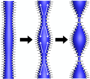The surface of the jet – the liquid–gas (L–G) interface – is covered with a monolayer of an insoluble surfactant and the surface tension of the L–G interface when it is devoid of surfactant is given by $\sigma _p$ (figure 1). The dynamics is taken to be axisymmetric about the centreline of the initially cylindrical column. Thus, it proves convenient to use a cylindrical coordinate system $(\tilde {r}, \theta , \tilde {z})$ with its origin located along the centreline of the initially cylindrical column and where $\tilde {z}$ is the axial coordinate measured along the column's axis, $\tilde {r}$ is the radial coordinate measured from that axis and $\theta$ is the usual angle measured around the symmetry axis $\tilde {r} = 0$. When subjected to axisymmetric shape perturbations of infinitesimal amplitude whose wavelength in the axial direction is given by $\tilde {\lambda }$, a quiescent cylindrical column of liquid undergoes capillary or Rayleigh–Plateau instability if $\tilde {\lambda }>2{\rm \pi} R$ or $\tilde {k} R < 1$ where $\tilde {k} = 2{\rm \pi} / \tilde {\lambda }$ is the wavenumber (Plateau Reference Plateau1873; Rayleigh Reference Rayleigh1878; Michael Reference Michael1981). In this paper, the capillary pinching of a surfactant-covered, quiescent liquid column is initiated by subjecting its surface $\tilde {S}(\tilde {t})$, where $\tilde {t}$ is time, at time $\tilde {t} = 0$ to a shape perturbation of sufficiently long wavelength but of arbitrary amplitude so that the column's profile is given by

(2.1)\begin{equation} \frac{\tilde{r}(\tilde{z}, \tilde{t} = 0)}{R} = \sqrt {1 - \frac {\epsilon ^2}{2}} + \epsilon \cos \tilde{k} \tilde{z} . \end{equation}

When the disturbance amplitude is small, $\epsilon \ll 1$, (2.1) simplifies to $\tilde {r} (\tilde {z}, 0)/R = 1 + \epsilon \cos \tilde {k} \tilde {z}$. Two types of initial conditions are considered for surfactant concentration. In most cases, the jet is taken at $\tilde {t} = 0$ to be coated uniformly with surfactant at concentration $\tilde {\varGamma }_0$. In some cases, the concentration at the surface of a uniformly coated perfectly cylindrical column is perturbed in an analogous manner as its shape (see below).

Figure 1. Definition sketch. (a) A liquid jet the surface $\tilde {S}(\tilde {t})$ of which is covered by a monolayer of an insoluble surfactant. To initiate capillary thinning and pinch-off, the surface of a perfectly cylindrical column of radius $R$ is subjected at time $\tilde {t} = 0$ to an axially periodic sinusoidal perturbation of wavelength $\tilde {\lambda } = 2{\rm \pi} / \tilde {k}$. (b) Domain of interest for 3DA or 2-D analysis. Here, the interface is parametrized by arc length $\tilde {s}$. (c) The 1-D domain. In both the 2-D and 1-D analyses, the axial extent of the domain is $0\le z \le \tilde {\lambda }/2 = {\rm \pi}/\tilde {k}$.

The dynamics of the thinning and breakup of the jet is analysed by solving the transient free boundary problem consisting of the continuity and Navier–Stokes equations for fluid velocity $\tilde {\boldsymbol {v}}$ and pressure $\tilde {p}$ within the jet $\tilde {V}(\tilde {t})$ and the convection–diffusion equation for surfactant concentration $\tilde {\varGamma }$ on $\tilde {S}(\tilde {t})$:

(2.2)\begin{gather} \tilde{\boldsymbol{\nabla}} \boldsymbol{\cdot} \tilde{\boldsymbol{v}}=0 \quad \text{in}\ \tilde{V}(\tilde{t}), \end{gather}

(2.3)\begin{gather} \rho \left(\frac{\partial \tilde{\boldsymbol{v}}}{\partial \tilde{t}}+(\tilde{\boldsymbol{v}} \boldsymbol{\cdot} \tilde{\boldsymbol{\nabla}}) \tilde{\boldsymbol{v}} \right) = \tilde{\boldsymbol{\nabla}} \boldsymbol{\cdot} \tilde{\boldsymbol{\mathsf{T}} \quad \text{in}\ \tilde{V}(\tilde{t}),} \end{gather}

(2.4)\begin{gather} \frac{\partial \tilde{\varGamma}}{\partial \tilde{t}} +\tilde{\boldsymbol{\nabla}}_s \boldsymbol{\cdot} \left(\tilde{\varGamma} \tilde{\boldsymbol{v}} \right) = D_s\tilde{\boldsymbol{\nabla}}_s^2\tilde{\varGamma} \quad {\text{on }} \tilde{S}(\tilde{t}). \end{gather}

In (2.3), $\tilde {\boldsymbol{\mathsf{T}} } = -\tilde {p} \boldsymbol{\mathsf{I}} + \mu [ \tilde {\boldsymbol {\nabla }} \tilde {\boldsymbol {v}}+(\tilde {\boldsymbol {\nabla }} \tilde {\boldsymbol {v}})^T]$ is the total stress tensor for a Newtonian fluid and $\boldsymbol{\mathsf{I}} $ is the identity tensor. In (2.4), $D_s$ is the surfactant diffusivity, $\tilde {\boldsymbol {\nabla }}_s \equiv \boldsymbol{\mathsf{I}} ^s \boldsymbol {\cdot } \tilde {\boldsymbol {\nabla }}$ is the surface gradient operator and $\boldsymbol{\mathsf{I}} ^s \equiv \boldsymbol{\mathsf{I}} -\boldsymbol {n}\boldsymbol {n}$ is the surface identity tensor with $\boldsymbol {n}$ denoting the outward pointing unit normal to $\tilde {S}(\tilde {t})$.

As (2.2) and (2.3) are balances of mass and momentum conservation in the bulk $\tilde {V}(\tilde {t})$, the corresponding principles of mass and momentum conservation at the L–G interface $\tilde {S}(\tilde {t})$ are the kinematic and traction boundary conditions (Scriven Reference Scriven1960; Aris Reference Aris2012). In the absence of bulk flow or mass transfer across the interface, the kinematic boundary condition is given by

(2.5)\begin{equation} \boldsymbol{n} \boldsymbol{\cdot} \left( \tilde{\boldsymbol{v}} - \tilde{\boldsymbol{v}}_s \right) = 0, \end{equation}

where $\tilde {\boldsymbol {v}}_s$ is the velocity of points on the interface. If the surface of the jet is described as a compressible, two-dimensional Newtonian fluid, surface rheological effects that arise over and beyond the ordinary capillary and Marangoni stress effects obey the Boussinesq–Scriven constitutive equation (Scriven Reference Scriven1960). Then the traction or the stress-balance boundary condition at the free surface is given by

(2.6)\begin{align} \boldsymbol{n} \boldsymbol{\cdot} \tilde{\boldsymbol{\mathsf{T}} } &= 2\tilde{\mathcal{H}}\tilde{\sigma}\boldsymbol{n} + \tilde{\boldsymbol{\nabla}}_s\tilde{\sigma} + 2\tilde{\mathcal{H}} \left(\mu_d - \mu_s \right)\left(\tilde{\boldsymbol{\nabla}}_s \boldsymbol{\cdot} \tilde{\boldsymbol{v}}\right)\boldsymbol{n}\nonumber\\ &\quad + \tilde{\boldsymbol{\nabla}}_s\left[\left(\mu_d-\mu_s\right)\left(\tilde{\boldsymbol{\nabla}}_s \boldsymbol{\cdot} \tilde{\boldsymbol{v}}\right)\right] +\tilde{\boldsymbol{\nabla}}_s \boldsymbol{\cdot} \left[\mu_s\left(\tilde{\boldsymbol{\nabla}}_s\tilde{\boldsymbol{v}} \boldsymbol{\cdot} \boldsymbol{\mathsf{I}} ^s + \boldsymbol{\mathsf{I}} ^s \boldsymbol{\cdot} \left(\tilde{\boldsymbol{\nabla}}_s\tilde{\boldsymbol{v}} \right)^T\right)\right]. \end{align}

Here, $2\tilde {\mathcal {H}} \equiv -\tilde {\boldsymbol {\nabla }} \boldsymbol {\cdot } \boldsymbol {n}$ is twice mean curvature of the free surface. The first two terms on the right-hand side of (2.6) correspond to the capillary pressure and the Marangoni stress due to surface tension gradients. The remaining terms account for surface rheological effects. Surface tension $\tilde {\sigma } = \tilde {\sigma } (\tilde {\varGamma })$ as well as the surface shear $\mu _s = \mu _s (\tilde {\varGamma })$ and the surface dilatational $\mu _d = \mu _d (\tilde {\varGamma })$ viscosities are all functions of surfactant concentration $\tilde {\varGamma }$ (see below).

Here, surface tension $\tilde {\sigma }$ is related to surfactant concentration $\tilde {\varGamma }$ via the Szyszkowski equation of state (Liao et al. Reference Liao, Franses and Basaran2006)

(2.7)\begin{equation} \tilde{\sigma} = \sigma_p + \tilde{\varGamma}_m R_g T \ln \left(1-\frac{\tilde{\varGamma}}{\tilde{\varGamma}_m} \right) , \end{equation}

where $\tilde {\varGamma }_m$ is the maximum packing density of surfactant, $R_g$ is the gas constant and $T$ is the absolute temperature. It will be shown below that the particular equation of state adopted to relate surface tension to surfactant concentration is immaterial as the pinch-off singularity is approached.

Since surface rheological effects arise when surfactants deform against themselves at interfaces, it accords with intuition that surface viscosities are functions of $\tilde {\varGamma }$. Although it is not known whether the functional form of $\mu _d(\tilde {\varGamma })$ is identical to that of $\mu _s(\tilde {\varGamma })$, the simplifying assumption is adopted in this paper that $\mu _d$ varies with $\tilde {\varGamma }$ in the same way as $\mu _s$. Throughout the body of the paper, following recent works in the literature (Ponce-Torres et al. Reference Ponce-Torres, Montanero, Herrada, Vega and Vega2017), the surface viscosities are taken to vary linearly with $\tilde {\varGamma }$ with respect to a reference state

(2.8a,b)\begin{equation} \mu_s=\mu_{sr} \tilde{\varGamma}/\tilde{\varGamma}_r, \quad \mu_d=\mu_{dr} \tilde{\varGamma}/\tilde{\varGamma}_r, \end{equation}

where $\mu _{sr}$ and $\mu _{dr}$ are the reference surface viscosities at the reference surfactant concentration $\tilde {\varGamma }_r$. As shown in appendix A, some of the key results presented in this paper can be readily generalized so that they are independent of the constitutive equation used to relate surface viscosities to surfactant concentration.

Because the dynamics is axisymmetric about the $\tilde {z}$-axis, the shear stress and the radial velocity have to vanish at $\tilde {r} = 0$, viz. $\boldsymbol {e}_r \boldsymbol {\cdot } \tilde {\boldsymbol{\mathsf{T}}} \boldsymbol {\cdot } \boldsymbol {e}_z = 0$ and $\tilde {u} \equiv \tilde {\boldsymbol {v}} \boldsymbol {\cdot } \boldsymbol {e}_r = 0$ where $\boldsymbol {e}_r$ and $\boldsymbol {e}_z$ stand for the unit vectors in the radial and axial directions. On account of the periodicity of the imposed initial perturbation of the jet's surface, the problem only needs to be solved over an axial distance equal to one half of the wavelength of the imposed perturbation. Thus, along the two symmetry planes located at $\tilde {z}=0$ and $\tilde {z}={\rm \pi} /\tilde {k} = \tilde {\lambda }/2$, both the shear stress and the axial velocity must vanish, viz. $\boldsymbol {e}_z \boldsymbol {\cdot } \tilde {\boldsymbol{\mathsf{T}}} \boldsymbol {\cdot } \boldsymbol {e}_r = 0$ and $\tilde {v} \equiv \tilde {\boldsymbol {v}} \boldsymbol {\cdot } \boldsymbol {e}_z = 0$. Also because of symmetry, surfactant concentration must obey $\boldsymbol {e}_z \boldsymbol {\cdot } \tilde {\boldsymbol {\nabla }}_s\tilde {\varGamma } = 0$ at $\tilde {z}=0$ and $\tilde {z}={\rm \pi} /\tilde {k}$.

2.2. The 1-D slender-jet equations

Since the jet radius is small relative to the length of the jet, a set of 1-D slender-jet or long-wavelength equations can be derived to analyse the dynamics of jet breakup. Thus, in this limit, both the axial velocity and the pressure to leading order are simply functions of the axial coordinate and time, viz. $\tilde {v}=\tilde {v}(\tilde {z},\tilde {t})$ and $\tilde {p}=\tilde {p}(\tilde {z},\tilde {t})$. From (2.2), it then follows that the radial velocity is small or to leading order of $O(\tilde {r})$, and is given by $\tilde {u}(\tilde {r},\tilde {z},\tilde {t}) = -(\tilde {r}/2) \partial \tilde {v}/ \partial \tilde {z}$.

If the free-surface shape is represented as $\tilde {r}=\tilde {h}(\tilde {z},\tilde {t})$ (figure 1), substitution of the leading-order expressions for $\tilde {u}$ and $\tilde {v}$ into (2.5) leads to the 1-D mass balance or the kinematic boundary condition (KBC) that governs the transient evolution of the jet radius

(2.9)\begin{equation} \frac{\partial \tilde{h}}{\partial \tilde{t}}+\tilde{v}\frac{\partial \tilde{h}}{\partial \tilde{z}}+\frac{\tilde{h}}{2}\frac{\partial \tilde{v}}{\partial \tilde{z}}=0. \end{equation}

Similarly, the 1-D convection–diffusion equation can be obtained from (2.4) (Ambravaneswaran & Basaran Reference Ambravaneswaran and Basaran1999) that governs the transient evolution of the surfactant concentration

(2.10)\begin{equation} \frac{\partial \tilde{\varGamma}}{\partial \tilde{t}} + \tilde{v} \frac{\partial \tilde{\varGamma}}{\partial \tilde{z}} + \frac{\tilde{\varGamma}}{2}\frac{\partial \tilde{v}}{\partial \tilde{z}}-\frac{D_s}{\tilde{h}}\frac{\partial }{\partial \tilde{z}}\left(\tilde{h}\frac{\partial \tilde{\varGamma}}{\partial \tilde{z}}\right)=0. \end{equation}

To derive the 1-D momentum balance, a slightly different approach is adopted here than the one used by Eggers (Reference Eggers1993) for jets with clean interfaces and Martínez-Calvo & Sevilla (Reference Martínez-Calvo and Sevilla2018) for surfactant-covered jets. The analysis is expedited by noting that the various components of the stress tensor are given by $\tilde{\mathsf {T} }_{rr} \equiv \boldsymbol {e}_r \boldsymbol {\cdot } \tilde {\boldsymbol{\mathsf{T}}} \boldsymbol {\cdot } \boldsymbol {e}_r$, $\tilde{\mathsf {T} }_{rz} \equiv \boldsymbol {e}_r \boldsymbol {\cdot } \tilde {\boldsymbol{\mathsf{T}}} \boldsymbol {\cdot } \boldsymbol {e}_z$, and $\tilde{\mathsf {T} }_{zz} \equiv \boldsymbol {e}_z \boldsymbol {\cdot } \tilde {\boldsymbol{\mathsf{T}}} \boldsymbol {\cdot } \boldsymbol {e}_z$. Although it is clear that the normal stresses $\tilde{\mathsf {T} }_{zz}$ and $\tilde{\mathsf {T} }_{rr}$ are uniform over the cross-section of the jet for a Newtonian fluid because $\tilde{\mathsf {T} }_{zz} = - \tilde {p} + 2\mu (\partial \tilde {v}/ \partial \tilde {z})$ and $\tilde{\mathsf {T} }_{rr} = - \tilde {p} + 2\mu (\partial \tilde {u}/ \partial \tilde {r}) = - \tilde {p} - \mu (\partial \tilde {v}/ \partial \tilde {z})$, most of the following derivations can be generalized to situations where the stress tensor is arbitrary, e.g. when the fluid is viscoelastic, by assuming that the normal stresses are uniform in the cross-sectional plane (see, e.g. Bird, Armstrong & Hassager Reference Bird, Armstrong and Hassager1987) regardless of the constitutive equation used to describe the fluid's rheology. In general, without assuming that the jet is Newtonian, it is straightforward to show that at the L–G interface,

(2.11)\begin{equation} \boldsymbol{n} \boldsymbol{\cdot} \tilde{\boldsymbol{\mathsf{T}} } \boldsymbol{\cdot} \boldsymbol{n} = \frac {1}{1 + (\partial \tilde{h}/\partial \tilde{z})^2 } \left \{ \tilde{\mathsf {T} }_{rr} - 2 \frac {\partial \tilde{h}}{\partial \tilde{z}} \tilde{\mathsf {T} }_{rz} + \left ( \frac {\partial \tilde{h}}{\partial \tilde{z}} \right )^2 \tilde{\mathsf {T} }_{zz} \right \} \end{equation}

and

(2.12)\begin{equation} \boldsymbol{n} \boldsymbol{\cdot} \tilde{\boldsymbol{\mathsf{T}} } \boldsymbol{\cdot} \boldsymbol{t} = \frac {1}{1 + (\partial \tilde{h}/\partial \tilde{z})^2 } \left \{ \frac {\partial \tilde{h}}{\partial \tilde{z}} \left (\tilde{\mathsf {T} }_{rr} - \tilde{\mathsf {T} }_{zz} \right ) + \left [ 1 - \left ( \frac {\partial \tilde{h}}{\partial \tilde{z}} \right )^2 \right ] \tilde{\mathsf {T} }_{rz} \right \}, \end{equation}

where $\boldsymbol {t}$ is the unit tangent to the free surface.

Taking the dot or inner product of (2.6) with $\boldsymbol {n}$, using (2.11) and keeping the highest-order contributions leads to

(2.13)\begin{equation} \tilde{\mathsf {T} }_{rr}\rvert_{\tilde{r}=\tilde{h}(\tilde{z},\tilde{t})}=2\tilde{\mathcal{H}}\tilde{\sigma} + \frac{1}{2\tilde{h}}\frac{\partial \tilde{v}}{\partial \tilde{z}}(3\mu_s-\mu_d). \end{equation}

Here, following Eggers (Reference Eggers1993), the expression for the full curvature is retained in the capillary pressure term. As $\tilde{\mathsf {T} }_{rr}$ does not vary with $\tilde {r}$, the expression (2.13) gives the radial normal stress throughout the cross-section of the jet. Taking the inner product of (2.6) with $\boldsymbol {t}$, using (2.12) and keeping the highest-order contributions leads to

(2.14)\begin{equation} \tilde{\mathsf {T} }_{rz}\rvert_{\tilde{r}=\tilde{h}(\tilde{z},\tilde{t})}=\frac{\partial \tilde{h}}{\partial \tilde{z}}\left(\tilde{\mathsf {T} }_{zz}-\tilde{\mathsf {T} }_{rr}\right) + \frac{\partial \tilde{\sigma}}{\partial \tilde{z}} + \frac{\partial }{\partial \tilde{z}}\left(\frac{3\mu_s+\mu_d}{2}\frac{\partial \tilde{v}}{\partial \tilde{z}}\right)+\frac{3\mu_s}{\tilde{h}}\frac{\partial \tilde{h}}{\partial \tilde{z}}\frac{\partial \tilde{v}}{\partial \tilde{z}}. \end{equation}

It is worth noting that, while $\tilde {v}$, $\tilde{\mathsf {T} }_{rr}$ and $\tilde{\mathsf {T} }_{zz}$ do not vary with $\tilde {r}$, $\tilde{\mathsf {T} }_{rz}$ is a function of $\tilde {r}$; it vanishes at $\tilde {r}=0$ because of axisymmetry and takes on the value given by (2.14) at the L–G interface.

Now that expressions have been obtained to leading order for all components of the stress tensor, the 1-D force balance or the momentum equation can be derived. Multiplying the $\tilde {z}$-component of (2.3) at leading order by $\tilde {r}$ and integrating over the cross-section of the jet yields

(2.15)\begin{equation} \rho \left( \frac{\partial \tilde{v}}{\partial \tilde{t}} + \tilde{v}\frac{\partial \tilde{v}}{\partial \tilde{z}} \right) = \frac{2}{\tilde{h}}\tilde{\mathsf {T} }_{rz}\rvert_{\tilde{r}=\tilde{h}(\tilde{z},\tilde{t})} + \frac{\partial \tilde{\mathsf {T} }_{zz}}{\partial \tilde{z}}. \end{equation}

Equation (2.15) is valid irrespective of the rheology of the jet fluid. When ((2.13)–(2.14)) are substituted into (2.15), the 1-D momentum equation for a surfactant-covered jet is obtained

(2.16)\begin{align} \rho \left( \frac{\partial \tilde{v}}{\partial \tilde{t}}+\tilde{v}\frac{\partial \tilde{v}}{\partial \tilde{z}} \right) &= \frac{\partial}{\partial \tilde{z}}\left(2\tilde{\mathcal{H}}\tilde{\sigma}\right) + \frac{2}{\tilde{h}}\frac{\partial \tilde{\sigma}}{\partial \tilde{z}} + \frac{1}{\tilde{h}^2}\frac{\partial}{\partial \tilde{z}}\left[\tilde{h}^2 (\tilde{\mathsf {T} }_{zz} - \tilde{\mathsf {T} }_{rr}) \right] \nonumber\\ &\quad+ \frac{1}{2\tilde{h}^2}\frac{\partial}{\partial \tilde{z}}\left (\mu_d \tilde{h}\frac{\partial \tilde{v}}{\partial \tilde{z}} \right ) + \frac{9}{2\tilde{h}^2}\frac{\partial}{\partial \tilde{z}} \left ( \mu_s \tilde{h}\frac{\partial \tilde{v}}{\partial \tilde{z}} \right ). \end{align}

For a Newtonian fluid, $\tilde{\mathsf {T} }_{zz} - \tilde{\mathsf {T} }_{rr} = 3 \mu (\partial \tilde {v}/\partial \tilde {z})$ and the previous equation can be rewritten as

(2.17)\begin{align} \rho \left( \frac{\partial \tilde{v}}{\partial \tilde{t}}+\tilde{v}\frac{\partial \tilde{v}}{\partial \tilde{z}} \right) &= \frac{\partial}{\partial \tilde{z}}\left(2\tilde{\mathcal{H}}\tilde{\sigma}\right) + \frac{2}{\tilde{h}}\frac{\partial \tilde{\sigma}}{\partial \tilde{z}} + \frac{3\mu}{\tilde{h}^2}\frac{\partial}{\partial \tilde{z}}\left(\tilde{h}^2\frac{\partial \tilde{v}}{\partial \tilde{z}}\right) \nonumber\\ &\quad + \frac{1}{2\tilde{h}^2}\frac{\partial}{\partial \tilde{z}} \left ( \mu_d \tilde{h}\frac{\partial \tilde{v}}{\partial \tilde{z}} \right ) + \frac{9}{2\tilde{h}^2}\frac{\partial}{\partial \tilde{z}} \left ( \mu_s \tilde{h}\frac{\partial \tilde{v}}{\partial \tilde{z}} \right ) . \end{align}

The various terms in the 1-D force balance correspond to inertial force, capillary force, Marangoni force, bulk viscous force and surface viscous forces associated with surface dilatation and shear deformation, respectively. It is noteworthy that in the slender-jet model, surface shear and dilatational viscous forces take on the same mathematical forms. Thus, we set $\mu _d=\mu _s$ for the sake of simplicity and only use $\mu _s$ in the rest of the paper.

As the 3DA equations, the slender-jet equations too are solved over half a wavelength of the imposed perturbation. In this limit, the boundary conditions on the dependent variables reduce to $\partial \tilde {h}/\partial \tilde {z}=0$, $\partial \tilde {\varGamma }/ \partial \tilde {z}=0$ and $\tilde {v}=0$ at $\tilde {z}=0$ and $\tilde {z}={\rm \pi} /\tilde {k}=\tilde {\lambda } / 2$.

3.1. The 3DA simulations

The transient system of 3DA or 2-D ((2.2)–(2.4)) is solved numerically by means of a fully implicit, arbitrary Lagrangian–Eulerian method-of-lines (MOL) algorithm in which the Galerkin finite element method (G/FEM) is used for spatial discretization (Basaran Reference Basaran1992; Feng & Basaran Reference Feng and Basaran1994; Gresho & Sani Reference Gresho and Sani1998; Gockenbach Reference Gockenbach2006) and an adaptive, implicit finite difference method is employed for time integration (Gresho, Lee & Sani Reference Gresho, Lee and Sani1980; Patzek et al. Reference Patzek, Benner, Basaran and Scriven1991; Wilkes & Basaran Reference Wilkes and Basaran2001; Gockenbach Reference Gockenbach2006). As jet breakup is a free boundary problem that involves a highly deformable L–G interface, an elliptic mesh generation technique (Christodoulou & Scriven Reference Christodoulou and Scriven1992) is employed to track the moving boundary and determine the radial and axial coordinates of each grid point in the moving, adaptive mesh simultaneously with the velocity and pressure unknowns in the jet as well as the free-surface profile and surfactant concentration along the interface. In the 3DA algorithm, the interface is parametrized in terms of arc length $\tilde{s}$ (see, e.g. Notz & Basaran (Reference Notz and Basaran2004) and figure 1). This parametrization, as opposed to using one where the interface shape is a single-valued function of the axial coordinate, coupled to the elliptic mesh generation algorithm allows simulation of the jet dynamics in which the interface may overturn (Notz & Basaran Reference Notz and Basaran2004). At each time step, the resulting system of nonlinear algebraic equations is solved iteratively using Newton's method where the Jacobian is computed analytically. Similar versions of the algorithm have already been used to analyse the breakup of jets, drops and filaments with and without surfactants (Notz & Basaran Reference Notz and Basaran2004; Liao et al. Reference Liao, Franses and Basaran2006; Kamat et al. Reference Kamat, Wagoner, Thete and Basaran2018; Anthony et al. Reference Anthony, Kamat, Harris and Basaran2019; Anthony, Harris & Basaran Reference Anthony, Harris and Basaran2020).

3.2. The 1-D simulations

The system of 1-D slender-jet equations ((2.9), (2.10), (2.17)) is solved numerically using a fully implicit MOL algorithm. The algorithm is based on the use of the G/FEM for spatial discretization and the same adaptive, implicit finite difference method as in the 3DA algorithm described above for time integration. Similar versions of this algorithm have already been used to solve 1-D evolution equations in analysing the breakup of liquid bridges and jets with and without surfactants and the dripping of leaky faucets (Zhang, Padgett & Basaran Reference Zhang, Padgett and Basaran1996; Ambravaneswaran & Basaran Reference Ambravaneswaran and Basaran1999; Ambravaneswaran, Phillips & Basaran Reference Ambravaneswaran, Phillips and Basaran2000; Ambravaneswaran, Wilkes & Basaran Reference Ambravaneswaran, Wilkes and Basaran2002; Ambravaneswaran et al. Reference Ambravaneswaran, Subramani, Phillips and Basaran2004; Liao et al. Reference Liao, Franses and Basaran2006; Subramani et al. Reference Subramani, Yeoh, Suryo, Xu, Ambravaneswaran and Basaran2006; Wee et al. Reference Wee, Wagoner, Kamat and Basaran2020).

3.3. Similarity solutions

In the vicinity of the space–time pinch-off singularity, similarity solutions can be constructed to the slender-jet equations. Such analyses are presented in the next section (§ 4). Solutions of the slender-jet equations that are obtained from simulations (§ 3.2) are used together with analyses carried out in similarity space to obtain in § 4 insights into pinch-off of jets in the absence and presence of surface rheological effects. Results of these analyses are then compared in § 5 with ones obtained from full 3DA simulations.

4.1. Pinch-off without surface rheological effects

In the absence of surfactants, Eggers (Reference Eggers1993) has shown that as pinch-off is approached, jets with clean interfaces asymptotically thin according to

(4.1)\begin{equation} \frac{\tilde{h}_{min}}{l_{\mu}} = 0.0304\frac{\tilde{\tau}}{t_{\mu}}, \end{equation}

where $\tilde {\tau } \equiv \tilde {t}_b-\tilde {t}$ is time until pinch-off, and $\tilde {t}_b$ is the time at which pinch-off occurs. In the so-called IV scaling law given in (4.1), $\tilde {h}_{min}$ and $\tilde {\tau }$ are measured in units of or are normalized with the viscous length $l_{\mu } \equiv {\mu ^2}/{\rho \sigma _p}$ and the viscous time $t_{\mu } \equiv {\mu ^3}/{\rho \sigma _p^2}$, respectively (Eggers Reference Eggers1993; Castrejón-Pita et al. Reference Castrejón-Pita, Castrejón-Pita, Thete, Sambath, Hutchings, Hinch, Lister and Basaran2015). These characteristic scales in (4.1) are intimately tied to the dynamical balance between the three forces at play: capillary (surface tension), inertia and bulk viscous forces. In this case, the power-law exponent of unity that determines how the minimum radius scales with time measured from pinch-off, viz. $\tilde {h}_{min} \sim \tilde {\tau }$, and the amplitude of 0.0304 in the non-dimensional scaling law in (4.1), are universal, or observed irrespective of the experiment performed (Eggers Reference Eggers1993). Remarkably, when surfactants are present but surface rheological effects are neglected and diffusion is weak, the exact same balance of forces is observed to hold (Timmermans & Lister Reference Timmermans and Lister2002; Liao et al. Reference Liao, Franses and Basaran2006; McGough & Basaran Reference McGough and Basaran2006; Kamat et al. Reference Kamat, Wagoner, Thete and Basaran2018) and it has been shown computationally by Liao et al. (Reference Liao, Franses and Basaran2006), Kamat et al. (Reference Kamat, Wagoner, Thete and Basaran2018) and McGough & Basaran (Reference McGough and Basaran2006) that (4.1) still describes the thinning of a surfactant-covered jet. To date, however, no self-similar analysis predicting this thinning rate has been carried out nor has an expression analogous to (4.1) for surfactant concentration been proposed. In the next few paragraphs, we provide these analyses in both the absence and presence of surface rheological effects.

In what follows, we use $l_{\mu }$, $t_{\mu }$ and $\varGamma _p \equiv \sigma _p/R_g T$ as characteristic length, time and surfactant concentration scales to non-dimensionalize the problem. The characteristic velocity is then given by $l _{\mu }/t_{\mu } \equiv \sigma _p/\mu$, the visco-capillary velocity. Henceforward, a variable without a tilde represents the dimensionless counterpart of a variable with a tilde, e.g. $\tilde {h}_{min}$ is dimensional but $h_{min}\equiv \tilde {h}_{min}/l_{\mu }$ is dimensionless. Following Eggers (Reference Eggers1993), we introduce the following (dimensionless) self-similar ansatz that the jet radius $h \equiv \tilde {h}/l_{\mu }$, axial velocity $v \equiv \tilde {v}/(\sigma _p/\mu )$ and surfactant concentration $\varGamma \equiv \tilde {\varGamma } / \varGamma _p$ have scaling forms given by

(4.2)\begin{equation} \left. \begin{gathered} h(z,t)=\tau^{\alpha_h}H(\xi) , \quad v(z,t)=\tau^{\alpha_v}V(\xi),\\ \varGamma(z,t)=\tau^{\alpha_{\varGamma}}G(\xi), \quad \xi\equiv (z-z_b)/\tau^{\alpha_z}, \end{gathered} \right\} \end{equation}

where $\xi$ is the similarity variable, $z_b$ is the axial location where the jet will pinch off, $\alpha _h$, $\alpha _v$, $\alpha _{\varGamma }$ and $\alpha _z$ are scaling exponents and $H$, $V$ and $G$ are scaling functions. These relations are then substituted into the governing 1-D equations ((2.9), (2.10), and (2.17)) resulting in a set of ordinary differential equations (ODEs). By requiring that the ODEs in similarity space cannot depend on $\tau$ and using physical arguments, the scaling exponents can be deduced. The rates of jet thinning and surfactant depletion are then readily obtained by determination of the similarity functions to leading order.

When the 1-D convection–diffusion equation (2.10) is non-dimensionalized using the aforementioned scales, a single dimensionless group, the Péclet number $Pe$, emerges from the analysis

(4.3)\begin{equation} Pe \equiv \frac {(\sigma_p/\mu) l_{\mu}}{D_s} = \frac {\mu}{\rho D_s} . \end{equation}

If the solvent is water, $Pe \approx 10^3$ for common surfactants (Liao et al. Reference Liao, Franses and Basaran2006). For glycerol–water mixtures, the value of the Péclet number would yet be larger and range as $10^3<Pe<10^6$ (Liao et al. Reference Liao, Franses and Basaran2006). Therefore, we let $Pe \to \infty$ in the remainder of this section. We note that in this limit, the 1-D mass balance equation (2.9) for $\tilde {h}$ and the 1-D convection–diffusion equation (2.10) for $\tilde {\varGamma }$ become identical.

4.1.1. Determination of scaling exponents

The analysis when the interface is covered with surfactant is made more complicated than when the interface is clean by the presence of the Marangoni stress ($(2/h)({\partial \sigma }/{\partial z})$) and the nonlinearity of the Szyszkowski equation of state. Progress toward solving this problem is expedited by making the simple realization that the relationship between surfactant concentration $\varGamma$ and surface tension $\sigma$ is greatly simplified as breakup is approached. When the 1-D mass balance equation (or KBC) and the 1-D convection–diffusion equation (for $Pe \to \infty$), which are both spatially 1-D transient partial differential equations (PDEs), are cast onto similarity space, the requirement that the resulting ODEs be independent of $\tau$ reveals from each of these equations that $\alpha _v = \alpha _z -1$. With the use of this result, the 1-D mass balance equation and the 1-D convection–diffusion equation can be rewritten as

(4.4)\begin{gather} \frac{H'}{H} = -\frac{(1/2)V'-\alpha_h}{V+\alpha_z\xi}, \end{gather}

(4.5)\begin{gather} \frac{G'}{G} = -\frac{(1/2)V'-\alpha_{\varGamma}}{V+\alpha_z\xi}, \end{gather}

where prime denotes differentiation with respect to $\xi$. As a consequence of the boundedness of $V(\xi )$, there exists a point $\xi _0$ where the denominator on the right-hand sides of (4.4) and (4.5) vanish (Eggers Reference Eggers1993; Papageorgiou Reference Papageorgiou1995). To ensure that the scaling function for the interface shape $H(\xi )$ and that for concentration $G(\xi )$ are well behaved, the numerators on the right-hand sides of these equations must also vanish at $\xi _0$, revealing that $(1/2)V'(\xi _0) = \alpha _h = \alpha _{\varGamma }$. Physically speaking, this regularity condition implies that, as pinch-off is approached ($\tau \to 0$) and the radius of the jet tends to zero ($\alpha _h>0$), surfactant concentration must also tend to zero – a realization that accords with intuition in the limit of $Pe \to \infty$. Moreover, this fact allows the Szyszkowski equation of state to be linearized so that $\sigma = 1-\varGamma$ as $\tau \to 0$.

Now that it has been shown that $\alpha _h = \alpha _{\varGamma }$ and that $\alpha _v = \alpha _z-1$, two scaling exponents, say $\alpha _h$ and $\alpha _z$, still remain unknown but can be uniquely determined by considering the dominant balance of forces in the momentum equation. When (4.2) is used in (2.17) (with the terms involving surface viscosity omitted), the latter can be written as

(4.6)\begin{equation} \alpha_z \xi V'+VV'-\alpha_vV = \frac{\tau^{2-2\alpha_z-\alpha_h}}{H^2}\left[H' - \tau^{\alpha_h}(HG)'+3\tau^{\alpha_h-1}(H^2V')'\right]. \end{equation}

The left-hand side of (4.6) consists of the inertial terms. The terms on the right-hand side account for the capillary, Marangoni and bulk viscous forces, respectively. Using the physical requirement that the thread radius must decrease as pinch-off is approached ($\alpha _h>0$), comparison of the Marangoni force with either capillary force or bulk viscous force immediately reveals that Marangoni force cannot enter the asymptotic dominant balance of forces. Balancing capillary and bulk viscous forces or requiring that the exponent of $\tau$ in the bulk viscous term vanish leads to $\alpha _h = 1$. The requirement that the ODE in similarity space be independent of $\tau$ or that capillary and bulk viscous forces balance inertia as $\tau \to 0$ then reveals that $\alpha _z = 1/2$. Therefore, in summary, the dominant balance of forces is that between inertial, capillary and bulk viscous forces as thread radius tends to zero and the scaling exponents are given by $\alpha _h = \alpha _{\varGamma }=1$, $\alpha _z=1/2$ and $\alpha _v=-1/2$. Recognition of the asymptotic insignificance of Marangoni stress and use of the scaling exponents that have just been determined then permits the set of ODEs governing the three scaling functions $H$, $G$, and $V$ in similarity space to be rewritten as

(4.7)\begin{gather} \frac{H'}{H} = \frac{2-V'}{2V+\xi}, \end{gather}

(4.8)\begin{gather} \frac{G'}{G} = \frac{2-V'}{2V+\xi}, \end{gather}

(4.9)\begin{gather} \left(V\xi + V^2\right)'H^2 = 2H' + 6(H^2V')'. \end{gather}

It should be noted that the scaling function $G$ that enters the expression for the surfactant concentration in (4.2) is decoupled from the momentum equation (4.9) in similarity space. This is a point that will be returned to and further elaborated on below. The physics dictates that the dynamics far from the pinch point must evolve much more slowly than that in vicinity of the singularity. Thus, solutions must be independent of $\tau$ as $z-z_b \to \pm \infty$. In similarity space, the far-field conditions on the scaling functions are hence given by

(4.10)\begin{gather} V(\xi) \sim \xi^{\alpha_v/\alpha_z}=\xi^{-1}, \end{gather}

(4.11)\begin{gather}H(\xi) \sim \xi^{\alpha_h/\alpha_z}=\xi^2, \end{gather}

(4.12)\begin{gather}G(\xi) \sim \xi^{\alpha_{\varGamma}/\alpha_z}=\xi^2, \end{gather}

as $\lvert \xi \rvert \to \infty$.

4.1.2. Determination of thinning rate

Now that the scaling exponents, the system of ODEs governing the scaling functions in similarity space, and the boundary conditions on the scaling functions have been established, the rate of thinning of the jet can be determined. To accomplish this goal, first the scaling functions are expressed in terms of a power series in $\xi$ about the point $\xi _0$,

(4.13a–c)\begin{equation} H(\xi) = \sum_{k=0}^{\infty} H_{k}(\xi-\xi_0)^{k} , \quad V(\xi) = \sum_{k=0}^{\infty} V_{k}(\xi-\xi_0)^{k} , \quad G(\xi) = \sum_{k=0}^{\infty} G_{k}(\xi-\xi_0)^{k} , \end{equation}

and these series expansions are substituted into ((4.7)–(4.9)). The regularity condition, $V'(\xi _0)=2$, allows the coefficients in the series expansions to be expressed in terms of recurrence relations

(4.14)\begin{equation} \begin{bmatrix} k(12H_0+1) & k(k+1)(3H_0^2) & 0 \\ 5k & H_0(k+1) & 0 \\ 0 & G_0(k+1) & 5k \end{bmatrix} \begin{bmatrix} H_{k} \\ V_{k+1} \\G_{k} \end{bmatrix} = \begin{bmatrix} f_1(H_{k-1},V_{k}) \\ f_2(H_{k-1},V_{k}) \\f_3(V_{k},G_{k-1}) \end{bmatrix} . \end{equation}

The terms on the right-hand side, $f_1$, $f_2$ and $f_3$, depend on lower-order coefficients. The presence of zeros in the first two rows of the third column of the coefficient matrix in (4.14) is noteworthy and further demonstrates that the surfactant problem is decoupled from the other two equations as a result of the insignificance of Marangoni stress near pinch-off. Therefore, the similarity equations and far-field conditions for the scaling functions for the velocity and jet profile are identical in the presence and absence of surfactants. Hence, the rate of thinning of a surfactant-covered jet is expected to be the same as that in Eggers’ case where the surface of the jet is clean or devoid of surfactant. Alternatively, one can proceed along the following lines presented below to determine the thinning rate. In order for a solution of these recurrence relations to exist, the determinant of the coefficient matrix must be non-zero for all $k$. While it is obvious from the governing equations, it is easy to see that the determinant vanishes independent of $G_0$ at values of $H_0$ given by

(4.15)\begin{equation} H^{sin}_0(n)=\frac{1}{(15n-12)}, \quad n=1,2,3,\ldots . \end{equation}

Although no similarity solution exists when $n=1,2,3,\ldots$, Brenner, Lister & Stone (Reference Brenner, Lister and Stone1996) in the absence of surfactants and Liao et al. (Reference Liao, Franses and Basaran2006), McGough & Basaran (Reference McGough and Basaran2006) and Kamat et al. (Reference Kamat, Wagoner, Thete and Basaran2018) in the absence of surface rheological effects have shown that the computed rate of thinning $0.0304$ differs by less than a half of a per cent from $H^{sin}_0(3)=0.\overline {03}$. That this is indeed the case is demonstrated once again in figure 2 which shows results obtained from a 1-D simulation of the variation with time remaining until breakup $\tau$ of the thread's minimum radius $h_{min}$, the axial length scale $z' \equiv z_{\varLambda h_{min}}-z_{min}$ where $1< \varLambda < 1.2$ and $z_{min}$ and $z_{\varLambda h_{min}}$ stand for the axial location where the jet radius is a minimum and that where the jet radius equals $\varLambda$ times $h_{min}$, respectively, the axial velocity scale $v' \equiv v_{\varLambda h_{min}}$ which is the value of the axial velocity evaluated at the axial location where the jet radius equals $\varLambda h_{min}$ and surfactant concentration where the thread's radius is a minimum $\varGamma _{min} \equiv \varGamma |_{h_{min}}$ in the absence of surface rheological effects. (We note that the scaling of the axial length can equivalently be determined from the scaling of the planar curvature.) Figure 2 makes plain that all dynamical variables – thread radius or radial length scale, axial length scale, axial velocity and surfactant concentration – exhibit the scaling behaviour that is discussed above and where it is shown that these variables have power-law dependencies on $\tau$ with the power-law or scaling exponents of 1, 1/2, $-1/2$ and 1, respectively.

Figure 2. Transient evolution of minimum jet radius and surfactant concentration at that location and axial length and axial velocity predicted from 1-D simulations. Computed variation with $\tau$ of $h_{min}$ (green square $\square$ symbols), $z' \equiv z_{1.04h_{min}}-z_{min}$ (orange diamond $\diamond$ symbols), $v' \equiv v_{1.04h_{min}}$ (red circle $\circ$ symbols) and $\varGamma _{min} \equiv \varGamma |_{h_{min}}$ (blue triangle $\triangle$ symbols) for a jet of $Pe=\infty$, $\varGamma _m = 0.3$ and $\varGamma _0=0.15$ in the absence of surface rheological effects. The solid black lines that are superimposed on the simulation results for $h_{min}$, $z'$ and $v'$ as $\tau \to 0$ correspond to theoretical scaling results and for which the indicated slopes are the power-law exponents predicted from theory. The pink dotted line, with the indicated slope of one, is Eggers’ solution, $h_{min}=0.0304\tau$, for either a jet with a clean interface (Eggers Reference Eggers1993) or a surfactant-covered jet without surface rheological effects (this paper).

4.1.3. Determination of surfactant depletion rate

While the analysis involving the recurrence relation presented in the previous subsection has resulted in the determination of $H_0$, which in turn has made it possible to predict from theory the variation of $h_{min}$ with $\tau$, that analysis has neither led to the value of $G_0$ nor determined how $\varGamma _{min}$ varies with $\tau$. Moreover, the universality and/or validity of (4.1) irrespective of the initial conditions that have been imposed have not yet been demonstrated. Progress towards this goal is made by recognizing that if $H(\xi )$ and $V(\xi )$ are solutions to (4.7) and (4.9), then $G(\xi )=c_0 H(\xi )$, where $c_0$ is a constant, is a solution to (4.8). While the value of $c_0$ cannot be determined by scrutinizing the governing ODEs in similarity space, an examination of the transient PDEs in physical space reveals that because the 1-D mass balance equation and the 1-D convection–diffusion equation are identical in form, $c_0={\varGamma _0}/{h_0}$ where $h_0=h_{min}(z_{min},t=0) \equiv h_{min}(L,0)$ (figure 1) and $\varGamma _0=\varGamma |_{h_0}$ (see appendix B). Figure 3(a) shows that (4.1) clearly describes the asymptotic variation of $h_{min}$ with $\tau$ irrespective of the initial conditions but the variation of $\varGamma _{min}$ with $\tau$ (figure 3b) clearly depends on $\varGamma _0$ and $h_0$. Moreover, by using the fact that $c_0={\varGamma _0}/{h_0}$, the variation of $\varGamma _{min}$ with $\tau$ can be collapsed onto a single line given by $\varGamma ^*_{min} \equiv \varGamma _{min}/c_0 = 0.0304\tau$ as shown in the inset to figure 3(b).

Figure 3. The 1-D simulation results of the computed variation with $\tau$ of (a) $h_{min}$ and (b) $\varGamma _{min}$ for jets of $Pe=\infty$ and $\varGamma _m = 0.3$ in the absence of surface rheological effects that are subjected to different initial conditions. The pink dotted line in (a) is that for which $h_{min}=0.0304\tau$. All simulation data for $h_{min}$ versus $\tau$ eventually collapse onto this line (Eggers’ scaling law) irrespective of the initial conditions. By contrast, simulation data for $\varGamma _{min}$ versus $\tau$ do not collapse onto a single line, which clearly illustrates that the evolution in time of $\varGamma _{min}$ is dependent on initial conditions. Inset to figure 3(b) shows rescaled $\varGamma _{min}$, viz. $\varGamma _{min}^* \equiv \varGamma _{min}/c_0$, where $c_0=\varGamma _0/h_0$. The collapse of the data obtained from simulations with different initial conditions onto one line $\varGamma _{min}^*=0.0304\tau$, which is also denoted by a pink dotted line, makes plain that as $\tau \to 0$, $\varGamma _{min}=(0.0304\varGamma _0/h_0)\tau$.

4.2. Pinch-off with surface rheological effects (1D)

4.2.1. Determination of scaling exponents

Armed with a thorough understanding of the asymptotic breakup dynamics in the absence of surface rheological effects when $Pe \to \infty$, we are now better positioned to begin to uncover how the physics of pinch-off is altered by their presence and also appreciate certain salient features and implications of the resulting dynamics. It is noteworthy to recall that surface rheological effects are accounted for by a single additional term in the 1-D momentum balance equation (2.17) compared to when they are absent. Therefore, the entire approach and analysis reported in the previous section prior to obtaining solutions, i.e. the self-similarity ansatz, the 1-D mass balance, the convection–diffusion equation, the linearization of the Szyszkowski equation, and the far-field conditions, with the exception of the 1-D momentum equation, apply unaltered in the present situation. Thus, we borrow these earlier findings and exploit them to investigate how surface rheological effects alter the dominant force balance, thinning rate and surfactant depletion rate when $Pe \to \infty$.

Therefore, $\alpha _v = \alpha _z -1$ and $\alpha _{\varGamma } = \alpha _h$ in the presence as well as absence of surface rheological effects, and the 1-D momentum equation with surface rheological effects in similarity space becomes

(4.16)

where $B_o \equiv \mu _{sr}/\mu l_{\mu }$ is the Boussinesq–Scriven number and $\mu _{sr}$ is the reference surface viscosity ($\mu _{sr} \equiv \mu _{s}|_{\tilde {\varGamma }=\tilde {\varGamma }_p}$). Written in this form, it is clear that the term accounting for surface viscous effects (red) scales in exactly the same manner as the bulk viscous term. Thus, the forces entering the dominant balance are changed so that the balance is now between inertial, capillary, bulk viscous and surface viscous forces but the scaling exponents are unaltered so that $\alpha _h=\alpha _{\varGamma }=1$, $\alpha _z=1/2$ and $\alpha _v=-1/2$. Therefore, the power-law dependencies of the variation with $\tau$ of the jet radius, surfactant concentration, axial length and axial velocity are unaffected by surfactants that give rise to surface rheological effects compared to ones that do not. Thus, changes brought about by surface rheological effects are undetectable by considering scaling exponents alone and an analysis of the thinning rate is required. The modified rate of thinning can be determined by substituting the power series expansions given in (4.13a–c) into (

4.16

) which is first rewritten as

(4.17)

Unlike the analysis in the absence of surface rheological effects, here, the momentum equation in similarity space governing the asymptotic thinning of the jet (

4.17

) includes effects brought on by surfactants.

4.2.2. Determination of thinning rate

When surface rheological effects are accounted for, the corresponding coefficient matrix that arises in the recurrence relations reported in § 4.1.2 in their absence can be shown to be given by

(4.18)

where the new terms that arise because of surface rheological effects have been highlighted in red. Here, the vanishing of the determinant of this matrix is clearly dependent upon $G_0$ as a result of the terms that are shown in red. In this case, the singular values of $H_0$ are given by

(4.19)\begin{equation} H^{sin}_0(n)=\frac{1}{(15n-12)}-\frac{5B_oG_0}{3}, \quad n=1,2,3,\ldots . \end{equation}

Results of simulations highlighted in figure 4 when $B_o=2/3$ and others in which the 1-D evolution equations have been solved in physical space show that when surface rheological effects are accounted for, jets thin according to

(4.20)\begin{equation} h_{min} =\left(0.0304-\frac{5B_oG_0}{3}\right)\tau. \end{equation}

This scaling law, shown by the black dashed line in figure 4, is extremely close to $h_{min}=H^{sin}_0(3)\tau$ but is markedly different from the scaling law given by (4.1) which is shown by the pink dotted line in figure 4. While figure 4 and the above analysis reveal that the power-law scaling of jet radius with $\tau$ is unaltered by surface viscosity, surface rheological effects profoundly affect the dynamics in that they reduce the asymptotic rate at which a jet thins: whereas the prefactor in the expression relating $h_{min}$ to $\tau$ equals 0.0304 in the absence of surface rheological effects, the prefactor is reduced by $5B_oG_0/3$ in their presence. Using the same arguments as in § 4.1.3, it is clear that (4.20) can be rewritten as

(4.21)\begin{equation} h_{min} =\frac{0.0304}{\left(1+\dfrac{5B_o\varGamma_0}{3h_0}\right)}\tau. \end{equation}

Written in this form, the term in the denominator that accounts for the reduction in the jet's thinning rate has a very simple physical interpretation. From the 1-D momentum equation (2.17), it can readily be appreciated that the ratio of surface viscous force to bulk viscous force locally scales as

(4.22)\begin{equation} \frac{{\text{Surface viscous force}}}{{\text{Bulk viscous force}}} \sim \frac 53 \frac {\mu_s}{\mu \tilde{h}}, \end{equation}

where the term multiplying 5/3 can be thought of as a local Boussinesq–Scriven number. Therefore, it now becomes clear that $5B_o G_0/3H_0 = 5B_o c_0/3=5B_o\varGamma _0/3h_0$ represents the scale of the relative importance of surface viscous force to its bulk counterpart as $\tau \to 0$. Moreover, when written in the form given in (4.21), it is plain that the prefactor or amplitude in the scaling law is dependent on the initial conditions imposed on the jet. As a further check on the validity of this scaling law, it is shown in the inset to figure 5 that the thinning dynamics that arise for three different initial conditions all collapse onto one line the equation of which is given by $h^*_{min} \equiv h_{min}(1+{5B_o\varGamma _0}/{3h_0}) = 0.0304 \tau$.

Figure 4. Transient evolution of minimum jet radius and surfactant concentration at that location and axial length and axial velocity predicted from 1-D simulations. Computed variation with $\tau$ of $h_{min}$ (green square $\square$ symbols), $z' \equiv z_{1.04h_{min}}-z_{min}$ (orange diamond $\diamond$ symbols), $v' \equiv v_{1.04h_{min}}$ (red circle $\circ$ symbols) and $\varGamma _{min} \equiv \varGamma |_{h_{min}}$ (blue triangle $\triangle$ symbols ) for a jet of $Pe=\infty$, $\varGamma _m = 0.3$ and $\varGamma _0=0.15$ in the presence of surface rheological effects ($B_o=2/3$). The solid black lines that are superimposed on the simulation results for $\varGamma _{min}$, $z'$ and $v'$ as $\tau \to 0$ correspond to theoretical scaling results and for which the indicated slopes are the power-law exponents predicted from theory. The pink dotted line, with the indicated slope of unity, is Eggers’ solution, $h_{min}=0.0304\tau$, for a jet with a clean interface (Eggers Reference Eggers1993) or a surfactant-covered jet without surface rheological effects (this paper). The black dashed line, also of slope unity, is the plot of the equation given by $h_{min} =0.0304 \tau / (1+{5B_o\varGamma _0}/{3h_0} )$, i.e. (4.21). The inset shows a blow-up or zoomed-in view of both $h_{min}$ and $\varGamma _{min}$ versus $\tau$ and also helps make clear the difference between these two scaling laws.

Figure 5. The 1-D simulation results on the computed variation with $\tau$ of $h_{min}$ for a jet of $Pe=\infty$ and $\varGamma _m = 0.3$ in the presence of surface rheological effects ($B_o \ne 0$) that are subjected to different initial conditions. Unlike the situations in the absence of surface rheological effects, simulations reveal that when surface rheological effects are important the prefactor in the scaling law relating $h_{min}$ and $\tau$ as $\tau \to 0$ is not only a function of $B_o$ but also of the initial conditions ($c_0=\varGamma _0/h_0$). The inset shows the variation of the rescaled minimum jet radius, $h_{min}^* \equiv h_{min}(1+5c_0B_o/3)$, with $\tau$. The collapse shown in the inset of the data obtained from simulations with different initial conditions onto one line $h_{min}^*=0.0304\tau$ (the pink dotted line) clearly reveals that surfactant-covered filaments in the presence of surface rheological effects do indeed thin according to (4.21).

5.1. Scaling exponents

Figure 6 shows the variation with time remaining until breakup $\hat {\tau }$ of the jet's minimum radius $\hat {h}_{min}$, the axial length scale $\hat {z}' \equiv \hat {z}_{1.09 \hat {h}_{min}}-\hat {z}_{min}$, the axial velocity scale $\hat {v}' \equiv \hat {v}_{1.09 \hat {h}_{min}}$ and surfactant concentration where jet radius is a minimum $\hat {\varGamma }_{min} \equiv \hat {\varGamma }_{\hat {h}_{min}}$ for two jets undergoing capillary thinning in the presence of surface rheological effects ($B_{s0}=0.0143$). The two sets of simulation results are distinghuished by the fact in one $\hat {\varGamma }_0 = 0.55$ (figure 6a) and in the other $\hat {\varGamma }_0 = 0.5$ (figure 6b). We note that in contrast to the results shown in §§ 4.1 and 4.2, here $Pe$ is large but finite ($Pe = 1000$).

Figure 6. Transient evolution of minimum jet radius and surfactant concentration at that location and axial length and axial velocity predicted from 3DA simulations. (a) Computed variation with $\hat {\tau }$ of $\hat {h}_{min}$ (green square $\square$ symbols), $\hat {z}' \equiv \hat {z}_{1.09\hat {h}_{min}}-\hat {z}_{min}$ (orange diamond $\diamond$ symbols), $\hat {v}' \equiv \hat {v}'_{1.09\hat {h}_{min}}$ (red circle $\circ$ symbols) and $\hat {\varGamma }_{min}$ (blue triangle $\triangle$ symbols) for a jet of $Oh=0.07$, $Pe=1000$, $\beta =0.3$, $\hat {\varGamma }_0=0.55$ and $B_{s0}=0.0143$. (b) Same as (a) except $\hat {\varGamma }_0=0.5$. Insets: zoomed-in views of $\hat {h}_{min}$ and $\hat {\varGamma }_{min}$ versus $\hat {\tau }$ as $\hat {\tau } \to 0$. In both (a,b), the solid black lines that are superimposed on the simulation results for $\hat {\varGamma }_{min}$, $\hat {z}'$ and $\hat {v}'$ as $\tau \to 0$ correspond to theoretical scaling results and for which the indicated slopes are the power-law exponents predicted from theory. Also in both the main parts and the insets of (a,b), Eggers’ solution, $\hat {h}=0.0304\hat {\tau }/Oh$, is denoted by the pink dotted line of slope unity. Similarly, the new scaling law, $\hat {h}=[0.0304/Oh(1+5B_{s0}\hat {c}_0/3\hat {\varGamma }_0)]\hat {\tau }$, where $\hat {c}_0 \equiv \lim _{\hat {\tau } \to 0} \hat {\varGamma }_{min}/\hat {h}_{min}$, is denoted by the dashed black line of slope unity.

Among others, two interesting features stand out in figure 6 compared to the 1-D results shown in figures 2–5: in figure 6(a,b), there exist several instants in time at which $\hat {v}'$ suddenly plummets and short periods of time where $\hat {\varGamma }_{min} \neq c \hat {h}_{min}$. These complex features, which are absent from the 1-D simulation results reported in §§ 4.1 and 4.2, are of course due to the existence of intermediate regimes and the repeated formation of microthreads, as has already been reported in simulations and experiments by Kamat et al. (Reference Kamat, Wagoner, Thete and Basaran2018). Indeed, figure 7 shows the repeated formation of microthreads in (a) the presence and (b) absence of surface rheological effects during jet thinning. Although the number of microthreads in figure 7(a) – the number of times the stagnation zone approaches the axial location where thread radius is a minimum (Kamat et al. Reference Kamat, Wagoner, Thete and Basaran2018) – is the same as in figure 7(b), the shape of the main thread is drastically different in the two cases. Furthermore, the number of instants at which the velocity plummets was found to be different in the presence and absence of surface rheological effects. The impact of this observation on thread profiles and what factors determine the number of times at which the velocity plummets remain open problems for future study. However, regardless of the differences that exist between 1-D and 3DA results for $\hat {\tau } > 10^{-3}$, figure 6(a,b) make plain that the dynamics asymptotically exhibits the same power-law scalings that are exhibited in the Eggers-like regime reported in the previous section. Thus, as pinch-off nears, the 3DA simulations reveal that the same dominant balance of forces exists here as in § 4.2.1 and that $\hat {h}_{min} \sim \hat {\tau }$, $\hat {v}' \sim \hat {\tau }^{-1/2}$, $\hat {z}' \sim \hat {\tau }^{1/2}$ and $\hat {\varGamma }_{min} \sim \hat {\tau }$ as $\hat {\tau } \to 0$.

Figure 7. Profiles at the incipience of pinch-off of jets with and without surface rheological effects. (a) Zoomed-in views of microthreads at the instant in time when $t=11.413$ for the same jet as in figure 6(a) and for which surface rheological effects are present. (b) Same as (a) except when surface rheological effects are absent or $B_{s0}=0$ at the instant in time when $t=11.357$. It should be noted that the parameter values in this case are identical to those used in figure 2 of the paper by Kamat et al. (Reference Kamat, Wagoner, Thete and Basaran2018).

5.2. Thinning rate

Although the power-law scalings obtained theoretically using the 1-D slender-jet equations are observed in the 3DA simulations (figure 6), the validity of the thinning rates predicted by (4.1) and (4.21) in the final asymptotic regime of pinch-off shown in figure 6 has yet to be demonstrated. With the characteristic length and time scales used in this section, (4.1) and (4.21) can be rewritten as

(5.1)\begin{gather} \hat{h}_{min} =\frac{0.0304}{Oh}\hat{\tau}, \end{gather}

(5.2)\begin{gather} \hat{h}_{min} =\frac{0.0304}{Oh \left (1+\dfrac{5B_{s0}}{3\hat{h}_0}\right )}\hat{\tau}. \end{gather}

It is easily seen from the insets to figure 6 that neither (5.1) (pink dotted line) nor (5.2) (red dashed-dotted line) accurately describes the thinning of surfactant-covered jets: the three lines corresponding to these two equations and the line corresponding to the simulation results all have the same slopes (of unity) but the amplitudes or prefactors in the expressions relating $\hat {h}_{min}$ to $\hat {\tau }$ evidently differ. While comparison of simulation data to the theoretical expressions clearly demonstrates that the thinning is slowed due to the effects of surface viscosity, the conditions implied in producing a closed form solution to thinning rate (see § 4.2.2) appear to be violated in the 3DA simulations. Specifically, the conditions under which the theory was developed cannot be naively applied in the present situation. This unexpected difficulty arises because in contrast to the results shown in figures 2 and 4, $\hat {\varGamma }_{min}$ is not linearly proportional to $\hat {h}_{min}$ during the early (figure 6a,b, $\hat {\tau } > 1$) and intermediate (figure 6a, $\hat {\tau } \approx 10^{-1}$) stages of thinning. Indeed, after the onset of the Rayleigh–Plateau instability, the jets whose dynamics are depicted in figure 6 do not immediately enter a final asymptotic Eggers-like regime. Thus, as shown in figure 6, these jets, as their surfactant-free counterparts and surfactant-covered ones without surface rheological effects, traverse a number of scaling regimes where the balance of forces differs from that in the Eggers-like regime of § 4.2.2 and where the scaling exponents have different values than the ones in § 4.2.2. While the constant $\hat {c}_0$ relating $\hat {\varGamma }$ to $\hat {h}$ in the final asymptotic regime in an experiment or a 3DA simulation is no longer set by the initial conditions, its value can be readily determined from the 3DA simulations by computing the value of the ratio $\hat {\varGamma }_{min}/\hat {h}_{min}$ as $\hat {\tau } \to 0$. Therefore, the proper generalization of (5.2) is obtained by replacing the ratio $B_{s0}/\hat {h}_0$ by the ratio of the Boussinesq number and minimum jet radius at the onset of the final asymptotic regime. If the time at which the final asymptotic regime starts is denoted by $\hat {t}^*$,

(5.3)\begin{equation} \left. \frac{B_s}{\hat{h}_{min}}\right|_{\hat{t} = \hat{t}^*} = \frac{B_{s0}\dfrac{\hat{\varGamma}_{min}|_{\hat{t} = \hat{t}^*}} {\hat{\varGamma}_0} } {\hat{h}_{min}|_{\hat{t} = \hat{t}^*} } = \frac{B_{s0}}{\hat{\varGamma}_0} \frac{\hat{\varGamma}_{min}} {\hat{h}_{min}} = \frac{B_{s0} \hat{c}_0}{\hat{\varGamma}_0}, \end{equation}

where use has been made of the fact that in the final asymptotic regime, the ratio of $\hat {\varGamma }_{min}/\hat {h}_{min}$ is a constant. In conclusion, the proper generalization of (5.2) is then given by

(5.4)\begin{equation} \hat{h}_{min} =\frac{0.0304}{Oh \left ( 1+\dfrac{5B_{s0}\hat{c}_0}{3\hat{\varGamma}_0} \right ) }\hat{\tau}, \quad {\text{where }} \hat{c}_0 \equiv \lim_{\hat{\tau} \to 0} \left ( \frac {\hat{\varGamma}_{min}}{\hat{h}_{min}} \right). \end{equation}

Since (5.4) applies as pinch-off nears, it can be rewritten so that it does not involve $Oh$ by using $\hat {h}_{min} = \tilde {h}_{min}/R = (\tilde {h}_{min}/l_{\mu }) Oh^2 = h_{min} Oh^2$ and $\hat {\tau } = \tilde {\tau }/t_c = (\tilde {\tau } / t_{\mu }) Oh^3 = \tau Oh^3$:

(5.5)\begin{equation} h_{min} =\frac{0.0304}{1+\dfrac{5B_{s0}\hat{c}_0}{3\hat{\varGamma}_0} } \tau, \end{equation}

where $\hat {c}_0 \equiv \hat {\varGamma }_{min}/\hat {h}_{min}$ as $\tau \to 0$.

The generalized approach and the result stated in (5.4) have been found to be valid for every 1-D and 3DA simulation in which the spatially 1-D and 3DA transient PDEs, i.e. the 1-D and 3DA evolution equations, are solved, including the simulation results reported in this paper. Investigation from 3DA simulations of the functional dependence of $\hat {c}_0$ upon the set of parameters governing the problem is left as an open problem.