1. Introduction
Maritime transportation accounts for around 90% of world trade, and the trade volume is still growing at a rate even faster than the global economy (Kaluza et al., Reference Kaluza, Kölzsch, Gastner and Blasius2010). With the increase in numbers of ships in the world comes an increase in the necessity for safety, intelligent shipping and efficiency. As a fundamental research, trajectory prediction is a key technology to support accident early warning and path planning without collision for intelligent navigation (Borkowski, Reference Borkowski2010; Tu et al., Reference Tu, Zhang, Rachmawati, Rajabally and Huang2017). The ship trajectory prediction model with high prediction accuracy and good stability is of great significance to ensure the safety of transportation and to promote the development of intelligent shipping.
At present, there are two main kinds of trajectory prediction methods: one is based on a kinematics model while another is based on a neural network model. The methods based on the kinematics model must build the state transfer equation to describe the motion law (Sutulo et al., Reference Sutulo, Moreira and Soares2002). Krzysztof ( Reference Krzysztof2017) used the discrete Kalman filter to estimate the missing vessel trajectory sequence. Perera and Soares (Reference Perera and Soares2010) used the extended Kalman filter to estimate the future position of the vessel by establishing the state transition matrix. Zhang et al. ( Reference Zhang, Liu, Hu and Ma2019) and Huang (Reference Huang2018) established the state transition model based on the hidden Markov model, and estimated the ship position in the future through the Markov chain. Liu et al. (Reference Liu, Guo, Feng, Hong, Huang and Guo2019a) fused multiple source of sensors to improve the Markov method's accuracy, and the average error of prediction is lower than 5 km in the future 5 h. These cited methods usually have the following disadvantages: first, the kinematics model is difficult to establish, as a result of considering the hydrological environment factors such as water and wind. Second, these methods cannot model the ship's continuous motion behaviour. As a result, these methods are not suited to predict future positions at continuous time points. In recent years, with the development of machine learning and deep learning, the artificial neural network model has become a research hotspot. Borkowski (Reference Borkowski2017) fused multiple-source data on the basis of automatic identification system (AIS) data and obtained higher prediction accuracy by using a long-short-term memory (LSTM) model. The average error of prediction is lower than 78 m in the future 6 min. Tang et al. (Tang et al., Reference Tang, Yin and Shen2019) used an LSTM neural network to model the ship's trajectory, mined the temporal and spatial distribution of the trajectory through data-driven method and predicted the ship's future trajectory. Their work achieved an average error of predictionthat was less than 280 m in the future 10 min. Li et al. (Li et al., Reference Li, Zhang, Ma and Jia2019) utilised the clustering method to capture the trajectories’ features firstly and then used the LSTM to achieve an average error of prediction that was less than 50 m in the future 10 min. Liu et al. (Reference Liu, Shi and Zhu2019b) improved the prediction performance of the plain Support Vector Machine (SVM) model through the adaptive chaos differential evolution algorithm to optimise the model parameters. The average error of prediction is less than 33⋅41 m in the future 60 s. Suo et al. (Suo et al., Reference Suo, Chen, ClaramunT and Yang2020) used the Gate Recurrent Unit Neural Network (GRU) to improve computational time efficiency while the prediction accuracy is similar to LSTM. Although the existing methods have made great progress in vessel trajectory prediction, there are still limitations in two aspects. On the one hand, these methods do not consider the vessel's interaction in a narrow complex traffic environment. In practice, the behaviour of the vessel is not only related to its own state but is also related to other vessels’ positions in the same water area. These works have achieved good results in the prediction of single-ship trajectory in free water areas, but when the target encounters with other vessels, the performance of this method will be poor, due to the fact that it ignores any interaction information. On the other hand, the current method often uses the Euclidean distance between the realtrajectory and the predicted trajectory as the loss function; it makes the model tend to learn the ‘average behaviour’ of the training data and ignores the vessel's ‘avoid behaviour’ at the true encounter.
In this paper, the Generative Adversarial Network (GAN) (Goodfellow et al., Reference Goodfellow, Pouget-Abadie, Mirza, Xu, Warde-Farley, Ozair, Courville and Bengio2014) is used to model the ship trajectory prediction task. To model ship interaction behaviour, the motion features are divided into self-motion features and group motion features. The self-motion features include the single vessel's speed, acceleration, location and other data. The group motion features include the multiple vessels’ relative speed, relative acceleration and other data. In the generator of GAN-AI, an encoder based on LSTM is used to process and extract the self-motion features. An interactive module based on another LSTM is designed to process and analyse the group motion features. In the encoder and decoder, the attention mechanism (Luong et al., Reference Luong, Pham and Manning2015) is utilised to improve the model's ability to model the temporal–spatial sequence reasonably. Then the Multilayer Perceptron (MLP) (Sainath et al., Reference Sainath, Vinyals, Senior and Sak2015) is used to reshape the data and output the future trajectory. Lastly, the network is optimised and trained by the relative adversary loss and the variety loss of generator during training, to achieve a higher precision result.
2. Problem definition
This paper aims to use the longitude x, latitude y, speed $v$ , course $\theta$
 recorded by AIS (Sun and Zhou, Reference Sun and Zhou2017) data to jointly infer the future trajectory of all ships involved in a ship encounter. To facilitate the processing of vector data, the velocity of the vessel i at the time t is decomposed into the decomposition speedin the X and Y directions:


It assumes that each trajectory sequence ${X_i}$ is composed of discrete trajectory sampling points $\textbf{p}_i^t$
 . Each discrete sampling point $\textbf{p}_i^t$
 includes the vessel's coordinate data and decomposition speedin the X and Y directions:


If the input $\textbf{X}$ is the matrix including all ships’ trajectory sequence which at the same water area:

The task of the GAN-AI is to predict the future trajectory of all ships at the same time:


To help the model better learn the ship interaction, the GAN-AI model uses asymmetric input and output. The input data includes the ship position information and velocity information. In the encoder, the interaction module processes the single ship information into the relative distance information and relative speed information between the multiple vessels, to learn the vessels’ interaction behaviour and better estimate the future trajectory. The output data only includes the coordinate information of the future vessel. It can make the model focus on the ship position prediction and improves the network convergence ability by reducing the output variables of the multi-output neural network.
3. GAN-AI model
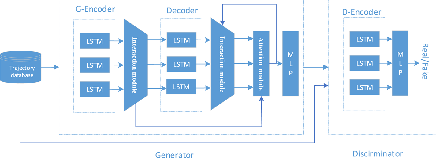
The structure of GAN-AI model is shown in Figure 1. The model consists of a generator and discriminator. The generator consists of a G-encoder, G-decoder, interaction module, attention module and MLP. The discriminator consists of a D-encoder and MLP. During the training, the vessels’ historical trajectory sequence $\textrm{X}$ is encoded by the G-encoder, and the coding matrix of each trajectory ${H_e}$
 is obtained. Through the interaction module, the integrated data C that includes single information and group information is collected. The G-decoder decodes the C as the context information to output the predicted trajectory $\mathrm{\hat{Y}}$
 . The real trajectory and generated trajectory are input into the discriminator to distinguish the reality of the trajectory, and the network parameters of the generator and discriminator are optimised to make the predicted trajectory approach the real trajectory by decreasing the model loss.

Figure 1. Structure of GAN-AI
3.1 Interaction model
An interactive module is used to process and learn the encounter information of multiple ships in the same water area. At time t, the interaction module calculates the difference of coordinates and speeds between the ship i and j to get the relative distance information and relative speed information. Then coding the relative motion information through a fully connected neural network (FCNN) (Sainath et al., Reference Sainath, Vinyals, Senior and Sak2015) to get the hidden interaction information $s_{ij}^t$ , and then stores the group interaction information into a set as ${S^t}$
 . Finally, the individual motion information $H_e^t$
 and the group interaction information ${S^t}$
 are together input into a MLP to obtain integrated state vector. The relevant formulae are:

where ${W_I}$ , ${W_{\tanh }}$
 is the weight matrices of the FCNN and the MLP with tanh activation function that must be trained. $H_e^t$
 is the coding data obtained from the G-encoder and $H_e^t$
 includes the self-motion features of all ships at time t.
3.2 Generator
The generator is mainly composed of a G-encoder and G-decoder, which are used to capture and analyse the semantic information of historical trajectory and generate reasonable future trajectory sequence. In the G-encoder, each trajectory sequence ${\textbf{X}_\textbf{i}}$ is mapped and normalised by an FCNN to obtain vector $E{_i}$
 , and then the $E{_i}$
 is encoded by an LSTM (Bahdanau et al., Reference Bahdanau, Cho and Bengio2014) to obtain the hidden representation of trajectory ${H_{ei}}$
 :
:


where ${W_{em}}$ and ${W_{en}}$
 are the weight matrices of the FCNN and the LSTM that must be trained. ${H_{ei}}$
 is the output of the LSTM neural network, which involves the potential characteristic information of the position, speed, acceleration and so on of vessel i. ${H_{init}}$
 is the initial state of the LSTM's hidden layer which is set by normal distribution. Through N times of processing, we can get the code matrix ${H_e}$
 that includes the self-motion features of N ships in the same water area:

To model the interactive behavior of the multiple ships, we input the ${H_e}$ and the X into the interaction module introduced in Section 3.1. The interaction module can integrate the group motion information and the monomer motion information at time ${t_{obs}}$
 . The output ${C}$
 of interaction module contains the N ships’ own motion information and relative motion information:

To predict the future trajectory point of vessel i at time t, the G-decoder must be input the coordinate data $({x_i^{t - 1},y_i^{t - 1}} )$ and context information $C_i^{t - 1}$
 that were obtained from the last time point, and then the G-decoder can predict the trajectory point coordinates on continuous time points by iteration. At the beginning of prediction, Gaussian noise z is superimposed ${C_i}$
 to get ${C^{\prime}_i}$
 , and the initial hidden state of the LSTM decoder is initialised by ${C^{\prime}_i}$
 to improve the noise reduction ability of the decoder:


where ${W_{ed}}$ , ${W_{de}}$
 is the network matrices of the FCNN and LSTM that must be trained, and $h_{di}^t$
 is the output LSTM. The FCNN in Equation (14) is used to map the coordinate to feature space and the LSTM is used to decode context $C_i^{t - 1}$
 . To solve the problem of memory degradation in the iterative updating process of LSTM and make the model always focus on the real observation data ${C^{\prime}_i}$
 from the G-encoder, ${C^{\prime}_i}$
 and $h_{di}^t$
 are concatenated to calculate the attention weights $a_i^t$
 through the attention module at each update step. The weighted $h_{di}^t$
 can be obtained by multiplying $h_{di}^t$
 and $a_i^t$
 , and then it is employed to achieve coordinate prediction with an MLP. The formula is:


where ${W_d}$ ,${W_{relu}}$
 is the network matrices of the FCNN and MLP that must be trained. The FCNN in Equation (16) is used to calculate the similarity between the $h_{di}^t$
 and ${C^{\prime}_i}$
 to get the attention weights. The MLP is used to shape the vector and output the future position. Finally, the prediction results are input into the interaction module to update the context information $C_i^t$
 , and the $C_i^t$
 can be used to prediction for next time step.
3.3 Discriminator
The discriminator is a classical binary classification model to judge whether the generated trajectory is true or false. The discriminator and the generator compete with each other to make themselves converge at the same time during training. The discriminator maps the trajectory sequences through an FCNN to get feature vector R. An LSTM is used to further encode the R to get ${H_c}$ . Then run ${H_c}$
 through an MLP to output the reality of the trajectories:


where, ${W_{ec}}$ ,${W_c}$
 , ${W_s}$
 are the parameters of the FCNN, LSTM, and MLP that must be trained. ${X_r}$
 is the set of real trajectory sequence, ${X_f}$
 is the set of fake trajectory sequence, ${h_{init}}$
 is the initialisation state parameter of the LSTM network, ${H_c}$
 is the output of the LSTM.
3.4 Loss function
The relative average loss (Wang et al., Reference Wang, Yu, Wu, Gu, Liu, Dong, Qiao and Change Loy2018) is used as the metric to estimate the distribution differences between the fake and the real trajectories. The relative average loss function is defined as the probability that the real trajectory is more realistic than the predicted trajectory in the discriminator. The formulae are:


where ${x_r}$ denotes the real trajectory sequence, ${x_f}$
 denotes the predicted trajectory sequence, and $\sigma$
 is a sigmoid function. In the GAN-AI model, the discriminator is only used to estimate the probability that the input is the real trajectory, so the loss function of the discriminator is defined as:

The generator loss function is composed of $L_G^{Ra}$ and ${L_{L2}}$
 , $L_G^{Ra}$
 is the adversarial loss function of the generator and the discriminator and realises the competition between the discriminator and the generator. ${L_{L2}}$
 is the variety loss (Gupta et al., Reference Gupta, Johnson, Fei-Fei, Savarese and Alahi2018) to encourage GAN-AI to produce diverse samples. It means the generator generates $k$
 trajectories during training and chooses the minimum loss of the real trajectory and the predicted trajectories as the model's loss. The formulae are:


4. Experiment
To assess the correctness and accuracy of the GAN-AI, the historical AIS data of Zhou Shan Port, China, in January 2018 was selected to evaluate the model. That part of the channel is an intersection that is not only narrow but also has high traffic density. A large number of small and medium-sized ships with north-south and east-west directions encounter here every day, causing a complex traffic environment. The experimental data are 2600 ship trajectories, including 2000 trajectories as training data and 600 trajectories as validation data.
4.1 Loss curves of training
To evaluate performance of the GAN-AI, a series of models have been trained and named as ‘GAN-AI-KVN’, where ‘A’ denotes the GAN model assembles the attention module, and ‘I’ denotes the GAN model assembles the interaction Mmodule; ‘K’ means the model uses a variety loss function during the training; ‘N’ refers to the number of sampling time during test time and chooses the best prediction in L2 sense for quantitative evaluation. This paper compares the L2 loss-convergence curves of the classical trajectory prediction model sequence to sequence (Seq2seq), the plain GAN model GAN-10v10, and the improved GAN model: GAN-I-10v10 and GAN-AI-10v10. The initial learning rate is set to 0⋅001, and an Adam (Kingma and Ba, Reference Kingma and Ba2014) optimisation algorithm is used to optimise the network parameters. The batch size is set to 32, and the number of training iterations is set to 1,600. The observation sequence length is set to 9, and the prediction sequence length is set to 9. The sampling interval is 10 s.
The comparison results of the training curve and validation curve of the four models are shown in Figure 2. It can be seen from Figure 2 that the L2 loss of the four models shows a downward trend through iterative training and tends to be stable after 1,600 iterations. Among the four models, GAN-AI-10v10 has the best convergence, and the loss on the validation set is 0⋅331. The second best model is the GAN-I-10v10 model, with a loss of 0⋅358 on the validation set. The loss of the Seq2seq model on the validation data is 0⋅363. The GAN-10v10 model has the worst convergence, only 0⋅398. By observing the convergence trend of the convergence curve, it can be found that although GAN-10v10 finally converges, the convergence curve fluctuates greatly. But GAN-I-10v10 does not appear to have this phenomenon by assembling interactive modules, which can prove that interactive modules can effectively help the GAN network to achieve stable convergence. The GAN-AI-10v10 model achieves better convergence than does the GAN-I-10v10 model by assembling the attention module. It proves that the attention mechanism can help the network capture and grasp the motion information of ships at different times, thus improving the learning ability of the network.

Figure 2. Plots of models’ L2 loss curves: (a) is L2 loss curve of the Seq2seq; (b) is L2 loss curve of the GAN-I-10v10; (c) is L2 loss curve of the GAN-10v10; (d) is L2 loss curve of the GAN-AI-10v10;
4.2 Accuracy and analysis
To evaluate the trajectory prediction accuracy of the GAN-AI model, the average distance error (ADE) and final distance error (FDE) metrics used in reference Gupta et al. (Reference Gupta, Johnson, Fei-Fei, Savarese and Alahi2018) are introduced. ADE calculates the average Euclidean distance between the predicted trajectory and the real trajectory at each time point. The FDE calculates the average Euclidean distance between the predicted trajectory and the real trajectory at the last time point of the prediction period. The formulae are:


This paper has compared the prediction accuracy of six models: seq2seq, GAN-10v10, Kalman model, GAN-I-10v10, GAN-AI-10v10, and GAN-AI-20v20. Among them, seq2seq is the classical nonlinear model, the Kalman model is the classical linear model, and other GAN models are assembled different modules. Table 1 shows the comparison results of the trajectory prediction accuracy of six models on the test data set. It can be found that at the scene of ship encounter, by adding an interaction module, the model can learn ship interaction behaviour, effectively improve the prediction accuracy of the model, and make GAN-I-10v10, GAN-AI-10v10 and GAN-AI-20v20 obtain higher precision than other models without an interaction module. At the same time, by assembling the attention module, the model can improve the ability to extract effective data at multiple time points, so that the ADE of GAN-AI-10v10 is 1⋅8 m/3⋅0 m higher than that of GAN-I-10v10 at different prediction time length. Comparing the model accuracy of GAN-AI-10v10 and GAN-AI-20v20, it can be found that higher sampling times can effectively improve the prediction accuracy of the network during network training and evaluation, making the ADE of GAN-AI-20v20 model reach 28⋅4 m/40⋅7 m. In this paper, the Kalman prediction model gives a benchmark of the linear methods, which is compared with our non-linear method. . Because the linear methods can not model the non-linear motion of vessels and the ADE of the Kalman model only reaches 74⋅2 m/146⋅3 m at different prediction time lengths.
Table 1. Comparison of ADE and FDE of different models

Although ADE and FDE can objectively evaluate the prediction accuracy of the model, it is unable to analyse the reasons for the differences in prediction accuracy of different models. Figure 3 compares the prediction differences of five models in four typical real encounter scenarios. Figure 3a is the prediction result of two ships in the crossing situation, Ship A is an accelerating ship to enter the port after judging the situation, and Ship B keeps straight-line navigation. Comparing the predicted results about Ship B, it can be found that the predicted results of the five models are similarly consistent, and they are consistent with the distribution of the real trajectory in the navigation distance and direction. However, comparing the prediction results about Ship A, Kalman model's ADE/FDE only reaches 197.3m/409.1m that achieved the largest prediction error, as it is a linear model that cannot effectively estimate the turning behavior of the ship. Comparing to the linear method, the other four nonlinear methods can better estimate the navigation trend of the ship's future trajectory. But comparing to the GAN-AI-10v10, the GAN-I-10v10, seq2seq and GAN-10v10 have greater errors in the navigation distance and course. Figure 3b shows the prediction results of two ships in the real overtaking situation. Ship A is a slowly left-turning ship. After judging the situation, Ship B takes the action of overtaking from Ship B's port side. Comparing the prediction results about Ship A, the prediction results of GAN-AI-10v10 are consistent with the real trajectory, and ADE/FDE is 24⋅5 m/25⋅7 m. The GAN-10v10 and GAN-I-10v10 models have errors in the estimation of the navigation speed, but the course estimation is consistent with the real result, while the Seq2seq model is consistent with the real result in the speed, but the course estimation has errors. Comparing the prediction results about Ship B, excepting for the linear method, the other four models are consistent with the real trajectory. Figure 3c is the prediction result in the free situation. Although Ships A and B are in the same water area, they do not have interactive behaviour. For the five prediction results, excepting for the distortion of the linear prediction method, the prediction results of the other four models are similar to the real trajectory temporal–spatial distribution. Figure 3d is the prediction result of the head-on situation. Ship A drives in a straight line after the encounter and turns right at the later part of the journey. Ship B turns left and adjusts to the original route after the encounter. Comparing the prediction results about⋅ Ship A, the prediction results of GAN-AI-10v10 and seq2seq models are better in the former section, but the prediction of the turning track in the latter section has deviation, and the ADE/FDE are 47⋅5 m/95⋅8 m and 49⋅6 m/101⋅4 m. Among the five models, GAN-10v10 is the best, ADE/FDE is 46⋅6 m/33⋅6 m. The results of GAN-I-10v10 were the worst, and ADE/FDE is 77⋅6 m/178⋅4 m. Comparing the results of ship B, the error of GAN-AI-10v10 and GAN-I -10v10 is smaller, and the ADE/FDE are 45⋅8 m/77⋅4 m and 47⋅1 m/81⋅3 m. The results of seq2seq and gan-10v10 are similar to the linear method, and ADE/FDE are greater than 50 m/85 m.

Figure 3. Prediction results of four different situations: (a) is the result in the crossing situation; (b) is the result in the overtaking situation; (c) is the result in the free situation; (d) is the result in the head-on situation
By comparing the trajectory prediction results in four different scenarios, it can be found that the reason for GAN-AI-10v10 attains higher accuracy is that it can better estimate the parameters of course and distance simultaneously in four scenarios. By assembling the interactive module, the GAN-AI-10v10 model can better learn the ship's course and speed changes. By assembling the attention module, the GAN-AI-10v10 model can better allocate the parameter weight of the model and improve the spatiotemporal modelling ability of the model. On the other hand, the GAN-I-10v10 model has a wrong estimation of speed in the case of Figures 3a and 3b due to the lack of attention mechanism. The seq2seq and GAN-10v10 models have error estimation of course in Figures 3a and 3b due to the lack of interaction modules. It indicates that the attention module and interaction module can improve the accuracy of speed and course estimation.
4.3 Analysis of variety loss
A series of models of GAN-AI-NVN have been trained to evaluate the influence between the performance and the variety loss function. ‘NvN’ indicates the GAN-AI using the variety loss fuction during the training. ‘N’ refers to the number of times we sample from GAN-AI model during test time. As shown in Figure 4 the model can get better performance with the increase of N and the performance gets about 30% better with N = 70. On the other hand, the model's computation will be increasing accordingly with N and the rise of accuracy will be slower. As a result, N = 20 is a pretty setting for computation and accuracy.

Figure 4. Effect of variety loss
5. Conclusion
A GAN-AI model is proposed to predict the trajectory of multiple ships in the same water area simultaneously. In the GAN-AI model, an attention module is designed to improve the ability of the network to extract effective data and avoid memory degradation of LSTM. An interaction module is designed to model the interaction behaviour information, such as relative distance and relative speed between ships, so as to get better performance in complex interactive scenes. To improve the convergence ability and prediction accuracy of the network, the adversarial loss function and variety loss function are introduced into the network training. Using the ADE and FDE metrics to verify the GAN-AI model on the real AIS historical data, the results show that the ADE/FDE of the GAN-AI-20V20 model is less than 40⋅7 m/82⋅4 m under the prediction duration of 180s. Compared with seq2seq, plain GAN and Kalman models, the performance has been improved by 20%, 24% and 72%, respectively. It is of great significance to improve the strength of the vessel traffic management system, the path planning of intelligent ships and the analysis of ship collision risk. On the other hand, more AIS data should be extracted to validate the model's generalisation ability and data fusion can also be utilised to improve the accuracy further in future work.
Funding statement
The research reported here was sponsored by Sanya Science and Education Innovation Park of Wuhan University of Technology (Grant No. 2020KF0040), the Key Research Plan of Zhejiang Provincial Department of Science and Technology (Grant No. 2021C01010).
Competing interests
The authors declare no conflicts of interest.